| Issue |
A&A
Volume 706, February 2026
|
|
|---|---|---|
| Article Number | A165 | |
| Number of page(s) | 18 | |
| Section | Extragalactic astronomy | |
| DOI | https://doi.org/10.1051/0004-6361/202556597 | |
| Published online | 06 February 2026 | |
Rapid, out-of-equilibrium metal enrichment indicated by a flat mass-metallicity relation at z ∼ 6 from NIRCam grism spectroscopy
1
Institute of Science and Technology Austria Am Campus 1 3400 Klosterneuburg, Austria
2
National Astronomical Observatory of Japan 2-21-1 Osawa Mitaka Tokyo 181-8588, Japan
3
Astronomy Centre, University of Sussex, Falmer Brighton BN1 9QH, UK
4
Department of Physics, North Carolina State University Raleigh 27695 North Carolina, USA
5
Institute for Computational & Data Sciences, The Pennsylvania State University University Park PA 16802, USA
6
Institute for Gravitation and the Cosmos, The Pennsylvania State University University Park PA 16802, USA
7
Kavli Institute for Cosmology, University of Cambridge Madingley Road Cambridge CB3 0HA, UK
8
Cavendish Laboratory, University of Cambridge JJ Thomson Avenue Cambridge CB3 0HE, UK
9
Department of Astronomy, University of Wisconsin-Madison 475 N. Charter St. Madison WI 53706, USA
10
Centro de Astrobiología (CAB), CSIC-INTA Carretera de Ajalvir km 4 Torrejón de Ardoz E-28850 Madrid, Spain
11
Cosmic Dawn Center (DAWN), Denmark
12
Niels Bohr Institute, University of Copenhagen Jagtvej 128 2200 Copenhagen N, Denmark
13
Department of Astronomy, University of Geneva Chemin Pegasi 51 1290 Versoix, Switzerland
14
Laboratory of Astrophysics, École Polytechnique Fédérale de Lausanne (EPFL), Observatoire de Sauverny 1290 Versoix, Switzerland
15
MIT Kavli Institute for Astrophysics and Space Research, Massachusetts Institute of Technology Cambridge MA 02139, USA
16
BNP Paribas Corporate & Institutional Banking Torre Ocidente Rua Galileu Galilei 1500-392 Lisbon, Portugal
★ Corresponding author: This email address is being protected from spambots. You need JavaScript enabled to view it.
Received:
25
July
2025
Accepted:
25
November
2025
Abstract
We aim to characterise the mass-metallicity relation (MZR) and the 3D correlation between the stellar mass, metallicity, and star formation rate (SFR) known as the fundamental metallicity relation (FMR) for galaxies at 5 < z < 7. Using ∼800 [O III] selected galaxies from deep NIRCam grism surveys, we present our stacked measurements of direct-Te metallicities, which we used to test recent strong-line metallicity calibrations. Our measured direct-Te metallicities (0.1–0.2 Z⊙ for M★ ≈ 5 × 10⁷ − 9 M⊙, respectively) match recent JWST/NIRSpec-based results. However, there are significant inconsistencies between observations and hydrodynamical simulations. We observe a flatter MZR slope than the SPHINX20 and FLARES simulations, which cannot be attributed to selection effects. With simple models, we show that the effect of an [O III] flux-limited sample on the observed shape of the MZR is strongly dependent on the FMR. If the FMR is similar to the one in the local Universe, the intrinsic high-redshift MZR should be even flatter than is observed. In turn, a 3D relation where SFR correlates positively with metallicity at fixed mass would imply an intrinsically steeper MZR. Our measurements indicate that metallicity variations at fixed mass show little dependence on the SFR, suggesting a flat intrinsic MZR. This could indicate that the low-mass galaxies at these redshifts are out of equilibrium and that metal enrichment occurs rapidly in low-mass galaxies. However, being limited by our stacking analysis, we are yet to probe the scatter in the MZR and its dependence on SFR. Large carefully selected samples of galaxies with robust metallicity measurements can put tight constraints on the high-redshift FMR and help us to understand the interplay between gas flows, star formation, and feedback in early galaxies.
Key words: galaxies: abundances / galaxies: evolution / galaxies: formation / galaxies: high-redshift / galaxies: ISM
© The Authors 2026
 Open Access article, published by EDP Sciences, under the terms of the Creative Commons Attribution License (https://creativecommons.org/licenses/by/4.0), which permits unrestricted use, distribution, and reproduction in any medium, provided the original work is properly cited.
This article is published in open access under the Subscribe to Open model. This email address is being protected from spambots. You need JavaScript enabled to view it. to support open access publication.
1. Introduction
The gas-phase metallicity of the interstellar medium of galaxies reflects the interplay of gas inflows, feedback, and star formation (Finlator & Davé 2008; Lilly et al. 2013; Maiolino & Mannucci 2019; Curti 2025). Usually, the gas-phase metallicity is expressed in terms of the oxygen abundance (relative to the hydrogen abundance) as it is the most abundant metal in the Universe. It is most easily observed through strong lines in star-forming regions of galaxies, such as [O II]λλ3726, 3729 and [O III]λλ4960, 5008. Studying the evolution of the gas-phase metallicities of galaxies through cosmic time can tell us about the baryonic mass assembly in the Universe.
The relation between gas-phase metallicity (Zgas) and stellar mass (M★), known as the mass-metallicity relation (MZR), has been extensively studied, spanning from galaxies in the local Universe (at z ∼ 0, e.g. Tremonti et al. 2004; Ellison et al. 2008; Moustakas et al. 2011; Andrews & Martini 2013; Curti et al. 2020; Scholte et al. 2024), to those at the peak of cosmic star formation activity (up to z ∼ 3; e.g. Shapley et al. 2005; Maiolino et al. 2008; Mannucci et al. 2009; Wuyts et al. 2014; Topping et al. 2021; Sanders et al. 2021), and well into the epoch of reionisation using JWST (e.g. Heintz et al. 2023; Matthee et al. 2023; Nakajima et al. 2023; Chemerynska et al. 2024; Laseter et al. 2024; Curti et al. 2024; Sanders et al. 2024; Sarkar et al. 2025; Chakraborty et al. 2025; Morishita et al. 2024; Cullen et al. 2025; Li et al. 2025; Pollock et al. 2025). It has been observed that the gas-phase metallicity of galaxies increases with increasing stellar mass, and for z < 4 the slope of this trend becomes shallower at higher masses. This trend is explained through gas regulation in galaxies (Finlator & Davé 2008; Peeples & Shankar 2011; Davé et al. 2012; Lilly et al. 2013). Due to higher stellar masses, the galaxies have a deeper potential well, making the outflow of metal-enriched gas from the galaxy difficult. The metallicity also decreases at fixed stellar mass with increasing redshift. The redshift evolution of the MZR could be due to the inflow of metal-poor gas, or the outflow of metal-rich gas due to stronger feedback mechanisms at higher redshifts (Lara-López et al. 2010; Bothwell et al. 2013, 2016; Scholte et al. 2024). This evolution has also been studied in terms of the 3D relation between the gas-phase metallicity, stellar mass, and star formation rate (Mannucci et al. 2010; Lara-López et al. 2010; Andrews & Martini 2013; Curti et al. 2020, SFR). The scatter in the MZR in the local Universe can be reduced by accounting for variations in the SFRs of galaxies. Galaxies in the local Universe are found to reside on a 2D plane in the M★-Zgas-SFR space with < 0.1 dex scatter. This relation is known as the fundamental metallicity relation (FMR). Multiple studies have found that the FMR remains invariant up to z ∼ 3 (Cresci et al. 2012; Maier et al. 2015; Yabe et al. 2015; Topping et al. 2021; Sanders et al. 2021). Nakajima et al. (2023) and Sarkar et al. (2025) find no redshift evolution for their sample between 4 < z < 8 compared to the z = 0 FMR, but observe significant deviations at z > 8. Various theoretical models and simulations also explore the FMR in terms of the SFR on different spatial (Wang & Lilly 2021) and temporal scales (Torrey et al. 2018; Ma et al. 2024), the impact of different feedback mechanisms (De Rossi et al. 2017), and variations in gas flows and the gas fraction (Dayal et al. 2013; Torrey et al. 2019).
There are several arguments about whether the FMR exists out to high redshifts (e.g. Zahid et al. 2014; Heintz et al. 2023; Curti et al. 2024; Scholte et al. 2025; Cullen et al. 2025). If truly fundamental, the shape of the FMR plane does not evolve – only the relative position of the galaxy population on the plane shifts. Simulations suggest that the existence of the plane depends on the timescales of SFR variability (e.g. Torrey et al. 2018; Ma et al. 2024). Given that the star formation histories (SFHs) of high-z galaxies appear more bursty (e.g. Topping et al. 2022; Endsley et al. 2023; Looser et al. 2025), it could cause the FMR to break down at high-z. Indeed, some JWST studies indicate that the normalisation of the plane shifts, i.e. galaxies systematically have lower metallicities than is predicted by the z = 0 FMR (Heintz et al. 2023; Curti et al. 2024; Scholte et al. 2025).
Gas-phase metallicity is typically inferred using two approaches: (1) the direct-Te method, and (2) strong-line calibrations. The direct-Te method is based on electron temperature (Te) determination using auroral emission lines. The most common auroral line used to determine the electron temperature of the O+2 regions is [O III]λ4364 (Maiolino & Mannucci 2019; Curti 2025). The relative strength of the [O III]λ4364 and [O III]λ5008 lines can be used to calculate the electron temperature. The calculated electron temperature is then used to estimate the gas-phase metallicity using dust-corrected emission line ratios of [O III] and [O II] with Hβ. The challenge with this method is that the [O III]λ4364 auroral line is very faint, and thus hard to detect in most galaxies (Osterbrock & Ferland 2006; Kewley et al. 2019).
On the other hand, the strong line method is applicable to a larger dataset as it only requires the detection of emission lines that are easily observable in the star-forming regions of the galaxies. The strong line metallicity calibrations are usually calibrated to metallicity measurements from the direct-Te method. Multiple studies have constructed metallicity calibration curves using the observed relationship between emission line ratios and the direct-Te method metallicity estimates for galaxies (e.g. Maiolino et al. 2008; Marino et al. 2013; Andrews & Martini 2013; Bian et al. 2018; Curti et al. 2020; Nakajima et al. 2022; Laseter et al. 2024; Chakraborty et al. 2025; Sanders et al. 2024; Scholte et al. 2025). Some of the calibration curves were developed using galaxies that are considered to be high-redshift analogues (Bian et al. 2018; Nakajima et al. 2022). These calibrations offer a potential solution to estimate metallicity at high-z where getting direct-Te metallicities is difficult; however, their applicability at these redshifts needs to be tested.
Recent studies using JWST make use of strong-line calibrations to explore the MZR at a redshift range of z = 3–10 (Matthee et al. 2023; Nakajima et al. 2023; Li et al. 2023; Heintz et al. 2023; Curti et al. 2024; Sarkar et al. 2025; Chemerynska et al. 2024; Rowland et al. 2025; Li et al. 2025; Cataldi et al. 2025; Pollock et al. 2025). Studies by Nakajima et al. (2023), Sanders et al. (2024), Laseter et al. (2024), Sarkar et al. (2025), Chakraborty et al. (2025), and Pollock et al. (2025) use the [O III]λ4364 auroral line (direct-Te method) to investigate the MZR up to z ∼ 10. Most of these studies mainly focus on galaxies with log(M★/M⊙) > 8. Analysis by Curti et al. (2024) and Chemerynska et al. (2024) explores the MZR down to log(M★/M⊙)∼6 at high redshifts. Considering JWST’s recent arrival on the scene, the sample sizes for which we have direct-Te measurements are still limited.
In this work, we study and characterise the MZR and the 3D correlation with SFR between 5 < z < 7 through direct-Te metallicities using data from deep NIRCam grism surveys EIGER (Kashino et al. 2023), COLA1 (Torralba-Torregrosa et al. 2024) and ALT (Naidu et al. 2024). Our sample makes use of NIRCam spectra, compared to most of the studies in the literature, which use JWST/NIRSpec. Grism spectra have a simple flux-limited selection function and are not subject to slit losses. On the other hand, they are less sensitive and have a smaller wavelength coverage than NIRSpec spectra. Our galaxy sample was selected by using only the [O III]λλ4960, 5008 flux in all three surveys, giving us a well defined, flux-limited selection function. We cover the Hβ and [O III]λλ4960, 5008 emission lines for all our galaxies and, for a subset, we also cover Hγ and [O III]λ4364. For this subset we measured the [O III]λ4364 auroral line with a signal-to-noise ratio (S/N) of > 3 in stacks of stellar mass bins, which we used to calculate the direct-Te metallicities. We used these measurements to test the strong-line calibrations high-z galaxies, obtain a scaling relation between the gas-phase metallicity and stellar mass, and investigate the impact of our selection function.
The paper is structured as follows. We describe our NIRCam grism dataset and data reduction pipeline in Sect. 2. We report the method of extracting emission line fluxes and dust correction in Sect. 3. In Sect. 4 we describe deriving metallicities using both the direct-Te method and strong-line calibrations, and in Sect. 5 we present our MZR and make comparisons to the literature. Furthermore, we discuss the impact of our selection function in Sect. 6 through comparisons to simulations and toy models. Finally, we present our conclusions and summary in Sect. 7.
Throughout this work, we adopt a flat ΛCDM cosmology with ΩΛ = 0.69, ΩM = 0.31, and H0 = 67.7 km s−1 Mpc−1 (Planck Collaboration VI 2020). All magnitudes are mentioned in the AB system (Oke & Gunn 1983).
2. Data
2.1. Observations
We used a compilation of imaging and Wide Field Slitless Spectroscopy (WFSS) from deep NIRCam grism surveys. The data were obtained from the EIGER survey (programme ID 1243, PI Lilly, Kashino et al. 2023), the ALT survey (programme ID 3516, PIs Matthee and Naidu, Naidu et al. 2024), and the JWST programme ID 1933 (PIs Matthee and Naidu, hereafter ‘COLA1 survey’). The EIGER survey is a deep grism cycle 1 survey in the F356W filter centred on six widely separated z > 6 quasar fields. It contains imaging in the short-wavelength (SW) filters F115W and F200W, and direct imaging in the F356W long-wavelength (LW) filter. Each field has a survey area of 6.5 × 3.4 arcmin2 (i.e. 132 arcmin2 in total).
The WFSS in the F356W LW filter covers an observed wavelength of 3.1–4.0 μm with a spectral resolution of R ∼ 1600 for a point source. The COLA1 survey has a similar observing strategy to EIGER, but is centred on the bright double-peaked Lyα emitter, COLA1, at z = 6.6 (Matthee et al. 2018; Torralba-Torregrosa et al. 2024). The total area in the COLA1 field is 21 arcmin2. Finally, the ALT survey is the deepest NIRCam WFSS survey to date, targeting a wider 30 arcmin2 area around the gravitational lensing cluster Abell 2744 in the F356W filter. Thanks to deep imaging from UNCOVER (programme ID 2561, PI Labbe, Bezanson et al. 2024) and MegaScience (programme ID 4111, PI Suess, Suess et al. 2024), there is excellent photometric coverage, allowing for a detailed characterisation of the SEDs for galaxies from the ALT survey. From ALT, we only selected galaxies with magnification factor (μ) < 3 to remove multi-imaged sources and strong arcs.
2.2. Data reduction
In this work, we focus on [O III]λλ4960, 5008 selected galaxies that are observed in the NIRCam WFSS with the F356W filter (λ ∼ 3.1–4.0 μm) in the redshift range 5.5 < z < 7. The analysis in our paper makes use of both JWST/NIRCam imaging and WFSS. The details of the basic reduction steps are described in Kashino et al. (2023, 2025) for the EIGER survey, Torralba-Torregrosa et al. (2024) for the COLA1 survey, and Naidu et al. (2024) for the ALT survey. Here we briefly summarise the WFSS data reduction steps for these surveys and additional modifications made for emission-line spectra extraction.
The WFSS data were reduced using a combination of the JWST pipeline and customised Python-based processing. We downloaded the RATE files from the MAST database1 and used the JWST pipeline to flat field images. For the images in the COLA1 and EIGER fields, we subtracted the background by calculating the median value along each column (which is orthogonal to the dispersion direction). For the ALT data in the Abell 2744 cluster, the median statistic was boosted by diffuse light from the vast number of sources (in particular cluster galaxies). We therefore constructed (for each module) a master-background template based on the backgrounds in the COLA1 and EIGER data and scaled the mode of each ALT grism image to the mode value of the background template. We aligned the astrometry of each image by matching the WCS of the image taken simultaneously in the SW filter to the reference catalogue based on the direct imaging in the F356W filter. In our basic reduction used to identify the sources, we separated the dispersed light in a ‘continuum’ and an ‘emission-line’ image, by estimating the continuum in each row with a running median filter along the dispersion direction. The filter is a kernel with width 51 pixels and a central hole of 9 pixels, to avoid over-subtraction of emission-lines. As is detailed in Kashino et al. (2023), this procedure was run twice, masking identified emission-lines from the first iteration.
In this study, we present an improved method for the extraction of emission-line (EMLINE) spectra to avoid over-subtraction around emission lines. This was performed already in Matthee et al. (2024), but here we generalise it for [O III] emitters. The standard methodology can lead to slight over-subtraction of faint wings that are not identified in individual images. Building upon the aforementioned works for the EIGER, COLA1, and ALT surveys, we know the location of the emission lines in our spectra, which allows us to subtract the continuum optimally without over-subtracting line emission. We used this information and stacked the EMLINE spectra of galaxies with a [O III]λ5008 signal-to-noise ratio (S/N) > 25. The methodology for stacking is described further in Sect. 3.3. Once we had the stacked EMLINE spectra, we generated 2D Gaussian masks, with a full width at half maximum of 7 pixels and size of 15 pixels with a threshold of 1 × 10⁻²⁰ erg s−1 cm2, for the [O III]λλ4960, 5008 emission lines using the Photutils Python package (Bradley et al. 2024). The mask for the [O III]λ5008 line was applied to its respective location, while the mask for the [O III]λ4960 line was applied to the locations of [O III]λ4960, Hγ, [O III]λ4364, and Hβ in each 2D science (SCI) spectrum in our sample. We applied the mask for [O III]λ4960 to the other emission lines (Hγ, [O III]λ4364, and Hβ) due to their smaller flux compared to [O III]λ5008. Utilising the [O III]λ5008 mask for these lines could result in over-masking, which can cause under-subtraction of the continuum and can cause the potential overlap with adjacent emission lines, especially for the Hγ and [O III]λ4364 emission lines. After applying the masks to the SCI spectra, we performed the continuum subtraction on the SCI spectra using a running box-car median with a kernel of 71 pixels and a gap of 7 pixels in the centre, similar to the method in the initial extraction of emission-line spectra. The parameters were iteratively chosen based on stacked spectra, whereby we optimised to match the line shapes and the 1:2.98 normalisation of the [O III]λλ4960, 5008 doublet.
3. Methods
3.1. Galaxy sample
Our dataset comprises [O III]λλ4960, 5008 selected galaxies from the EIGER (Kashino et al. 2025), COLA1 (Torralba-Torregrosa et al. 2024), and ALT (Naidu et al. 2024) surveys. These galaxies were selected using the ‘forward’ method described in Kashino et al. (2023). In this method, the [O III] doublet sample are required to have S/N > 3 and a maximum offset of 3 pixels (0.09″) in their spatial centroid. Once we had our emission line spectra, the galaxies were inspected to detect any broad line Hβ emission. We did this to find possible broad-line active galactic nucleus (AGN) candidates and remove them from our sample. We excluded the spectra for the central quasars in the EIGER fields. We also removed AGNs that are known from previous studies, such as the X-ray detected AGN J1148+5253 (Mahabal et al. 2005) at z = 5.69. We also removed the galaxy J0100−9148 from our sample because of severe contamination in the 2D spectra. We did not find additional broad Hβ emitters in our sample; however, it should be noted that broad-line Hα AGNs at high redshifts usually have extremely faint broad Hβ emission (Brooks et al. 2025). Through this, we obtained a dataset of 792 galaxies, of which 659 galaxies are from the EIGER survey, 74 are from the COLA1 survey, and 59 are from the ALT survey. We classified our data into two samples:
-
(i)
-
The Hβ sample: galaxies for which our data cover the Hβ emission line at a rest-frame wavelength of 4862.68 Å, i.e. galaxies with a redshift of 5.5 ≤ z < 7. This is the entire dataset with 792 galaxies.
-
(ii)
The Hγ sample: galaxies for which our data cover the Hγ emission line at a rest-frame wavelength of 4340 Å, i.e. galaxies with a redshift of 6.3 ≤ z < 7. This is a subset of the Hβ sample, with 270 galaxies.
The typical UV magnitudes of the Hγ and the Hβ sample are MUV = −19.5 mag and −19.4 mag, respectively (see Fig. 1). Stellar masses in our total dataset range from log(M★/M⊙) = 6.9–11.1, with typical stellar masses of both samples being ∼108.3 M⊙. Our sample is stellar mass complete down to log(M★/M⊙)∼8.5 (see Fig. 1). Properties such as stellar mass, emission line fluxes, and photometry for the galaxies from the ALT catalogue were corrected for magnification using magnification factors from Furtak et al. (2023) and Price et al. (2025). The redshift uncertainty for our sample is ∼60–70 km s−1 (Torralba-Torregrosa et al. 2024; Naidu et al. 2024; Kashino et al. 2025).
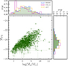 |
Fig. 1. Relation between UV magnitude and stellar mass for our Hβ sample (792 galaxies). The MUV and stellar masses were obtained through SED fitting using Prospector. With data from the ABELL2744 lensing field, we probed galaxies with MUV down to −16.6 mag. The UV luminosity increases with stellar mass, as was expected. |
3.2. SED modelling
In order to estimate galaxy properties such as the stellar mass, we performed SED fitting using the code Prospector (Johnson et al. 2021). Nebular emission was self-consistently modelled based on the photoionisation code Cloudy (Ferland et al. 1998, 2013). The stellar population modelling was implemented through FSPS (Conroy et al. 2009; Conroy & Gunn 2010) using the MIST stellar models (Dotter 2016; Choi et al. 2016). We used a non-parametric SFH with seven bins, adopting a ‘bursty continuity’ prior. The first two bins were fixed at look-back times of 0–5 Myr and 5–10 Myr with the rest logarithmically spaced out to z = 20. We adopted a Chabrier (2003) initial mass function (IMF), with a cut-off at 150 M⊙. The other free parameters are the total stellar mass formed, stellar metallicity, gas-phase metallicity, dust attenuation (a screen and an additional component for young stars), and ionisation parameter. The set-up for the SED fitting is described in detail in Naidu et al. (2022, 2024), which is a modification of the prescription by Tacchella et al. (2022). It should be noted that the derived stellar masses are strongly dependent on the assumed SFH model. Whitler et al. (2023) find that non-parametric models with continuity prior can infer stellar masses up to an order of magnitude larger (an order of magnitude smaller sSFR) than the constant SFH models at the ages of ≲10 Myr.
The SED modelling was done using photometric data and emission-line fluxes from the spectra. The photometric data used for SED fitting of galaxies from the EIGER, COLA1, and ALT survey varies due to differences in photometric filter coverage. For galaxies from the EIGER survey, we used photometry in the F115W, F200W, and F356W filters. In the COLA1 survey, we have photometry in an additional band, F150W, which we included in the SED modelling. For galaxies from the ALT survey, we have photometry from numerous programmes that targeted the Abell 2744 field (primarily UNCOVER; Bezanson et al. 2024 and MegaScience; Suess et al. 2024) totalling 27 filters available for the SED fitting2. For the galaxies from the EIGER and COLA1 surveys, we additionally used the Hβ and the [O III]λλ4960, 5008 emission line fluxes derived from the grism spectra. For the ALT galaxies, the emission line fluxes are de facto included due to the photometry in the various medium-band filters. We verified that there are no systematic biases between the stellar masses from the EIGER/COLA1 surveys versus the ALT survey by confirming that the relation between observed (magnification-corrected) F200W magnitude with the stellar mass is similar across the fields. We also confirmed that in the ALT data the emission-line fluxes from grism data are consistent with those inferred from medium-band photometry (Mascia et al. in prep).
3.3. Stacking grism spectra
Emission lines in the spectrum of a galaxy are a probe of the physical conditions of the ISM. However obtaining a high S/N for faint emission lines such as Hγ or [O III]λ4364 in individual galaxies is difficult with NIRCam grism data. In such cases, stacking methods can extract average measurements by reducing random noise fluctuations at the expense of losing information on individual sources, and therefore variation across the stacked sample. For illustrative purposes, we show the 1D stacked spectra of all the galaxies in our dataset in Fig. 2. The 2D spectra have been brought to rest-frame and normalised by their ([O III]λ5008+2.98[O III]λ4960)/2 luminosity before stacking. From the 2D stacked spectrum, we extracted the 1D spectrum as described in Sect. 3.4.1. We can see strong [O III]λλ4960, 5008 and Hβ emission lines along with the Hγ, Hδ, and [O III]λ4364. We also see the HeI-5877 emission line in the stacked spectrum, although it is relatively faint. In comparison to the stacks presented in Roberts-Borsani et al. (2024) for galaxies between z = 5–7, we detect almost all the key emission lines over the same wavelength range (4000–6000 Å). Additionally, we resolve the [O III]λλ4960, 5008 doublet, and Hγ and [O III]λ4364 due to the higher resolution of NIRCam/WFSS spectra in the F356W filter (R∼1600). Although our grism spectra have a higher resolution, our wavelength coverage is limited compared to the NIRSpec/Prism spectrum, which covers from 1000 to 7000 Å in the same redshift range.
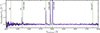 |
Fig. 2. Median stacked 1D rest-frame emission-line spectrum of the full sample of 792 [O III] emitters at z = 5.5–7. Each galaxy spectrum has been normalised by its ([O III]λ5008+2.98[O III]λ4960)/2 flux before stacking. The shaded green region shows the uncertainty estimated through bootstrap resampling. We highlight the wavelengths of Hδ, Hγ, [O III]λ4364, Hβ, [O III]λλ4960, 5008, and HeIλ5877. For visualisation, we normalised the stacked spectrum by the Hβ luminosity such that Hβ peaks at unity. |
After dividing our data into Hγ (6.3 ≤ z < 6.9) and Hβ (5.5 ≤ z < 6.9) samples and obtaining our emission-line spectra, as is described in Sect. 2, we performed median stacking of the emission-line spectra in stellar mass bins. In order to stack the spectra, we shifted the 2D spectrum of each galaxy to the rest-frame wavelength grid ranging from 4000 to 6000 Å through linear interpolation resampling. We verified that our resampling is flux-conserving. We then normalised the 2D spectrum of each galaxy by its respective ([O III]λ5008+2.98[O III]λ4960)/2 luminosity. This allowed us to ensure that the stacks represent the typical line ratios of the spectra and are not dominated by more luminous galaxies. We obtained the stacked spectra by calculating the median over the 300 bootstrap (with replacement) realisations. The uncertainties were obtained by calculating the standard deviation of these bootstraps. The median-stacked spectra of our Hγ sample is shown in Fig. 3.
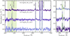 |
Fig. 3. Median stacked 1D rest-frame emission-line spectra of the Hγ sample (z = 6.3–7), in three stellar mass bins offset for visualisation purposes. The shaded region shows the uncertainty estimated through bootstrap resampling. In the right panel, we zoom into the wavelength range containing Hγ and [O III]λ4364. We fitted a complex of three Gaussians with the same standard deviation to obtain the fluxes of Hγ and [O III]λ4364. An additional Gaussian component was fitted to account for possible contamination by [Fe II]λ4360. |
Metallicity and SFR measurements in bins of stellar mass for the Hγ sample with 6.3 < z < 7.
3.4. Measuring emission-line luminosity
3.4.1. Extracting 1D spectra
We measured line luminosities based on optimally extracted 1D spectra (Horne 1986; Matthee et al. 2023). We collapsed the [O III]λ5008 emission line over a wavelength range of ±400 km/s with respect to its wavelength (5008.24 Å). We then performed non-linear least squares fitting of the spatial profile using the lmfit Python package, finding that a Gaussian profile suffices. Subsequently, we collapsed the 2D spectra by assuming the same spatial profile at all wavelengths. The uncertainty on the 1D spectrum was obtained by propagating the uncertainties of the 2D spectrum that we estimated from bootstrapping.
3.4.2. Emission line luminosity measurements
We obtained measurements of the luminosities for [O III]λ5008, [O III]λ4960, Hβ, Hγ, and [O III]λ4364 from our 1D continuum-subtracted stacks using the lmfit Python package. We followed a similar methodology to the one presented in Matthee et al. (2023). We had the best S/N for the [O III]λλ4960, 5008 emission lines, which might have aided us in detecting the natural broadening of the emission lines that give it non-Gaussian wings (Lorentzian wings). However, in our case the extended shapes in the wings of the lines are most likely due to the spatial-spectral degeneracy inherent to grism data (i.e. the spatial extent of the galaxies in the dispersion direction broadens the lines in the grism spectra). Therefore, for [O III]λ5008 and [O III]λ4960 we used a Voigt profile. We fixed the standard deviation (σ) and the Gamma parameter to be the same for the [O III] doublet. We also fixed the emission-line ratio between the doublet to be 2.983. We fitted a similar Voigt profile to the Hβ line so that we traced the emission lines coming from the same gas. We fixed the standard deviation, the Gamma parameter, and the amplitude ratio between the Gaussian and Lorentzian profiles to match the [O IIIλ5008] line. The other emission lines are much fainter; therefore, a Gaussian profile is used, as a Voigt profile does not improve the reduced χ2 of the fits, nor is there significant flux in the wings. The errors on the emission-line luminosities were propagated from the standard error and the covariance matrix obtained from lmfit.
3.5. Dust correction
The luminosities of emission lines can be affected by dust attenuation; thus, it is important to account for it to accurately estimate the gas-phase metallicity for galaxies. Dust attenuation correction for emission line ratios such as [O III]λ5008/Hβ should be negligible, though, as the emission lines are close in wavelength. We calculated the intrinsic, dust-corrected luminosity for [O III]λ5008, [O III]λ4364, and Hβ assuming the Cardelli et al. (1989) nebular attenuation curve in our Hγ sample stack,
 (1)
(1)
where
 (2)
(2)
and
kλ is the attenuation curve, which is wavelength-dependent, and 0.473 is the intrinsic Hγ/Hβ line flux ratio that is appropriate for Case B recombination at 104 K (Osterbrock & Ferland 2006). We measured typical Hγ/Hβ values of 0.37 ± 0.04 at average [O III] temperatures of ∼16 600 K. This indicates some level of dust attenuation; however, we find that the average dust-corrected [O III]λ5008/Hβ (R3) and [O III]λ5008/[O III]λ4364 ratios are only 0.01 dex and 0.03 dex lower than the average dust-uncorrected ratios, respectively.
The [O III]λ5008/Hβ ratios for the Hβ sample stacks are not dust-corrected as we do not always cover the Hγ line required to calculate Balmer decrements and the lines are close in wavelength range. In Fig. 4, we show the [O III]λ5008/Hβ ratios obtained for our stacked samples, along with ratios for individual galaxies in our entire dataset. For our stacks, we consider all Hβ observations as focusing only on S/N(Hβ) ≥ 3 detections would bias our stacked values to lower ratio values at the low-mass end. Applying a selection cut based on S/N(Hβ) would impose additional biases in our sample that would impact our analysis of the MZR. The [O III]λ5008/Hβ ratio seems relatively invariant with stellar mass for the stacked samples. Additionally, the average ratios for both Hγ and Hβ sample stacks are within 0.0009 dex of each other, which suggests that results obtained for the Hγ sample can be applied to the Hβ sample (see Fig. 4).
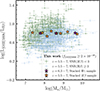 |
Fig. 4. R3 ratio as a function of stellar mass ratios for the entire dataset. Galaxies with S/N(Hβ) ≥ 3 are shown in blue and galaxies with S/N(Hβ) < 3 are shown in green with lower limits. Stars show measurements in stacked spectra. |
4. Metallicity measurements
4.1. Direct method metallicity measurements
We followed the prescription described in Izotov et al. (2006) to estimate the gas phase metallicity using the direct-Te method. For our Hγ sample, we detected the faint auroral line [O III]λ4364 with S/N > 3 in the stellar mass binned stacks. As the [O III]λ4364/[O III]λ5008 ratio is highly temperature-dependent, we can use these detections to derive the electron temperature and the metallicities directly. We do not detect any [O II] emission lines that are required to calculate the electron density and the ionisation state of the gas as they are out of our observable spectral range. Therefore, we assumed an electron density (ne) of 300 cm−3 as has been reported for similar low-metallicity, high-redshift galaxies in the literature (Sanders et al. 2016; Curti et al. 2024; Isobe et al. 2023; Matthee et al. 2023; Sanders et al. 2024; Topping et al. 2025). Recent work by Scholte et al. (2025) and Pollock et al. (2025), probing the ISM for galaxies between z ∼ 5.5–10, suggests that Te measurements and derived abundances are relatively insensitive to the electron density values, ne ≲ 104 cm−3. We find that for an electron density between 100 ≤ ne(cm−3) ≤ 104, our calculated abundances change by 0.02 dex at most. We also assume the O32 ratio – log([O IIIλ5008]/[O II]λλ2727, 29) – to follow a Gaussian distribution with a mean of 0.98 and standard deviation of 0.36, as has been observed by Cameron et al. (2023) for galaxies in the JADES survey between 5.5 < z < 9.5. We find that their sample probes a similar dynamic range in MUV and [O III]λ5008/Hβ ratio as our entire sample. We find that the average [O III]λ5008/Hβ ratio for our Hγ sample lies 0.06 dex above the average value for z ∼ 6 galaxies in Cameron et al. (2023). This can imply that the O32 ratios may be higher than assumed, which would lead to lower metallicities. To confirm this, we would require individual measurements covering both the [O III] and [O II] doublets. We used the Te[O III]-Te[O II] relation given for low gas-phase metallicity from Izotov et al. (2006). With the dust-corrected [O III]λ5008/[O III]λ4364 and the assumed O32 ratio and ne values, we estimated the O2+ and O+ gas temperature using the Python package PyNeb (Luridiana et al. 2013).
We calculated the total oxygen abundance assuming that there is only O+ and O2+ present in the HII region. As we did not detect He IIλ4686, a high ionisation energy line, in our stacked spectra, we did not add O3+ ion abundance to our oxygen abundance (Izotov et al. 2006) as O3+ requires an even higher ionisation potential energy to be excited:
 (3)
(3)
The temperature of O2+ gas ranges from 1.3 × 10⁴ K to 2.1 × 10⁴ K in our stacked sample, and the temperature of O+ gas ranges from 1.3 × 10⁴ K to 1.6 × 10⁴ K. The metallicities of our Hγ sample are presented in Table 1. In Fig. 5, we show that our metallicity values for the stacks of the Hγ sample agree with the R3 calibration curve given by Chakraborty et al. (2025), Sanders et al. (2024), and Nakajima et al. (2022), discussed in more detail in Sect. 4.2. The observed stellar masses of galaxies in our Hγ sample span a range of log(M★/M⊙) = 6.9–10.5, with gas-phase metallicities ranging between 12+log10(O/H) = 7.6–8.1 (Z/Z⊙ = 0.07–0.24).
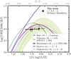 |
Fig. 5. Relation between the gas-phase metallicity measured using the direct Te−method and the R3 ratio. We compare our estimates with several strong-line metallicity calibrations from literature. We show the calibration by Bian et al. (2018), which uses local analogues that occupy similar regions to z ∼ 2 star-forming galaxies on the BPT diagram, the calibration based on local galaxies with EW(Hβ) ≥ 200 derived by Nakajima et al. (2022), Hirschmann et al. (2023) calibration for z > 4 galaxies from the TNG100 simulation, and Sanders et al. (2024) and Chakraborty et al. (2025) calibrations for high-z galaxies between 2 < z < 10. |
The uncertainties in our calculated gas temperatures and metallicities were calculated by perturbing the observed emission line luminosity values by their measured errors. We have 1000 realisations of the perturbation and calculated the median and the 16th and 84th percentile values.
4.2. Strong line calibration measurements
For our Hβ sample (5.5 ≤ z < 7), we do not cover the faint [O III]λ4364 auroral line. Therefore, we estimated the metallicity based on the R3 ratio using the Chakraborty et al. (2025) and Sanders et al. (2024) calibration recently derived for high-redshift galaxies, and the Nakajima et al. (2022) calibrations derived for high Hβ equivalent width galaxies (EW(Hβ)≥200 Å) in the local Universe (see Table 2). Our choice for these calibrations is validated by our direct-Te metallicity measurements for our Hγ sample (see Fig. 5). To obtain the metallicities for the Hβ sample, we solved the quadratic equation (cubic equation for Chakraborty et al. 2025) for the R3-calibrations iteratively, taking into account the observational error on the R3 ratio along with the errors on the calibration itself. We took the median of the solutions for the lower and higher branches to be the low and high metallicity estimate and the 16th and 84th percentile as the errors. As our spectra do not cover the [O II] emission lines, we cannot directly break the degeneracy between the ionisation parameter and the metallicity, which could both impact the [O III]λ5008/Hβ ratio. However, since our Hγ sample estimates fall either on the left branch or at the vertex of these relations, we assume that the galaxies in our Hβ sample also fall on the left branch of the calibrations, which corresponds to high ionisation and low metallicity. Our observations match best with the R3-calibration presented by Chakraborty et al. (2025), which is based on direct-Te metallicities for galaxies at 3 < z < 10. We discuss the impact of using strong-line calibrations in the next section.
Metallicity and SFR measurements in stellar mass bins for the Hβ (5.5 < z < 7) sample.
5. The mass-metallicity relation at z ∼ 6
Figure 6 shows the gas-phase oxygen abundances measured in our median stacked Hγ and Hβ sample along with other literature measurements. We find a positive correlation between gas-phase metallicity and stellar mass for both of our subsets. We parametrise the MZR as
 (4)
(4)
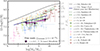 |
Fig. 6. Mass-metallicity relation from our stacked Hγ sample (purple stars, 6.3 ≤ z < 7). For the highest-mass bin in the Hβ sample, we also show the metallicity estimate from the higher-metallicity branch of the Sanders et al. (2024) R3-calibration curve (unfilled black star). The metallicity estimates and median stellar masses for both the samples are reported in Tables 1 and 2. The errors on the stellar mass were calculated using the 16th and 84th percentile values in the stack. While our measurements are from stellar-mass binned and stacked NIRCam grism spectra, similar to Li et al. (2025), measurements from Li et al. (2023) and He et al. (2024) were obtained using stacked spectra from NIRISS grism, measurements from Chakraborty et al. (2025), Chemerynska et al. (2024) and Pollock et al. (2025) are from individual galaxies, values from Curti et al. (2024) and Nakajima et al. (2023) are average metallicity measurements obtained from NIRSpec spectroscopy, and values from Faisst et al. (2025) were obtained from NIRSpec/IFU observations of high-mass main-sequence galaxies with [C II]158 μm observations from ALMA. |
where for the Hγ sample we find that the best-fit normalisation is Znorm = 7.96 ± 0.10, and the slope is γ = 0.12 ± 0.08. The parameters were obtained though orthogonal distance regression (ODR) using the scipy.odr package. Despite our lower sensitivity, our inferred metallicities agree with metallicity measurements, in similar redshift ranges, based on other surveys and instruments (e.g. NIRSpec MSA, Curti et al. 2024; Nakajima et al. 2023; Chakraborty et al. 2025).
Our MZR lies systematically below the MZR in the local Universe and those at z ∼ 2–3. It lies 0.72 dex below the MZR given by Scholte et al. (2024) for galaxies in the local Universe. At z ∼ 2, it lies 0.55 dex, 0.35 dex, and 0.61 dex below the MZR by Sanders et al. (2021), Li et al. (2023), and He et al. (2024), respectively. It lies 0.45 dex, 0.28 dex and 0.63 dex below the MZR at z ∼ 3 given by Sanders et al. (2021), Li et al. (2023), and He et al. (2024), respectively.
The normalisation of our Hγ sample MZR agrees with previous indications of redshift evolution in the MZR (Maiolino & Mannucci 2019; Curti 2025, and references therein). We find that the slope of our MZR for the Hγ sample agrees well with slopes found for a combined ‘green peas’ and ‘blueberries’ sample (Yang et al. 2017a,b) at z < 0.2, z = 2–3 galaxies by Li et al. (2023) using NIRISS grism, and the sample from the JADES survey at z = 6–10 (Curti et al. 2024). In standard gas regulator models, invariance in the slope of the MZR with an increase in redshift may suggest invariance in physical mechanisms driving outflows in star-forming galaxies, whereas the lowering of normalisation at fixed stellar mass at higher redshifts indicates inflow of pristine gas (Sanders et al. 2021; Heintz et al. 2023). Table B.1 presents the slope and normalisation for the MZR for our study and other works.
We also find that the slope of the MZR for the Hβ sample is flatter than that of our Hγ sample. As was described in previous sections, the metallicities for the Hβ sample were obtained from the lower branch of the Chakraborty et al. (2025), Sanders et al. (2024), and Nakajima et al. (2022) calibrations. The slope of the MZRs obtained using Chakraborty et al. (2025), Sanders et al. (2024), and Nakajima et al. (2022) calibrations are 0.10, 0.066, and 0.023 respectively, which are ∼0.03, 0.06, and 0.1 dex flatter than the slope of our direct-Te estimates. Our R3 ratios for the Hβ sample lie close to the vertex of the parabola, which can make the MZR appear flatter. Indeed, in Fig. 7, we show that calculating the metallicities of our Hγ sample stacks using the Chakraborty et al. (2025), Sanders et al. (2024), and Nakajima et al. (2022) calibrations significantly flattens the slope of the MZR compared to the MZR from direct-Te estimates. The general flatness of our MZR slope could also be due to the effects of our selection function, which we discuss in detail for the Hγ sample in Sect. 6.
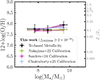 |
Fig. 7. Mass-metallicity relation inferred for our Hγ sample using the direct-Te method (purple stars), Chakraborty et al. (2025) R3-calibration (blue stars), Sanders et al. (2024) R3-calibration (magenta stars), and the Nakajima et al. (2022) R3-calibration for local galaxies with EW(Hβ) > 200 Å (green stars). We used metallicity estimates from the lower branch of the R3-calibrations. The use of strong-line methods leads to an artificial flattening of the observed relation. |
While there are studies that our MZR parameters agree with, the investigation of redshift evolution of the MZR is highly sensitive to systematic effects. For example, the best-fit parameters for our Hγ sample MZR compared to the MZR’s from other studies in the same redshift range differ due to discrepancies in the methods used to obtain gas-phase metallicities, different stellar mass ranges probed, different selection functions, and different parameters for SED fitting (He et al. 2024). Similarly, comparison of the MZR parameters for other redshift ranges is also affected by the same systematics. To understand the true evolution of the MZR, one should account for the selection effects for the various studies and estimate the metallicities using the same methodology. This is outside the scope of this work. However, we attempt to account for our observational selection and understand the nature of the intrinsic MZR in the section ahead.
6. Discussion
According to gas-regulator models, the slope of the MZR is governed by feedback mechanisms that drive gas out of galaxies (Peeples & Shankar 2011; Sanders et al. 2021; Curti et al. 2024). Such outflows are assumed to be driven by stellar feedback processes and are expected to be more effective in removing metal-enriched gas from lower-mass galaxies compared to high-mass ones due to their shallower gravitational potential wells. The normalisation is controlled by the ‘effective yield’ in the galaxy, which factors in the effect of nucleosynthetic stellar yields and gas flows. Finally, at fixed mass, the scatter along the MZR has been found to (anti-)correlate with the SFR of the galaxies. This has been observed as the FMR at z ∼ 0 (Mannucci et al. 2010; Lara-López et al. 2010; Andrews & Martini 2013; Curti et al. 2020). The existence of the FMR at high-z is still an unsolved question as many studies have shown that assuming the same FMR as at z ∼ 0 predicts higher metallicities than the ones they measure (Zahid et al. 2014; Salim et al. 2015; Kashino et al. 2017; Sanders et al. 2018; Heintz et al. 2023; Curti et al. 2024; Scholte et al. 2025; Korhonen Cuestas et al. 2025).
With recent results from JWST, new interpretations in understanding the MZR and FMR have arisen. JWST has shown that SFHs for high-z galaxies are usually bursty (Topping et al. 2022; Endsley et al. 2023; Looser et al. 2025). The burst of star formation may occur due to inflow of pristine gas, which dilutes the ISM, allowing for the galaxy to have a lower metallicity temporarily. However, there are other mechanisms through which the burst could occur (mergers, gravitational instabilities) that can cause an increase in the gas-phase metallicity (Tacchella et al. 2023). It has also been proposed that high-z galaxies have not yet reached a stage of equilibrium between gas accretion, star formation, chemical evolution, and feedback processes (Mannucci et al. 2010; Møller et al. 2013; Maiolino & Mannucci 2019; Curti et al. 2024; Sarkar et al. 2025; Scholte et al. 2025; Korhonen Cuestas et al. 2025). Evidence of a non-equilibrium state of the ISM in star-forming galaxies has been observed through studies of the circumgalactic medium (CGM) of Mg II absorption systems along the sight line of quasars at z ∼ 6 (Bordoloi et al. 2024) and also in terms of turbulent gas kinematics of high-z galaxies (Danhaive et al. 2025).
In the following sub-sections we discuss the implications of our measurements and investigate the impact of our selection function using simulations and mock datasets. It is noteworthy that having a selection function based on Hβ fluxes, instead of [O III]λ5008/Hβ fluxes, would also impose selection effects on the observed MZR due to the possibly interrelated nature of the 3D relation between stellar mass, SFR, and metallicity at these redshifts.
6.1. Comparison to cosmological simulations
The observed stellar masses of the galaxies in our Hγ sample span a range of log(M★/M⊙) = 6.9–10.5, with gas-phase metallicities ranging between Zgas = 7.7–8.0. We compared these measurements to those simulated in the SPHINX20 (Rosdahl et al. 2018; Katz et al. 2023) and FLARES (Lovell et al. 2020; Vijayan et al. 2020) hydrodynamical simulations, for which [O III] and Hβ luminosities are available. SPHINX20 is a cosmological hydrodynamical radiative transfer simulation with a volume of 203 cMpc3. The simulation was run down to z ≈ 4.5. The FLARES simulations are a suite of 40 zoom–re-simulations using the EAGLE model (Schaye et al. 2015; Crain et al. 2015), which has been shown to reproduce galaxy properties over a wide range of redshifts including z ≈ 0. The zoom regions were chosen to simulate a wide range of environments, from highly over-dense to under-dense. The FLARES simulations do not self-consistently model radiative transfer, but emission-line luminosities are added in post-processing based on Cloudy (version 17.03) modelling (Vijayan et al. 2020). For both simulations, we selected galaxies between z = 5–7 to compare to our dataset. We used the stellar masses, dust-attenuated emission-line luminosities, and mass-weighted gas-phase metallicities from these simulations. In our comparison, we also include JAGUAR (Williams et al. 2018), which is a mock galaxy catalogue based on observationally driven empirical models of the evolution of galaxy properties.
In Fig. 8, we show the MZR from FLARES, SPHINX20, and JAGUAR at z ∼ 6. We used the mass-weighted gas-phase metallicity from the SPHINX20 and FLARES simulation. Nakajima et al. (2023) make use of stellar metallicities of young star particles (< 10 Myr) from FLARES for comparison to their observations, assuming that the stellar and gas-phase metallicities in the region of massive star formation are comparable. We find that the slope (γ) and normalisation (Znorm) of the two MZRs from FLARES differ by 0.03 dex and 0.17 dex, respectively, with the MZR from stellar metallicities of young star particles being slightly steeper. From the JAGUAR catalogue, we used the gas-phase metallicities that were estimated using the Pettini & Pagel (2004) N2-metallicity calibration. We also plot our measurements based on the direct-Te method. We find that the simulations differ significantly. The slope and normalisation of the simulations, following Eq. (4), have been noted in Table B.1. The number of high-mass galaxies is limited in SPHINX20 and JAGUAR by the simulated volume. The low-mass cut-off determined by the resolution of the simulation, which is higher for SPHINX20, therefore includes lower-mass galaxies. At face value, our MZR is flatter than the one in FLARES and SPHINX20.
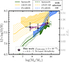 |
Fig. 8. Mass-metallicity relation for the SPHINX20 (Katz et al. 2023) and FLARES simulation (Lovell et al. 2020; Vijayan et al. 2020), and the JAGUAR catalogue (Williams et al. 2018). We plot both the intrinsic MZR and the MZR after mimicking our selection cut. We also show the MZR from our stacked Hγ (purple stars) sample. The MZR slopes and normalisations are listed in Table B.1. |
It is important to consider that our observational sample has been selected based on [O III] emission, the strength of which is sensitive to both SFR and metallicity, and therefore may yield a biased view of the MZR. In order to investigate the impact of our [O III]-flux limited galaxy sample on the observed MZR, we implemented our selection cut (f[O III]λ5008 ≥ 2 · 10−18 erg s−1 cm−2) on the [O III]λ5008 fluxes in these simulated datasets. Before comparing the impact of the selection function on the observed MZR, we first compare our observed the [O III] luminosity as a function of stellar mass to that in simulations. We find that FLARES and JAGUAR galaxies have roughly similar relations between [O III] luminosity and stellar mass as our observed data (see Appendix C). The SPHINX20 simulation, however, shows systematically higher masses at fixed [O III] luminosity, which stems from the fact that SPHINX20 has an elevated stellar-mass–halo-mass relation (i.e. galaxy formation is too efficient) and which therefore assigns too low SFRs (and consequently, [O III] luminosity) at fixed mass (Katz et al. 2023). As a result, after applying our selection cut, the SPHINX20 simulation only considers galaxies with log(M★/M⊙) > 8.4.
For the MZR, we find that our selection function causes the observed slope to be flatter in JAGUAR and SPHINX20 simulations. For JAGUAR, this is because our selection cut primarily removes low-metallicity galaxies at low masses. In SPHINX20, along with the selection described before, it primarily removes massive galaxies with relatively high metallicities. Both effects effectively lead to a flattening. Our [O III] selection does not affect the observed MZR slope from FLARES. As is discussed in the next section, the effect of the [O III] selection on the shape of the MZR depends on the correlation metallicity and the SFR at fixed mass. In FLARES, variations in metallicity are independent of SFR, such that the selection effect does not bias the observed shape of the MZR. The slopes for the [O III]-flux limited MZR are also summarised in Table B.1. We find a flatter MZR (slope, γ = 0.12 ± 0.08) from our Hγ sample as compared to SPHINX20 (γsel = 0.22) and FLARES (γsel = 0.44) MZR even after mimicking the selection cut in the simulations. Therefore, we conclude that none of these hydrodynamical simulations is able to match our observed MZR, in either the slope or the normalisation.
We note that the L[O III] − M★ relation from SPHINX20-pagination does not match our observations due to the low SFRs of SPHINX20 galaxies (see Appendix C). Since the gas-phase metallicity is inversely correlated to the sSFR in the simulation, our selection cut ends up selecting relatively high-metallicity galaxies and so the ‘observed’ MZR also does not match. In SPHINX20, we also miss out the highest-mass and highest-metallicity galaxies due to them being very dust-obscured, and thus not meeting our [O III] flux threshold. It is important to mention that we cannot account for missing out [O III]λλ4960, 5008 emitting galaxies in our observational data due to extreme dust-obscuration. This might contribute to the lack of a match between our observations and the simulations. There are no strong indications that we miss a large population of metal-enriched, dusty galaxies. For example, Rowland et al. (2025) observe the [O III] doublet for dusty galaxies at 6 < z < 8 with M★ > 109 M⊙ from the REBELS ALMA programme. Their sample is found to be more metal-rich than the bulk of the z > 6 population in the literature. However, we note that with their [O III] luminosities, such galaxies would have all been selected if they were covered by our observations.
6.2. Insights from modelling selection effects
Since the simulations do not match our observations and have varying responses to our selection function, we investigated the effects of our [O III] flux-limited selection function on the observed mass-metallicity relation using simple toy models. In these models we explore the various dependencies between metallicity and SFR at fixed stellar mass. We started by sampling the stellar masses for galaxies using the galaxy stellar mass function (SMF) from Weibel et al. (2024) at z = 6. Then, we assumed the following linear relation between SFR and the stellar mass that has been found by multiple observational studies (e.g. Speagle et al. 2014; Popesso et al. 2023):
 (5)
(5)
where the main-sequence slope is MSslope = 1.0 (motivated by the absence of strong evolution in the faint-end slope of the galaxy SMFs, Leja et al. 2015), the main-sequence normalisation is MSnorm = 2.0 (i.e. SFR = 100 M⊙/yr at log(M★/M⊙) = 10), and the intrinsic scatter along the relation is given by a normal distribution with standard deviation σSFR = 0.3 (as found in Di Cesare et al. 2025 for log(M★/M⊙) = 8). Additionally, we considered the following 3D relation between gas-phase metallicity, stellar mass, and SFR:
 (6)
(6)
where, Z0 is the normalisation, and Mcoeff and Scoeff are the coefficients that determine the dependency between metallicity on stellar mass and SFR (note that Mcoeff is not equal to the slope in the MZR due to the SFR dependence on mass). We then estimated Hβ luminosities for our mock galaxies considering case B recombination and using the SFR-LHα relation from Theios et al. (2019), which assumes a Kroupa IMF with upper mass cut-off of 100 M⊙ and slope −2.35 for M★ > 1 M⊙, and the BPASSv2.2 model with a constant SFH and a stellar metallicity of Z★ = 0.004. Finally, we obtained [O III]λ5008 luminosities using the calibration between the R3 ratio and gas-phase metallicity from Sanders et al. (2024).
Since we make various assumptions while generating the toy models, there are some caveats to keep in mind. Unlike our assumption, the scatter along the SFR-M★ relation may be mass-dependent, which would introduce a mass dependency in the scatter along the FMR. We also assumed a linear conversion between SFR and LHα as was prescribed by Theios et al. (2019), which has been assumed in the literature extensively, but which may not be the most optimal in the early Universe (Kramarenko et al. 2025). We assumed the R3 calibrations from Chakraborty et al. (2025), without any scatter, to get [O III]λ5008 luminosities. It is plausible that for a given metallicity and Hβ luminosity, there is scatter in this calibration that could be due to variations in the ionisation parameter. Finally, we ignored the effects of dust attenuation motivated by the low attenuation found in Sect. 3.5.
We generated mock datasets for three cases:
-
Normal FMR case (Scoeff < 0): There exists a 3D relation between the gas-phase metallicity, stellar mass, and SFR, such that gas-phase metallicity is inversely proportional to the specific star formation rate (sSFR). This is seen in galaxies in the local Universe and understood in the context of gas regulation models.
-
No FMR case (Scoeff = 0): In this scenario, there is no 3D relation between the gas-phase metallicity, stellar mass, and SFR. The gas-phase metallicity only depends on the stellar mass (MZR) and the scatter in the MZR is unrelated to SFR. This is the case in the FLARES simulation.
-
Inverted FMR case (Scoeff > 0): There exists a 3D relation between gas-phase metallicity, stellar mass, and SFR, but here gas-phase metallicity is directly proportional to the sSFR. This is seen on resolved (100 pc) scales in local galaxies (Wang & Lilly 2021) and suggests delayed or inefficient feedback.
The parameter choices for the three cases are given in Table 3. We motivate these three cases as they have a distinct impact on how our selection function influences the observed shape of the MZR. According to ‘gas-regulator models’, chemical enrichment in galaxies is set by an equilibrium between gas accretion, star formation, and outflows (Finlator & Davé 2008; Peeples & Shankar 2011; Davé et al. 2012; Lilly et al. 2013). Under such equilibrium, inflow of low-metallicity gas dilutes the ISM and triggers star formation. The star formation consumes the metal-poor gas and enriches the ISM, increasing the metallicity until new gas is accreted. This gives rise to the anti-correlated behaviour of the gas-phase metallicity and sSFR that has been observed by multiple observational studies in the local Universe as well in the early Universe (e.g. Mannucci et al. 2010; Lara-López et al. 2010; Sanders et al. 2018). This motivates the first case, the ‘normal’ FMR case, in our toy models. The parameter values for this case were taken from Andrews & Martini (2013), considering their 2D projection of the FMR. The scatter on Zgas comes from the scatter in the star-forming main sequence and strength of Scoeff (Eq. (5)).
However, it is unclear whether the normal FMR evolves out to high redshift as multiple studies have also found discrepancies in their observations (Zahid et al. 2014; Heintz et al. 2023; Curti et al. 2024; Scholte et al. 2025; Cullen et al. 2025). In a recent study, Laseter et al. (2025) find no evidence of the existence of the normal FMR at z ∼ 0 for the low-M★ regime, indicating a deviation from the equilibrium conditions as seen at the higher-M★ regime. While the gas-regulator models explain the existence of FMR, there are many caveats. For example, supernovae outflows are the only feedback assumed in the models. Additionally, these models assume time-invariant star-forming efficiencies, which may not be true for galaxies with bursty SFHs. Importantly, the 3D relation is not just set by the strengths of processes such as the mass inflow rate, SFR, mass loading factor, ISM metallicity, effective yields, and star forming efficiency, but also by the timescales of their variations (Torrey et al. 2018; Wang & Lilly 2021). Torrey et al. (2018) show that if the timescales of variations in the SFR and gas-phase metallicity are within a factor of ∼1.5 of each other in the TNG100 simulation, then the normal FMR case should hold. However, if either the SFR or metallicity evolves much faster than the other it can either wash out any correlation between them or cause a positive correlation. This motivates our second case (no FMR) and third case (inverted FMR). Processes such as bursty star formation can significantly impact the variability of the SFR, while not impacting the metallicity much. Multiple studies have shown evidence of bursty star formation for high-redshift galaxies (Topping et al. 2022; Endsley et al. 2023; Looser et al. 2025). Additionally, variability in processes such as a temporary increase in the SFE due to gravitational instabilities, or an increase in outflows with the same metallicity as the ISM, can allow for a positive correlation between the sSFR and gas-phase metallicity (Torrey et al. 2018; Wang & Lilly 2021). Indications of an ‘inverted’ FMR have also been seen in the THESAN-ZOOM simulation for galaxies with log(M★/M⊙)≲9 due to regular inflow of low-metallicity gas (McClymont et al. 2025). The parameters for the second case (No FMR) were taken from the MZR presented in Curti et al. (2024). We assumed a scatter of 0.1 dex on the MZR. For the third case, we obtained the parameters for Eq. (6) by matching the shape of the intrinsic MZR to the one obtained considering the normal FMR case. We kept the Scoeff to be the same magnitude as in the normal FMR case and only changed the sign. In this case, we find Mcoeff < 0. As per Eq. (6), this does not imply a negative correlation between metallicity and stellar mass as SFR is also a function of stellar mass (see Appendix D). However, this does point towards processes such as bursty star formation and inflow of pristine gas being more dominant compared to the stellar mass at high redshift.
In the top panel of Fig. 9, we show the distribution of simulated galaxies on the mass-metallicity plane for the three cases mentioned above. We apply our selection cut to the [O III]λ5008 luminosity. We then compare how the MZR of the selected sample, i.e. the observable MZR, compares to the intrinsic one. The selection cut affects the three cases differently. In case 1 (normal FMR), the observable MZR is steeper than the intrinsic MZR. In this case, Zgas ∝ 1/sSFR, an [O III] flux cut therefore selects galaxies with a lower metallicity. This makes the slope of the observable MZR steeper. In case 2 (No FMR), there is negligible change in the intrinsic MZR and the observable MZR slopes. The small change in the slope can be attributed to the scatter added to the MZR. In case 3 (inverted FMR), the observable MZR is flatter than the intrinsic MZR. In this case, Zgas ∝ sSFR, the [O III] flux thus scales with SFR, and we end up selecting galaxies with higher metallicities with an [O III] flux cut. This makes the slope of the observable MZR flatter.
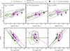 |
Fig. 9. Top: MZR for the three cases in our toy model. We also plot our direct-Te metallicity estimates. Bottom: Specific star formation rate (sSFR) as a function of gas-phase metallicity. We show sSFR vs. gas-phase metallicity for our Hγ stellar mass binned stacks. The error bars on the sSFR were calculated using the 16th and 84th percentile in the stacks. The top left and bottom left panels show Case 1 (‘normal FMR’). Our selection cut makes the MZR slope steeper. The top middle and bottom middle panels show Case 2 (‘no FMR’). Our selection cut does not affect the MZR slope. The top right and bottom middle panels show Case 3 (‘inverted FMR’). Our selection cut makes the MZR slope appear flatter. In all three cases, we find a negative correlation between sSFR and 12+log(O/H) upon implementing our selection cut. |
With the data currently available, it is not possible to determine which scenario our observations follow as there are multiple degeneracies in the free parameters while evaluating the metallicities using Eq. (6) (we discuss these degeneracies in Appendix D). We attempted to test which scenario explains our observations by studying the sSFR as a function of the gas-phase metallicity, as is shown in the bottom panel of Fig. 9. We see a negative correlation between the sSFR and gas-phase metallicity for both the ‘intrinsic’ and ‘observable’ distribution in case 1. In case 2, there is no correlation between the sSFR and gas-phase metallicity for the intrinsic distribution; however, on application of our selection cut we find a negative correlation. In case 3, both the intrinsic and observable distributions have a positive correlation. We find a negative correlation in our observations, the slope of which is best represented by the ‘no FMR’ case. This suggests an absent or weak (Scoeff = 0 or |Scoeff|< < 1 but ≠ 0) FMR at z ∼ 6, which may allude to the galaxies at these redshifts being out of equilibrium, as has been suggested previously for high-redshift galaxies (Maiolino & Mannucci 2019; Bordoloi et al. 2024; Danhaive et al. 2025). In addition to the MZR parameters from Curti et al. (2024) for case 2, we also explored the impact of using parameters from other MZRs in the literature (Heintz et al. 2023; Sarkar et al. 2025, see our Appendix E). We find that our observations generally agree with the MZR models in the sSFR versus gas-phase metallicity plane. If this is the true underlying scenario, then our intrinsic slope is as flat as our observed slope, which points towards either rapid metal enrichment in low-mass galaxies or lower metallicities due to pristine gas inflows in higher-mass galaxies. Previous observations of high-z galaxies are not in favour of lower metallicities for high-stellar-mass galaxies (Rowland et al. 2025), suggesting the former explanation. Observations of CGM galaxies at z ∼ 6 also indicate that galaxies in the early Universe were efficient in chemically enriching their surroundings (Bordoloi et al. 2024).
In this case, it is important to note that a good fit between the model and the data does not necessarily indicate that the intrinsic trend is represented by the model. Figure 9 shows that the scatter in the sSFR-metallicity relation varies across models. Additionally, Fig. E.1 shows that scatter even varies in the sSFR-metallicity plane for the same model (case 2, Scoeff = 0) with different parameters. Therefore to fit the parameters and distinguish between the models, we need to fit the scatter. Due to the stacked measurements of the metallicity, we cannot measure the scatter in the sSFR – metallicity relation, and therefore cannot fully constrain the SFR dependence. To do this we require observations with robust metallicity measurements for a statistically large sample of individual galaxies with a well-defined selection function, as this crucially impacts the observed relations.
7. Summary
In this work, we have studied and characterised the MZR and the 3D correlation between the stellar mass, gas-phase metallicity, and SFR, dubbed the FMR, of [O III] selected galaxies with redshifts between 5 < z < 7. We obtained the spectra for these galaxies using deep NIRCam WFSS surveys, EIGER (Kashino et al. 2023), COLA1 (Torralba-Torregrosa et al. 2024), and ALT (Naidu et al. 2024). Grism spectra have a well-understood flux-limited selection function and are not subject to slit losses. To make the selection uniform across the data from the three surveys uniform, we made a conservative [O III] flux cut, f[O III]λ5008 ≥ 2 × 10⁻¹⁸ erg s−1 cm−2. Since grism spectra are less sensitive and have a smaller wavelength coverage compared to NIRSpec spectra, we performed stacking in stellar mass bins to detect faint emission lines such as [O III]λ4364 and Hγ with a S/N > 3 (see Fig. 3). This allowed us to derive direct-Te-based metallicities for our analysis. We tested the impact of our selection function using hydrodynamical simulations such as FLARES (Lovell et al. 2020; Vijayan et al. 2020) and SPHINX20 (Rosdahl et al. 2018; Katz et al. 2023) and the JAGUAR catalogue (Williams et al. 2018). We further tested our selection function using simple toy models for three scenarios: (1) normal FMR (Zgas ∝ 1/sSFR), (2) no FMR (no SFR dependence), and (3) inverted FMR (Zgas ∝ sSFR). Our main results are:
-
We cover Hγ and [O III]λ4363 for a sample of 270 galaxies (i.e. the Hγ sample). We detect Hγ, [O III]λ4363, Hβ and [O III]λ4960, 5008 when stacking in bins of stellar mass, which allows us to measure direct-Te metallicities in the stacks. The observed stellar masses for this sample span a range of log(M★/M⊙) = 6.9–10.5, with the gas-phase metallicities ranging between Zgas = 7.7–8.0 (0.11–0.22 Z⊙) [Sect. 4.1, Fig. 6, Table 1].
-
With the measured direct-Te metallicities, we tested the R3 calibration curve for high-z galaxies. We found that our direct-Te measurements are slightly offset to higher values of the R3 ratio at fixed metallicity compared to the R3 calibration curves from Sanders et al. (2024) and Nakajima et al. (2022). However, within the observational errors and the errors on the calibration itself, our values agree with these curves [Sect. 4.2, Fig. 5].
-
We obtain a linear MZR relation with normalisation Znorm = 7.96 ± 0.08 and slope γ = 0.12 ± 0.08 for the direct-Te measurements from the Hγ sample [Sect. 5, Eq. (4)]. The MZR lies systematically below the MZR measured for galaxies in the local Universe (Scholte et al. 2024) and at z ∼ 2–3 (Sanders et al. 2021; Li et al. 2023). The slope of our MZR agrees well with those found for analogues at lower redshift (Yang et al. 2017a,b) and with other z = 6–10 measurements (Curti et al. 2024; see our Sect. 5, Fig. 6, and Table B.1).
-
We find that our measurements do not match the slope and normalisation of the MZR of galaxies in the FLARES and SPHINX20 simulations and the JAGUAR model. The observed slope is significantly shallower, which is robust to our selection effects. Selection effects impact simulations non-uniformly. In SPHINX20 and JAGUAR, on applying the selection cut, the MZR becomes flatter. For FLARES, there is no change in the MZR upon application of the selection cut (Sect. 6.1, Fig. 8, and Table B.1).
-
Through simple toy models, we show that the effect of our [O III] selection cut on the MZR depends on the relation between gas-phase metallicity and sSFR of the galaxies. In the case of a normal FMR, the observable MZR (after the selection cut) is steeper than the intrinsic MZR. In the case of no FMR, i.e. no SFR dependence, there is negligible change in the intrinsic MZR and the observable MZR slopes. In the case of an inverted FMR, the observable MZR is flatter than the intrinsic MZR [Sect. 6.2, Fig. 9, Table 3]. Our data agrees well with the no FMR case. This suggests an absent or weak FMR at z ∼ 6, which is similar to what we find in FLARES. An absent or weak FMR points towards the possibility that the galaxies at these redshifts are not yet in equilibrium. A no FMR case would imply that the intrinsic slope of the MZR is as flat as the observed one. Such flatness may be due to rapid metal enrichment [Sect. 6.2, Fig. 9]. However, since our data points were obtained through stacking, they are not enough to constrain the scatter in the three cases and therefore distinguish cleanly among them.
This work highlights the importance of accounting for selection functions in order understand the physics underlying scaling relations such as the MZR and the FMR. In order to understand the baryon cycle in depth at high redshifts, future observations with robust metallicity measurements are required for statistically large well-defined samples of galaxies.
Acknowledgments
We thank the anonymous referee for the insightful comments that helped improving this paper. This work is based on observations made with the NASA/ESA/CSA James Webb Space Telescope. The data were obtained from the Mikulski Archive for Space Telescopes at the Space Telescope Science Institute, which is operated by the Associations of Universities for Research in Astronomy, Inc., under NASA contract NAS 5-03127 for JWST. These observations were taken under programmes # 1243, # 1933 and # 3516. Funded by the European Union (ERC, AGENTS, 101076224). Views and opinions expressed are however those of the author(s) only and do not necessarily reflect those of the European Union or the European Research Council. Neither the European Union nor the granting authority can be held responsible for them. GK acknowledges support from the Foundation MERAC. APV acknowledge support from the Sussex Astronomy Centre STFC Consolidated Grant (ST/X001040/1).
References
- Andrews, B. H., & Martini, P. 2013, ApJ, 765, 140 [NASA ADS] [CrossRef] [Google Scholar]
- Bezanson, R., Labbe, I., Whitaker, K. E., et al. 2024, ApJ, 974, 92 [NASA ADS] [CrossRef] [Google Scholar]
- Bian, F., Kewley, L. J., & Dopita, M. A. 2018, ApJ, 859, 175 [CrossRef] [Google Scholar]
- Bordoloi, R., Simcoe, R. A., Matthee, J., et al. 2024, ApJ, 963, 28 [NASA ADS] [CrossRef] [Google Scholar]
- Bothwell, M. S., Maiolino, R., Kennicutt, R., et al. 2013, MNRAS, 433, 1425 [Google Scholar]
- Bothwell, M. S., Maiolino, R., Cicone, C., Peng, Y., & Wagg, J. 2016, A&A, 595, A48 [NASA ADS] [CrossRef] [EDP Sciences] [Google Scholar]
- Bradley, L., Sipőcz, B., Robitaille, T., et al. 2024, https://doi.org/10.5281/zenodo.13989456 [Google Scholar]
- Brooks, M., Simons, R. C., Trump, J. R., et al. 2025, ApJ, 986, 177 [Google Scholar]
- Cameron, A. J., Saxena, A., Bunker, A. J., et al. 2023, A&A, 677, A115 [NASA ADS] [CrossRef] [EDP Sciences] [Google Scholar]
- Cardelli, J. A., Clayton, G. C., & Mathis, J. S. 1989, ApJ, 345, 245 [Google Scholar]
- Cataldi, E., Belfiore, F., Curti, M., et al. 2025, A&A, 703, A208 [NASA ADS] [CrossRef] [EDP Sciences] [Google Scholar]
- Chabrier, G. 2003, PASP, 115, 763 [Google Scholar]
- Chakraborty, P., Sarkar, A., Smith, R., et al. 2025, ApJ, 985, 24 [Google Scholar]
- Chemerynska, I., Atek, H., Dayal, P., et al. 2024, ApJ, 976, L15 [NASA ADS] [CrossRef] [Google Scholar]
- Choi, J., Dotter, A., Conroy, C., et al. 2016, ApJ, 823, 102 [Google Scholar]
- Conroy, C., & Gunn, J. E. 2010, ApJ, 712, 833 [Google Scholar]
- Conroy, C., Gunn, J. E., & White, M. 2009, ApJ, 699, 486 [Google Scholar]
- Crain, R. A., Schaye, J., Bower, R. G., et al. 2015, MNRAS, 450, 1937 [NASA ADS] [CrossRef] [Google Scholar]
- Cresci, G., Mannucci, F., Sommariva, V., et al. 2012, MNRAS, 421, 262 [NASA ADS] [Google Scholar]
- Cullen, F., Carnall, A. C., Scholte, D., et al. 2025, MNRAS, 540, 2176 [Google Scholar]
- Curti, M. 2025, arXiv e-prints [arXiv:2504.08933] [Google Scholar]
- Curti, M., Mannucci, F., Cresci, G., & Maiolino, R. 2020, MNRAS, 491, 944 [Google Scholar]
- Curti, M., Maiolino, R., Curtis-Lake, E., et al. 2024, A&A, 684, A75 [NASA ADS] [CrossRef] [EDP Sciences] [Google Scholar]
- Danhaive, A. L., Tacchella, S., Übler, H., et al. 2025, MNRAS, 543, 3249 [Google Scholar]
- Davé, R., Finlator, K., & Oppenheimer, B. D. 2012, MNRAS, 421, 98 [Google Scholar]
- Dayal, P., Ferrara, A., & Dunlop, J. S. 2013, MNRAS, 430, 2891 [Google Scholar]
- De Rossi, M. E., Bower, R. G., Font, A. S., Schaye, J., & Theuns, T. 2017, MNRAS, 472, 3354 [Google Scholar]
- Di Cesare, C., Matthee, J., Naidu, R. P., et al. 2025, A&A, accepted [arXiv:2510.19044] [Google Scholar]
- Dotter, A. 2016, ApJS, 222, 8 [Google Scholar]
- Ellison, S. L., Patton, D. R., Simard, L., & McConnachie, A. W. 2008, ApJ, 672, L107 [NASA ADS] [CrossRef] [Google Scholar]
- Endsley, R., Stark, D. P., Whitler, L., et al. 2023, MNRAS, 524, 2312 [NASA ADS] [CrossRef] [Google Scholar]
- Faisst, A. L., Liu, L.-J., Dubois, Y., et al. 2025, arXiv e-prints [arXiv:2510.16106] [Google Scholar]
- Ferland, G. J., Korista, K. T., Verner, D. A., et al. 1998, PASP, 110, 761 [Google Scholar]
- Ferland, G. J., Porter, R. L., van Hoof, P. A. M., et al. 2013, Rev. Mex. Astron. Astrofis., 49, 137 [Google Scholar]
- Finlator, K., & Davé, R. 2008, MNRAS, 385, 2181 [NASA ADS] [CrossRef] [Google Scholar]
- Furtak, L. J., Zitrin, A., Weaver, J. R., et al. 2023, MNRAS, 523, 4568 [NASA ADS] [CrossRef] [Google Scholar]
- Hahn, C., Wilson, M. J., Ruiz-Macias, O., et al. 2023, AJ, 165, 253 [CrossRef] [Google Scholar]
- He, X., Wang, X., Jones, T., et al. 2024, ApJ, 960, L13 [Google Scholar]
- Heintz, K. E., Brammer, G. B., Giménez-Arteaga, C., et al. 2023, Nat. Astron., 7, 1517 [NASA ADS] [CrossRef] [Google Scholar]
- Hirschmann, M., Charlot, S., & Somerville, R. S. 2023, MNRAS, 526, 3504 [NASA ADS] [CrossRef] [Google Scholar]
- Horne, K. 1986, PASP, 98, 609 [Google Scholar]
- Isobe, Y., Ouchi, M., Nakajima, K., et al. 2023, ApJ, 956, 139 [NASA ADS] [CrossRef] [Google Scholar]
- Izotov, Y. I., Stasińska, G., Meynet, G., Guseva, N. G., & Thuan, T. X. 2006, A&A, 448, 955 [CrossRef] [EDP Sciences] [Google Scholar]
- Johnson, B. D., Leja, J., Conroy, C., & Speagle, J. S. 2021, ApJS, 254, 22 [NASA ADS] [CrossRef] [Google Scholar]
- Kashino, D., Silverman, J. D., Sanders, D., et al. 2017, ApJ, 835, 88 [NASA ADS] [CrossRef] [Google Scholar]
- Kashino, D., Lilly, S. J., Matthee, J., et al. 2023, ApJ, 950, 66 [CrossRef] [Google Scholar]
- Kashino, D., Lilly, S. J., Matthee, J., et al. 2025, arXiv e-prints [arXiv:2506.03121] [Google Scholar]
- Katz, H., Rosdahl, J., Kimm, T., et al. 2023, Open J. Astrophys., 6, 44 [NASA ADS] [CrossRef] [Google Scholar]
- Kewley, L. J., Nicholls, D. C., & Sutherland, R. S. 2019, ARA&A, 57, 511 [Google Scholar]
- Korhonen Cuestas, N. A., Strom, A. L., Miller, T. B., et al. 2025, ApJ, 984, 188 [Google Scholar]
- Kramarenko, I. G., Rosdahl, J., Blaizot, J., et al. 2025, A&A, submitted [arXiv:2509.05403] [Google Scholar]
- Kriek, M., Shapley, A. E., Reddy, N. A., et al. 2015, ApJS, 218, 15 [NASA ADS] [CrossRef] [Google Scholar]
- Lara-López, M. A., Cepa, J., Bongiovanni, A., et al. 2010, A&A, 521, L53 [CrossRef] [EDP Sciences] [Google Scholar]
- Laseter, I. H., Maseda, M. V., Curti, M., et al. 2024, A&A, 681, A70 [NASA ADS] [CrossRef] [EDP Sciences] [Google Scholar]
- Laseter, I. H., Maseda, M. V., Bunker, A. J., et al. 2025, arXiv e-prints [arXiv:2510.15024] [Google Scholar]
- Leja, J., van Dokkum, P. G., Franx, M., & Whitaker, K. E. 2015, ApJ, 798, 115 [NASA ADS] [CrossRef] [Google Scholar]
- Li, M., Cai, Z., Bian, F., et al. 2023, ApJ, 955, L18 [CrossRef] [Google Scholar]
- Li, Z., Kakiichi, K., Christensen, L., et al. 2025, A&A, 703, A106 [NASA ADS] [CrossRef] [EDP Sciences] [Google Scholar]
- Lilly, S. J., Carollo, C. M., Pipino, A., Renzini, A., & Peng, Y. 2013, ApJ, 772, 119 [NASA ADS] [CrossRef] [Google Scholar]
- Looser, T. J., D’Eugenio, F., Maiolino, R., et al. 2025, A&A, 697, A88 [NASA ADS] [CrossRef] [EDP Sciences] [Google Scholar]
- Lovell, C. C., Vijayan, A. P., Thomas, P. A., et al. 2020, MNRAS, 500, 2127 [NASA ADS] [CrossRef] [Google Scholar]
- Luridiana, V., Morisset, C., & Shaw, R. A. 2013, Astrophysics Source Code Library [record ascl:1304.021] [Google Scholar]
- Ma, C., Wang, K., Wang, E., et al. 2024, ApJ, 971, L14 [Google Scholar]
- Mahabal, A., Stern, D., Bogosavljević, M., Djorgovski, S. G., & Thompson, D. 2005, ApJ, 634, L9 [NASA ADS] [CrossRef] [Google Scholar]
- Maier, C., Ziegler, B. L., Lilly, S. J., et al. 2015, A&A, 577, A14 [NASA ADS] [CrossRef] [EDP Sciences] [Google Scholar]
- Maiolino, R., & Mannucci, F. 2019, A&ARv, 27, 3 [Google Scholar]
- Maiolino, R., Nagao, T., Grazian, A., et al. 2008, A&A, 488, 463 [NASA ADS] [CrossRef] [EDP Sciences] [Google Scholar]
- Mannucci, F., Cresci, G., Maiolino, R., et al. 2009, MNRAS, 398, 1915 [Google Scholar]
- Mannucci, F., Cresci, G., Maiolino, R., Marconi, A., & Gnerucci, A. 2010, MNRAS, 408, 2115 [NASA ADS] [CrossRef] [Google Scholar]
- Marino, R. A., Rosales-Ortega, F. F., Sánchez, S. F., et al. 2013, A&A, 559, A114 [NASA ADS] [CrossRef] [EDP Sciences] [Google Scholar]
- Matthee, J., Sobral, D., Gronke, M., et al. 2018, A&A, 619, A136 [NASA ADS] [CrossRef] [EDP Sciences] [Google Scholar]
- Matthee, J., Mackenzie, R., Simcoe, R. A., et al. 2023, ApJ, 950, 67 [NASA ADS] [CrossRef] [Google Scholar]
- Matthee, J., Naidu, R. P., Brammer, G., et al. 2024, ApJ, 963, 129 [NASA ADS] [CrossRef] [Google Scholar]
- McClymont, W., Tacchella, S., Smith, A., et al. 2025, arXiv e-prints [arXiv:2507.08787] [Google Scholar]
- Møller, P., Fynbo, J. P. U., Ledoux, C., & Nilsson, K. K. 2013, MNRAS, 430, 2680 [CrossRef] [Google Scholar]
- Morishita, T., Stiavelli, M., Grillo, C., et al. 2024, ApJ, 971, 43 [NASA ADS] [CrossRef] [Google Scholar]
- Moustakas, J., Zaritsky, D., Brown, M., et al. 2011, arXiv e-prints [arXiv:1112.3300] [Google Scholar]
- Naidu, R. P., Oesch, P. A., van Dokkum, P., et al. 2022, ApJ, 940, L14 [NASA ADS] [CrossRef] [Google Scholar]
- Naidu, R. P., Matthee, J., Kramarenko, I., et al. 2024, arXiv e-prints [arXiv:2410.01874] [Google Scholar]
- Nakajima, K., Ouchi, M., Xu, Y., et al. 2022, ApJS, 262, 3 [CrossRef] [Google Scholar]
- Nakajima, K., Ouchi, M., Isobe, Y., et al. 2023, ApJS, 269, 33 [NASA ADS] [CrossRef] [Google Scholar]
- Oke, J. B., & Gunn, J. E. 1983, ApJ, 266, 713 [NASA ADS] [CrossRef] [Google Scholar]
- Osterbrock, D. E., & Ferland, G. J. 2006, Astrophysics of Gaseous Nebulae and Active Galactic Nuclei [Google Scholar]
- Peeples, M. S., & Shankar, F. 2011, MNRAS, 417, 2962 [NASA ADS] [CrossRef] [Google Scholar]
- Pettini, M., & Pagel, B. E. J. 2004, MNRAS, 348, L59 [NASA ADS] [CrossRef] [Google Scholar]
- Planck Collaboration VI. 2020, A&A, 641, A6 [NASA ADS] [CrossRef] [EDP Sciences] [Google Scholar]
- Pollock, C. L., Gottumukkala, R., Heintz, K. E., et al. 2025, A&A, submitted [arXiv:2506.15779] [Google Scholar]
- Popesso, P., Concas, A., Cresci, G., et al. 2023, MNRAS, 519, 1526 [Google Scholar]
- Price, S. H., Bezanson, R., Labbe, I., et al. 2025, ApJ, 982, 51 [Google Scholar]
- Roberts-Borsani, G., Treu, T., Shapley, A., et al. 2024, ApJ, 976, 193 [NASA ADS] [CrossRef] [Google Scholar]
- Rosdahl, J., Katz, H., Blaizot, J., et al. 2018, MNRAS, 479, 994 [NASA ADS] [Google Scholar]
- Rowland, L. E., Stefanon, M., Bouwens, R., et al. 2025, arXiv e-prints [arXiv:2501.10559] [Google Scholar]
- Salim, S., Lee, J. C., Davé, R., & Dickinson, M. 2015, ApJ, 808, 25 [NASA ADS] [CrossRef] [Google Scholar]
- Sanders, R. L., Shapley, A. E., Kriek, M., et al. 2016, ApJ, 816, 23 [Google Scholar]
- Sanders, R. L., Shapley, A. E., Kriek, M., et al. 2018, ApJ, 858, 99 [NASA ADS] [CrossRef] [Google Scholar]
- Sanders, R. L., Shapley, A. E., Jones, T., et al. 2021, ApJ, 914, 19 [CrossRef] [Google Scholar]
- Sanders, R. L., Shapley, A. E., Topping, M. W., Reddy, N. A., & Brammer, G. B. 2024, ApJ, 962, 24 [NASA ADS] [CrossRef] [Google Scholar]
- Sarkar, A., Chakraborty, P., Vogelsberger, M., et al. 2025, ApJ, 978, 136 [Google Scholar]
- Schaye, J., Crain, R. A., Bower, R. G., et al. 2015, MNRAS, 446, 521 [Google Scholar]
- Scholte, D., Saintonge, A., Moustakas, J., et al. 2024, MNRAS, 535, 2341 [Google Scholar]
- Scholte, D., Cullen, F., Carnall, A. C., et al. 2025, MNRAS, 540, 1800 [Google Scholar]
- Shapley, A. E., Coil, A. L., Ma, C.-P., & Bundy, K. 2005, ApJ, 635, 1006 [CrossRef] [Google Scholar]
- Speagle, J. S., Steinhardt, C. L., Capak, P. L., & Silverman, J. D. 2014, ApJS, 214, 15 [Google Scholar]
- Suess, K. A., Weaver, J. R., Price, S. H., et al. 2024, ApJ, 976, 101 [Google Scholar]
- Tacchella, S., Finkelstein, S. L., Bagley, M., et al. 2022, ApJ, 927, 170 [NASA ADS] [CrossRef] [Google Scholar]
- Tacchella, S., Johnson, B. D., Robertson, B. E., et al. 2023, MNRAS, 522, 6236 [NASA ADS] [CrossRef] [Google Scholar]
- Theios, R. L., Steidel, C. C., Strom, A. L., et al. 2019, ApJ, 871, 128 [NASA ADS] [CrossRef] [Google Scholar]
- Topping, M. W., Shapley, A. E., Sanders, R. L., et al. 2021, MNRAS, 506, 1237 [CrossRef] [Google Scholar]
- Topping, M. W., Stark, D. P., Endsley, R., et al. 2022, ApJ, 941, 153 [NASA ADS] [CrossRef] [Google Scholar]
- Topping, M. W., Sanders, R. L., Shapley, A. E., et al. 2025, MNRAS, 541, 1707 [Google Scholar]
- Torralba-Torregrosa, A., Matthee, J., Naidu, R. P., et al. 2024, A&A, 689, A44 [NASA ADS] [CrossRef] [EDP Sciences] [Google Scholar]
- Torrey, P., Vogelsberger, M., Hernquist, L., et al. 2018, MNRAS, 477, L16 [Google Scholar]
- Torrey, P., Vogelsberger, M., Marinacci, F., et al. 2019, MNRAS, 484, 5587 [NASA ADS] [Google Scholar]
- Tremonti, C. A., Heckman, T. M., Kauffmann, G., et al. 2004, ApJ, 613, 898 [Google Scholar]
- Vijayan, A. P., Lovell, C. C., Wilkins, S. M., et al. 2020, MNRAS, 501, 3289 [Google Scholar]
- Wang, E., & Lilly, S. J. 2021, ApJ, 910, 137 [NASA ADS] [CrossRef] [Google Scholar]
- Weibel, A., Oesch, P. A., Barrufet, L., et al. 2024, MNRAS, 533, 1808 [NASA ADS] [CrossRef] [Google Scholar]
- Whitler, L., Stark, D. P., Endsley, R., et al. 2023, MNRAS, 519, 5859 [NASA ADS] [CrossRef] [Google Scholar]
- Williams, C. C., Curtis-Lake, E., Hainline, K. N., et al. 2018, ApJS, 236, 33 [CrossRef] [Google Scholar]
- Wuyts, E., Kurk, J., Förster Schreiber, N. M., et al. 2014, ApJ, 789, L40 [NASA ADS] [CrossRef] [Google Scholar]
- Yabe, K., Ohta, K., Akiyama, M., et al. 2015, PASJ, 67, 102 [NASA ADS] [CrossRef] [Google Scholar]
- Yang, H., Malhotra, S., Gronke, M., et al. 2017a, ApJ, 844, 171 [NASA ADS] [CrossRef] [Google Scholar]
- Yang, H., Malhotra, S., Rhoads, J. E., & Wang, J. 2017b, ApJ, 847, 38 [NASA ADS] [CrossRef] [Google Scholar]
- York, D. G., Adelman, J., Anderson, J. E., Jr., et al. 2000, AJ, 120, 1579 [NASA ADS] [CrossRef] [Google Scholar]
- Zahid, H. J., Kashino, D., Silverman, J. D., et al. 2014, ApJ, 792, 75 [NASA ADS] [CrossRef] [Google Scholar]
Wavelengths around the Lyman-α line are ignored in the SED fitting because of uncertainty in the IGM attenuation.
The Bayesian information criterion (BIC) values of the Voigt profiles for the [O III]λ4960, 5008 doublet with the same standard deviation and Gamma parameter values and a fixed emission-line ratio are significantly lower than the BIC values for Gaussian profiles with the same standard deviation and fixed emission-line ratio. The absolute difference in the BIC values is larger than 10, with the BIC values for the Voigt profiles being lower. Therefore, a Voigt profile is preferred.
Appendix A: Metallicity estimates for Hβ sample using R3-calibrations
We report the gas-phase metallicity estimates for our stellar mass bin stacked Hβ sample using the R3-calibrations presented in Nakajima et al. (2022) and Sanders et al. (2024) in Table A.1. We use R3-calibration presented for local galaxies with EWHβ ≥ 200 from Nakajima et al. (2022). The gas-phase metallicities have been estimated using the same methodology as described in Sect. 4.2.
Gas-phase metallicity estimates in stellar mass bins for the Hβ (5.5 < z < 7) sample using R3 calibration.
Appendix B: MZR parameters for observations and simulations
We report the slope and normalisation for the MZR for our direct-Te measurements along with the observational samples and simulations, following Eq. 4. For the simulations, we present the MZR parameters for a sample with the same selection cut as our observations (i.e. an [O III]-flux cut) and for a sample without any selection cut.
Slope of the MZR in various observational samples and in simulations.
Appendix C: The relation between [O III]λ5008 luminosity and stellar mass
Before assessing the impact of our line-flux limited selection function on the mass - metallicity relation, it is important to compare the relation between the [O III] line luminosity and stellar mass among simulations and observations. In Fig. C.1, we show [O III]λ5008 luminosity as a function of stellar masses for Hβ and Hγ sample, as well as for the hydrodynamical simulations SPHINX20 and FLARES, and the JAGUAR catalogue. Upon applying our selection cut to these simulations, we find that the FLARES simulation and the JAGUAR catalogue match our relation between stellar mass and [O III] luminosities very well. The intrinsic relations are significantly steeper than observed, but this can be understood as being due to the selection cut. In SPHINX20 however, only galaxies above stellar mass of 108.4 M⊙ are selected with the [O III] flux threshold. As mentioned in Sect. 6.1, SPHINX20 has an elevated stellar mass - halo mass relation and therefore assigns too low SFRs at fixed mass, leading to much lower [OIII] luminosities at all masses.
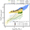 |
Fig. C.1. [O III]λ5008 luminosities as a function of stellar mass for the SPHINX20 (Katz et al. 2023) and FLARES simulation (Lovell et al. 2020; Vijayan et al. 2020), the JAGUAR catalogue (Williams et al. 2018). We plot both, the intrinsic relation and the relation after mimicking our selection cut. We also show the L[O III]λ5008−log(M★/M⊙) relation for our stacked Hγ (purple stars) and Hβ (orange stars) sample. |
Appendix D: Derivation of the FMR equation used in our toy model
In in Sect. 6.2, we describe our toy models used to understand the impact of the 3D relation between metallicity-stellar mass-SFR on the shape of the observed MZR. We described the 3D relation as
 (D.1)
(D.1)
This can be expanded as
 (D.2)
(D.2)
Therefore,
 (D.3)
(D.3)
Here, we see that in the cases of Scoeff ≠ 0, the slope of the MZR regulated by parameters which govern the influence of both stellar mass and SFR. The normalisation is dependent on the intrinsic metallicity floor and parameters governing the SFR. By design, the scatter is solely dependent in the parameters governing SFR. Therefore, in the presence of a 3D relation between stellar mass, metallicity and SFR, the shape of the MZR is governed by degenerate parameters. This makes it difficult to use Bayesian forward modelling techniques with our stacked measurements to obtain the intrinsic MZR.
Appendix E: Effect of the selection function on MZR models
We show the impact of our selection function on MZR parameters from Heintz et al. (2023) and Sarkar et al. (2025) in addition to the MZR parameters from Curti et al. (2024) for case 2 (Scoeff = 0) in Fig. E.1. The scatter of the MZR is fixed to 0.1 dex for all three cases. Note that the scatter in the sSFR vs. 12+log(O/H) plane is different in the three cases even after fixing the scatter in the MZR plane. We find that our observations are in agreement with the ‘observed’ contours on the sSFR vs. 12+log(O/H) plane despite the different parameters of the MZR. It is difficult to distinguish between the models because we only have three data points obtained our stacking analysis. To make a distinction, we require a large sample of individual measurements with an [OIII] flux cut selection to constrain the slope and the scatter.
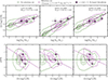 |
Fig. E.1. Top: The MZR for the ‘No SFR dependence’ case toy model with three different MZR parameters. We also plot our direct-Te metallicity estimates. Bottom: Specific star formation rate (sSFR) as a function of gas-phase metallicity. We show sSFR vs. gas-phase metallicity for our Hγ stellar mass binned stacks. The error bars on the sSFR are calculated using the 16th and 84th percentile in the stacks. The panels on the left are following the parameters by Curti et al. (2024), the middle panels follow the parameters by Heintz et al. (2023) and the panels on the right follow paramters by Sarkar et al. (2025) for Eq. 4. |
All Tables
Metallicity and SFR measurements in bins of stellar mass for the Hγ sample with 6.3 < z < 7.
Metallicity and SFR measurements in stellar mass bins for the Hβ (5.5 < z < 7) sample.
Gas-phase metallicity estimates in stellar mass bins for the Hβ (5.5 < z < 7) sample using R3 calibration.
All Figures
|
Fig. 1. Relation between UV magnitude and stellar mass for our Hβ sample (792 galaxies). The MUV and stellar masses were obtained through SED fitting using Prospector. With data from the ABELL2744 lensing field, we probed galaxies with MUV down to −16.6 mag. The UV luminosity increases with stellar mass, as was expected. |
| In the text | |
|
Fig. 2. Median stacked 1D rest-frame emission-line spectrum of the full sample of 792 [O III] emitters at z = 5.5–7. Each galaxy spectrum has been normalised by its ([O III]λ5008+2.98[O III]λ4960)/2 flux before stacking. The shaded green region shows the uncertainty estimated through bootstrap resampling. We highlight the wavelengths of Hδ, Hγ, [O III]λ4364, Hβ, [O III]λλ4960, 5008, and HeIλ5877. For visualisation, we normalised the stacked spectrum by the Hβ luminosity such that Hβ peaks at unity. |
| In the text | |
|
Fig. 3. Median stacked 1D rest-frame emission-line spectra of the Hγ sample (z = 6.3–7), in three stellar mass bins offset for visualisation purposes. The shaded region shows the uncertainty estimated through bootstrap resampling. In the right panel, we zoom into the wavelength range containing Hγ and [O III]λ4364. We fitted a complex of three Gaussians with the same standard deviation to obtain the fluxes of Hγ and [O III]λ4364. An additional Gaussian component was fitted to account for possible contamination by [Fe II]λ4360. |
| In the text | |
|
Fig. 4. R3 ratio as a function of stellar mass ratios for the entire dataset. Galaxies with S/N(Hβ) ≥ 3 are shown in blue and galaxies with S/N(Hβ) < 3 are shown in green with lower limits. Stars show measurements in stacked spectra. |
| In the text | |
|
Fig. 5. Relation between the gas-phase metallicity measured using the direct Te−method and the R3 ratio. We compare our estimates with several strong-line metallicity calibrations from literature. We show the calibration by Bian et al. (2018), which uses local analogues that occupy similar regions to z ∼ 2 star-forming galaxies on the BPT diagram, the calibration based on local galaxies with EW(Hβ) ≥ 200 derived by Nakajima et al. (2022), Hirschmann et al. (2023) calibration for z > 4 galaxies from the TNG100 simulation, and Sanders et al. (2024) and Chakraborty et al. (2025) calibrations for high-z galaxies between 2 < z < 10. |
| In the text | |
|
Fig. 6. Mass-metallicity relation from our stacked Hγ sample (purple stars, 6.3 ≤ z < 7). For the highest-mass bin in the Hβ sample, we also show the metallicity estimate from the higher-metallicity branch of the Sanders et al. (2024) R3-calibration curve (unfilled black star). The metallicity estimates and median stellar masses for both the samples are reported in Tables 1 and 2. The errors on the stellar mass were calculated using the 16th and 84th percentile values in the stack. While our measurements are from stellar-mass binned and stacked NIRCam grism spectra, similar to Li et al. (2025), measurements from Li et al. (2023) and He et al. (2024) were obtained using stacked spectra from NIRISS grism, measurements from Chakraborty et al. (2025), Chemerynska et al. (2024) and Pollock et al. (2025) are from individual galaxies, values from Curti et al. (2024) and Nakajima et al. (2023) are average metallicity measurements obtained from NIRSpec spectroscopy, and values from Faisst et al. (2025) were obtained from NIRSpec/IFU observations of high-mass main-sequence galaxies with [C II]158 μm observations from ALMA. |
| In the text | |
|
Fig. 7. Mass-metallicity relation inferred for our Hγ sample using the direct-Te method (purple stars), Chakraborty et al. (2025) R3-calibration (blue stars), Sanders et al. (2024) R3-calibration (magenta stars), and the Nakajima et al. (2022) R3-calibration for local galaxies with EW(Hβ) > 200 Å (green stars). We used metallicity estimates from the lower branch of the R3-calibrations. The use of strong-line methods leads to an artificial flattening of the observed relation. |
| In the text | |
|
Fig. 8. Mass-metallicity relation for the SPHINX20 (Katz et al. 2023) and FLARES simulation (Lovell et al. 2020; Vijayan et al. 2020), and the JAGUAR catalogue (Williams et al. 2018). We plot both the intrinsic MZR and the MZR after mimicking our selection cut. We also show the MZR from our stacked Hγ (purple stars) sample. The MZR slopes and normalisations are listed in Table B.1. |
| In the text | |
|
Fig. 9. Top: MZR for the three cases in our toy model. We also plot our direct-Te metallicity estimates. Bottom: Specific star formation rate (sSFR) as a function of gas-phase metallicity. We show sSFR vs. gas-phase metallicity for our Hγ stellar mass binned stacks. The error bars on the sSFR were calculated using the 16th and 84th percentile in the stacks. The top left and bottom left panels show Case 1 (‘normal FMR’). Our selection cut makes the MZR slope steeper. The top middle and bottom middle panels show Case 2 (‘no FMR’). Our selection cut does not affect the MZR slope. The top right and bottom middle panels show Case 3 (‘inverted FMR’). Our selection cut makes the MZR slope appear flatter. In all three cases, we find a negative correlation between sSFR and 12+log(O/H) upon implementing our selection cut. |
| In the text | |
|
Fig. C.1. [O III]λ5008 luminosities as a function of stellar mass for the SPHINX20 (Katz et al. 2023) and FLARES simulation (Lovell et al. 2020; Vijayan et al. 2020), the JAGUAR catalogue (Williams et al. 2018). We plot both, the intrinsic relation and the relation after mimicking our selection cut. We also show the L[O III]λ5008−log(M★/M⊙) relation for our stacked Hγ (purple stars) and Hβ (orange stars) sample. |
| In the text | |
|
Fig. E.1. Top: The MZR for the ‘No SFR dependence’ case toy model with three different MZR parameters. We also plot our direct-Te metallicity estimates. Bottom: Specific star formation rate (sSFR) as a function of gas-phase metallicity. We show sSFR vs. gas-phase metallicity for our Hγ stellar mass binned stacks. The error bars on the sSFR are calculated using the 16th and 84th percentile in the stacks. The panels on the left are following the parameters by Curti et al. (2024), the middle panels follow the parameters by Heintz et al. (2023) and the panels on the right follow paramters by Sarkar et al. (2025) for Eq. 4. |
| In the text | |
Current usage metrics show cumulative count of Article Views (full-text article views including HTML views, PDF and ePub downloads, according to the available data) and Abstracts Views on Vision4Press platform.
Data correspond to usage on the plateform after 2015. The current usage metrics is available 48-96 hours after online publication and is updated daily on week days.
Initial download of the metrics may take a while.