| Issue |
A&A
Volume 706, February 2026
|
|
|---|---|---|
| Article Number | A266 | |
| Number of page(s) | 17 | |
| Section | Astrophysical processes | |
| DOI | https://doi.org/10.1051/0004-6361/202556631 | |
| Published online | 13 February 2026 | |
XMM-Newton multi-year campaign on NGC 55 ULX-1
Resolving the wind and its variability with RGS
1
INAF – IASF Palermo Via U. La Malfa 153 I-90146 Palermo, Italy
2
Università degli Studi di Palermo, Dipartimento di Fisica e Chimica Via Archirafi 36 I-90123 Palermo, Italy
3
Center for Astrophysics – Harvard & Smithsonian Cambridge MA, USA
4
Department of Astronomy & Physics, Saint Mary’s University 923 Robie Street Halifax NS B3H 3C3, Canada
5
Université de Toulouse, CNRS, IRAP, 9 Avenue du colonel Roche BP 44346 F-31028 Toulouse Cedex 4, France
6
INAF – Istituto di Astrofisica Spaziale e Fisica Cosmica di Milano Via A. Corti 12 20133 Milano, Italy
7
Institute of Space Sciences (ICE), CSIC, Campus UAB Carrer de Can Magrans s/n E-08193 Barcelona, Spain
8
INAF – Osservatorio Astronomico di Cagliari, Localita Poggio dei Pini Strada 54 09012 Capoterra, Italy
9
Department of Physics, Centre for Extragalactic Astronomy, Durham University South Road Durham DH1 3LE, UK
10
INAF – Osservatorio Astronomico di Brera Via E. Bianchi 46 23807 Merate (LC), Italy
11
INAF – Osservatorio Astrofisico di Torino Strada Osservatorio 20 I-10025 Pino Torinese, Italy
12
Centre for Astrophysics Research, University of Hertfordshire College Lane Hatfield AL10 9AB, UK
★ Corresponding author: This email address is being protected from spambots. You need JavaScript enabled to view it.
Received:
28
July
2025
Accepted:
16
December
2025
Abstract
Context. Winds are an important ingredient in the evolution of X-ray binary (XRB) systems, particularly those at high accretion rates such as ultra-luminous X-ray sources (ULXs), because they may regulate the accretion of matter onto the compact object.
Aims. Our aim is to understand the properties of ULX winds and their link with the source spectral and temporal behaviour.
Methods. We performed high-resolution X-ray spectroscopy of the variable source NGC 55 ULX-1 to resolve emission and absorption lines as observed with XMM-Newton at different epochs. Optically thin plasma models were used to characterise the wind.
Results. We confirmed and thoroughly strengthened previous evidence of outflows in NGC 55 ULX-1. The presence of radiative recombination signatures and the ratios of the fluxes of the emission lines favours photoionisation balance and low to moderate densities, which confirm that the lines originate from classical XRB disc winds. An in-depth parameter space exploration shows line emission from a slowly moving, cool, and variable plasma perhaps associated with a thermal wind. Mildly relativistic Doppler shifts (about −0.15c) associated with the absorption lines confirm, at higher confidence, the presence of powerful radiatively driven winds.
Conclusions. The comparison between the results obtained at different epochs revealed that the wind responds to the variability of the underlying continuum. These variations may be used to understand the actual accretion regime and the nature of the source.
Key words: accretion / accretion disks / X-rays: binaries / X-rays: individuals: NGC 55 ULX-1
© The Authors 2026
 Open Access article, published by EDP Sciences, under the terms of the Creative Commons Attribution License (https://creativecommons.org/licenses/by/4.0), which permits unrestricted use, distribution, and reproduction in any medium, provided the original work is properly cited.
This article is published in open access under the Subscribe to Open model. This email address is being protected from spambots. You need JavaScript enabled to view it. to support open access publication.
1. Introduction
Ultra-luminous X-ray sources (ULXs) occupy the brighest end of the luminosity function of X-ray binaries (for recent reviews on ULXs, see King et al. 2023; Pinto & Walton 2023). Shining in the X-ray band (0.3−10 keV) above 1039 erg s−1, i.e. the Eddington limit for a stellar-mass black hole, they have been a matter of lively debate in the last two decades, particularly thanks to important discoveries enabled with the X-ray telescopes on board the XMM-Newton, Chandra, NUSTAR, and Swift satellites. We now know that most ULXs in the nearby Universe are powered by stellar-mass compact objects, such as neutron stars (NSs) and black holes (BHs), accreting above their Eddington limit, and they therefore represent the most extreme mass-transfer phase of interacting X-ray binaries (XRBs). This was particularly cemented after the discovery of coherent pulsations in a handful of nearby bright sources (dubbed PULXs; see e.g. Bachetti et al. 2014; Fürst et al. 2016; Israel et al. 2017).
High-quality broadband spectra of ULXs often peak in the X-ray band and show a peculiar curvature below 10 keV, which favoured a scenario of high mass transfer even before the discovery of the pulsations (see e.g. Gladstone et al. 2009; Bachetti et al. 2013; Walton et al. 2014). These spectra also revealed the presence of unresolved features in the soft X-ray band and, particularly, around 1 keV (see e.g. Soria et al. 2004; Stobbart et al. 2006; Middleton et al. 2015a) which were then unambiguously identified as a forest of emission and absorption lines via the high-resolution grating spectrometers on board XMM-Newton and Chandra (see e.g. Pinto et al. 2016; van den Eijnden et al. 2019; Kosec et al. 2021). These unveiled the long-sought winds driven by strong radiation pressure, which were the ultimate proof of supercritical accretion (see e.g. Ohsuga et al. 2005; Poutanen et al. 2007).
Ultra-luminous X-ray source winds have Doppler motions that reach velocities of about 0.2c; they have often been invoked as the engine powering the interstellar bubbles found around many ULXs (see e.g. Pakull et al. 2010; Gúrpide et al. 2022). Moreover, super-Eddington winds are expected to be equatorial and highly clumpy, and are likely able to scatter the hard X-ray photons coming from the innermost regions of the accretion disc, thereby influencing the way the ULX appears depending on the source view angle (see e.g. Middleton et al. 2015b; Kobayashi et al. 2018). For this reason, multi-epoch observations of variable and bright ULXs provide an ideal workbench to study the geometry and structure of super-Eddington winds, their influence on the source appearance, and the overall kinetic budget.
2. NGC 55 multi-year monitoring
NGC 55 ULX-1 is the brightest X-ray source in its host galaxy. At a distance of about 1.94 Mpc1, this source has a peak X-ray luminosity (0.3−10 keV) of about 4 × 1039 erg s−1 (see e.g. Gúrpide et al. 2021). The long-term Swift/XRT monitoring performed in 2013 showed substantial variability over a few weeks: a factor of 3−4 in the 0.3−10 keV band with the spectrum appearing harder when brighter, as already shown in many other ULXs, which has been ascribed either to having a clearer view of the inner accretion flow (i.e. viewing this through a less dense wind) when the flux is higher or to changes in the accretion rate through the disc (Pintore et al. 2015). On short timescales (∼100 s), Chandra and XMM-Newton light curves taken during the highest-flux epochs have shown sharp drops, during which the source exhibits softer spectra and significantly suppressed flux above ∼2 keV (Stobbart et al. 2006). This behaviour is more often seen in supersoft ULX sources (SSULs) and is likely due to wind clumps that temporarily obscure the innermost part of the disc (Urquhart & Soria 2016). For this reason, NGC 55 ULX-1 is thought to be at an inclination slightly lower than that of SSUL (e.g. Pinto et al. 2017, hereafter P17). Due to its flux and spectral variability, NGC 55 ULX-1 is an ideal target for studying the behaviour of the wind during different epochs and its role in the X-ray spectral appearance. In addition, its X-ray luminosity oscillates around 2 × 1039 erg s−1, which means that we can use it as a proxy for a compact object behaviour crossing the Eddington limit in the case the accretor is a stellar-mass BH, as indicated by recent results (Barra et al. 2022, hereafter B22).
2.1. Swift/XRT long-term monitoring
In order to study NGC 55 ULX-1 with deep (about 1 orbit) XMM-Newton observations in different flux regimes and to understand its long-term behaviour, we regularly monitored the source with the Swift XRT (Gehrels et al. 2004) from early 2020 to the end of 2023. The XRT light curve was retrieved via the web tool2 (Evans et al. 2009). Two long-term light curves were also extracted in the 2−10 keV and 0.3−2 keV bands to compute a hardness curve (hard/soft ratio; see Fig. 1). The band split was chosen at 2 keV because most variability is seen below this energy (see e.g. B22). Variability of up to an order of magnitude can be seen in the count rate on timescales of a few days.
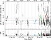 |
Fig. 1. Swift/XRT long-term light curve (top panel) and hardness ratio curve of NGC 55 ULX-1 (bottom panel). The hardness ratio is computed as the ratio of the counts in the 2−10 keV to 0.3−2 keV energy bands. The values for the four on-axis deep XMM-Newton observations are shown with horizontal lines and the times of the events with X markers followed by the corresponding ObsID. |
NGC 55 ULX-1 exhibits an absorbed 0.3−10 keV flux ranging from 1 × 10⁻¹² erg s−1 cm−2 during the dips to above 6 × 10⁻¹² erg s−1 cm−2 during flaring events (P17). A long archival (2010) observation with XMM-Newton caught NGC 55 ULX-1 at an intermediate flux corresponding to an XRT count rate of 0.07 c/s (converted via WEBPIMMS3 through an absorbed power-law model; e.g. Pintore et al. 2015). Our first new XMM-Newton visit observed the source during a low-flux period in November 2018, and we then tried to trigger two more observations during high-flux epochs, catching it at an intermediate flux in May 2020 (comparable to the archival 2010 data) and in the tail of a flaring period in December 2021.
2.2. First results of the XMM-Newton campaign
Our new observations enabled us to investigate the broadband properties of NGC 55 ULX-1 and to find strong evidence for a second transient ultra-luminous X-ray source (dubbed NGC 55 ULX-2) in the same galaxy. Regarding the new transient ULX, in Robba et al. (2022) we reported that the object is closer to the galactic centre and has a bolometric luminosity peak of about 3 × 1039 erg s−1 in multiple epochs. Its spectral shape and variability fits within the subclass of soft ultra-luminous X-ray sources (SULs). In B22, instead, we reported a detailed spectral modelling of ULX-1 with the high-statistics XMM-Newton/EPIC spectra. A double thermal model showed luminosity–temperature (L-T) trends in broad agreement with the L ∝ T4 relationship expected from a thin-disc model. However, small but significant deviations at the highest luminosities suggest that the disc structure is changing, for example due to an expansion or the contribution from the wind at accretion rates higher than the Eddington (ṀEdd) or even supercritical (∼ 2 − 3 ṀEdd), which in turn would indicate a stellar-mass black hole as the accretor.
In this paper we focus on the properties of ULX-1 winds by performing a detailed high-resolution X-ray spectroscopy with the reflection grating spectrometers (RGS) on board XMM-Newton. We include the archival data (2010) already shown in P17 in order to cross-check and validate our results. The rest of the manuscript is organised as follows. We report the XMM-Newton data reduction in Sect. 3 and the spectral modelling in Sect. 4. We discuss our results in Sect. 5 and provide our conclusions in Sect. 6. All uncertainties are given at the 1σ (68% level).
3. Data reduction
For this work we used the four on-axis deep XMM-Newton observations of NGC 55 ULX-1. These enabled us to obtain individual high-resolution RGS spectra along with the high signal-to-noise EPIC spectra, which are necessary to find and identify wind features, and track down any changes at different epochs. The observation IDs are 065505(0101) (05/2010), 082457(0101) (11/2018), 086481(0101) (05/2020), and 088396(0101) (12/2021). To avoid redundancy, we do not show all the details regarding the EPIC data reduction since it was already reported in B22. Briefly, raw data were retrieved from the XMM-Newton Science Archive (XSA)4 and reduced with the Science Analysis System (SAS) version 22.1.05 with recent calibration files (February 2025). The EPIC MOS and pn data were processed with the EPPROC and EMPROC tasks according to the standard procedures regarding patterns and solar flare removal. The clean exposure times were identical to those reported in B22. The source spectra were extracted using a circular region of 20″ radius (to keep background contamination low) centred on the X-ray position estimated with Chandra (RA: 00h 15m 28.89s Dec: −39° 13′ 18.8″; Gladstone et al. 2009) while the background was selected from a larger circular region a few arcminutes away from the source and from the copper ring in the same chip. The response matrices and effective area files were extracted with the RMFGEN and ARFGEN tasks. We also stacked the EPIC-pn, MOS 1, and MOS 2 spectra from the four observations using EPICSPECCOMBINE in order to obtain three time-averaged spectra with high signal-to-noise ratio for the SUL regime of NGC 55 ULX-1 (see Fig. 2).
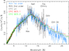 |
Fig. 2. XMM-Newton combined spectra of ULX-1 obtained by stacking those from the four deep on-axis observations: RGS first-order (light blue) and second-order (black), EPIC-pn (grey), MOS 1 (red), and MOS 2 (green). |
The RGS data reduction was performed with the RGSPROC, which also extracts spectra and response and area files. We extracted the first- and second-order RGS spectra in a cross-dispersion region of 0.8′ width, centred on the source coordinates and the background spectra by selecting photons beyond the 98% of the source point spread function. The background regions do not overlap with bright sources. We filtered out periods affected by contamination from solar flares by selecting background-quiescent intervals in the light curves of the RGS 1, 2 CCD 9 (i.e. ≳1.7 keV) with a standard count rate below 0.2 c/s. As is typically found, solar flares affected the RGS data to a much lower extent than the EPIC data. The total clean exposure times for each RGS spectrometer are 120, 135, 129, and 122 ks for ObsID 0655, 0824, 0864, and 0883, respectively. The four observations yield RGS 1+2 first-order spectra with a total of 5773, 4545, 7853, and 5465 source-net counts, respectively. Typically, ≳5000 counts are necessary to detect the strongest lines (Kosec et al. 2021).
We used the RGSCOMBINE task to produce a combined spectrum for the first order, which yields a total of 23 636 counts and an exposure of 506 ks, which is one of the ten deepest ULX RGS spectra and the second-deepest SUL spectrum after that of NGC 5408 ULX-1 (Pinto et al. 2016; Kosec et al. 2021; Pinto & Walton 2023). Finally, we also combined all the second-order RGS 1 and 2 spectra obtaining a 7536-count spectrum with good statistics, which provides the clearest view around 1 keV (or 12 Å) with a resolving power λ/Δλ > 300 and increasing at lower energies; see Figs. 2 and 3.
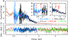 |
Fig. 3. XMM-Newton time-averaged (on-axis) spectra and continuum model. The labels are the same as in Fig. 2. The EPIC data were ignored in the range 0.5−1.8 keV in order to fully employ the high spectral resolution of RGS and decrease degeneracy between models of line emission and absorption. |
We note that spectral stacking is necessary to speed up computation, particularly to run Monte Carlo (MC) simulations that are suitable for estimating the signification of the line detection. This already takes about a month for an accurate scanning of spectral lines in a statistical sample of simulated spectra (see Sect. 4.3 and the dedicated discussion in Pinto & Walton 2023).
We also had a quick look at the data from the Optical Monitor (OM) on board XMM-Newton to search for an optical/UV counterpart of ULX-1. The source was undetected in the images provided by all filters (V, UVW1, UM2, and UVW2) and by stacking those from the same filters. This was expected given its very low flux in observations with Hubble Space Telescope (HST magnitude ≳23; Gladstone et al. 2013; Zhou et al. 2023).
4. Spectral modelling
The spectra were modelled with the SPEX fitting package 3.08.01 (Kaastra et al. 1996), which has a full suite of line-emitting/absorbing optically thin plasma. The spectra were grouped according to the optimal binning directly in SPEX, which provides at least one count per bin and a bin size ≥1/3 of the spectral resolution, and fit by minimising the C-statistics (Cash 1979; Kaastra 2017). All the emission components were corrected for absorption from the circumstellar and interstellar medium with the hot model (freezing the gas temperature to 10−6 keV, which provides a neutral gas in SPEX). To limit the computation time, we adopted the recommended solar abundances of Lodders & Palme (2009), which are the default in SPEX, for all emitting and absorbing plasma components. This is generally a good approximation, although it might have an impact on the detection of the winds given that their abundances may differ from the solar pattern as recently shown in Holmberg II (UL)X-1 (Barra et al. 2024). Each model is fitted simultaneously to the EPIC MOS 1, 2/pn and RGS first- and second-order spectra with a free multiplicative constant that accounts for the typical 1−5% cross-calibration uncertainties.
Both the combined spectra and those of the individual observations were analysed with the following scheme: continuum modelling, Gaussian line scan, physical model scan, and best-fit physical model. We first focused on the high-statistics time-averaged stacked spectrum in order to identify the main features and/or lines in the RGS spectrum and search for evidence of outflows. Afterwards, we performed an analysis of the individual observations to search for any variability in the lines and outflow parameters (see Sect. 4.2).
4.1. Time-averaged spectrum
The combined EPIC MOS 1, 2/pn and RGS first and second spectra are shown in Fig. 2. By visual inspection it is easy to spot the well-known O VIII H-like emission line around 19 Å, the He-like O VII emission feature near 22 Å, and the 23 Å oxygen K-edge, which were previously found in the archival data and in many more ULXs (P17, Kosec et al. 2021). Due to its higher resolution, the second-order spectrum resolves the feature around 1 keV in what looks like a sharp drop below 11 Å. This is similar to that observed at lower resolution in SSUL spectra and previously interpreted as an edge due to photon absorption in the wind (see e.g. Urquhart & Soria 2016; Pinto et al. 2021).
4.1.1. Continuum modelling and spectral energy distribution
The RGS and EPIC time-averaged spectra were simultaneously fitted. In order to fully employ the high resolution of RGS and decrease the degeneracy between models, we ignored the EPIC data within 0.5−1.8 keV where the RGS source spectrum is well above the background. A two-component emission model was adopted following P17, i.e. a cool 0.16 ± 0.01 keV blackbody (bb) and a warmer 0.70 ± 0.01 keV bb modified by coherent Compton scattering (i.e. mbb) for the broader–harder component produced by the hotter super-Eddington inner disc. The best-fit column density is (2.5 ± 0.1) × 1021 cm−2. This time-averaged value was also adopted later for the fit of the individual observations as it is not expected to vary significantly (P17, B22). The 0.3−10 keV (unabsorbed) luminosities of the cool and warm thermal components are around 9.4 × 1038 erg s−1 and 5.6 × 1038 erg s−1 for a total of 1.5 × 1039 erg s−1, while the total observed flux is around 1.5 × 10⁻¹² erg s−1 cm−2. The best-fit continuum model is shown in Fig. 3. Sharp narrow residuals can be seen along with the drop above 1 keV mentioned above.
In Sect. 4.1.3 we show the application of photoionisation (and collisional) models. For the computation of photoionisation equilibrium, a broadband spectral energy distribution (SED) is necessary. Following the Pinto et al. (2021) approach on a similar source (soft or supersoft NGC 247 ULX-1), we extrapolated the (unabsorbed) best-fit double thermal model down to 10−4 keV and up to 102 keV, for a total bolometric luminosity of 1.7 × 1039 erg s−1. Most of the flux for this type of object is produced in the 0.3−10 keV range, which results in low systematic uncertainties due to the broadband extrapolation (see e.g. Pinto et al. 2020a).
4.1.2. Gaussian line scan
In order to search for narrow spectral lines, we performed a Gaussian line scan consisting of a fit with a moving Gaussian line with the method outlined in (Pinto et al. 2016, P17). In addition to the bb+mbb continuum model, we added a Gaussian with the centroid shifting from 0.5 to 7 keV (above which EPIC spectra are background-dominated), exploring the presence of lines also in the EPIC spectra, particularly above 2−3 keV where the CCD spectral resolution progressively increases. We used a logarithmic grid with 500 (resp. 3000) steps for the adopted velocity dispersion (σV = FWHM/2.355) of 5000 (resp. 100) km/s. This was used to mediate between the resolving power needed for a given line width and the computation time, and to search for lines from plasma going from thermal (e.g. broadening around 100 km/s) to the more extreme outflows seen in other ULXs, particularly for a (S)SUL regime similar to NGC 55 ULX-1 (e.g. NGC 247 ULX-1, Pinto et al. 2021).
The single-trial significance was computed as the square root of the ΔC-stat improvement with respect to the continuum, and was then multiplied by the sign of the Gaussian normalisation to distinguish between emission-like and absorption-like features. The line scan gets rid of some noise in the plot and improves visualisation of possible spectral features including those in emission near the 1s–2p transitions of O VII-VIII and Ne IX-X. These were previously found in the scan of the archival ObsID 0655050101 (P17) and in other ULXs (e.g. NGC 1313 ULX-1 and NGC 247 ULX-1; Pinto et al. 2016, 2021), although some clearly show evidence of Doppler shifts (see Fig. 4). Further absorption-like features were found between 0.7 and 0.8 keV and above 1 keV, just as in the archival ObsID 0655050101 (P17). Additional negative residuals can be seen between 3 and 4 keV in the EPIC spectra, away from any significant instrumental features in the mirror response, likely from blueshifted Si-S lines.
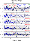 |
Fig. 4. Gaussian line scan of the XMM-Newton time-averaged spectrum (top panel) and spectra of the individual observations. Labelled are the energy centroids of some of the most common X-ray spectral lines; Fe K refers to the Fe I fluorescence and the Fe XXV resonant lines. The grey vertical line indicates the separation between RGS and EPIC. The grey-shaded areas indicate the 3σ single-trial significance. |
We attempted a quick modelling of the dominant emission lines with simple Gaussian profiles since they appear very narrow and close to their laboratory wavelengths (see Fig. 5). The centroids of the weak Lyman α (Lyα) lines from Mg XII and Ne X and the He-like triplets from Mg XI and Ne IX are consistent with their rest values. The Fe XVII lines, which are often signatures of collisional plasma, are not significantly detected. The lines from cooler plasma (e.g. O VIII Lyα and the O VII triplet) are blueshifted by about −1900 ± 200 km/s, as already found in P17, hinting at a slow outflow. Evidence of radiative recombination continua (RRCs), another signature of photoionisation, is shown by weak lines in proximity of the wavelengths expected for the abundant, recombining ions (O VII and N VI-VII). In particular, the presence of a N VII RRC is suggested by the presence of a rather strong line at 18.5−18.6 Å, which is difficult to explain only with O VIIβ line emission given that the measured flux is comparable to that of the O VIIα resonant line at 21.6 Å. The profile of these emission lines is not fully resolved due to their width being less than 1000 km/s. Tighter constraints were obtained by fitting multiple lines with a physical model (see Sect. 4.1.3). The relative ratios of He-like lines can be used to retrieve useful information on the plasma state, as we discuss in Sect. 5.
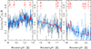 |
Fig. 5. XMM-Newton RGS time-averaged spectrum (order 1 in blue, order 2 in black) and Gaussian emission lines, zoomed in on the Mg-Ne K, Fe L, and O K edges. We note the weakness of the Fe lines, the stronger O VII forbidden line, and the tentative RRC profiles (with hints of photoionisation). |
4.1.3. Physical model scan
In order to identify the nature of the spectral features and correctly estimate any Doppler shift, we performed a modelling through the aid of optically thin thermal plasma. We tested emission and absorption models of plasma in collisional ionisation (CIE) or photoionisation (PIE) equilibrium, but focused mainly on the latter given the nature of the source and the variability of the X-ray spectral lines seen in other ULXs (see e.g. Pinto et al. 2020b, 2021; for more details, see Sect. 4.2). As we potentially expect large Doppler shifts of the plasma, to find the global best spectral fit we performed a deep exploration of the parameter space for the two most relevant parameters: the Doppler shift or velocity projected along the line of sight (vLOS) and the plasma state parameter (the temperature, kT, for CIE and the ionisation parameter ξ = Lion/nHR2 for PIE, where Lion is the ionising luminosity, nH the volume density, and R the distance of the plasma from the ionising source).
CIE – line emission. In the case of line-emitting CIE plasma similar to a collimated outflow or a SS433-like jet (Marshall et al. 2002), we adopted the cie component in SPEX, which calculates the emission spectrum of a plasma in collisional equilibrium. The cie component was multiplied by the redshift component reds in SPEX to account for Doppler shifts. We then computed (vLOS, kT) cie model grids and left the normalisation (or emission measure) free to vary. We adopted a logarithmic grid of temperatures between 0.1 and 5 keV (50 points), and a linear grid of line-of-sight velocities, vLOS, between −0.3c (blueshifted jet) and +0.3c (redshifted jet). We tested a velocity dispersion vσ of 100, 1000, 5000, and 10 000 km/s with LOS velocity steps of 300, 700, 1000, and 1500 km/s, respectively, to speed up the computation, as was done for the Gaussian line scan (see Sect. 4.1.2 and Kosec et al. 2018). The kT range was chosen below 5 keV because any hotter component would produce dominant lines above 5 keV, i.e. in the region where the EPIC BKG becomes important and out of the RGS reach. Moreover, the RGS energy range is too short to distinguish weak lines emitted by plasma with kT of a few keV or higher (see e.g. Lepore et al. 2025).
Given the limited number of counts for individual lines and the integration time and the variability of the line centroid, which could smear out the triplets when stacking all the spectra, we do not expect to obtain strong constraints on the relative ratios of the He-like triplets, for example those of O VII and Ne IX. This implies loose constraints on the plasma volume (or number) density, whose fitting may result in an unnecessary increase in the computation time. We therefore chose not to fit the volume density and adopted nH = 1010 cm−3, which is a lower limit found for NGC 1313 ULX-1 (Pinto et al. 2020b) and agrees with the measured O VII line ratios (see Sect. 5.1). This might only slightly affect the overall flux and column density of the line-emission component.
A loop is computed throughout these model grids, and is shown as a contour plot for vσ = 100 km/s in Fig. 6 (top panel). Multiple solutions appear with temperatures around 1−2 keV and different vLOS (a few thousand km/s, very similar to NGC 247 ULX-1, −0.08c and −0.2c previously reported in P17 for ObsID 0655050101). The overall ΔC-stat is well above 30, which according to previous work already indicates a highly significant detection, although a strong degeneracy seems to be present for this particular model.
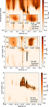 |
Fig. 6. XMM-Newton time-averaged grids of physical models. From top to bottom: CIE (cie model) emission, PIE (pion) emission, and (xabs) absorption. The black contours refer to significance levels from 3 to 5σ with steps of 0.5σ estimated with MC simulations (Sect. 4.3). |
We did not test the CIE absorption plasma as it is not expected to dominate the absorption measure distribution, particularly in the presence of a strong X-ray radiation source (the ULX itself). Moreover, with the present spectral quality and signal-to-noise ratio, it would be challenging to distinguish CIE from PIE absorption models because they both mainly produce absorption lines related to the electron transitions from the resonant levels.
PIE – line emission. As mentioned above, the input SED for the photoionisation balance computation was extrapolated from the best-fit continuum model (see Appendix A.1 and Fig. A.1). The pion model in SPEX can be used to produce spectra of PIE plasma both in emission and absorption, depending on the adopted values for the solid angle Ω/4π and the covering fraction fcov, which vary between 0 and 1 by definition. In the case of emission-line spectra, we fixed Ω/4π = 1 and fcov = 0 to speed up the computation. We scanned the time-averaged EPIC+RGS spectra with the grids of pion models (in addition to the continuum model) with the same multi-dimensional routine used for the cie model, and a similar parameter space (actually identical for the Doppler shift). We adopted a logarithmic grid of ionisation parameters (log ξ [erg/s cm] between 0 and 6 with 0.1 steps). The only free parameter for pion is the column density, NH. As previously done for the cie grids, we adopted nH = 1010 cm−3 for the pion model grids. Unlike the cie grids, the pion grids show a clear absolute maximum with velocity −0.08c, i.e. an outflow, and a significantly higher ΔC-stat of 42 (see Fig. 6, middle panel). Further local minima were found at outflow velocities slightly above 0.1c and close to the rest frame, likely pointing towards a multi-phase or variable plasma, as suggested in P17, or a possible degeneracy between different solutions.
The CIE and PIE solutions at low temperature (kTe ≲ 0.2 keV or log ξ ∼ 1) and close to the rest frame (|vLOS|≲0.01c) are primarily responsible for fitting the O VII-VIII (and weaker Ne IX-X) features close to their laboratory wavelengths while those with intermediate temperature and velocity (−0.08c) describe the jump around 1 keV (as previously suggested in P17, albeit with greater significance in the combined data).
PIE – line absorption. For a fast execution of the parameter space exploration through grids of photoionised absorbing plasma (which is crucial for expensive MC simulations), we used the fast xabs model in SPEX. This adopts the ionisation balance pre-calculated through the SPEX task xabsinput once the SED is provided in input. The ionisation balance files used by xabs include the conversion of the ionisation parameter to the temperature and the ionic fraction for every element at a given value of log ξ. The grid of photoionised xabs models was calculated and fitted in the same way as the pion models, but assuming line-of-sight velocities, vLOS, ranging between −0.3c and zero (i.e. only rest-frame or outflowing plasmas in absorption because we do not expect extreme inflows). The xabs results are shown in Fig. 6 (bottom panel). Aside from some degeneracy between multiple solutions (likely driven by spectral stacking), it is obvious that the absorbing plasma flows out with a relativistic speed of −0.15c or higher, as found for the archival observation in P17. The very large ΔC-stat, well above 50, suggests a very high confidence level, most likely above 5σ (see below).
Given the particularly large improvement in the spectral fits and the presence of degeneracy due to the stacking process, we performed the final fits (with the addition of both emission and absorption components) only on the spectra of the individual observations (see below). Moreover, the multiple solutions are a characteristic of the combined spectrum. In the individual spectra only one solution is detected (if detection actually occurs; see Sect. 4.2). Given that a meaningful non-degenerate modelling aimed at comparing variability over time can be performed only on individual observations, we refrained from the test of more complicated emission models for the combined spectrum.
4.2. Individual observations
For individual observations, we repeated the several steps performed for the time-averaged spectrum. One main difference is that we do not include the second-order spectra of individual observations; their low statistics would result in an unnecessary increase in computing time. Our steps were the following:
-
Estimation of the continuum with the double thermal model, as done in Sect. 4.1.1. The spectra of individual observations are shown in Fig. A.2.
-
Performance of a Gaussian line scan for the individual spectra following the same approach as in Sect. 4.1.2. The results of the scan are shown in the lower panels of Fig. 4.
-
Multi-dimensional scanning of the spectra with different physical models (emission by collisional or photoionised plasmas and absorption by a photoionised plasma) following the same routine used in Sect. 4.1.3. The results of the CIE and PIE scans are shown in Fig. A.3. The black contours refer to the confidence level estimated via the MC simulations described in the following section. Diagnostic checks for secondary peaks, alternative solutions, and degeneracy were performed adopting the spectra from ObsID 0655050101 (see Appendix A.2 and Fig. A.4).
-
For the individual observations, we also produced plots for the best-fit continuum+wind model. Here, in addition to the double thermal continuum, we also added a combination of emitting (pion) and absorbing (xabs) photoionised plasma components (see Fig. A.5 and Table 1). In Appendix A.4 and Fig. A.7, we show the zoomed-in image of the RGS spectra highlighting the contributions of the main model components.
Table 1.Best-fit plasma parameters in each EPIC+RGS spectral fit.
-
As a diagnostic check, we substituted the xabs with the more accurate pion model in absorption (assuming Ω/4π = 0 and fcov = 1) and refitted the spectra starting from the best fit obtained with xabs (see Table 1). No significant change was observed and the uncertainties did not decrease with pion, for which we preferred to keep the results obtained with xabs to be consistent with the simulations performed.
4.3. Monte Carlo simulations and detection significance
The significance of the line detection was obtained by running identical searches in the same parameter space onto a large number of simulated featureless spectra. Following the code developed in Pinto et al. (2020b), we performed MC simulations of a physical model scan (PIE/xabs) onto 16 000 spectra that were simulated adopting the best-fit continuum model of the RGS+EPIC ObsID 0655050101. The results are shown in Fig. A.6. A histogram of ΔC-stat occurrences was produced to estimate the significance of the detection in real data. Given the stability of the histogram slope (−0.26) above about 5000 simulated spectra (as already noted in Pinto et al. 2021) a forecast was made for 1.5 × 10⁵ and 1.7 × 10⁶ simulations to enhance the significance sensitivity up to 4.5 and 5.0σ. The other observations have comparable exposure times, fluxes, and number of counts, which suggests that the results for ObsID 0655050101 can be extended to the others. In summary, the detections in the data that refer to ΔC-stat improvements above 22, 29, and 36 with respect to the continuum-only model correspond to confidence levels above 3, 4, and 5σ, respectively. The confidence levels can be seen as black contours in Fig. A.3. This exercise was repeated for the time-averaged spectrum (to quantify the significance of the detections in Fig. 6) for five thousand simulations. The histogram of the ΔC-stat occurrences has a comparable slope (about −0.25) and agrees with that from the MC simulations performed for NGC 247 ULX-1 and similar cases (e.g. Pinto et al. 2021; Kosec et al. 2021; Gu et al. 2022).
Final spectral fits were performed for the time-averaged and individual spectra. We tested two combinations of optically thin plasmas: a hybrid one with emitting CIE and absorbing PIE (cie + xabs) and a purely photoionised emitting plus absorbing (pion + xabs) plasma. The properties of the xabs did not change within the uncertainties given the narrow width of the lines. For the same reason, ΔC did not decrease significantly while fitting multiple components (they are not mutually dependent; see also the discussion in Pinto et al. 2021). In Table 1 we report the best-fit values, the spectral improvement, and the estimated significance of each component derived using the MC simulations. We also quote the bolometric luminosities once they were corrected for absorption from the xabs component. In addition, we also report the spectral hardness computed as the ratio of the two luminosities computed in the 2−10 keV and 0.3−2 keV energy bands (estimated with the continuum model fits). Finally, the root mean square estimated as the square root of the excess variance in the 0.3−10 keV light curves shown in B22 is also reported in the same table.
5. Discussion
In this section we address the nature of the optically thin plasma components and place some constraints on the nature of the accretor and its energetic feedback on the surrounding medium.
5.1. The nature of the line emitting plasma
The model grids showed multiple solutions when we adopted CIE plasma and low velocity dispersion (see Fig. 6), while a better fit was obtained with a very large broadening (vσ ∼ 7000 km/s; see Table 1). This means that the cie struggles to describe all features and that some solutions are degenerate.
The G − R line ratios, measured for the relevant He-like triplets such as those of O VII and Ne IX, may be useful to place constraints on the plasma density and temperature (see e.g. Porquet & Dubau 2000). The time-average RGS spectrum provides by far the best statistics and allows Gaussian modelling of the individual lines (see Figs. 2 and 5). Using the partly resolved O VII triplet (resonant r, intercombination i and forbidden f lines at 21.6, 21.8, and 22.1 Å, respectively), we obtain two lower limits R = f/i > 1.2 (at 68%, with the most probable value of around 4) and G = (f + i)/r > 1.2 (at 68%, with the most probable value of 4.6). We used the SPEX pion code to compute the R and G ratios for the O VII triplet as functions of the electronic density, ne, and the electronic temperature, T, respectively. As broadband SED we adopted the best-fit continuum model for the time-averaged spectrum. In output, through the ascdump command, pion provides the relationship between the ionisation parameter and the temperature, and much more information including the fluxes of the lines. We performed the computation through a grid of log ξ between 0 and 4.0 with 0.2 steps, and ne from 108 to 1014 cm−3 with a logarithmic step of 10. We also adopted a column density NH = 1022 cm−2 and vσ = 250 km/s, which agree with the best-fit values. The curves are plotted in Fig. 7. The comparison of such curves with the data measurements implies, through the G ratio, a temperature kT ≲ 105 K (consistent with the pion best-fit results; see also Fig. A.1). The R ratio instead yields a number density of around 7 × 1010 cm−3 (or an upper limit of 1011 cm−3). This suggests that we are looking at a photoionised plasma with a slightly lower density than that seen in Eddington-limited Galactic XRB winds or accretion disc coronae (see e.g. Psaradaki et al. 2018; Neilsen & Degenaar 2023 and references therein). The RGS resolution at 13 Å and signal-to-noise ratio are too low to place significant constraints on the Ne IX triplet.
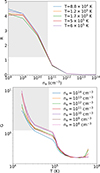 |
Fig. 7. O VII He-like triplet R (top) and G (bottom) ratio curves calculated from the time-averaged SED. The grey-shaded areas indicate the regions compatible with the results from the combined spectrum and the upper limits on the temperature and the density (see Sect. 5). |
From the definition of the ionisation parameter we can resolve for the density in order to obtain a constraint on the radius, i.e. the distance of the photoionised line-emitting plasma from the inner portion of the accretion disc,  . Assuming the upper limit of the density mentioned above and the pion best-fit parameters determined in the time-averaged spectrum (see Table 1), we obtained a lower limit on the distance R ≳ 7.3 × 1012 cm ∼0.5 AU (or 5 × 10⁶ RG for a 10 M⊙ black hole). This is similar to what was obtained for NGC 1313 ULX-1 (Pinto et al. 2020b). The semi-major axis of the orbits for similar systems, such as SS 433 and NGC 7793 P13, is of the order of 0.4 − 0.8 AU (Bowler 2011; Fürst et al. 2018, the Roche lobe would be even smaller), which would indicate a location further out than the outermost part of the accretion disc; this value is expected from an equatorial thermal wind. The entire binary might be engulfed in an optically thin line-emission envelope with a large solid angle, just as could occur in SS 433 (Waisberg et al. 2019). This slower outflow component might be associated with the broad Hα, consistent with emission from a hot disc wind (600 km/s, Zhou et al. 2023).
5.2. A multi-phase outflow
The presence of plasmas moving at about ±1000 km/s and −0.1c (in emission) and around −0.15c (in absorption) points towards a stratified, likely multi-phase, outflow. We also note that the pion modelling of the combined spectrum favours a fast −0.08c outflow with an ionisation parameter higher (log ξ = 2.5) than the individual fits, due to a secondary solution that is present in all scans and is evident once all data are taken into account (see Table 1). The fastest components provide evidence for mildly relativistic matter driven by the strong radiation pressure. Their velocities and temperatures agree with the predictions from the theoretical simulations of super-Eddington accretion (see e.g. Ohsuga et al. 2005; Takeuchi et al. 2013). Such high Doppler velocities with a corresponding low-velocity broadening are also in line with the recent results obtained with the high-resolution Fe K spectra of highly accreting supermassive black holes taken with the XRISM/Resolve microcalorimeter (see e.g. Xu et al. 2025; Xrism Collaboration 2025). The low-velocity low-temperature plasma responsible for the narrow O VII-VIII emission lines is most likely a result of thermal pressure and ionisation of the outer regions of the disc (also known as thermal winds; see e.g. Pinto & Walton 2023). Using the ionisation balance (kTe − log ξ curves) computed with pion, we estimated a temperature above 104 K and a ratio of about 10 between the radiation pressure (F/c) and the thermal pressure (nHkT), which is given by Ξ = F/nHckT = 19 222 ξ/T, with F = L/4πR2 (Krolik et al. 1981) (see Fig. A.1). These values agree with the expectation of the theory of thermal winds (see e.g. Middleton et al. 2022).
A comparison is performed between the plasma properties to address its thermal stability, in particular, through the S curve. The S curve is described as the relationship between the state parameter (kT or ξ) and the radiation-to-thermal pressure ratio Ξ (see Fig. A.1). Neither the pion nor the xabs best-fit ξ values are found in correspondence with negative slopes or unstable branches with the exception of the absorbing plasma (vLOS = −0.05c and log ξ = 1.26) exhibited in the highest-flux observation (0883960101) and, at a lower significance, in the first intermediate-flux observation. This would indicate a sporadic event or even a failed wind (e.g. Petrucci et al. 2021; Miller et al. 2025). The presence of an instability branch between log ξ = 1.1 − 1.2 confirms that the slow–cool and fast–hot plasma components are not in thermal balance with each other and that the outflow is multi-phase. In other words, these two components (line-emitting and absorption-line) do not share the same origin: the slow one was produced by the outer disc photosphere and the fast one by the inner super-Eddington accretion disc. Alternatively, the former might have been from the inner disc and then slowed and cooled down to the lower branch due to other physical phenomena.
The last observation also shows a tentative secondary solution with a ∼0.25c redshift. It corresponds to the pion attempting a fit of a feature at 0.62 keV (which could also be explained with O VII blueshifted by −0.08c) and leftovers residuals in the complex oxygen K edge at 0.5 keV, which is mainly affected by the cold ISM (and the background). The difficulty to explain such a strong redshift along with the location of the features lead us to believe that it is most likely a spurious detection. We also note that the primary solution at −0.140c is pegged at its lower bound for both the pion and the cie due to the weakness of lower ionisation lines and sensitivity at lower temperatures.
5.3. Comparison with other ULXs: A ubiquitous 1 keV line
As mentioned in Sect. 1, high-count CCD spectra regularly show unresolved spectral residuals around 1 keV. Among the several proposed scenarios, the one with super-Eddington relativistic winds was a tantalising solution (see e.g. Middleton et al. 2014, 2015a). In Pinto et al. (2016), the features were resolved for the first time in two ULXs. Simultaneous EPIC+RGS fits indicated that the RGS-detected winds were responsible for most of the EPIC residuals. In soft or supersoft ULX spectra the feature around 1 keV looks like an absorption edge; this is also observed in extragalactic XRBs with LX ∼ 1039 erg/s (see e.g. Urquhart & Soria 2016; Earnshaw & Roberts 2017). This would point to evidence of absorption by winds. The results we obtained for SUL NGC 55 ULX-1 and those recently shown for SUL-SSUL NGC 247 ULX-1 show that the feature is actually a combination of high-velocity plasma (|v|≳0.15c) in absorption and low-velocity plasma (|v|< 0.1c) in emission primarily Ne K and Fe L ions with contribution from the O VIII edge whose laboratory energy is 0.87 keV, which is shifted above 1 keV for |vLOS|≳0.15c). The line-emitting plasma exhibits a 0.3−10 keV luminosity in the range (0.4 − 1.2)×1038 erg/s, which is of the same order of magnitude as that measured in the RGS spectra of other ULXs although clearly around a factor of about 2 lower than in NGC 1313 ULX-1, NGC 5408 ULX-1, and NGC 247 ULX-1 (Pinto et al. 2016, 2020b, 2021). This could be the result of a higher Eddington ratio, and therefore stronger radiation pressure in the brighter sources, as noted in a small sample of highly accreting supermassive black holes (Xu et al. 2023).
5.4. The nature of the accretor
The highest significance of ultra-fast winds in the time-averaged spectrum implies a long-term sustained radiation pressure, and therefore an intrinsic luminosity that is regularly above the critical value, i.e. Lcr ∼ 9/4LEdd. Moreover, once absorption by the photoionised plasma (xabs) is taken into account, the corrected bolometric luminosity appears to be above 2.5 × 1039 erg/s (i.e. 50% higher). In B22, it was suggested that the deviations in the L − T diagram could be interpreted as an increasing contribution of the winds to the soft (< 2 keV) X-ray emission at LBOL ≳ Lcr which would imply a small compact object mass (5 M⊙). If we account for the correction due to photoionised absorption we predict a black hole with a typical mass (7.5 M⊙). If we instead assume that the deviations occur at LBOL ∼ LEdd, a heavier (17 M⊙) black hole would result, which agrees with arguments related to mass inflow and outflow rates (Fiacconi et al. 2017).
5.5. The wind temporal evolution
In Figs. 8, 9, and 10 we compare the best-fit values of the main parameters of the emitting and absorbing plasmas obtained for individual observations and (in red) for the time-averaged spectrum. We recall that two of the four observations (ObsID 065505 and 086481) occurred at similar luminosities, whereas the other two occurred during low-flux and flaring periods. The two equi-luminosity observations that occurred at the most common flux regimes of NGC 55 ULX-1 exhibit consistent wind properties with a dominant low-velocity emitting plasma and a mildly relativistic outflow (|vLOS|≳0.15c). The luminosity corrections are comparable and amount to 60−70%. The RMS are also consistent between these two observations (12−15%).
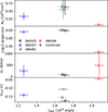 |
Fig. 8. Summary plot for the results relative to the xabs (photoionised absorber) model. The grey circles refer to the combined spectrum. |
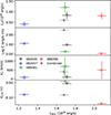 |
Fig. 9. Summary plot for the results relative to the pion (photoionised emitter) model. The grey circles refer to the combined spectrum. |
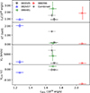 |
Fig. 10. Summary plot for the results relative to the cie (collisionally ionised emitter) model. The grey circles refer to the combined spectrum. |
The low-flux observation (ObsID 082457) shows similar wind properties for the absorber, indicating that the source is still in a super-Eddington regime. The spectra hardness, HR, is broadly constant between the different observations, indicating a similar state. However, the lower RMS and luminosity correction suggest that the source is intrinsically fainter during ObsID 082457, which is confirmed by the lower significance and two times fainter line-emitting component (see Table 1).
The highest-flux observation (ObsID 088396) caught the tail of a major flare. At the peak of the flare the observed flux was two times higher than the average level; see Fig. 1. ObsID 088396 is characterised by a moderate RMS (8%) and luminosity correction, indicating that some obscuration might still be present. Here, the fastest (−0.1c) absorbing component seen in the other observations appears clearly weakened, while there is a potential 3σ detection of an emerging component with a lower velocity (vLOS = −0.05c) and a lower ionisation parameter (log ξ = 1.3). This situation is remarkably similar to what was observed during the high-flux regime of NGC 1313 ULX-1, which was interpreted as being due to the extension of the launching radius or spherisation radius, defined as  with Rin = 6 RG, at increasingly higher super-Eddington rates (Pinto et al. 2020b). The fastest component might have weakened due to an increase of its ionisation parameter (which is proportional to the luminosity since ξ = Lion/nHR2) similarly to disappearing winds in highly accreting supermassive black holes (see e.g. Pinto et al. 2018). An intrinsically higher luminosity might be the reason behind the appearance of a fast line-emitting plasma with the exceptionally high Doppler shift (−0.14c).
5.6. ULX feedback and bubble nature
The kinetic power of the wind is defined as  , where Ṁw = 4 π R2 ρ vw Ω C is the outflow rate, and Ω and C are respectively the solid angle and the volume filling factor (or clumpiness). As previously done for other ULXs, we may adopt Ω and C ∼ 0.1, as conservatively determined from theoretical simulations of winds driven by radiation pressure in super-Eddington winds (Takeuchi et al. 2013; Kobayashi et al. 2018). We can then resolve for the density ρ = nH mp μ (with mp the proton mass and μ = 0.6 the average particle weight of a highly ionised plasma) and the distance R from the ionising source. Using the definition of ξ (under the assumption that the wind remains constant, which might not be true even though the higher significance in the combined spectrum would suggest it) we can get rid of the R2ρ factor. The wind power is estimated to be around 1040 erg/s; taking an even more conservative approach (see e.g. Eq. (23) in Kobayashi et al. 2018), we would obtain a wind power Lw > 1039 erg/s (i.e. > 30% of the total budget if compared to the luminosity). This is sufficient to power the typical interstellar bubbles found around many ULXs including NGC 55 ULX-1 (see e.g. Gúrpide et al. 2022; Zhou et al. 2023).
5.7. NewAthena and the access to short timescales
Although our XMM-Newton campaigns have revealed many interesting properties of nearby ULXs, crucial details in the role of the wind in the spectral transitions and the geometry of the accretion flow are still missing. We have shown that observations at different epochs and fluxes are key to answering some questions, but we are currently limited to the timescales that can be explored in great detail (generally above 100 ks). Flux dips and flares can be as short as a few kiloseconds in both hard and soft ultra-luminous sources (see e.g. Alston et al. 2021; D’Aì et al. 2021; Pintore et al. 2025 and B22 for NGC 55 ULX-1). In the future, the X-IFU microcalorimeter on board NewAthena will enable exploration of this phenomenology thanks to its unique combination of high effective area, spectral resolution, and bandpass (Peille et al. 2025). To showcase the capabilities of NewAthena, we performed a simulation adopting the reformulated (2024) response matrix of X-IFU assuming an exposure time of 10 ks and as template model the best-fit continuum plus wind model obtained for ObsID 0655050101 (see Table 1 and Fig. A.5, top left panel). The simulated spectrum exhibits a plethora of emission and absorption lines, many of which were individually detected at confidence levels well above 5σ (see Fig. 11). This confirms that we will be able to track the wind changes on timescales of the continuum variability, which is necessary to search for short-term responses and mutual dependence between accretion and ejection properties.
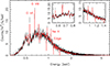 |
Fig. 11. Simulation with NewAthena/X-IFU (10 ks). Template model used (red line): best-fit continuum + wind model from ObsID 0655050101 (see Table 1 and Fig. A.5, top left panel). |
6. Conclusions
In this work we have described a deep observing campaign with XMM-Newton of a well-known ultra-luminous X-ray source, NGC 55 ULX-1, in order to corroborate the previous evidence of outflows in the high-resolution RGS spectra and to search for any trends between the accretion properties (e.g. luminosity, spectral hardness, and variability) and ejection properties (wind velocity, column density, and temperature). The combined time-average spectrum strengthened the previous detection confidence levels and provided more insight on the nature of the 1 keV feature usually seen in high-count CCD spectra of ULXs. The comparison between the results obtained at different epochs revealed that the wind responds to the variability of the underlying continuum, and these variations may be used to understand the actual accretion regime and the nature of the source. Future observations with high-throughput high spectral resolution facilities, such as NewAthena, will cement our understanding thanks to the possibility of tracing such trends on the short variability timescales of the accretion process.
Data availability
All data and software used in this work are publicly available from the XMM-Newton Science Archives (https://www.cosmos.esa.int/web/xmm-newton/xsa), (https://heasarc.gsfc.nasa.gov/). Our codes are also publicly available on GitHub (https://github.com/ciropinto1982).
Acknowledgments
We acknowledge funding from PRIN MUR 2022 SEAWIND 2022Y2T94C, supported by European Union – Next Generation EU, Mission 4 Component 1 CUP C53D23001330006, INAF Large Grant 2023 BLOSSOM F.O. 1.05.23.01.13 and the Italian Space Agency, contract ASI-INAF program I/004/11/4-6. The authors also thank Srimanta Banerjee for helpful discussions on accretion disc physics.
References
- Alston, W. N., Pinto, C., Barret, D., et al. 2021, MNRAS, 505, 3722 [NASA ADS] [CrossRef] [Google Scholar]
- Bachetti, M., Rana, V., Walton, D. J., et al. 2013, ApJ, 778, 163 [Google Scholar]
- Bachetti, M., Harrison, F. A., Walton, D. J., et al. 2014, Nature, 514, 202 [NASA ADS] [CrossRef] [Google Scholar]
- Barra, F., Pinto, C., Walton, D. J., et al. 2022, MNRAS, 516, 3972 [NASA ADS] [CrossRef] [Google Scholar]
- Barra, F., Pinto, C., Middleton, M., et al. 2024, A&A, 682, A94 [NASA ADS] [CrossRef] [EDP Sciences] [Google Scholar]
- Bianchi, S., Ponti, G., Muñoz-Darias, T., & Petrucci, P.-O. 2017, MNRAS, 472, 2454 [Google Scholar]
- Bowler, M. G. 2011, A&A, 534, A112 [NASA ADS] [CrossRef] [EDP Sciences] [Google Scholar]
- Cash, W. 1979, ApJ, 228, 939 [Google Scholar]
- D’Aì, A., Pinto, C., Del Santo, M., et al. 2021, MNRAS, 507, 5567 [CrossRef] [Google Scholar]
- Earnshaw, H. M., & Roberts, T. P. 2017, MNRAS, 467, 2690 [NASA ADS] [CrossRef] [Google Scholar]
- Evans, P. A., Beardmore, A. P., Page, K. L., et al. 2009, MNRAS, 397, 1177 [Google Scholar]
- Fiacconi, D., Pinto, C., Walton, D. J., & Fabian, A. C. 2017, MNRAS, 469, L99 [Google Scholar]
- Fürst, F., Walton, D. J., Harrison, F. A., et al. 2016, ApJ, 831, L14 [Google Scholar]
- Fürst, F., Walton, D. J., Heida, M., et al. 2018, A&A, 616, A186 [Google Scholar]
- Gehrels, N., Chincarini, G., Giommi, P., et al. 2004, ApJ, 611, 1005 [Google Scholar]
- Gladstone, J. C., Roberts, T. P., & Done, C. 2009, MNRAS, 397, 1836 [NASA ADS] [CrossRef] [Google Scholar]
- Gladstone, J. C., Copperwheat, C., Heinke, C. O., et al. 2013, ApJS, 206, 14 [NASA ADS] [CrossRef] [Google Scholar]
- Gu, L., Mao, J., Kaastra, J. S., et al. 2022, A&A, 665, A93 [NASA ADS] [CrossRef] [EDP Sciences] [Google Scholar]
- Gúrpide, A., Godet, O., Koliopanos, F., Webb, N., & Olive, J. F. 2021, A&A, 649, A104 [NASA ADS] [CrossRef] [EDP Sciences] [Google Scholar]
- Gúrpide, A., Parra, M., Godet, O., Contini, T., & Olive, J. F. 2022, A&A, 666, A100 [NASA ADS] [CrossRef] [EDP Sciences] [Google Scholar]
- Israel, G. L., Belfiore, A., Stella, L., et al. 2017, Science, 355, 817 [NASA ADS] [CrossRef] [Google Scholar]
- Kaastra, J. S. 2017, A&A, 605, A51 [NASA ADS] [CrossRef] [EDP Sciences] [Google Scholar]
- Kaastra, J. S., Mewe, R., & Nieuwenhuijzen, H. 1996, in UV and X-ray Spectroscopy of Astrophysical and Laboratory Plasmas, eds. K. Yamashita, & T. Watanabe, 411 [Google Scholar]
- King, A., Lasota, J.-P., & Middleton, M. 2023, New Astron. Rev., 96, 101672 [CrossRef] [Google Scholar]
- Kobayashi, H., Ohsuga, K., Takahashi, H. R., et al. 2018, PASJ, 70, 22 [NASA ADS] [Google Scholar]
- Kosec, P., Pinto, C., Walton, D. J., et al. 2018, MNRAS, 479, 3978 [NASA ADS] [Google Scholar]
- Kosec, P., Pinto, C., Reynolds, C. S., et al. 2021, MNRAS, 508, 3569 [NASA ADS] [CrossRef] [Google Scholar]
- Krolik, J. H., McKee, C. F., & Tarter, C. B. 1981, ApJ, 249, 422 [NASA ADS] [CrossRef] [Google Scholar]
- Lepore, M., Pinto, C., Tozzi, P., et al. 2025, A&A, 694, A115 [NASA ADS] [CrossRef] [EDP Sciences] [Google Scholar]
- Lodders, K., & Palme, H. 2009, Meteor. Planet. Sci. Suppl., 72, 5154 [Google Scholar]
- Marshall, H. L., Canizares, C. R., & Schulz, N. S. 2002, ApJ, 564, 941 [NASA ADS] [CrossRef] [Google Scholar]
- Middleton, M. J., Walton, D. J., Roberts, T. P., & Heil, L. 2014, MNRAS, 438, L51 [Google Scholar]
- Middleton, M. J., Walton, D. J., Fabian, A., et al. 2015a, MNRAS, 454, 3134 [Google Scholar]
- Middleton, M. J., Heil, L., Pintore, F., Walton, D. J., & Roberts, T. P. 2015b, MNRAS, 447, 3243 [Google Scholar]
- Middleton, M. J., Higginbottom, N., Knigge, C., Khan, N., & Wiktorowicz, G. 2022, MNRAS, 509, 1119 [Google Scholar]
- Miller, J. M., Mizumoto, M., Shidatsu, M., et al. 2025, ApJ, 988, L28 [Google Scholar]
- Neilsen, J., & Degenaar, N. 2023, arXiv e-prints [arXiv:2304.05412] [Google Scholar]
- Ohsuga, K., Mori, M., Nakamoto, T., & Mineshige, S. 2005, ApJ, 628, 368 [NASA ADS] [CrossRef] [Google Scholar]
- Pakull, M. W., Soria, R., & Motch, C. 2010, Nature, 466, 209 [Google Scholar]
- Peille, P., Barret, D., Cucchetti, E., et al. 2025, Exp. Astron., 59, 18 [Google Scholar]
- Petrucci, P. O., Bianchi, S., Ponti, G., et al. 2021, A&A, 649, A128 [NASA ADS] [CrossRef] [EDP Sciences] [Google Scholar]
- Pinto, C., & Walton, D. J. 2023, Ultra-Luminous X-Ray Sources: Extreme Accretion and Feedback (Singapore: Springer Nature), 345 [Google Scholar]
- Pinto, C., Middleton, M. J., & Fabian, A. C. 2016, Nature, 533, 64 [Google Scholar]
- Pinto, C., Alston, W., Soria, R., et al. 2017, MNRAS, 468, 2865 [Google Scholar]
- Pinto, C., Alston, W., Parker, M. L., et al. 2018, MNRAS, 476, 1021 [NASA ADS] [CrossRef] [Google Scholar]
- Pinto, C., Mehdipour, M., Walton, D. J., et al. 2020a, MNRAS, 491, 5702 [Google Scholar]
- Pinto, C., Walton, D. J., Kara, E., et al. 2020b, MNRAS, 492, 4646 [Google Scholar]
- Pinto, C., Soria, R., Walton, D. J., et al. 2021, MNRAS, 505, 5058 [NASA ADS] [CrossRef] [Google Scholar]
- Pintore, F., Esposito, P., Zampieri, L., Motta, S., & Wolter, A. 2015, MNRAS, 448, 1153 [Google Scholar]
- Pintore, F., Pinto, C., Rodriguez-Castillo, G., et al. 2025, A&A, 695, A238 [NASA ADS] [CrossRef] [EDP Sciences] [Google Scholar]
- Porquet, D., & Dubau, J. 2000, A&AS, 143, 495 [NASA ADS] [CrossRef] [EDP Sciences] [Google Scholar]
- Poutanen, J., Lipunova, G., Fabrika, S., Butkevich, A. G., & Abolmasov, P. 2007, MNRAS, 377, 1187 [NASA ADS] [CrossRef] [Google Scholar]
- Psaradaki, I., Costantini, E., Mehdipour, M., & Díaz Trigo, M. 2018, A&A, 620, A129 [NASA ADS] [CrossRef] [EDP Sciences] [Google Scholar]
- Robba, A., Pinto, C., Pintore, F., et al. 2022, MNRAS, 515, 4669 [Google Scholar]
- Soria, R., Motch, C., Read, A. M., & Stevens, I. R. 2004, A&A, 423, 955 [NASA ADS] [CrossRef] [EDP Sciences] [Google Scholar]
- Stobbart, A.-M., Roberts, T. P., & Wilms, J. 2006, MNRAS, 368, 397 [Google Scholar]
- Takeuchi, S., Ohsuga, K., & Mineshige, S. 2013, PASJ, 65, 88 [Google Scholar]
- Urquhart, R., & Soria, R. 2016, MNRAS, 456, 1859 [Google Scholar]
- van den Eijnden, J., Degenaar, N., Schulz, N. S., et al. 2019, MNRAS, 487, 4355 [Google Scholar]
- Waisberg, I., Dexter, J., Petrucci, P.-O., Dubus, G., & Perraut, K. 2019, A&A, 623, A47 [NASA ADS] [CrossRef] [EDP Sciences] [Google Scholar]
- Walton, D. J., Harrison, F. A., Grefenstette, B. W., et al. 2014, ApJ, 793, 21 [Google Scholar]
- Xrism Collaboration (Audard, M., et al.) 2025, Nature, 641, 1132 [Google Scholar]
- Xu, Y., Pinto, C., Rogantini, D., et al. 2023, MNRAS, 523, 2158 [NASA ADS] [CrossRef] [Google Scholar]
- Xu, Y., Gallo, L. C., Hagino, K., et al. 2025, PASJ, accepted [arXiv:2506.05273] [Google Scholar]
- Zhou, C., Feng, H., & Bian, F. 2023, ApJ, 955, 61 [Google Scholar]
Appendix A: Technical details
In this section, we include some technical details and plots that were excluded from the main body of the paper.
A.1. SED and plasma thermal stability
As mentioned in Sect. 3, no optical counterpart was detected in the XMM-Newton/OM data. However, we made sure that the exclusion of the optical/UV emission in our SED model has a negligible impact on the ionisation balance. As can be seen in Fig. A.1, the extrapolation of our best-fit model down to 0.002 keV results in a flux of 5 × 10⁻¹⁷ erg/s/cm2, which is a factor of 10 lower than that measured with MUSE (Zhou et al. 2023) and even lower than previous estimates with HST which showed a very faint optical counterpart beyond the reach of OM (HST magnitude ≳23, Gladstone et al. 2013).
For a comparison, we have also built a multi-wavelength SED (and computing the corresponding ionisation balance) by adding the HST optical data (see e.g. Gladstone et al. 2013; Zhou et al. 2023). For this task, we adopted a plasma density nH = 1010 cm−3 in coherence with the assumptions for photoiosation model scans which were suggested by the independent Gaussian modelling because the balance depends on the density (see e.g. Bianchi et al. 2017). There is no significant difference in the stability curves due to the weakness of the flux at optical-UV wavelengths (see Fig. A.1 dotted line) and the rather soft SED, which is a characteristic common to ultra-luminous X-ray sources (see Pinto & Walton 2023 and references therein).
In Fig. A.1, we also highlight, with thicker segments, the best fits of photoionised plasma models with emission lines (pion) and absorption lines (xabs) from Table 1 to check whether all solutions correspond to stable branches of the stability curves. This occurs for most components, with the exception of the slow/cool (vLOS = −0.05c and log ξ = 1.26) absorbing plasma that appears in the highest-flux ObsID (088396) and, at a lower significance, in the first observation. The solutions are labelled ‘warm’ and ‘cool’ to differentiate between the high and low ξ values in Table 1.
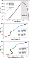 |
Fig. A.1. Spectral energy distribution (top panel), ionisation balance (middle panel), and stability curve (bottom panel). The band covered by XMM-Newton is shown in grey. Combined+V refers to the multi-wavelength SED built with XMM-Newton X-ray data and HST optical data. The ionisation balance and stability curves of the individual observations are not shown since they are almost superimposable. The best-fit ranges of the emission (pion) and absorption (xabs) line components obtained for the individual observations are shown as thicker segments (see Table 1). |
A.2. Spectra and fits of individual observations
In Fig. A.2, we show the spectra of each observation with the spectral continuum model overlaid. We adopted a double thermal model consisting of a cool (0.16–0.21 keV) blackbody and a warmer (0.7–0.9 keV) blackbody modified by coherent Compton scattering for the broader and harder component. These two components refer to the outer/cooler and inner/hotter super-Eddington inner disc, with the latter being slightly obscured due to the LOS inclination. More detail is provided in Sect. 4.1.1. In Fig. A.5, we show the best-fit continuum modelling of the individual observations with the addition of two photoionised plasma components to account for the emission (pion) and the absorption (xabs) lines. For more detail, see Sect. 4.2.
In Fig. A.3 we report the multi-dimensional grids of the spectra with different physical models (emission by collisional or photoionised plasmas and absorption by a photoionised plasma) with the same routine used in Sect. 4.1.3. The black contours refer to the confidence level estimated through MC simulations as described in Sect. 4.3.
In Fig. A.4, we show further increments when cie and xabs grids were run again for ObsID 0655050101 once the contribution of the primary solutions (i.e. those reported in Table 1 and Fig. 8-10) were included in the underlying baseline model. The very low ΔC show how the primary solution was able to describe most of the corresponding features found with the scans. Moreover, the presence of a low-velocity (−0.05c) absorption component although rather weak indicates presence of a multi-phase plasma as it was already discussed in P17 (see Fig. A.4, right panel).
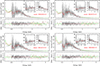 |
Fig. A.2. XMM-Newton spectra and continuum modelling of the individual observations. The labels are same as in Fig. 2. Only the first-order RGS spectrum is used due to the low statistics of the second-order individual spectra. |
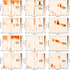 |
Fig. A.3. Physical model grids of the individual observations: CIE emission (left), PIE emission (middle), and PIE absorption (right). The black contours refer to significance levels from 3 to 5 σ with steps of 0.5 σ estimated with MC simulations (see Sect. 4.3). |
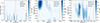 |
Fig. A.4. Physical model grids (zoom) of ObsID 0655050101 to the address the significance of secondary solutions (therefore the blue colour map): CIE emission (left), PIE absorption (part a, middle; part b, right). We note the much lower ΔC once each primary solution is taken into account. |
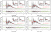 |
Fig. A.5. XMM-Newton spectra and best-fit photoionised emission–absorption model of the individual observations. The labels are same as in Fig. A.2. |
A.3. Monte Carlo simulations
In Fig. A.6, we reported with red bars the histogram of the ΔC-stat occurrences obtained from a deep grid of absorption models of photoionised plasma for 16,000 simulated spectra based on the continuum model of RGS+EPIC ObsID 0655050101. The stability of the histogram slope (−0.26) above about 5,000 simulated spectra enabled us to forecast the results for 1.5 × 10⁵ and 1.7 × 10⁶ simulations and probe the ΔC-stat corresponding to detections with confidence levels up to 4.5 and 5.0 σ (see vertical dotted lines). The confidence levels can also be found as black contours in Fig. A.3. The black and blue bars refer to the results obtained for grids of emission and absorption models applied on the real data for the same ObsID. For more detail, see Sect. 4.3.
A.4. Contribution of spectral components
In Fig. A.7, we show in detail the contribution of each spectral component in the best fit for each individual observation. To highlight the contribution of the xabs component we show the case where the simple continuum model was multiplied by the xabs (along with the ISM), i.e. the emission of the pion was removed.
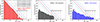 |
Fig. A.6. Monte Carlo simulations for significance estimates (left panel, red bars, template model: continuum model for ObsID 0655050101). Forecasts for more than 16,000 simulations are performed adopting a constant histogram slope. As a comparison the results for the xabs (middle panel, black bars) and the pion (right panel, blue bars) histograms for the real data are also shown. |
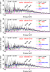 |
Fig. A.7. Detail of the main spectral components of the continuum (bb and mbb) and the plasma (xabs in absorption and pion in emission) zoomed in on the RGS spectra. The best-fit model of each spectrum is also shown in Table 1 and previously in Fig. A.5. The ISM contribution is present in each model. Labelled are the main ionic species for the soft X-ray emission in their rest frame (see also Fig. 2, 4 and 5). |
All Tables
All Figures
|
Fig. 1. Swift/XRT long-term light curve (top panel) and hardness ratio curve of NGC 55 ULX-1 (bottom panel). The hardness ratio is computed as the ratio of the counts in the 2−10 keV to 0.3−2 keV energy bands. The values for the four on-axis deep XMM-Newton observations are shown with horizontal lines and the times of the events with X markers followed by the corresponding ObsID. |
| In the text | |
|
Fig. 2. XMM-Newton combined spectra of ULX-1 obtained by stacking those from the four deep on-axis observations: RGS first-order (light blue) and second-order (black), EPIC-pn (grey), MOS 1 (red), and MOS 2 (green). |
| In the text | |
|
Fig. 3. XMM-Newton time-averaged (on-axis) spectra and continuum model. The labels are the same as in Fig. 2. The EPIC data were ignored in the range 0.5−1.8 keV in order to fully employ the high spectral resolution of RGS and decrease degeneracy between models of line emission and absorption. |
| In the text | |
|
Fig. 4. Gaussian line scan of the XMM-Newton time-averaged spectrum (top panel) and spectra of the individual observations. Labelled are the energy centroids of some of the most common X-ray spectral lines; Fe K refers to the Fe I fluorescence and the Fe XXV resonant lines. The grey vertical line indicates the separation between RGS and EPIC. The grey-shaded areas indicate the 3σ single-trial significance. |
| In the text | |
|
Fig. 5. XMM-Newton RGS time-averaged spectrum (order 1 in blue, order 2 in black) and Gaussian emission lines, zoomed in on the Mg-Ne K, Fe L, and O K edges. We note the weakness of the Fe lines, the stronger O VII forbidden line, and the tentative RRC profiles (with hints of photoionisation). |
| In the text | |
|
Fig. 6. XMM-Newton time-averaged grids of physical models. From top to bottom: CIE (cie model) emission, PIE (pion) emission, and (xabs) absorption. The black contours refer to significance levels from 3 to 5σ with steps of 0.5σ estimated with MC simulations (Sect. 4.3). |
| In the text | |
|
Fig. 7. O VII He-like triplet R (top) and G (bottom) ratio curves calculated from the time-averaged SED. The grey-shaded areas indicate the regions compatible with the results from the combined spectrum and the upper limits on the temperature and the density (see Sect. 5). |
| In the text | |
|
Fig. 8. Summary plot for the results relative to the xabs (photoionised absorber) model. The grey circles refer to the combined spectrum. |
| In the text | |
|
Fig. 9. Summary plot for the results relative to the pion (photoionised emitter) model. The grey circles refer to the combined spectrum. |
| In the text | |
|
Fig. 10. Summary plot for the results relative to the cie (collisionally ionised emitter) model. The grey circles refer to the combined spectrum. |
| In the text | |
|
Fig. 11. Simulation with NewAthena/X-IFU (10 ks). Template model used (red line): best-fit continuum + wind model from ObsID 0655050101 (see Table 1 and Fig. A.5, top left panel). |
| In the text | |
|
Fig. A.1. Spectral energy distribution (top panel), ionisation balance (middle panel), and stability curve (bottom panel). The band covered by XMM-Newton is shown in grey. Combined+V refers to the multi-wavelength SED built with XMM-Newton X-ray data and HST optical data. The ionisation balance and stability curves of the individual observations are not shown since they are almost superimposable. The best-fit ranges of the emission (pion) and absorption (xabs) line components obtained for the individual observations are shown as thicker segments (see Table 1). |
| In the text | |
|
Fig. A.2. XMM-Newton spectra and continuum modelling of the individual observations. The labels are same as in Fig. 2. Only the first-order RGS spectrum is used due to the low statistics of the second-order individual spectra. |
| In the text | |
|
Fig. A.3. Physical model grids of the individual observations: CIE emission (left), PIE emission (middle), and PIE absorption (right). The black contours refer to significance levels from 3 to 5 σ with steps of 0.5 σ estimated with MC simulations (see Sect. 4.3). |
| In the text | |
|
Fig. A.4. Physical model grids (zoom) of ObsID 0655050101 to the address the significance of secondary solutions (therefore the blue colour map): CIE emission (left), PIE absorption (part a, middle; part b, right). We note the much lower ΔC once each primary solution is taken into account. |
| In the text | |
|
Fig. A.5. XMM-Newton spectra and best-fit photoionised emission–absorption model of the individual observations. The labels are same as in Fig. A.2. |
| In the text | |
|
Fig. A.6. Monte Carlo simulations for significance estimates (left panel, red bars, template model: continuum model for ObsID 0655050101). Forecasts for more than 16,000 simulations are performed adopting a constant histogram slope. As a comparison the results for the xabs (middle panel, black bars) and the pion (right panel, blue bars) histograms for the real data are also shown. |
| In the text | |
|
Fig. A.7. Detail of the main spectral components of the continuum (bb and mbb) and the plasma (xabs in absorption and pion in emission) zoomed in on the RGS spectra. The best-fit model of each spectrum is also shown in Table 1 and previously in Fig. A.5. The ISM contribution is present in each model. Labelled are the main ionic species for the soft X-ray emission in their rest frame (see also Fig. 2, 4 and 5). |
| In the text | |
Current usage metrics show cumulative count of Article Views (full-text article views including HTML views, PDF and ePub downloads, according to the available data) and Abstracts Views on Vision4Press platform.
Data correspond to usage on the plateform after 2015. The current usage metrics is available 48-96 hours after online publication and is updated daily on week days.
Initial download of the metrics may take a while.