| Issue |
A&A
Volume 706, February 2026
|
|
|---|---|---|
| Article Number | A369 | |
| Number of page(s) | 9 | |
| Section | The Sun and the Heliosphere | |
| DOI | https://doi.org/10.1051/0004-6361/202556666 | |
| Published online | 20 February 2026 | |
Active chromospheric fibril singularity
Coordinated observations from Solar Orbiter, SST, and IRIS
1
Rosseland Centre for Solar Physics, University of Oslo P.O. Box 1029 Blindern N-0315 Oslo, Norway
2
Institute of Theoretical Astrophysics, University of Oslo P.O. Box 1029 Blindern N-0315 Oslo, Norway
3
NASA Goddard Space Flight Center, Heliophysics Science Division Greenbelt MD 20771, USA
4
Department of Physics and Astronomy, George Mason University Fairfax VA 22030, USA
5
Sorbonne Université, Observatoire de Paris – PSL, École Polytechnique, Institut Polytechnique de Paris, CNRS, Laboratoire de physique des plasmas (LPP) 4 Place Jussieu F-75005 Paris, France
6
Institute for Solar Physics, Dept. of Astronomy, Stockholm University, Albanova University Center 10691 Stockholm, Sweden
7
Statkraft AS Lysaker, Norway
8
Instituto de Astrofísica de Canarias E-38205 La Laguna Tenerife, Spain
9
Universidad de La Laguna, Dept. Astrofísica E-38206 La Laguna Tenerife, Spain
10
Max-Planck-Institut für Sonnensystemforschung Justus-von-Liebig-Weg 3 37077 Göttingen, Germany
★ Corresponding author: This email address is being protected from spambots. You need JavaScript enabled to view it.
Received:
30
July
2025
Accepted:
30
November
2025
Abstract
Context. The fine structures of the solar chromosphere, driven by photospheric motions, play a crucial role in the dynamics of solar magnetic fields. Many such structures have already been identified, such as fibrils, filament feet, and arch filament systems. Nevertheless, high-resolution observations show a wealth of structures whose nature remains elusive.
Aims. We observed a puzzling, unprecedented chromospheric fibril singularity in the close vicinity of a blow-out solar jet and a flaring loop. We aim to understand the magnetic nature of this singularity and the cause of its activity using coordinated high-resolution, multi-wavelength observations.
Methods. We aligned datasets from Solar Orbiter, SST, IRIS, and SDO. We re-projected the Solar Orbiter datasets to match the perspective of the Earth-based instruments and performed potential field extrapolations from Solar Orbiter/PHI data. We analysed the spatial and temporal evolution of the plasma structures and their link with the surface magnetic field. This led us to derive a model and scenario for the observed structures, which we explain in a general schematic representation.
Results. We have discovered a new feature: a singularity in the chromospheric fibril pattern. It forms in a weak magnetic-field corridor between two flux concentrations of equal sign, at the base of a vertically inverted-Y-shaped field-line pattern. In this specific case, some activity develops along the structure: first, a flaring loop at one end, and second, a blow-out jet at the other end, where a coronal null point was present and associated with a chromospheric saddle point located on the fibril singularity. The observations suggest that both active phenomena are initiated by converging photospheric moat flows that exert pressure on this fibril singularity.
Key words: Sun: activity / Sun: chromosphere / Sun: corona / Sun: photosphere
© The Authors 2026
 Open Access article, published by EDP Sciences, under the terms of the Creative Commons Attribution License (https://creativecommons.org/licenses/by/4.0), which permits unrestricted use, distribution, and reproduction in any medium, provided the original work is properly cited.
This article is published in open access under the Subscribe to Open model. This email address is being protected from spambots. You need JavaScript enabled to view it. to support open access publication.
1. Introduction
Fine structures in the solar chromosphere are believed to be aligned with the magnetic field. Consequently, high-resolution chromospheric observations provide a powerful indirect diagnostic for exploring the geometry and topology of magnetic fields; in particular, Hα observations serve as an effective proxy for chromospheric magnetograms (Filippov 1995). Recent advances in ground- and space-based observational capabilities have markedly improved spatial, temporal, and spectral resolution, offering unprecedented insights into the dynamic fine-scale structure of the solar chromosphere and its coupling to the higher layers of the solar atmosphere.
Chromospheric fibrils, prominently observed in Hα, form a dense canopy at chromospheric heights. Along these fibrils solar jets are often observed. These jets are impulsive, collimated plasma ejections (Shibata et al. 1992; Nisticò et al. 2009; Sterling et al. 2015; Joshi et al. 2024a), and often involve plasma at cool chromospheric temperatures, commonly referred to as surges (Schmieder et al. 1995; Shen et al. 2012; Uddin et al. 2012; Nóbrega-Siverio et al. 2016, 2017; Shen et al. 2017; Joshi et al. 2020a, 2024b). Magnetic reconnection in the solar corona generates high-velocity, hot jets visible in X-ray or extreme-ultraviolet (EUV) wavelengths, while reconnection occurring lower in the chromosphere results in cooler Hα surges. These processes and the different types of jets are described in detail in the reviews of, for example, Raouafi et al. (2016), Shen (2021), and Schmieder et al. (2022). These jets are broadly classified as standard and blow-out jets (Moore et al. 2010; Shen et al. 2012; Sterling et al. 2015; Chandra et al. 2017; Kumar et al. 2019; Schmieder 2022). Blow-out jets form a more dynamic subclass of solar jets, arising from the eruption of small filaments, with some events showing associations with coronal mass ejections (Shen et al. 2012; Duan et al. 2019; Shen et al. 2019; Joshi et al. 2020b; Duan et al. 2024). These jets typically originate from a distinct magnetic topology known as an ‘X-point’ or ‘null point’, where magnetic field lines converge or diverge (Pariat et al. 2009). This configuration facilitates the rapid release of magnetic energy, driving the formation of a jet. In an insightful study, Titov et al. (2011) explored reconnection along a null line. In this scenario, instead of an open-field corridor, different reconnection regions can be connected by a singular line corresponding to the separatrix footprint. In the presence of magnetic null points, the connectivity of the magnetic field is determined by the skeleton of the field configuration. When nulls vanish below the photosphere, these skeletons transform into quasi-separatrix layers (Restante et al. 2009), where current sheets can naturally form (Aulanier et al. 2005).
Recently, fine structures related to jets have been observed using the advanced instrumentation of Solar Orbiter (Müller et al. 2020). High-resolution observations from the Extreme Ultraviolet Imager (EUI; Rochus et al. 2020) have enabled the study of these phenomena on much smaller scales (Mandal et al. 2022; Panesar et al. 2023; Nóbrega-Siverio et al. 2025), resolving features down to spatial scales of a few hundred kilometres (Chitta et al. 2023; Poirier et al. 2025). Solar Orbiter observations, together with chromospheric data from ground-based instruments, are crucial for examining whether solar jets always conform to conventional reconnection scenarios. This motivated us to conduct a coordinated observational campaign using multiple instruments, during which we detected repeated solar jets. The chromospheric environment is particularly striking, as fine-scale fibrils emerge and play a crucial role in the propagation of brightenings near the base of a blow-out jet. We present observations in which the fibril pattern shows an unusual ‘parting hairstyle’ appearance, giving it a distinctive and singular character. The morphology and orientation of chromospheric fibrils allow us to infer the magnetic field geometry in a region where direct, high-resolution magnetic field measurements are notoriously difficult to obtain.
2. Observations and methods
On 20 October 2023, active region (AR) 13468 was observed by a unique combination of observatories: Solar Orbiter at a heliocentric distance of 0.41 AU, the Interface Region Imaging Spectrograph (IRIS; De Pontieu et al. 2014), the Swedish 1-m Solar Telescope (SST; Scharmer et al. 2003) on La Palma, and the Solar Dynamics Observatory (SDO; Pesnell et al. 2012). An extensive range of the active region atmosphere was covered with high-resolution coronal imaging by the EUI/High Resolution Imager (HRI) 174 Å, transition region imaging by the IRIS slit-jaw channel SJI 1400 Å, and chromospheric Hα and photospheric wide-band imaging by the SST. Solar Orbiter’s Polarimetric and Helioseismic Imager (PHI; Solanki et al. 2020) provided photospheric magnetic field maps (see Fig. 1 for wider context, and Fig. 2). Details on the observations and instruments are provided in Appendix A. To investigate the magnetic field topology we performed a potential field extrapolation on the photospheric magnetic field data from PHI.
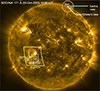 |
Fig. 1. Outline of the areas covered by different instruments, drawn on a full-disc AIA 171 Å image. The diagram in the top right indicates the viewing angle (44°) and heliocentric distance (0.41 AU) of Solar Orbiter compared with SST, IRIS, and SDO, which all observe along the Earth-Sun viewing line. |
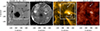 |
Fig. 2. Observations from Solar Orbiter (reprojected to Earth’s view), SST, and IRIS showing a fibril singularity and a blow-out jet around 09:40 UT. The Solar Orbiter/PHI magnetogram (left panel) shows the sunspot’s moat flow, containing small-scale magnetic patches (see the attached animation). The black arrow in the SST panel indicates the chromospheric material ejected from the peeling of the arch filament system. The white box shows the field of view of Fig. 3. This figure is associated with an online animation (PHI+SST+EUI+IRIS_2023-10-20_fullfov.mp4). |
We performed a fast Fourier transformation-based potential field extrapolation (Nakagawa & Raadu 1972; Alissandrakis 1981) on the photospheric BLOS data from PHI. This choice was made to circumvent challenges and inaccuracies arising from the ambiguity resolution of the full vector magnetic field, allowing us to work with a straightforward and well-established potential field model. The extrapolation was performed over the full PHI field of view (FOV), resulting in a box size of 1536 × 1536 × 384 grid points, which approximately corresponds to a domain size of 228 Mm × 228 Mm × 57 Mm. The bottom boundary used for extrapolation was also checked to ensure flux balance, allowing the resultant extrapolated magnetic field to closely satisfy the divergence-free condition. The mean value of BLOS for this region is −2.3 G, which is well below the noise level of about 10 G. To visualise the extrapolated magnetic field lines in 3D, we used the VAPOR software (Li et al. 2019). In Fig. 3, we trace the magnetic field lines near the base of the jet through bidirectional field-line integration by randomly placing the seed points within a small volume biased towards smaller values of |B|. This approach allowed us to trace the field lines closely following the separator connecting the null points.
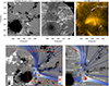 |
Fig. 3. Zoomed-in view of the area outlined by the white box in Fig. 2. A strong moat flow is observed near the jet base and is marked with a black arrow in panel a. Four main positive- and negative-polarity patches are labelled as P1, P2, N1, and N2 respectively. The blow-out jet in the coronal EUV 174 Å image, associated with a chromospheric surge in Hα, is indicated with grey arrow in panels b and c. Fibrils and the ‘X’-shaped saddle-point structure are marked in the Hα image. A flaring loop associated with the chromospheric fibril singularity is shown in EUI and Hα. Potential-field extrapolations on the PHI magnetogram are shown in panels d–e. In panel d, the yellow arrow indicates the jet base, which consists of a fan-spine configuration with a null point and associated outer spine towards the west (black arrow). A zoomed-in version is shown in panel e, where several inverted ‘Y’ structures are shown from the weak magnetic corridor between N1 and N2. |
3. Chromospheric singularity, flaring loop, and blow-out jet
Two distinct events occurred in AR 13468: a blow-out coronal jet and a flaring loop along a long filamentary structure, which we refer to as an active fibril singularity. Its characteristics and origin are explored in detail below.
The blow-out jet lies in close proximity to the negative polarity sunspot, a region that produced multiple jets over time. In particular, we focus on the blow-out coronal jet launched around 09:37 UT, which was simultaneously observed by the SST. The PHI magnetograms clearly show the moat flow surrounding the sunspot, that is, the persistent outflow of magnetic patches away from the sunspot (see Fig. 2 and associated animation). The moat flow transported magnetic flux towards a strong positive polarity patch near (x, y) = (−370″, −250″). Figure A.2 illustrates how a negative polarity patch collides with this positive patch prior to the start of a blow-out jet. The base of the jet consists of arch filament systems (AFSs) that were oriented perpendicular to the small negative polarities of the moat flow and the positive boundary. This AFS is clearly visible in the Hα observations (marked with the black arrow in Fig. 2). After the AFS became visible in Hα, the jet base became bright in EUI 174 Å and in IRIS SJI 1400 Å Si IV. The blow-out jet became very prominent in EUI 174 Å and was also visible across all other temperature diagnostics. The EUI images show narrow threads and fine structures in the jet. There are also distinct, high-contrast dark structures inside the blow-out jet that may be associated with the surge that is prominently visible in the Hα image (grey arrow in Fig. 3). This surge results from the peeling of the AFS (Joshi et al. 2024b), or from a mini-filament eruption process (Sterling et al. 2015; Shen 2021).
Interestingly, we observe the appearance of a very thin structure that extends northwards, orthogonal to the jet’s direction of propagation. We refer to this structure as a flaring loop in the EUI 174 Å panel in Fig. 3, where it is particularly bright. To investigate the nature of the flaring loop, we analysed multi-wavelength observations from SDO/AIA in the 171, 193, 131, and 94 Å channels, focusing on the temporal evolution of the intensity at a selected location within the loop. The normalised intensity light curves exhibit an asymmetric flare-like profile, characterised by a distinct heating phase followed by a gradual cooling phase (see Fig. 4). The intensity was measured within the box indicated in Fig. A.1, over the period from 09:35 to 10:00 UT. All AIA channels show an intensity peak around 09:46 UT, followed by a rapid decline in intensity after 09:48 UT, consistent with post-flare cooling. The emission in the hotter AIA channels (94 Å and 131 Å) rises earlier and decays more rapidly than in the cooler channels, consistent with earlier findings on flare plasma (Sun et al. 2013; Dai et al. 2013). This flaring loop structure is also present in other diagnostics: fainter in the transition region SJI 1400 Å Si IV (see Fig. 2) and as a long and narrow dark fibril in chromospheric Hα observations. Over the 100-minute sequence of the observation (see animation associated with Fig. 2), three flaring loops and three jets are observed along the singularity, showing their recurrent behaviour (see Fig. A.3). We focus on the first flaring loop that occurs around the same time as the blow-out jet (09:40 UT). This flaring loop appears to originate from the main jet base, which is the region where the moat flow collides with the large positive polarity patch in the PHI magnetograms. It appears along a weak magnetic corridor between two large negative polarity patches that are labelled N1 and N2 in Fig. 3. Just below the flaring loop and above the jet base, an X-like structure or ‘saddle point’ is visible in chromospheric observations (indicated by a white arrow in Fig. 3b). The term saddle point is adopted from Filippov (1995).
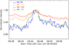 |
Fig. 4. Intensity light curves at the flaring loop location in different AIA channels. The curves display a flare-like evolution, with a rapid heating phase that is most pronounced in the hotter channels, and a cooling phase after the peak around 09:46 UT that is slower in the cooler channels. The position of the box used to compute the intensity is indicated in Fig. A.1. |
Examining the evolution of the magnetic field in the PHI magnetograms, we observe several magnetic polarities moving from the large sunspot towards the prominent negative polarity patch N1. These magnetic polarities, labelled C1, C2, C3, and C4 in Fig. A.4, illustrate the dynamic evolution of small-scale polarities near the main sunspot. The small polarities appear to emerge and propagate through a weak magnetic corridor (extending between N1 and N2), leading to enhanced flux convergence. For instance, the displacement of polarity C1 between 09:05 UT (Fig. A.4a) and 09:55 UT (Fig. A.4f) shows a clear northwards motion, as the arrow tip approaches the negative patch at the later time. Similarly, the motion of C4 is evident between panels e and f, while C2 shows the fading of a small positive patch at 09:15 UT, which reappears about 40 minutes later as a more circular feature that has migrated towards the weak magnetic corridor. Consequently, magnetic flux converges more intensely in the vicinity of the singularity.
4. Key findings from observations and magnetic modelling
A key finding of this study is the identification of an active chromospheric singularity along which a thin flaring loop oriented perpendicular to the blow-out jet (see the animation at 09:36:02). The flaring loop observed around 09:40:01 is both spatially and temporally aligned with the fibril singularity detected in Hα observations. A similar alignment is again evident later, at 09:53:41 and 10:45:33, with no other activity detected in the surrounding region. Therefore, we infer that this phenomenon is closely linked to the fibril singularity, which lies within the weak magnetic field corridor between N1 and N2. Morphologically, the fibrils appear to converge almost horizontally on both sides of this singularity, whereas along the line itself no fibrils are visible, at least not from above. This makes the line stand out as a unique feature, seemingly devoid of fibrils.
Potential field extrapolation confirms that the blow-out jet originates from a configuration with a characteristic fan-spine topology (with a null-point location), with open field lines extending westwards. The magnetic field rooted in the main polarities N1 and N2 is vertical, with a weak magnetic field corridor between them. These small positive patches are observed in the PHI magnetograms; however, they are too weak to result in extrapolations that provide unambiguous evidence of a null-like location. Notably, multiple inverted ‘Y’-shaped structures appear within this weak magnetic corridor (see Figs. 3d, e) through the long open field lines closing at the positive polarity. The long, dark filamentary structure in the SST observations represents a chromospheric fibril singularity. A chromospheric saddle point at one end of the fibril singularity is visible in the SST Hα images in Fig. 3b. Given the confirmation from observations and extrapolation, we suggest that the propagation of brightening northwards along the flaring loop follows this path, driven by converging motions that exert pressure on this region.
Figure 5 presents a schematic illustration of the magnetic environment of this case. However, this sketch is not intended to explain this specific observation only. The moat flow from the sunspot towards the surrounding negative polarity regions is indicated by black arrows. Two dominant magnetic polarities (grey ellipses) are connected via chromospheric fibrils. Some of these horizontal magnetic fields correspond to fibrils observed in Hα observations along the weak-field corridor. However, no such fibrils are seen between the two-flux concentrations N1 and N2 in the north. It is arguable that, given the geometry of the photospheric Bz, this horizontal field distribution should be present throughout the magnetic corridor, which we simplified in the sketch in Fig. 5. Dashed orange lines depict the fan surface of the null point associated with the blow-out jet. Consistent with the magnetic extrapolation, this surface is anchored at the jet base over the positive polarity P1. A series of parallel inverted ‘Y’-shaped structures appear rooted in a configuration similar to the main null, forming a complex magnetic topology. The fibril singularity, indicated by the magenta line, runs through this weak magnetic corridor between N1 and N2, intersecting the chain of inverted ‘Y’-shaped structures. This fibril singularity is a path along which the horizontal magnetic field emanating from N1 and N2 converges and meets. Hence, it is a unique and discontinuous linear structure in chromospheric fibrils. The brightening propagates along the flaring loop and appears to be connected to a small positive polarity at the top, as identified in the PHI magnetogram (Figs. 3a, d, and e). This connection is also supported by the extrapolated long, closed loops.
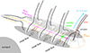 |
Fig. 5. Schematic representation of the observations. The two colliding regions of negative polarity are overlaid with chromospheric fibrils, shown in brown. The flaring loop along the fibril singularity is indicated by a curved orange arrow pointing left. The fibril singularity line is shown in magenta, with a saddle point at one end indicated in green. A saddle point is shown at the boundary between fan surfaces and the fibril singularity. Multiple inverted ‘Y’ structures along the fibril singularity are illustrated with parallel black colour behind the main null-point structure at the jet base. |
In summary, we propose the following scenario: continuous moat flows from the large negative sunspot result in converging magnetic flows between polarities of equal sign, N1 and N2. This leads to compression of the weak magnetic field between N1 and N2. It is plausible that this flow compressed the chromospheric fibril singularity, resulting in the formation of a current layer along the inverted ‘Y’-shaped structures. The continuous moat flow also forms a null-point structure with a blow-out jet ejection. The null point and the active fibril singularity are magnetically separated from the saddle point observed in the chromosphere.
5. Conclusions
We have discovered a new feature: an active singularity in the chromospheric fibril pattern, formed in a weak magnetic corridor. An observed saddle point at chromospheric heights forms at one end of this singularity and separates the field lines that converge towards the null point at the base of a blow-out jet from those directed towards the fibril singularity. Magnetic reconnection is triggered at the interface between the fan separatrix and this saddle point. This reconnection produces the separator field line, which is observed as the fibril singularity. Our observations support the idea proposed by Filippov (1995) that topological singularities in chromospheric structures are closely associated with solar activity. The ‘X’-type structure (saddle point) observed at the chromospheric level has been reported in several ground-based observations and interpreted as the projection of a coronal null point (Shen et al. 2019). Indeed, magnetic field lines on the edge of the fan footpoint can display a saddle-point structure, especially when the field lines outside the fan have inverted ‘Y’-shaped structures. In this configuration, where minimal magnetic flux is present between the two concentrations, the configuration corresponds to a true separatrix or a quasi-separatrix layer.
In our case, the weak vertical magnetic field between the main negative polarities is filled with horizontal fields that converge towards each other at the centre of the weak magnetic corridor. The field lines from the equal-sign magnetic polarities diverge locally from their centres, producing horizontal fields along their flanks and forming vertically inverted ‘Y’-shaped configurations. Although this is not a true topological structure, it nevertheless represents a distinct geometrical configuration. Such configurations naturally give rise to quasi-separatrix layer footpoints (see, e.g. Fig. 5 of Restante et al. 2009).
Our findings highlight the important role of chromospheric fine structures and offer new insights into the coupling between photospheric motions and coronal activity. In the future, coordinated multi-instrument campaigns will be essential to further investigate the concept of the fibril singularity and its role in solar jet dynamics.
Data availability
Movies associated with Figs. 2 and A.1 are available at https://www.aanda.org
Acknowledgments
The Swedish 1-m Solar Telescope (SST) is operated on the island of La Palma by the Institute for Solar Physics of Stockholm University in the Spanish Observatorio del Roque de los Muchachos of the Instituto de Astrofísica de Canarias. The SST is co-funded by the Swedish Research Council as a national research infrastructure (registration number 4.3-2021-00169). IRIS is a NASA small explorer mission developed and operated by LMSAL, with mission operations executed at NASA Ames Research Center and major contributions to downlink communications funded by ESA and the Norwegian Space Agency. SDO observations are courtesy of NASA/SDO and the AIA science teams. Solar Orbiter (SolO) is a space mission of international collaboration between ESA and NASA, operated by ESA. The EUI instrument was built by CSL, IAS, MPS, MSSL/UCL, PMOD/WRC, ROB, LCF/IO with funding from the Belgian Federal Science Policy Office (BELSPO/PRODEX PEA 4000134088); the Centre National d’Etudes Spatiales (CNES); the UK Space Agency (UKSA); the Bundesministerium für Wirtschaft und Energie (BMWi) through the Deutsches Zentrum für Luft- und Raumfahrt (DLR); and the Swiss Space Office (SSO). The German contribution to SO/PHI is funded by the BMWi through DLR and by MPG central funds. The Spanish contribution is funded by AEI/MCIN/10.13039/501100011033/ and European Union “NextGenerationEU/PRTR” (RTI2018-096886-C5, PID2021-125325OB-C5, PCI2022-135009-2, PCI2022-135029-2) and ERDF “A way of making Europe”; “Center of Excellence Severo Ochoa” awards to IAA-CSIC (SEV-2017-0709, CEX2021-001131-S); and a Ramón y Cajal fellowship awarded to DOS. The French contribution is funded by CNES. This research is supported by the Research Council of Norway, project number 325491, and through its Centres of Excellence scheme, project number 262622. The work of GA was funded by the Appel à Proposition de Recherche of CNES/SHM and by the Action Thématique Soleil-Terre (ATST) of CNRS/INSU PN Astro, also funded by CNES, CEA, and ONERA. R.J. and D.N.S. gratefully acknowledge the Solar Orbiter/EUI Guest Investigator program, where discussions related to this work took place during their two research stays at the Royal Observatory of Belgium. This project has received funding from Swedish Research Council (2021-05613), Swedish National Space Agency (2021-00116). A.P. and D.N.S. acknowledge support from the European Research Council through the Synergy Grant number 810218 (“The Whole Sun”, ERC-2018-SyG). N.P. acknowledges funding from the Research Council of Norway, project no. 324523. The use of UCAR’s VAPOR software (www.vapor.ucar.edu) is gratefully acknowledged. We made much use of NASA’s Astrophysics Data System Bibliographic Services.
References
- Alissandrakis, C. E. 1981, A&A, 100, 197 [NASA ADS] [Google Scholar]
- Auchère, F., Soubrié, E., Pelouze, G., & Buchlin, É. 2023, A&A, 670, A66 [NASA ADS] [CrossRef] [EDP Sciences] [Google Scholar]
- Aulanier, G., Pariat, E., & Démoulin, P. 2005, A&A, 444, 961 [NASA ADS] [CrossRef] [EDP Sciences] [Google Scholar]
- Chandra, R., Mandrini, C. H., Schmieder, B., et al. 2017, A&A, 598, A41 [NASA ADS] [CrossRef] [EDP Sciences] [Google Scholar]
- Chitta, L. P., Zhukov, A. N., Berghmans, D., et al. 2023, Science, 381, 867 [NASA ADS] [CrossRef] [Google Scholar]
- Dai, Y., Ding, M. D., & Guo, Y. 2013, ApJ, 773, L21 [Google Scholar]
- de la Cruz Rodríguez, J., Löfdahl, M. G., Sütterlin, P., Hillberg, T., & Rouppe van der Voort, L. 2015, A&A, 573, A40 [NASA ADS] [CrossRef] [EDP Sciences] [Google Scholar]
- De Pontieu, B., Title, A. M., Lemen, J. R., et al. 2014, Sol. Phys., 289, 2733 [Google Scholar]
- Duan, Y., Shen, Y., Chen, H., & Liang, H. 2019, ApJ, 881, 132 [Google Scholar]
- Duan, Y., Shen, Y., Tang, Z., Zhou, C., & Tan, S. 2024, ApJ, 968, 110 [Google Scholar]
- Filippov, B. P. 1995, A&A, 303, 242 [Google Scholar]
- Gandorfer, A., Grauf, B., Staub, J., et al. 2018, SPIE Conf. Ser., 10698, 1403 [Google Scholar]
- Joshi, R., Chandra, R., Schmieder, B., et al. 2020a, A&A, 639, A22 [NASA ADS] [CrossRef] [EDP Sciences] [Google Scholar]
- Joshi, R., Wang, Y., Chandra, R., et al. 2020b, ApJ, 901, 94 [NASA ADS] [CrossRef] [Google Scholar]
- Joshi, R., Aulanier, G., Radcliffe, A., et al. 2024a, A&A, 687, A172 [NASA ADS] [CrossRef] [EDP Sciences] [Google Scholar]
- Joshi, R., Rouppe van der Voort, L., Schmieder, B., et al. 2024b, A&A, 691, A198 [NASA ADS] [CrossRef] [EDP Sciences] [Google Scholar]
- Kumar, P., Karpen, J. T., Antiochos, S. K., Wyper, P. F., & DeVore, C. R. 2019, ApJ, 885, L15 [Google Scholar]
- Lemen, J. R., Title, A. M., Akin, D. J., et al. 2012, Sol. Phys., 275, 17 [Google Scholar]
- Li, S., Jaroszynski, S., Pearse, S., Orf, L., & Clyne, J. 2019, Atmosphere, 10, 488 [NASA ADS] [CrossRef] [Google Scholar]
- Löfdahl, M., Hillberg, T., de la Cruz Rodríguez, J., et al. 2021, A&A, 653, A68 [NASA ADS] [CrossRef] [EDP Sciences] [Google Scholar]
- Mandal, S., Chitta, L. P., Peter, H., et al. 2022, A&A, 664, A28 [NASA ADS] [CrossRef] [EDP Sciences] [Google Scholar]
- Moore, R. L., Cirtain, J. W., Sterling, A. C., & Falconer, D. A. 2010, ApJ, 720, 757 [Google Scholar]
- Müller, D., St. Cyr, O. C., Zouganelis, I., et al. 2020, A&A, 642, A1 [Google Scholar]
- Nakagawa, Y., & Raadu, M. A. 1972, Sol. Phys., 25, 127 [NASA ADS] [CrossRef] [Google Scholar]
- Nisticò, G., Bothmer, V., Patsourakos, S., & Zimbardo, G. 2009, Sol. Phys., 259, 87 [CrossRef] [Google Scholar]
- Nóbrega-Siverio, D., Moreno-Insertis, F., & Martínez-Sykora, J. 2016, ApJ, 822, 18 [Google Scholar]
- Nóbrega-Siverio, D., Martínez-Sykora, J., Moreno-Insertis, F., & Rouppe van der Voort, L. 2017, ApJ, 850, 153 [CrossRef] [Google Scholar]
- Nóbrega-Siverio, D., Joshi, R., Sola-Viladesau, E., Berghmans, D., & Lim, D. 2025, A&A, 702, A188 [NASA ADS] [CrossRef] [EDP Sciences] [Google Scholar]
- Panesar, N. K., Hansteen, V. H., Tiwari, S. K., et al. 2023, ApJ, 943, 24 [NASA ADS] [CrossRef] [Google Scholar]
- Pariat, E., Antiochos, S. K., & DeVore, C. R. 2009, ApJ, 691, 61 [Google Scholar]
- Pesnell, W. D., Thompson, B. J., & Chamberlin, P. C. 2012, Sol. Phys., 275, 3 [Google Scholar]
- Poirier, N., Danilovic, S., Kohutova, P., et al. 2025, A&A, 696, A125 [NASA ADS] [CrossRef] [EDP Sciences] [Google Scholar]
- Raouafi, N. E., Patsourakos, S., Pariat, E., et al. 2016, Space Sci. Rev., 201, 1 [Google Scholar]
- Restante, A. L., Aulanier, G., & Parnell, C. E. 2009, A&A, 508, 433 [NASA ADS] [CrossRef] [EDP Sciences] [Google Scholar]
- Rochus, P., Auchère, F., Berghmans, D., et al. 2020, A&A, 642, A8 [NASA ADS] [CrossRef] [EDP Sciences] [Google Scholar]
- Scharmer, G., Bjelksjö, K., Korhonen, T., Lindberg, B., & Petterson, B. 2003, SPIE Conf. Ser., 4853, 341 [NASA ADS] [Google Scholar]
- Scharmer, G. B., Narayan, G., Hillberg, T., et al. 2008, ApJ, 689, L69 [Google Scholar]
- Scharmer, G. B., Löfdahl, M. G., Sliepen, G., & de la Cruz Rodríguez, J. 2019, A&A, 626, A55 [NASA ADS] [CrossRef] [EDP Sciences] [Google Scholar]
- Scharmer, G. B., Sliepen, G., Sinquin, J. C., et al. 2024, A&A, 685, A32 [NASA ADS] [CrossRef] [EDP Sciences] [Google Scholar]
- Scherrer, P. H., Schou, J., Bush, R. I., et al. 2012, Sol. Phys., 275, 207 [Google Scholar]
- Schmieder, B. 2022, Front. Astron. Space Sci., 9, 820183 [NASA ADS] [CrossRef] [Google Scholar]
- Schmieder, B., Shibata, K., van Driel-Gesztelyi, L., & Freeland, S. 1995, Sol. Phys., 156, 245 [NASA ADS] [CrossRef] [Google Scholar]
- Schmieder, B., Joshi, R., & Chandra, R. 2022, Adv. Space Res., 70, 1580 [NASA ADS] [CrossRef] [Google Scholar]
- Shen, Y. 2021, Proc. Roy. Soc. London Ser. A, 477, 217 [NASA ADS] [Google Scholar]
- Shen, Y., Liu, Y., Su, J., & Deng, Y. 2012, ApJ, 745, 164 [NASA ADS] [CrossRef] [Google Scholar]
- Shen, Y., Liu, Y. D., Su, J., Qu, Z., & Tian, Z. 2017, ApJ, 851, 67 [NASA ADS] [CrossRef] [Google Scholar]
- Shen, Y., Qu, Z., Zhou, C., et al. 2019, ApJ, 885, L11 [NASA ADS] [CrossRef] [Google Scholar]
- Shibata, K., Nozawa, S., & Matsumoto, R. 1992, PASJ, 44, 265 [NASA ADS] [Google Scholar]
- Solanki, S. K., del Toro Iniesta, J. C., Woch, J., et al. 2020, A&A, 642, A11 [NASA ADS] [CrossRef] [EDP Sciences] [Google Scholar]
- Sterling, A., Moore, R., Falconer, D., & Adams, M. 2015, Nature, 523, 437 [NASA ADS] [CrossRef] [Google Scholar]
- Sun, X., Hoeksema, J. T., Liu, Y., et al. 2013, ApJ, 778, 139 [Google Scholar]
- The SunPy Community (Barnes, W., et al.) 2020, ApJ, 890, 68 [NASA ADS] [CrossRef] [Google Scholar]
- Titov, V., Mikić, Z., Linker, J., Lionello, R., & Antiochos, S. 2011, ApJ, 731, 111 [NASA ADS] [CrossRef] [Google Scholar]
- Uddin, W., Schmieder, B., Chandra, R., et al. 2012, ApJ, 752, 70 [NASA ADS] [CrossRef] [Google Scholar]
- Van Noort, M., Rouppe van der Voort, L., & Löfdahl, M. 2005, Sol. Phys., 228, 191 [NASA ADS] [CrossRef] [Google Scholar]
Appendix A: Observations
The observations were acquired as part of Solar Orbiter remote sensing window 11 (RSW11) in the period 11 to 22 October 2023. On 20 October 2023, Solar Orbiter was running an observing program (SOOP) that had as its main science objective to study flows and waves inside sunspots. The target was active region NOAA 13468. Solar Orbiter was at a heliocentric distance of 0.41 au which means that its solar observations have a light travel time difference of about 294 s as compared to Earth. As seen from Solar Orbiter, 1″ on the Sun corresponded to 296 km (as compared to 723 km as seen from Earth). Solar Orbiter was positioned at Stonyhurst longitude −42.2° and latitude +6.7°. The angle between the Earth-Sun and Solar Orbiter-Sun viewing lines was 44°. Due to this difference in viewing, the apparent size of the classical jet is quite different in the AIA 171 Å and EUI 174 Å images. As seen from Solar Orbiter, this jet reaches a maximum extent of about 50 Mm. In the AIA 171 Å images, the jet is shorter than 18 Mm (see Fig. A.1). The long axis of the jet has only a small angle with the line-of-sight from Earth and SDO, while from Solar Orbiter, the jet is viewed much more from the side. For a better comparison, the Solar Orbiter’s dataset has been reprojected to the Earth view direction using the reprojection routines of Sunpy (The SunPy Community 2020).
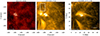 |
Fig. A.1. Blow-out jet at the time around maximum extent in IRIS SJI 1400 Å, AIA 171 Å, and EUI/HRIEUV 174 Å. The rectangular white box highlighted in the middle panel was used to compute the intensity variation presented in Fig. 4. The EUI image is shown without reprojection to the Earth viewing direction. An animation of this figure is available in the online material (AIA171+EUI+IRIS_2023-10-20_jet.mp4). |
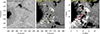 |
Fig. A.2. Reconnection regions and rapid motion of photospheric magnetic fields close to the sunspot. In Hα blue wing (left panel) the reconnection sites are outlined with blue contours, where enhanced Hα wing emission mark the location of Ellerman Bombs. The intensity at these locations is 1.45 times the intensity of the reference quiet Sun spectrum. The middle panel shows the cotemporal and aligned PHI BLOS map. Yellow circles mark the locations of these reconnection points. The right panel shows, at each pixel, the extremum of BLOS over 1 h before the onset of the jet generated from the original PHI data. Red contours mark pixels that have |BLOS|> 100 G for both polarities during the 1 h sequence. |
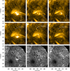 |
Fig. A.3. Recurrent blow-out jets and flaring loop along the fibril singularity in EUI/HRIEUV 174 Å (top and middle row) and SST/Hα (bottom row) observations. These activities along the fibril singularity occur at three different times along the whole duration of the coordinated observations (see the animation associated with Fig. 2) as shown in the middle row. Sometimes these are closely associated with the blow-out jets. Our main event is for the Jet 1 and flaring loop 1 around 09:40 UT. |
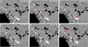 |
Fig. A.4. Evolution of the magnetic field BLOS from PHI observations in the region of interest near the large negative sunspot from 09:05 to 09:55 UT. Several magnetic polarities (labeled C1–C4) originate close to the sunspot. These polarities and the big negative N1-N2 show a motion towards each other over time. Four double-headed arrows are drawn in panel (f) such that the arrowheads touch two opposite-polarity patches. The same arrows are drawn on panels (a), (b), (c), and (e) for each of the C1–C4 patches. By comparing these panels with panel (f), it can be seen that the opposite polarities move closer to each other and magnetic flux convergence is increasing. |
A.1. EUI
The Extreme Ultraviolet Imager (EUI, Rochus et al. 2020) was running its high-resolution imager at 174 Å (HRIEUV) at a cadence of 10 s. The observations started at 09:00:07 UT and ended at 10:59:37 UT. From an Earth-based observer’s perspective, the observations started at 09:05:01 UT. The HRIEUV has a pixel scale of  which on 20 Oct 2023 corresponded to 146 km in the solar atmosphere. The HRIEUV FOV covered an area of 297 × 297 Mm (or 411″ × 411″ as seen from 1 AU). The HRIEUV 174 Å channel is dominated by emission from Fe IX and Fe X spectral lines. The HRIEUV 174 Å images that we show here were processed with wavelet-optimized whitening (WoW; Auchère et al. 2023) to enhance small-scale features.
A.2. PHI
The Polarimetric and Helioseismic Imager (PHI; Solanki et al. 2020) was running its high-resolution telescope (HRT; Gandorfer et al. 2018) at a cadence of 1 min. The observations started at 05:30:03 UT and ended at 11:29:09 UT. The HRT has a pixel scale of  which on 20 Oct 2023 corresponded to 148 km in the solar atmosphere. The HRT FOV covered an area of 228 × 228 Mm (or 316″ × 316″ as seen from 1 AU). The PHI data products are derived from Milne-Eddington inversions of spectro-polarimetric observations in the Fe I 6173 Å line. We estimate that the noise level in the level 2 BLOS line-of-sight magnetic field maps is about 10 G. This noise estimate was derived from the standard deviation in quiet regions in the data.
A.3. SST
At the Swedish 1-m Solar Telescope (SST, Scharmer et al. 2003), we acquired imaging spectroscopy data in the Hα line with the tunable filtergraph CRISP (Scharmer et al. 2008). The Hα line was sampled at 19 line positions with regular steps of 0.1 Å between ±0.9 Å offset from nominal line center. The time to complete one spectral scan was 8.9 s. Because the seeing was variable and at times of not acceptable quality, the data was recorded in trigger mode: the acquisition of a new spectral line scan was only triggered if the seeing quality was higher than a specific threshold. The seeing quality at the SST is measured by the adaptive optics system (Scharmer et al. 2024) in terms of the Fried parameter r0 (also see Scharmer et al. 2019). The trigger threshold was put to r0 ≥ 6 cm for the ground-layer seeing. The resulting 106 min time sequence has 511 time steps with variable interval. The average cadence is 12.5 s. There are three time gaps that are longer than 1 min (the longest 105 s). The Fried parameter varied between 3 and 15 cm (3−26 cm for the ground-layer seeing). The observations started at 09:05:03 UT. After the upgrade of the cameras in late 2022, the CRISP FOV is circular with a diameter of about 87″ and the pixel scale is  pixel−1 (32 km). The data was processed following the standard SST data reduction pipeline (de la Cruz Rodríguez et al. 2015; Löfdahl et al. 2021) which includes Multi-Object Multi-Frame Blind Deconvolution (MOMFBD, Van Noort et al. 2005) image restoration.
A.4. IRIS
The Interface Region Imaging Spectrograph (IRIS, De Pontieu et al. 2014) was running a very-large sparse 2-step raster program (OBSID 3420257611) with an exposure time of 4 s. The slit-jaw imager only acquired images in the SJI 1400 Å channel at a cadence of 10 s. The pixel scale of the SJI 1400 images is  (120 km) and the FOV about 166″ × 182″. IRIS observed between 09:06:17 and 10:54:00 UT.
A.5. SDO
From the Solar Dynamics Observatory (SDO, Pesnell et al. 2012), we use data from the Atmosphere Imaging Assembly (AIA, Lemen et al. 2012) and the Helioseismic Magnetic Imager (HMI, Scherrer et al. 2012) instruments for context and comparison. AIA observes the full solar disk at a cadence of 12 s in the EUV channels and at a cadence of 24 s in the 1600 Å and 1700 Å UV channels. The pixel size of AIA is  (434 km). HMI provides maps of the full disk photospheric magnetic field with a cadence of 45 s and a pixel size of
  (361 km). We aligned the SDO data to the SST observations using the methods in Solar Soft SSWIDL developed by Prof. R. Rutten1.
All Figures
|
Fig. 1. Outline of the areas covered by different instruments, drawn on a full-disc AIA 171 Å image. The diagram in the top right indicates the viewing angle (44°) and heliocentric distance (0.41 AU) of Solar Orbiter compared with SST, IRIS, and SDO, which all observe along the Earth-Sun viewing line. |
| In the text | |
|
Fig. 2. Observations from Solar Orbiter (reprojected to Earth’s view), SST, and IRIS showing a fibril singularity and a blow-out jet around 09:40 UT. The Solar Orbiter/PHI magnetogram (left panel) shows the sunspot’s moat flow, containing small-scale magnetic patches (see the attached animation). The black arrow in the SST panel indicates the chromospheric material ejected from the peeling of the arch filament system. The white box shows the field of view of Fig. 3. This figure is associated with an online animation (PHI+SST+EUI+IRIS_2023-10-20_fullfov.mp4). |
| In the text | |
|
Fig. 3. Zoomed-in view of the area outlined by the white box in Fig. 2. A strong moat flow is observed near the jet base and is marked with a black arrow in panel a. Four main positive- and negative-polarity patches are labelled as P1, P2, N1, and N2 respectively. The blow-out jet in the coronal EUV 174 Å image, associated with a chromospheric surge in Hα, is indicated with grey arrow in panels b and c. Fibrils and the ‘X’-shaped saddle-point structure are marked in the Hα image. A flaring loop associated with the chromospheric fibril singularity is shown in EUI and Hα. Potential-field extrapolations on the PHI magnetogram are shown in panels d–e. In panel d, the yellow arrow indicates the jet base, which consists of a fan-spine configuration with a null point and associated outer spine towards the west (black arrow). A zoomed-in version is shown in panel e, where several inverted ‘Y’ structures are shown from the weak magnetic corridor between N1 and N2. |
| In the text | |
|
Fig. 4. Intensity light curves at the flaring loop location in different AIA channels. The curves display a flare-like evolution, with a rapid heating phase that is most pronounced in the hotter channels, and a cooling phase after the peak around 09:46 UT that is slower in the cooler channels. The position of the box used to compute the intensity is indicated in Fig. A.1. |
| In the text | |
|
Fig. 5. Schematic representation of the observations. The two colliding regions of negative polarity are overlaid with chromospheric fibrils, shown in brown. The flaring loop along the fibril singularity is indicated by a curved orange arrow pointing left. The fibril singularity line is shown in magenta, with a saddle point at one end indicated in green. A saddle point is shown at the boundary between fan surfaces and the fibril singularity. Multiple inverted ‘Y’ structures along the fibril singularity are illustrated with parallel black colour behind the main null-point structure at the jet base. |
| In the text | |
|
Fig. A.1. Blow-out jet at the time around maximum extent in IRIS SJI 1400 Å, AIA 171 Å, and EUI/HRIEUV 174 Å. The rectangular white box highlighted in the middle panel was used to compute the intensity variation presented in Fig. 4. The EUI image is shown without reprojection to the Earth viewing direction. An animation of this figure is available in the online material (AIA171+EUI+IRIS_2023-10-20_jet.mp4). |
| In the text | |
|
Fig. A.2. Reconnection regions and rapid motion of photospheric magnetic fields close to the sunspot. In Hα blue wing (left panel) the reconnection sites are outlined with blue contours, where enhanced Hα wing emission mark the location of Ellerman Bombs. The intensity at these locations is 1.45 times the intensity of the reference quiet Sun spectrum. The middle panel shows the cotemporal and aligned PHI BLOS map. Yellow circles mark the locations of these reconnection points. The right panel shows, at each pixel, the extremum of BLOS over 1 h before the onset of the jet generated from the original PHI data. Red contours mark pixels that have |BLOS|> 100 G for both polarities during the 1 h sequence. |
| In the text | |
|
Fig. A.3. Recurrent blow-out jets and flaring loop along the fibril singularity in EUI/HRIEUV 174 Å (top and middle row) and SST/Hα (bottom row) observations. These activities along the fibril singularity occur at three different times along the whole duration of the coordinated observations (see the animation associated with Fig. 2) as shown in the middle row. Sometimes these are closely associated with the blow-out jets. Our main event is for the Jet 1 and flaring loop 1 around 09:40 UT. |
| In the text | |
|
Fig. A.4. Evolution of the magnetic field BLOS from PHI observations in the region of interest near the large negative sunspot from 09:05 to 09:55 UT. Several magnetic polarities (labeled C1–C4) originate close to the sunspot. These polarities and the big negative N1-N2 show a motion towards each other over time. Four double-headed arrows are drawn in panel (f) such that the arrowheads touch two opposite-polarity patches. The same arrows are drawn on panels (a), (b), (c), and (e) for each of the C1–C4 patches. By comparing these panels with panel (f), it can be seen that the opposite polarities move closer to each other and magnetic flux convergence is increasing. |
| In the text | |
Current usage metrics show cumulative count of Article Views (full-text article views including HTML views, PDF and ePub downloads, according to the available data) and Abstracts Views on Vision4Press platform.
Data correspond to usage on the plateform after 2015. The current usage metrics is available 48-96 hours after online publication and is updated daily on week days.
Initial download of the metrics may take a while.