| Issue |
A&A
Volume 706, February 2026
|
|
|---|---|---|
| Article Number | A97 | |
| Number of page(s) | 15 | |
| Section | Stellar atmospheres | |
| DOI | https://doi.org/10.1051/0004-6361/202557298 | |
| Published online | 03 February 2026 | |
Hydrodynamical mass-loss rates for very massive stars
I. Investigating the wind kink
1
Armagh Observatory and Planetarium,
College Hill,
Armagh
BT61 9DG,
Northern Ireland,
UK
2
Zentrum für Astronomie der Universität Heidelberg, Astronomisches Rechen-Institut,
Mönchhofstr. 12-14,
69120
Heidelberg,
Germany
★ Corresponding author: This email address is being protected from spambots. You need JavaScript enabled to view it.
Received:
17
September
2025
Accepted:
14
December
2025
Abstract
Radiation-driven winds are ubiquitous in massive stars, but in very massive stars (VMSs), mass loss dominates their evolution, chemical yields, and ultimate fate. Theoretical predictions have often relied on extrapolations of O-star prescriptions, likely underestimating true VMS mass-loss rates. In the first of a series of papers on VMS wind properties, we investigate a feature predicted by Monte Carlo (MC) simulations: a mass-loss ‘kink’ or upturn where the single-scattering limit is breached and winds transition from optically thin to optically thick. We calculated hydrodynamically consistent wind-atmosphere models in non-local thermodynamic equilibrium using the POWRHD code, with a grid spanning 40-135 M⊙ and 12-50kK at fixed log(L*/L⊙) = 6.0 and solar-like metallicity with Z = 0.02. Our models confirm the existence of the kink, where the wind optical depth crosses unity and spectral morphology shifts from O-star to WNh types. The predicted location of the kink coincides with the transition stars in the Galactic Arches Cluster and reproduces the model-independent transition mass-loss rate of log(Ṁtrans) ≈ −5.16 from Vink & Gräfener (2012). For the first time, we locate the kink at Γe ≈ 0.43 (M* ≈ 60 M⊙) without relying on uncertain stellar masses. Above the kink, mass-loss rates scale much more steeply with decreasing mass (slope ~10), in qualitative agreement with MC predictions. We additionally identified two bistability jumps in the mass loss driven by Fe ionisation shifts: the first is from Fe IV → Fe III near 25 kK, and the second is from Fe III → Fe II near 15 kK. Our models thus provide the first comprehensive confirmation of the VMS mass-loss kink while establishing a mass-loss relation with complex mass and temperature dependencies with consequences for stellar evolution, chemical yields, and the black hole mass spectrum.
Key words: stars: atmospheres / stars: massive / stars: mass-loss / stars: winds, outflows / stars: Wolf-Rayet
© The Authors 2026
 Open Access article, published by EDP Sciences, under the terms of the Creative Commons Attribution License (https://creativecommons.org/licenses/by/4.0), which permits unrestricted use, distribution, and reproduction in any medium, provided the original work is properly cited.
This article is published in open access under the Subscribe to Open model. This email address is being protected from spambots. You need JavaScript enabled to view it. to support open access publication.
1 Introduction
Winds from massive O-type stars in the range of 20-60 M⊙ are a key ingredient in stellar evolutionary models, shaping both their structure and their final fate. However, for the most massive stars in the Universe with initial masses above 100 M⊙ - the so-called very massive stars (VMSs) - mass loss is not merely important: It is the dominant factor that determines their evolution and ultimate fate (Hirschi 2015; Köhler et al. 2015).
O-star winds have long been described by the optically thin line-driving theory of Lucy & Solomon (1970) and Castor et al. (1975, hereafter CAK). Evolutionary models for VMSs have traditionally extrapolated these prescriptions into higher masses. However, such extrapolations likely underestimate the true VMS mass-loss rates. Vink et al. (2011) using Monte Carlo (MC) simulations predicted an upturn or a ‘kink’ in the mass-loss-luminosity relation, associated with the Eddington parameter Γ ∝ L/M. This kink suggests that winds strengthen dramatically and become optically thick; that is, the wind optical depth, τF, crosses unity, as stars approach the Eddington limit.
Concurrently with these VMS wind predictions, the widely assumed stellar upper-mass limit of 100-150 M⊙ (Weidner & Kroupa 2004; Figer 2005; Oey & Clarke 2005) was revised to ~200-300 M⊙ (Crowther et al. 2010; Bestenlehner et al. 2011; Martins 2015; Brands et al. 2022; Kalari et al. 2022). These values, however, are based on present-day masses extrapolated to the zero-age main sequence (ZAMS) using O-star rates, and may thus be underestimated. If VMS mass loss is indeed stronger than CAK extrapolations suggest, the intrinsic upper-mass limit may extend significantly higher - perhaps up to 1000 M⊙ (Vink 2018; Sabhahit et al. 2022; Higgins et al. 2022). A closely related issue concerns the formation of VMSs (Krumholz 2015) and the upper-mass limit, which may be regulated by the strength of stellar winds in environments of different metallicity.
In the local Universe, the hydrogen-rich class of Wolf-Rayet stars of the nitrogen (N) sequence (WNh stars) in young (~1-2 Myr) massive clusters, which exhibit strong He II emission, are our best candidates for VMSs (Massey & Hunter 1998; de Koter et al. 1998; Martins et al. 2008; Crowther et al. 2016; Wofford et al. 2014; Upadhyaya et al. 2024). Such VMSs are not only key to stellar evolution theory but also to astrophysical environments, since they may drive the chemical enrichment of globular clusters (Vink 2018; Higgins et al. 2023, 2025; Gieles et al. 2025) and also provide crucial feedback at high redshift (Senchyna et al. 2024; Vink 2023; Charbonnel et al. 2023; Cameron et al. 2023; Isobe et al. 2023; Topping et al. 2024; Curti et al. 2025; Ji et al. 2025). Predicting their wind yields and final masses requires reliable mass-loss prescriptions, especially across the transition from optically thin (τF < 1) O-star winds to optically thick (τF > 1) WNh winds (Vink & Gräfener 2012).
The Vink et al. (2011) kink approximately coincides with the wind efficiency parameter η = Ṁv∞c/L approaching unity. Above this threshold, the predicted mass-loss scaling with Γ steepens from approximately two to about five, far stronger than a CAK-style extrapolation. While CMFGEN analyses from the VLT-FLAMES Tarantula Survey (Bestenlehner et al. 2014) provide empirical support, several studies still neglect the η ≈ τF ≈ 1 criterion emphasised by Vink & Gräfener (2012).
Given the upturn or kink predicted by the MC simulations, wind calculations using a different method and code are important to independently verify the MC results, which motivates new predictions of VMS mass-loss rates both below and above the potential upturn or kink. Here we present new computations with the hydrodynamically consistent branch of the Postdam Wolf-Rayet (PoWR) code (Sander et al. 2017), as recently applied to the study of late-type WNh stars (Lefever et al. 2025) and some of the most massive stars in the R136 cluster in the Large Magellanic Cloud (LMC) (Sabhahit et al. 2025). These kinds of hydro-models are also ideal tools to study the transition from absorption-line dominated O-star spectra to emission-line dominated WNh spectra as the objects approach the Eddington limit. Along this transition, in particular, the equivalent width of the Wolf-Rayet (WR) He II emission feature increases (see Vink et al. 2011; Crowther & Walborn 2011).
The paper is organised as follows: in Sect. 2, we detail the basics of our hydrodynamical wind-atmosphere models and the necessary inputs and outputs. In Sects. 3 and 4, we present the radiative acceleration and mass-loss properties of VMSs, discussing the mass-loss kink feature and bistable behaviour at cooler temperatures. We further test our mass-loss predictions against the transition mass-loss rate in the Arches Cluster. A brief comparison to previous VMS wind investigations is presented in Sect. 5, and we conclude in Sect. 6.
2 PoWRHD atmosphere models
We utilised the hydrodynamical branch of the non-local thermodynamic equilibrium (non-LTE) stellar atmospheric code PoWR (Gräfener et al. 2002; Hamann & Gräfener 2003; Gräfener & Hamann 2005, 2008; Sander 2015; Sander et al. 2015, 2017) to build our model atmosphere grid. PoWR models a onedimensional, spherically symmetric, expanding atmosphere by solving the equations of radiative transfer, statistical and thermal equilibrium, and continuity. The atmosphere computational framework has long relied on the Accelerated Lambda Operator iteration (for details, see Hamann 1985, 1986) to solve these fully coupled non-linear equations across both spatial and frequency domains. Radiative transfer calculations are performed using the co-moving frame approach, in which the opacity and emissivity profile functions become isotropic (Mihalas et al. 1975). The code takes relevant stellar and wind parameters as inputs and computes the emergent synthetic spectra. The input stellar parameters include luminosity, temperature (or radius), logg (or mass), and chemical abundances (for a detailed input parameters, see Sect. 2.1). The wind parameters are specified by the mass-loss rate, Ṁ, and the velocity stratification, v(r), which is typically prescribed using a standard β-type velocity law of the form v(r) ~ (1 - R*/r)β.
The fundamental advance and novelty of the PoWRHD models over the base code stems from solving the stationary hydrodynamic equation of motion (cf. Eq. (1)). The code balances the time-independent advective acceleration term (υdυ/dr), against the various forces in the wind-atmosphere, such as gravity and the gas and radiation pressure gradients at each atmospheric layer, thereby integrating hydrodynamics into the overall iterative procedure of the atmosphere code. By solving the wind hydrodynamics, the models gain predictive power, as the mass-loss rate and the wind velocity stratification are no longer prescribed inputs. These quantities instead emerge as predicted outputs, calculated self-consistently from the atmospheric force balance at each iteration step.
Such next-generation hydrodynamically consistent atmosphere models therefore achieve what earlier codes could not: they simultaneously derive consistent wind structure and mass loss, and generate synthetic spectra through unified non-LTE atmosphere-hydrodynamics calculations, enabling empirical determination of fundamental stellar and wind parameters (see e.g. Sander et al. 2017; Sabhahit et al. 2025). The numerical implementation details and general input specifications are documented in detail in Sander (2015); Sander et al. (2017, 2020). Below, we briefly summarise the required inputs to build our model grid and the relevant outputs.
2.1 Key input parameters
In this work, we isolated the effects of stellar mass and inner boundary temperature on VMS wind properties. While a comprehensive parameter space exploration and theoretical massloss predictions for the most-massive WNh stars based on PoWRHD models will follow in a forthcoming work, the present study maintains all parameters except mass and temperature at the fixed values detailed below.
We fixed the luminosity to a constant value of log(L*/L⊙) = 6.0 throughout our grid. The inner boundary radius, R*, of our models is defined at a specific Rosseland continuum optical depth, τR,cont, of 20. The effective temperature, T*, at the inner boundary is varied between 12-50 kK, primarily encompassing the temperature range characteristic of observed WNh stars and luminous blue variables (LBVs) at this luminosity. The stellar mass range extended from approximately 40-135 M⊙, with the precise range depending on T*1. The outer boundary was set to Rout = 1000 R*.
For the chemical abundances, we adopted ZAMS values following solar-scaled patterns from Grevesse & Sauval (1998), with a total metal mass fraction of Z = 0.02 (Appendix B details the mass fraction breakdown for individual elements, along with levels and lines per ion). The hydrogen (H) mass fraction was fixed at X = 0.7, while helium (He) followed from the unity constraint X + Y + Z = 1.
Density inhomogeneities - ubiquitous in massive star winds - were incorporated through the micro-clumping formalism of Hillier et al. (2003), with the clumping onset occurring at a specified Rosseland optical depth (see Sander et al. 2017, for the implementation). The clumping factor, Dcl, was increased from unity (smooth wind) to an asymptotic value, Dcl,∞ = 10, with the onset at Rosseland optical depth τR = 0.1. This choice of onset is motivated by multi-wavelength spectral fits to archetypal VMSs in the Tarantula Nebula, specifically R136a1 (WN5h) and the binary system R144 (WN5/6h+WN6/7h) using PoWRHD models (Sabhahit et al. 2025). Turbulent pressure contributions were included through adoption of a radially constant turbulent velocity υturb = 70km s−1. Such high values are motivated from time-dependent, 2D simulations of massive O-star atmospheres, where substantial photospheric turbulence of the order 30-100 km s−1 is expected to originate from the hot iron (Fe) bump (Debnath et al. 2024).
2.2 Output quantities
The PoWRHD models enforce the stationary hydrodynamic equation of motion throughout the atmosphere:
 (1)
(1)
where P(r) is the combined gas and turbulent pressure, while ρ(r) and υ(r) denote the mass density and velocity stratifications which are linked to the mass-loss rate Ṁ through the continuity equation: Ṁ = 4πr2ρ(r)υ(r). The total radiative acceleration arad(r), arising from momentum transfer on transition lines, scattering, and other continuum processes, fundamentally couples the hydrodynamic equation to the radiation field and population numbers.
Equation (1) fundamentally represents the force balance equation, with the advective acceleration term on the left-hand side counterbalanced by the cumulative atmospheric forces on the right - gravity and the gradients of gas, radiation, and turbulent pressure. The apparent simplicity of Eq. (1) is however misleading. The complexity lies masked within the radiative acceleration term arad(r), given by
 (2)
(2)
where ϗF(r) and F(r) represent the flux-weighted mean opacity and total flux at radius r, respectively. The quantity ϗF(r) cannot be determined locally; it must instead incorporate the detailed frequency-dependent opacity, which depends on radiation and velocity fields, along with ionisation and excitation states of absorbing ions throughout the atmosphere. Such complexity demands a brute-force, iterative global integration to achieve self-consistent hydrodynamic atmosphere models.
The flux-weighted mean opacity calculation is however essential because it accounts for Doppler effects in the expanding wind and ensures accurate radiative acceleration through conservation of the flux integral in Eq. (2). Unlike the classical Thomson acceleration - well constrained at model initialisation, particularly when stellar temperatures are high enough for complete H and He ionisation - the total radiative acceleration is calculated iteratively. The radial stratification of this total radiative acceleration from converged models is examined in Sect. 3.
Using the continuity equation in Eq. (1) and rearranging the hydrodynamic equation such that all terms containing the velocity gradient are grouped together on one side, we can show that the hydrodynamic equation features a critical point at radius Rcrit (see derivation in Sander et al. 2017). The critical point in our model occurs where the flow velocity equals the isothermal sound speed corrected for turbulent velocity2, so that the critical radius Rcrit roughly coincides with the sonic point radius Rsonic. Each hydrodynamic update recalculates the velocity stratification throughout the atmosphere via inward and outward integration from Rcrit. We therefore predict the complete velocity stratification υ(r), including the terminal velocity at the outer boundary: υ∞ = υ(r = Rout). Mass-loss rate updates preserve the inner boundary condition to maintain the specified TR,cont.
From the predicted Ṁ and υ∞, the wind efficiency parameter is given by:
 (3)
(3)
The parameter η quantifies the ratio of wind momentum to available photon momentum. For powerful winds characteristic of WNh and classical WR stars, where multiple photon scattering becomes significant, η can easily exceed the single-scattering limit of unity.
Another important wind-related quantity outputted by our models is the wind optical depth, specifically, the flux-weighted mean wind optical depth at the sonic point. It is calculated by integrating the product of flux-weighted mean opacity and density inward from the outer boundary:
 (4)
(4)
Since we obtain a detailed solution to the radiative transfer problem, we predict the flux-weighted mean opacity and therefore output the wind optical depth.
Finally, converged models generate emergent synthetic spectra through formal integration in the observer’s frame, incorporating relevant broadening mechanisms. We additionally computed ionising photon fluxes (photons per second) by integrating the emergent spectrum shortward of relevant continuum edges, for instance, the Lyman continuum edge yields the H-ionising flux. These predicted quantities from our models are detailed below, while Appendix B provides a comprehensive table of wind-related outputs from our PoWRHD models.
3 Radiative acceleration
A major advance in our understanding of hot-star winds over recent decades has been recognising the importance of proximity to the Eddington limit (Gräfener & Hamann 2008; Vink et al. 2011; Sander & Vink 2020). Yet predicting a priori how metal-licity and other stellar parameters affect VMS winds remains challenging, which is precisely why detailed radiative transfer calculations, such as those performed here are essential.
Nevertheless, we can infer qualitative trends to first order from the force balance in stellar winds (see Sabhahit et al. 2025, for a didactic study). The balance of relevant forces in massive star winds is characterised by the total radiative Eddington parameter, defined as the ratio of total radiative acceleration to gravity:
 (5)
(5)
where the radial variation in total Γrad primarily reflects changes in the flux-weighted mean opacity. The luminosity L(r) technically varies with radius r, since a fraction of the photon energy is used to lift the material out of the stellar gravitational potential and to accelerate it to a certain kinetic energy. However, even for powerful WR-type winds, the approximation, L(r) ≈ L*, is justified, as the deviations typically remain below ~5% (e.g. Sander et al. 2020).
Figure 1 illustrates the radial variation of total Γrad for a representative very massive star model with M* = 105 M⊙ and T* = 35 kK. We decompose this into contributions from boundbound line transitions, Γlines, and continuum processes, Γcont, which includes free-free (ff) and bound-free (bf) continuum terms plus classical electron (Thomson) scattering Γe:
 (6)
(6)
The classical Γe provides a useful measure of the star’s proximity to the Eddington limit, maintaining near-constancy throughout the atmosphere (solid magenta in Fig. 1). The classical Γe is given by:
 (7)
(7)
where σe denotes the electron scattering opacity. For sufficiently high temperatures capable of fully ionising H and He (electron temperatures above approximately 10 and 50kK, respectively), the electron scattering opacity remains essentially constant. While this generally holds throughout the inner, sub-critical region of the atmosphere where such conditions are realised, the low-temperature sequences in our grid can show a slight decrease in Γe near the critical point. Therefore, the Γe values reported in the subsequent sections are averages taken within the sub-critical region.
Two important conclusions emerge from examining the continuum component. First, the true continuum contribution from ff+bf transitions remains vanishingly small relative to electron scattering, evident from the minimal difference between Γcont and Γe terms. Second, although the continuum component dominates total Γrad in the sub-critical inner atmosphere - accounting for over 70% of the total - it cannot launch the wind. Wind launching requires Γrad to exceed unity. As the figure demonstrates, continuum processes alone provide insufficient acceleration to overcome gravity; line transitions are essential for wind initiation.
The dominant contributors to line acceleration in the sub-critical region where mass-loss rates are established are line opacities of FeII-FeVII (depending on T*). Immediately below the critical point, Fe provides the necessary acceleration to increase total Γrad to unity. Despite its relatively low abundance compared to other surface metals, the efficiency of Fe wind driving is due to the spectral coincidence between millions of Fe transitions and the ultraviolet peak characteristic of hot stellar photospheres.
Beyond the critical point, line opacities from several additional elements become important, extending beyond the CNO group. Notable contributors to outer-wind driving include Si, P, S , Cl, and Ar (see also Vink et al. 1999; Sander et al. 2017). Contributions from Si, P, and S are significant in our WNh models, as well as in the B hypergiant models applied to ζ1 Sco by Bernini-Peron et al. (2025) and in late-WNh models from Lefever et al. (2025). This contrasts with pure-He classical WR winds, where these contributions are negligible (Sander et al. 2020), meaning the contribution of Si, P, and S is generally important for stars on or rightward (cooler) of the ZAMS.
Iron’s pivotal role in inner-wind driving is further demonstrated by its absolute and relative contributions to Γlines. Figure 2 presents a stacked plot comparing contributions from various components to total Γrad and Γlines at the critical point as a function of stellar mass for our T* = 35 kK temperature sequence. In the top sub-panel, as stellar mass decreases, the Γe component at the critical point increases monotonically while line transition contributions decrease. The Fe contribution remains roughly constant at approximately 40% across most of the parameter space before dropping to roughly 20% at the lowest masses. In the lowest-mass model, despite Fe contributing only 20% of total Γrad, wind launching remains almost entirely Fe-driven. In the bottom sub-panel, Fe contributes more than half of the total line acceleration and remains approximately constant with mass. As we demonstrate in Sect. 4.3, insufficient Fe driving can lead to steep drops in the mass-loss rate in certain temperature and mass regimes.
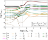 |
Fig. 1 Total radiative acceleration and its contributions from continuum processes and line transitions. Decomposition of the total radiative acceleration (solid black) into continuum (dashed green) and line (dashed red) components along with individual contributions from constituent elements in the atmosphere (coloured lines with symbols, see legend). Each of these element contributions consists of the sum of their line and continuum accelerations. All accelerations are normalised to gravity. The dotted and dashed vertical grey lines mark the sonic and critical points, Rsonic and Rcrit, respectively. The model stellar parameters are log(L*/L⊙) = 6.0, M* = 105 M⊙, T* = 35kK, X = 0.7, and Z = 0.02. |
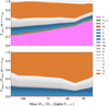 |
Fig. 2 Contributions from electron scattering, free-free and bound-free continuum transitions, and line transitions of individual elements at the critical point, shown as a function of mass. The contributions are normalised to gravity and expressed as Eddington parameters. Top : absolute contributions from different opacity sources. Bottom : relative line contributions from different elements. The model sequence corresponds to a temperature of T* = 35 kK. |
4 Winds of VMSs
4.1 Testing against the transition mass-loss rate
Determining mass-loss rates for hot, massive stars presents significant challenges, with several complementary approaches available (see Vink 2022, for a recent review). Empirical determinations typically involve fitting observed wind-sensitive spectral lines such as Hα or UV diagnostics using non-LTE expanding atmosphere models. In this iterative process, stellar and wind parameters are varied until optimal spectral fits are achieved, from which one can infer the best-fit empirical mass-loss rates. Alternatively, we can predict theoretical massloss rates using analytical models based on CAK theory and its subsequent improvements accounting for complex line-lists and finite-disc effects (Castor et al. 1975; Friend & Abbott 1986; Pauldrach et al. 1986), semi-analytical approaches such as MC simulations (e.g. Lucy & Abbott 1993; Vink et al. 2001; Müller & Vink 2008), or hydrodynamically consistent stellar windatmosphere models (Gräfener & Hamann 2005; Sander & Vink 2020), such as those investigated here.
Each approach comes with their own inherent limitations. Optical wind-line diagnostics - mainly recombination lines - are inherently model-dependent and strongly sensitive to assumptions about wind clumping in the underlying atmosphere models. As the adopted clumping factor increases, empirically derived rates systematically decrease (Hamann & Koesterke 1998). Furthermore, degeneracies between stellar and wind parameters can make it impossible to uniquely determine best-fit values. Theoretical predictions also suffer from clumping uncertainties, with predicted mass-loss rates depending on clumping assumptions near the critical point (Gräfener & Hamann 2005; Muijres et al. 2011; Sabhahit et al. 2025; Bernini-Peron et al. 2025).
To address these challenges, Vink & Gräfener (2012) developed the concept of the transition mass-loss rate. The underlying idea is straightforward: at the observed spectral morphological transition from absorption-dominated O star spectra to emissionline-dominated WNh star winds (as seen in the Hβ transition described by Crowther & Walborn 2011), the wind optical depth crosses approximately unity.
Building on the hydrodynamic equation of motion, Vink & Gräfener (2012) derived an analytical formula linking wind efficiency and optical depth to describe this spectral transition condition:
 (8)
(8)
Through extensive testing across a range of stellar parameters, Vink & Gräfener (2012) found that the factor f depends primarily on the terminal-to-escape velocity ratio υ∞/υesc and on the velocity-law exponent β. For Galactic metallicity and υ∞/υesc = 2.5, they obtained f ≈ 0.6, assuming a β-type velocity law with relatively large values of β ≈ 1.5, typical of very massive-star winds (Vink et al. 2011; Sabhahit et al. 2025). The dependence of f on the υ∞/υesc ratio was parametrised in Sabhahit et al. (2023) as  (for an analytical derivation, see Gräfener et al. 2017). Although clumping assumptions can in principle influence the υ∞/υesc ratio, and therefore the value of f, the impact is small because f approaches a plateau once the υ∞/υesc ratio is sufficiently high.
This means the transition from optically thin O-star winds to optically thick WNh-star winds approximately coincides with both the wind efficiency parameter η and τF(rsonic) crossing order unity. Beyond this transition, Vink et al. (2011) discovered a steep upturn in predicted mass loss with the classical Eddington parameter, creating the characteristic kink in the Ṁ(Γe) relation discussed in the introduction.
Vink & Gräfener (2012) rearranged Eq. (8) to formulate the concept of the transition mass-loss rate:
 (9)
(9)
As Eq. (9) reveals, the transition mass-loss rate is essentially a luminosity estimate expressed in mass-loss units. The luminosity and terminal velocity of transition objects can be determined with greater accuracy than empirical measures of the mass-loss rate as the latter depend on model specifics such as clumping assumptions. Uncertainties in f typically fall within the error bars of luminosity measurements. This gives the transition massloss rate a crucial advantage: it is both accurate and significantly less model-dependent than traditional estimates. However, this accuracy applies specifically to the transition region between O and WNh stars, not beyond it.
Consider the Arches Cluster which hosts several O stars and WNh stars. The transition objects - whose spectral morphology bridges absorption-dominated O stars and emissionline-dominated WNh stars - have luminosities and terminal velocities of approximately log(L*/L⊙) ≈ 6.06(±0.1) and υ∞ ≈ 2000(±400) km s−1 (Martins et al. 2008). Applying Eq. (9) yields a transition mass-loss rate of log(Ṁtrans) ≈ −5.16 (Vink & Gräfener 2012; Sabhahit et al. 2022).
Given the accurate and model-independent nature of this approach, any credible mass-loss prescription - whether empirical or theoretical - should reproduce this rate at the luminosity and temperature of the transition stars. While agreement at the transition does not guarantee accuracy elsewhere, it provides an essential first-order sanity check: if a prescription fails to match the transition mass-loss rate, we can confidently consider it inaccurate within this regime.
Figure 3 shows how our PoWRHD models perform against the Arches transition mass-loss rate. We compare our predicted rates for the T* = 35 kK model sequence with the transition massloss rate of log(Ṁtrans) ≈ −5.16. The T* = 35 kK sequence is selected such that its surface temperatures, defined at Rosseland optical depth τR = 2/3 as Teff(τR = 2/3), is close to the observed Teff ≈ 33.4kK of the transition objects. Our PoWRHD models successfully reproduce the transition mass-loss rate at stellar parameters corresponding to the Arches transition objects.
We also compare the Arches transition mass-loss rate with the widely used Vink et al. (2000) mass-loss predictions. As shown in Figure 3 - and as already noted by Vink & Gräfener (2012) - the Vink et al. (2000) rates agree well with the transition mass-loss rates for the relevant stellar parameters. However, the Vink et al. (2000) rates diverge from our predictions both above and below the transition point. This deviation becomes particularly pronounced at lower masses or higher Γe, where our predicted mass loss exhibits a steeper scaling with mass and consequently with Γe above the transition. The presence of a kink in the mass-loss rate agrees with the results of Vink et al. (2011).
Our models predict a terminal velocity of 1500 km s−1 at the transition, approximately 500 km s−1 lower than observed in Arches transition objects. However, terminal velocity predictions are notoriously sensitive to outer wind conditions, including temperature stratification and clumping, both of which remain uncertain. We can achieve better agreement by increasing outerwind clumping, which enhances outer-wind driving and boosts terminal velocity. Indeed, such an increase in outer-wind clumping was required to reproduce the UV+optical spectra of R136a1 and R144 using hydrodynamical models (Sabhahit et al. 2025).
Figure 3 also compares our predicted wind efficiency parameter and optical depth with transition values from Vink & Gräfener (2012). Additionally, Figs. 4 and 5 display synthetic optical and UV spectra for the T* = 35 kK model sequence, highlighting crucial wind-sensitive recombination and P-Cygni lines. At the point where our models match the Arches transition mass-loss rate, we find η ≈ 0.45. This value falls below the Vink & Gräfener (2012) transition value of η ≈ 0.6, likely reflecting our underestimated terminal velocities. The wind optical depth crosses unity precisely at the transition, coinciding with the spectral morphological change where Hβ shifts from absorption to emission. We observe similar behaviour in Hγ, while Hα transitions from absorption to emission at higher masses (i.e, lower Γe) compared to other Balmer lines. In contrast, He II λ4686 remains in emission throughout the sequence, strengthening as mass decreases. In the UV, one can see the expected sensitivity of the the CIV λ1550 and SiIV λ1400 resonance doublets to the terminal velocity in our model. Additional features also appear in the UV, for example around λ1470, which is an iron feature that strengthens as the winds become optically thick.
Finally, we can estimate the stellar mass required in our hydrodynamic models to match the transition mass-loss rate. We intend to closely match the (averaged) observed stellar luminosity and surface temperature of the transition object in the Arches. To this end, we interpolate between our model sequences to precisely match the observed Teff(τR = 2/3) ≈ 33.4 kK (Martins et al. 2008). We find that M* ≈ 60 M⊙ (corresponding to Γe ≈ 0.43) and T* ≈ 38.2 kK is required to match the transition. This M* ≈ 60 M⊙ coincides with the kink location in our models and agrees well with predictions from Sabhahit et al. (2022) for the location of the kink in Γe-space.
To summarise our findings: our PoWRHD models successfully reproduce the transition mass-loss rate in the Arches Cluster, confirm the prediction of a mass-loss kink above the transition, and capture the morphological change in Hβ from absorption to emission as the wind optical depth crosses unity. While our model-predicted wind efficiency at the transition (η ≈ 0.45) is lower than Vink & Gräfener (2012) predicted η ≈ 0.6, this discrepancy likely stems from our underestimated terminal velocities. Overall, these results provide strong validation of our hydro-predicted mass-loss rate and its ability to capture the essential physics of the O to WNh star morphology transition.
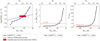 |
Fig. 3 Testing the PoWRHD model predictions against the transition mass-loss rate in the Arches Cluster. Left : predicted mass-loss rates versus stellar mass from PoWRHD models for the T* = 35 kK sequence (solid black) and from Vink et al. (2000) (dotted blue), compared to the transition mass-loss rate of log(M) ≈ −5.16 in the Arches (horizontal red line) from Vink & Gräfener (2012). The PoWRHD models are computed with fixed log(L*/L⊙) = 6.0, X = 0.7, and Z = 0.02, roughly matching the observed properties of the Arches transition objects (Martins et al. 2008). The T* = 35 kK sequence shown has surface temperatures close to the observed Teff(τR = 2/3) ≈ 33.4 kK of the transition objects. The stellar masses of the transition objects span ~55—75 M⊙ corresponding to their averaged luminosity and temperature. Middle : predicted wind efficiency parameter versus mass compared to the transition value η ≈ 0.6 (dashed red) from Vink & Gräfener (2012). Right : predicted wind optical depth versus mass compared to the transition value τF(rsonic) ≈ 1 (dashed red) from Vink & Gräfener (2012). |
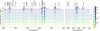 |
Fig. 4 Synthetic spectra showing relevant wind lines in the optical for the T* = 35 kK model sequence presented in Fig. 3. The spectra are colour-coded based on the stellar mass. |
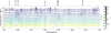 |
Fig. 5 Synthetic spectra showing relevant wind lines in the UV for the T* = 35 kK model sequence presented in Fig. 3. The spectra are colour-coded based on the stellar mass. |
4.2 Wind properties: Ṁ, υ∞,η, and τF(rsonic)
Figure 6 presents relevant wind parameters, including massloss rates and terminal wind velocities, as functions of stellar mass, with temperature sequences colour-coded by T*. Across all temperature sequences, we observe a consistent fundamental trend: mass-loss rates increase systematically towards lower stellar masses when other parameters remain fixed. This behaviour reflects the underlying physics: For fixed luminosity and composition, decreasing the stellar mass decreases the gravitational force in the wind and drives up the total Γrad in the sub-critical region (r < Rcrit), directly boosting mass-loss rates (cf. Castor et al. 1975; Lamers & Cassinelli 1999; Vink et al. 2001; Sander & Vink 2020; Sabhahit et al. 2025).
Terminal velocities follow a complementary pattern, generally decreasing with decreasing mass (cf. Castor et al. 1975; Friend & Abbott 1986), although the behaviour can be nonmonotonic sometimes (see e.g. the sequence in Lefever et al. 2025; Bernini-Peron et al. 2025). To first order, an increase in the total Γrad in the sub-critical regime (r < Rcrit) drives a higher mass loss but produces denser, slower winds. Conversely, increased Γrad in the supercritical region (r > Rcrit) accelerates winds to higher velocities without affecting mass-loss rates (see also Vink et al. 2001; Sander & Vink 2020).
More intriguing are the temperature-dependent variations in these scaling relations. Hotter models with T* ≳ 30 kK reveal a distinctive upturn - a characteristic kink - in the log Ṁ-log M (and therefore also the log Ṁ - log Γe) relation. The scaling behaviour transitions from the shallow slope of ~ 1.5-3 at higher masses (lower Γe) to a dramatically steeper slope of ~10 at lower masses (higher Γe). This behaviour qualitatively matches the MC predictions of Vink et al. (2011) and aligns with empirical evidence of such a kink in the 30 Doradus cluster reported by Bestenlehner et al. (2014).
In contrast, for the cooler models with T* ≲ 25 kK, their log Ṁ - log M relations maintain consistently steep slopes throughout our parameter range, showing no pronounced kink behaviour. Particularly notable are the T* = 25 and 15 kK sequences, which maintain distinctly steep slopes across the entire mass range.
Terminal velocity behaviour further distinguishes hot and cool regimes. Hotter models show terminal velocities that generally decline with decreasing mass, while cooler models exhibit weak mass dependence, remaining nearly constant at ~500 km s−1. Similarly low velocities were also obtained in the late WNh models of Lefever et al. (2025).
Both wind efficiency parameters and optical depths increase monotonically with decreasing mass across all temperatures. At kink locations in hotter models, wind efficiency reaches approximately 0.4-0.45 - notably lower than the Vink & Gräfener (2012) transition value of η ≈ 0.6, likely reflecting our underestimated terminal velocities. On the other hand, wind optical depths cross unity precisely at these kink locations, supporting our physical interpretation.
4.3 Role of iron and the bistability jump
The steep mass-loss scaling at T* = 25 and 15 kK demands a deeper investigation into the physical driving mechanisms. Figure 7 demonstrates the fundamental importance of Fe-line acceleration at the critical point. The upper sub-panel reveals a clear trend: absolute Fe acceleration decreases with mass, consistent with the increasing dominance of Γe over Γlines towards lower masses (see Sect. 3).
Temperature sequences at T* = 25 and 15 kK, however, stand out with Fe-line contributions declining even at higher masses. While subtle indications of high-mass decline appear at various other temperatures, the effect becomes particularly pronounced at T* = 25 and 15kK. This behaviour is even more striking in the relative Fe-line contributions to the total Γlines (lower sub-panel). At these specific temperatures, the relative Fe contribution drops toward higher masses, contrasting with the approximately constant or weakly declining trends observed at other temperatures. Although Fe continues to dominate sub-critical line acceleration across all models presented, an abrupt reduction occurs precisely at the critical point of outflow initiation for the T* = 25 and 15 kK sequences. This sudden Fe-driving deficit produces the steep mass-loss rate decline at these characteristic temperatures. This effect was also seen in some of the late-type WNh sequences in Lefever et al. (2025).
The correspondence between the lack of Fe-line driving and reduced mass-loss rates at temperatures consistent with Vink et al. (1999) - where OB-star wind bistability occurs - is not coincidental. The top sub-panel in Figure 8 presents massloss rates as functions of T* for various stellar masses. Stars close to their Eddington limit (corresponding to low mass for a fixed luminosity) exhibit straightforward monotonic behaviour: mass-loss rates increase with decreasing T*, reflecting pure geometrical effect from the increase in radius, that is, for a fixed luminosity, lower temperatures mean larger radii and shallower gravitational potential wells (cf. Sander et al. 2023; Lefever et al. 2025). The low-temperature, high Γe regime proves particularly relevant for massive LBVs, which exhibit strong winds and, at times, eruptive mass-loss episodes. These models approaching their Eddington limit naturally predict strong winds in the temperature range characteristic of LBVs, consistent with empirical mass-loss rates determined during their quiescent phases.
Models with higher masses, that is, models with lower Γe, conversely, display complex non-monotonic temperature scaling with sudden jumps in the mass loss below T* ≈ 25 and 15kK. The bottom sub-panel in Figure 8 illustrate the contributions of FeV, FeIV, FeIII, and FeII to the critical-point line driving. The ionisation sequence evolves predictably with temperature: Fe IV dominates wind driving at T* ≈ 30 kK. As temperatures decreases, Fe IV recombines into Fe III which becomes the primary contributor near T* ≈ 20 kK. At intermediate temperatures around T* ≈ 25kK, neither FeIV nor FeIII dominates. Below T* ≈ 25 kK, Fe III begins to dominate the wind driving and we see a rapid increase in the mass-loss rate.
These results show excellent qualitative agreement with the first bistability jump predicted for B-star winds using MC wind models, both with global and local consistency (Vink et al. 1999; Vink 2018; Vink & Sander 2021), as well as other wind codes such as CMFGEN and METUJE (Petrov et al. 2016; Krticka et al. 2021). Empirical evidence appears to exist for the presence of the bistability jump in individual LBV objects (e.g. Groh et al. 2009); but such evidence does not appear to be present in empirical modelling results of O and B supergiant groups (Crowther et al. 2006).
The bistability pattern repeats at lower temperatures: Fe III recombines below T* ≈ 20 kK, creating another driving minimum near T* ≈ 15 kK where neither Fe III nor Fe II dominates. This produces our second mass-loss rate minimum. Finally, Fe II takes over below 15 kK, giving rise to yet another bistability jump. Crucially, the Fe-driving minima at T* ≈ 25 and 15 kK coincide with our models maintaining a steep log Ṁ-log M scaling across the entire investigated mass range (see top sub-panel in Fig. 6).
These results demonstrate how ionisation physics governs wind behaviour: the transitions between dominant Fe ionisation states create temperature windows where Fe driving becomes ineffective, which ultimately gives rise to a steep decline in the mass-loss rate in this regime.
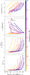 |
Fig. 6 Mass-loss rates, terminal wind velocities, wind efficiencies, and wind optical depths predicted from hydrodynamically consistent PoWRHD models as a function of stellar mass M*. The plots are colour-coded according to the different input inner boundary temperatures, ranging from T* = 50 to 12kK. |
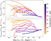 |
Fig. 7 Contribution of Fe-line acceleration at the critical point as a function of mass for different temperature sequences. Top : absolute contribution of Fe. Bottom : relative contribution of Fe to the total line acceleration. The contributions are normalised to gravity and expressed as Eddington parameters. The figure is colour-coded based on the temperature T*. |
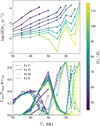 |
Fig. 8 Mass-loss rate as a function of stellar temperature, T*, for different masses. Top : predicted mass-loss rates. Bottom : relative contributions from relevant Fe wind-driving ions to the total line acceleration at the critical point. The radiative acceleration contributions are normalised to gravity and expressed as Eddington parameters. The curves are colour-coded by stellar mass. |
4.4 Mass-loss scaling with mass and temperature
In this section, we present a fitting relation to predict the massloss rate as a function of M* and T*. Since our investigation varies only these parameters, the following formula does not represent a complete mass-loss prescription. Rather, it is designed to capture the scaling relations and functional form, which will serve as a foundation for future work, as we plan to extend this relation by incorporating other relevant parameters in our grid such as luminosity and surface abundances.
Our fit combines a double-exponential mass scaling - capturing both shallow and steep scalings - with quadratic temperature dependence and Gaussian dips reproducing the bistability jumps. These Gaussian terms capture the mass-loss rate minima near T* ≈ 25kK and l5kK3:
![Mathematical equation: \begin{split} \log \dot{M}(M_\star,T_\star) &= a + \log \Big[ 10^{\,f_\mathrm{low}(M_\star)} + 10^{\,f_\mathrm{high}(M_\star)} \Big] \\[1pt] &\quad + b(M_\star)\,\log \!\left(T_\star/T_\mathrm{ref}\right) + c\,\big[\log \!\left(T_\star/T_\mathrm{ref}\right)\big]^2 \\[1pt] &\quad - G_1(M_\star) \, \exp\!\Bigg[ - \left(\dfrac{T_\star - T_1}{\sigma_T}\right)^2 \Bigg] \\ &\quad - G_2(M_\star) \, \exp\!\Bigg[ -\left(\dfrac{T_\star - T_2(M_\star)}{\sigma_T}\right)^2 \Bigg], \label{eq: mdot_fit} \end{split}](/articles/aa/full_html/2026/02/aa57298-25/aa57298-25-eq11.png) (10)
(10)
where M* is in solar masses and T* is in kK. The bistability temperatures T1 and T2(M*) mark the centres of the Gaussian dips, while σT controls their width. We fix T1 = 25 kK and σT = 2 kK during fitting, as our models demonstrate negligible variation of these parameters with mass or temperature. Stellar mass and temperature are normalised to references values, Mref and Tref, with Mref = 60 M⊙ at Tref = 38 kK. These normalisation values are not arbitrary - as demonstrated in Sect. 4.1, they roughly correspond to the M* and T* values required by our hydrodynamic models to reproduce the Arches Cluster transition mass-loss rate. The mass-dependent coefficients take the following form:
![Mathematical equation: \begin{aligned} a &= -5.527\,(\pm0.022) \\ f_\mathrm{low}(M_\star) &= -1.864\,(\pm0.198) \cdot\log(M_\star/M_\mathrm{ref}), \\ f_\mathrm{high}(M_\star) &= -9.865\,(\pm0.273)\cdot\log(M_\star/M_\mathrm{ref}) \\ b(M_\star) &= -2.062\,(\pm0.521) + 5.671\,(\pm1.536) \cdot\log(M_\star/M_\mathrm{ref}) \\ c &= 3.974\,(\pm0.459) \\ G_1(M_\star) &= 0.178\,(\pm0.042) \;\exp\big[9.611\,(\pm1.293) \cdot\log(M_\star/M_\mathrm{ref})\big] \\ G_2(M_\star) &= 0.291\,(\pm0.051) \;\exp\big[8.658\,(\pm1.048) \cdot \log(M_\star/M_\mathrm{ref})\big] \\ T_2(M_\star) &= 16.941\,(\pm0.268) - 7.274\,(\pm1.506) \cdot\log(M_\star/M_\mathrm{ref}), \\ M_\mathrm{ref} &= 60 - 0.521(\pm0.133) \cdot(T_\star-T_\mathrm{ref}) \\ T_1 &= 25\,\mathrm{kK}, \quad \sigma_T = 2\,\mathrm{kK}, \quad T_\mathrm{ref} = 38\,\mathrm{kK}. \end{aligned}](/articles/aa/full_html/2026/02/aa57298-25/aa57298-25-eq12.png)
Several simplifications help elucidate the different scaling relations in Eq. (10). Our fitting function ensures that at high temperatures (T* ≳ 30 kK) - beyond the influence of bistability features - the Gaussian corrections vanish, leaving only the baseline mass and temperature scaling. The double-exponential term 10fhigh(M*) + 10flow(M*) captures a critical feature: the transition from shallow to steep power-law scaling of log Ṁ versus log M* at higher temperatures. For the simplified case of T* = 38kK, Eq. (10) reduces to
![Mathematical equation: \log \dot{M}(M_\star,38\,\mathrm{kK}) \approx a + \log \left[ 10^{\,f_\mathrm{low}(M_\star)} + 10^{\,f_\mathrm{high}(M_\star)} \right],](/articles/aa/full_html/2026/02/aa57298-25/aa57298-25-eq13.png) (11)
(11)
which simplifies further depending on which term dominates based on the stellar mass relative to 60 M⊙. For high-mass stars with M* > 60 M⊙ or low Γe, the first term dominates, while for lower-mass stars, M* < 60 M⊙, with a high Γe, the second term takes over:
 (12)
(12)
The double-exponential term therefore accurately captures the shallow-to-steep transition in the log Ṁ versus log M* scaling predicted by our models. Figure 9 shows our fit relations, where for T* ≳ 30 kK, the log Ṁ versus log M* scaling steepens below M* ≈ 60 M⊙.
To understand how the baseline mass-loss rate scales with temperature, we fix M* = 60 M⊙. Neglecting the minor variation of Mref with T* and the double-Gaussian bistability dips, the fit relation reduces to
![Mathematical equation: \begin{split} \log \dot{M}(60\,M_\odot,T_\star) &\approx a + \mathrm{log}2 - 2.062\cdot \mathrm{log}(T_\star/38) \\ &\quad+\, 3.974\cdot\big[\log \!\left(T_\star/38\right)\big]^2 . \label{eq: mdot_fit_M_fixed_60} \end{split}](/articles/aa/full_html/2026/02/aa57298-25/aa57298-25-eq15.png) (13)
(13)
In Fig. 10, we show our fitted relation as a function of T* from Eq. (10), compared to our model predictions. The baseline scaling of log Ṁ(T*) with log T* exhibits a steep negative dependence. For example, at T* = 38 kK, differentiating Eq. (13) gives an instantaneous slope of  . As T* decreases, this slope further steepens. We also compare our predictions with reference lines showing a
  scaling, which arise from the geometrical effect of increasing radii and decreasing surface gravity. We find that in certain parameter regimes, the mass-loss scaling with temperature is dominated by this purely geometrical effect, particularly at higher Γe and lower T*.
We acknowledge a practical limitation of Eq. (10): the temperature T* is defined at an arbitrary Rosseland continuum optical depth of τR,cont = 20, which may not be readily accessible in stellar structure and evolution models (see e.g. the recent discussion in Josiek et al. 2025). Most structure codes compute the surface temperature Teff at the photospheric surface where τR = 2/3, assuming a static, grey atmosphere. Furthermore, due to the arbitrary choice of τR,cont, defining the effective temperature at τR = 2/3 provides a more physically meaningful measure of stellar temperature.
We therefore provide a supplementary relation connecting mass-loss rate with both T* and Teff(τR = 2/3) for our atmosphere models, enabling temperature parameter mapping based on the predicted Ṁ. Figure 11 illustrates the relationship between T* and Teff(τR = 2/3). The difference between the two temperatures increases with increasing mass-loss rate (cf. Smith et al. 2004; Sander et al. 2023), as the wind becomes more optically thick. We adopt a linear relation between T* and Teff (τR = 2/3), with both slope and y-intercept scaling with mass-loss rate:
 (14)
(14)
where
 (15)
(15)
Here, Ṁ is in M⊙ yr−1, while temperatures are in kK. The coefficients a(Ṁ) and b(Ṁ) are constructed such that at very low mass loss, the difference saturates to ∆T = T* - Teff (τR = 2/3) ~ 1 kK in agreement with our model predictions in Fig. 11. While the typical error from our T* fits is of the order of 1 kK, especially for the highest mass-loss rate models, it successfully captures the overall trend of increasing difference between the temperatures towards higher mass-loss rate. Therefore, given M* and Teff(τR = 2/3), an iterative solution of Eqs. (10) and (14) simultaneously yields Ṁ and T*.
While we present fits capturing the temperature mapping between T* and Teff(τR = 2/3) for the current set of atmosphere models, we emphasise that these relations are preliminary and should not be over-interpreted. For example, the Teff(τR = 2/3) values calculated in evolution models assume a grey static atmosphere connected to the outer boundary. Consequently, the Teff(τR = 2/3) from evolution models could be inaccurate, due to effects such as inflation and turbulence associated with the hot iron bump (see e.g. Josiek et al. 2025, for potential issues with connecting structure and atmosphere models). Additionally, since we varied only M* in this work, further testing with variations in other stellar parameters is necessary to establish whether this correction is universally applicable.
Finally, we perform a sanity check of our fitting relations using the transition mass-loss rate obtained from applying Eq. (9) to the transition objects in the Arches Cluster. Section 4.1 demonstrated that the mass-loss kink occurs at M* ≈ 60 M⊙. With mass dependencies normalised to 60 M⊙ and Teff(τR = 2/3) = 33.4kK, solving Eqs. (10) and (14) gives log Ṁ ≈ −5.22 (and T* = 38.05 kK). This value closely matches the Arches transition mass-loss rate, validating our fitting relations.
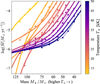 |
Fig. 9 PoWRHD predicted mass-loss rates (symbols with dashed lines) compared to our best-fit relation (solid lines) as functions of stellar mass, M*. The fit derives from Eq. (10), with lines colour-coded by stellar temperature, T*. |
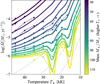 |
Fig. 10 Same as Fig. 9, but presenting mass-loss rates as functions of stellar temperature, T*, colour-coded by stellar mass, M*. The dashed black lines indicate reference scalings of |

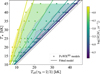 |
Fig. 11 Change in the inner boundary temperature T* as a function of the effective temperature defined at Rosseland optical depth τR = 2/3 as winds become optically thick. Symbols show our PoWRHD model predictions, colour-coded by mass-loss rate. Contours of constant massloss rate are shown with dashed lines, while solid lines denote the fits from Eq. (14). The dotted black line marks where the two temperatures are equal. |
5 Discussion: Comparison to previous works
We now place our model predictions in context with previous VMS wind investigations. Gräfener & Hamann (2008) examined VMS winds across a comparable parameter space using a precursor to our PoWRHD version. Our models improve upon theirs through expanded atomic data and broader coverage of the Γe - T* parameter space (see Appendix B). While Gräfener & Hamann (2008) identified steep scaling of mass loss with Γe, their predicted mass-loss rates lacked kink behaviour - possibly because their models did not cover the Γe < 0.4 regime where slope shallowing occurs in our calculations. We further check the absolute mass-loss rate predictions for M* = 60 M⊙ and T* = 38 kK where we identified our kink to match the transition mass-loss rate. There is roughly 0.2 dex difference between our predictions, with our rates higher compared to Gräfener & Hamann (2008) (see Fig. A.1). This difference could be due to our expanded atomic data, as well as our inclusion of turbulent pressure in the atmosphere.
For high-Γe VMSs, our models predict a steep mass-loss scaling with mass and consequently Γe of Ṁ ~ Γe10 (see Fig. 9). Although further work must establish whether such scaling persists in the Ṁ - Γe relation when varying luminosity and H content simultaneously, this exceeds the −5 scaling reported by Gräfener & Hamann (2008) and Vink et al. (2011).
The overlapping temperature range (30-50 kK) between our work and Gräfener & Hamann (2008) also reveals qualitative agreement between both studies: the baseline mass-loss rate increases with decreasing T*.
VMS winds were further studied using MC techniques by Vink et al. (2011), who predicted the kink behaviour. While qualitative agreement exists between our predictions, the location of the kink in our models occurs at Γe close to 0.4, lower compared to Vink et al. (2011). However, this is consistent with Vink et al. (2011) expectations that their kink would shift toward lower values.
6 Conclusions
In this paper, we have investigated VMS wind properties using hydrodynamically consistent PoWRHD stellar atmosphere models. We examined how stellar mass and temperature govern predicted mass-loss rates, terminal velocities, and wind characteristics across the parameter space relevant to WNh stars. Our principal findings are s follows:
Our models predict a characteristic upturn in the log Ṁ-log M relation for sequences with T* ≳ 30 kK, producing a kink feature consistent with Monte Carlo simulations of Vink et al. (2011) and empirical evidence from Bestenlehner et al. (2014). The location of the kink in the MC models roughly coincides with the crossing of the singlescattering limit and the wind optical depth reaching order unity. With multiple scattering in the wind, the star can drive a stronger mass-loss rate, resulting in the appearance of a kink. Our CMF-based models corroborate the MC results; for instance, our models also predict the characteristic kink feature where the wind optical depth crosses unity, and the synthetic spectra transition from absorption-dominated O-type to emission-dominated H-rich WR morphologies. The wind efficiency parameter reaches η ~ 0.45 at the kink - slightly below the η - 0.6 predicted by Vink & Gräfener (2012). This discrepancy likely reflects our underprediction of terminal velocities compared to those inferred for transition-type stars in the Arches Cluster. For the chosen luminosity, the kink occurs at M* ≈ 60 M⊙ corresponding to Γe ≈ 0.43;
We tested our predictions against the model-independent transition mass-loss rate in the Arches Cluster near the Galactic center, offering a crucial first-order sanity check for any prescribed mass loss at the O to WNh boundary. Our mass-loss rates match the Arches transition value of log(Ṁtrans) ≈ −5.16 (Vink & Gräfener 2012) at our predicted kink location. Importantly, we also reproduce the associated spectroscopic transition from absorption- to emission-dominated Hβ profiles as the wind optical depth passes unity, thereby confirming the physical interpretation of the transition mass-loss concept and its connection to optically thick wind onset in VMSs;
In addition to the kink, our models reveal dramatic temperature-dependent jumps in the predicted mass-loss rates, most prominently at T* ≈ 25 and 15kK. These features arise from shifts in the dominant Fe ionisation stage - FeIV → FeIII near 25kK and FeIII → FeII near 15kK -creating radiative driving deficits where both upper and lower ionisation stages dominate. The resulting bistability jumps agree qualitatively with Monte Carlo line-driven wind predictions from both globally and locally consistent models (Vink et al. 1999; Vink 2018; Vink & Sander 2021), as well as CMFGEN and METUJE computations (Petrov et al. 2016; Krticka et al. 2021). At these specific temperatures, our predicted log Ṁ-log M relation maintains steep scaling throughout the investigated mass range;
A radiative acceleration analysis reveals the decisive role of Fe-group elements, which - despite low abundances -contribute over 50% of total line driving through myriad UV transitions. In the sub-critical wind regime where Ṁ is set, continuum processes alone are insufficient to overcome gravity and Fe line transitions initiate the wind;
-
To facilitate further applications, we provide fitting prescriptions (Equations (10) and (14)) that reproduce both the kink and the bistability behaviour. These relations combine a double-exponential mass scaling with Gaussian terms capturing the ionisation-driven minima, thereby encoding the complex temperature and mass dependencies. Although derived for fixed luminosity and composition, these formulae establish a quantitative foundation for future incorporation of additional parameters including luminosity, surface H fraction, and metallicity.
Together, these results represent significant progress toward predictive VMS mass-loss prescriptions. By capturing both the Eddington-parameter associated kink behaviour and Feionisation shift driven bistable winds, our hydrodynamically consistent models address fundamental gaps in VMS wind theory, with implications for stellar evolution, chemical feedback, and stellar fate.
Acknowledgements
We thank the anonymous referee for constructive comments that helped improve the paper. GNS and JSV are supported by STFC funding under grant number ST/Y001338/1. AACS is supported by the German Deutsche Forschungsgemeinschaft, DFG in the form of an Emmy Noether Research Group - Project-ID 445674056 (SA4064/1-1, PI: Sander). AACS further acknowledges financial support by the Federal Ministry for Economic Affairs and Climate Action (BMWK) via the German Aerospace Center (Deutsches Zentrum für Luft- und Raumfahrt, DLR) grant 50 OR 2503 (PI: Sander). This project was co-funded by the European Union (Project 101183150 - OCEANS).
References
- Bernini-Peron, M., Sander, A. A. C., Najarro, F., et al. 2025, A&A, 697, A41 [NASA ADS] [CrossRef] [EDP Sciences] [Google Scholar]
- Bestenlehner, J. M., Vink, J. S., Gräfener, G., et al. 2011, A&A, 530, L14 [NASA ADS] [CrossRef] [EDP Sciences] [Google Scholar]
- Bestenlehner, J. M., Gräfener, G., Vink, J. S., et al. 2014, A&A, 570, A38 [NASA ADS] [CrossRef] [EDP Sciences] [Google Scholar]
- Brands, S. A., de Koter, A., Bestenlehner, J. M., et al. 2022, A&A, 663, A36 [Google Scholar]
- Cameron, A. J., Saxena, A., Bunker, A. J., et al. 2023, A&A, 677, A115 [NASA ADS] [CrossRef] [EDP Sciences] [Google Scholar]
- Castor, J. I., Abbott, D. C., & Klein, R. I. 1975, ApJ, 195, 157 [Google Scholar]
- Charbonnel, C., Schaerer, D., Prantzos, N., et al. 2023, A&A, 673, L7 [NASA ADS] [CrossRef] [EDP Sciences] [Google Scholar]
- Crowther, P. A., & Walborn, N. R. 2011, MNRAS, 416, 1311 [Google Scholar]
- Crowther, P. A., Lennon, D. J., & Walborn, N. R. 2006, A&A, 446, 279 [NASA ADS] [CrossRef] [EDP Sciences] [Google Scholar]
- Crowther, P. A., Schnurr, O., Hirschi, R., et al. 2010, MNRAS, 408, 731 [Google Scholar]
- Crowther, P. A., Caballero-Nieves, S. M., Bostroem, K. A., et al. 2016, MNRAS, 458, 624 [Google Scholar]
- Curti, M., Witstok, J., Jakobsen, P., et al. 2025, A&A, 697, A89 [Google Scholar]
- de Koter, A., Heap, S. R., & Hubeny, I. 1998, ApJ, 509, 879 [Google Scholar]
- Debnath, D., Sundqvist, J. O., Moens, N., et al. 2024, A&A, 684, A177 [NASA ADS] [CrossRef] [EDP Sciences] [Google Scholar]
- Figer, D. F. 2005, Nature, 434, 192 [Google Scholar]
- Friend, D. B., & Abbott, D. C. 1986, ApJ, 311, 701 [Google Scholar]
- Gieles, M., Padoan, P., Charbonnel, C., Vink, J. S., & Ramírez-Galeano, L. 2025, MNRAS, 544, 483 [Google Scholar]
- Gräfener, G., & Hamann, W. R. 2005, A&A, 432, 633 [NASA ADS] [CrossRef] [EDP Sciences] [Google Scholar]
- Gräfener, G., & Hamann, W. R. 2008, A&A, 482, 945 [Google Scholar]
- Gräfener, G., Koesterke, L., & Hamann, W. R. 2002, A&A, 387, 244 [NASA ADS] [CrossRef] [EDP Sciences] [Google Scholar]
- Gräfener, G., Owocki, S. P., Grassitelli, L., & Langer, N. 2017, A&A, 608, A34 [NASA ADS] [CrossRef] [EDP Sciences] [Google Scholar]
- Grevesse, N., & Sauval, A. J. 1998, Space Sci. Rev., 85, 161 [Google Scholar]
- Groh, J. H., Hillier, D. J., Damineli, A., et al. 2009, ApJ, 698, 1698 [NASA ADS] [CrossRef] [Google Scholar]
- Hamann, W. R. 1985, A&A, 148, 364 [Google Scholar]
- Hamann, W. R. 1986, A&A, 160, 347 [NASA ADS] [Google Scholar]
- Hamann, W. R., & Gräfener, G. 2003, A&A, 410, 993 [CrossRef] [EDP Sciences] [Google Scholar]
- Hamann, W. R., & Koesterke, L. 1998, A&A, 335, 1003 [Google Scholar]
- Higgins, E. R., Vink, J. S., Sabhahit, G. N., & Sander, A. A. C. 2022, MNRAS, 516, 4052 [NASA ADS] [CrossRef] [Google Scholar]
- Higgins, E. R., Vink, J. S., Hirschi, R., Laird, A. M., & Sabhahit, G. N. 2023, MNRAS, 526, 534 [NASA ADS] [CrossRef] [Google Scholar]
- Higgins, E. R., Vink, J. S., Hirschi, R., Laird, A. M., & Sabhahit, G. 2025, A&A, 699, A71 [NASA ADS] [CrossRef] [EDP Sciences] [Google Scholar]
- Hillier, D. J., Lanz, T., Heap, S. R., et al. 2003, ApJ, 588, 1039 [Google Scholar]
- Hirschi, R. 2015, in Astrophysics and Space Science Library, 412, Very Massive Stars in the Local Universe, ed. J. S. Vink, 157 [Google Scholar]
- Isobe, Y., Ouchi, M., Tominaga, N., et al. 2023, ApJ, 959, 100 [NASA ADS] [CrossRef] [Google Scholar]
- Ji, X., Belokurov, V., Maiolino, R., et al. 2025, MNRAS [arXiv:2505.12505] [Google Scholar]
- Josiek, J., Sander, A. A. C., Bernini-Peron, M., et al. 2025, A&A, 697, A193 [NASA ADS] [CrossRef] [EDP Sciences] [Google Scholar]
- Kalari, V. M., Horch, E. P., Salinas, R., et al. 2022, ApJ, 935, 162 [NASA ADS] [CrossRef] [Google Scholar]
- Köhler, K., Langer, N., de Koter, A., et al. 2015, A&A, 573, A71 [NASA ADS] [CrossRef] [EDP Sciences] [Google Scholar]
- Krticka, J., Kubát, J., & Krticková, I. 2021, A&A, 647, A28 [NASA ADS] [CrossRef] [EDP Sciences] [Google Scholar]
- Krumholz, M. R. 2015, in Astrophysics and Space Science Library, 412, Very Massive Stars in the Local Universe, ed. J. S. Vink, 43 [Google Scholar]
- Lamers, H. J. G. L. M., & Cassinelli, J. P. 1999, Introduction to Stellar Winds [Google Scholar]
- Lefever, R. R., Sander, A. A. C., Bernini-Peron, M., et al. 2025, A&A, 700, A2 [NASA ADS] [CrossRef] [EDP Sciences] [Google Scholar]
- Lucy, L. B., & Abbott, D. C. 1993, ApJ, 405, 738 [Google Scholar]
- Lucy, L. B., & Solomon, P. M. 1970, ApJ, 159, 879 [Google Scholar]
- Martins, F. 2015, in Astrophysics and Space Science Library, 412, Very Massive Stars in the Local Universe, ed. J. S. Vink, 9 [Google Scholar]
- Martins, F., Hillier, D. J., Paumard, T., et al. 2008, A&A, 478, 219 [NASA ADS] [CrossRef] [EDP Sciences] [Google Scholar]
- Massey, P., & Hunter, D. A. 1998, ApJ, 493, 180 [NASA ADS] [CrossRef] [Google Scholar]
- Mihalas, D., Kunasz, P. B., & Hummer, D. G. 1975, ApJ, 202, 465 [CrossRef] [Google Scholar]
- Muijres, L. E., de Koter, A., Vink, J. S., et al. 2011, A&A, 526, A32 [NASA ADS] [CrossRef] [EDP Sciences] [Google Scholar]
- Müller, P. E., & Vink, J. S. 2008, A&A, 492, 493 [NASA ADS] [CrossRef] [EDP Sciences] [Google Scholar]
- Oey, M. S., & Clarke, C. J. 2005, ApJ, 620, L43 [NASA ADS] [CrossRef] [Google Scholar]
- Pauldrach, A., Puls, J., & Kudritzki, R. P. 1986, A&A, 164, 86 [NASA ADS] [Google Scholar]
- Petrov, B., Vink, J. S., & Gräfener, G. 2016, MNRAS, 458, 1999 [NASA ADS] [CrossRef] [Google Scholar]
- Sabhahit, G. N., Vink, J. S., Higgins, E. R., & Sander, A. A. C. 2022, MNRAS, 514, 3736 [NASA ADS] [CrossRef] [Google Scholar]
- Sabhahit, G. N., Vink, J. S., Sander, A. A. C., & Higgins, E. R. 2023, MNRAS, 524, 1529 [NASA ADS] [CrossRef] [Google Scholar]
- Sabhahit, G. N., Vink, J. S., Sander, A. A. C., et al. 2025, A&A, 696, A200 [NASA ADS] [CrossRef] [EDP Sciences] [Google Scholar]
- Sander, A., Shenar, T., Hainich, R., et al. 2015, A&A, 577, A13 [NASA ADS] [CrossRef] [EDP Sciences] [Google Scholar]
- Sander, A. A. C. 2015, PhD thesis, University of Potsdam, Germany [Google Scholar]
- Sander, A. A. C., & Vink, J. S. 2020, MNRAS, 499, 873 [Google Scholar]
- Sander, A. A. C., Hamann, W. R., Todt, H., Hainich, R., & Shenar, T. 2017, A&A, 603, A86 [NASA ADS] [CrossRef] [EDP Sciences] [Google Scholar]
- Sander, A. A. C., Vink, J. S., & Hamann, W. R. 2020, MNRAS, 491, 4406 [Google Scholar]
- Sander, A. A. C., Lefever, R. R., Poniatowski, L. G., et al. 2023, A&A, 670, A83 [NASA ADS] [CrossRef] [EDP Sciences] [Google Scholar]
- Senchyna, P., Plat, A., Stark, D. P., et al. 2024, ApJ, 966, 92 [NASA ADS] [CrossRef] [Google Scholar]
- Smith, N., Vink, J. S., & de Koter, A. 2004, ApJ, 615, 475 [NASA ADS] [CrossRef] [Google Scholar]
- Topping, M. W., Stark, D. P., Senchyna, P., et al. 2024, MNRAS, 529, 3301 [NASA ADS] [CrossRef] [Google Scholar]
- Upadhyaya, A., Marques-Chaves, R., Schaerer, D., et al. 2024, A&A, 686, A185 [NASA ADS] [CrossRef] [EDP Sciences] [Google Scholar]
- Vink, J. S. 2018, A&A, 615, A119 [NASA ADS] [CrossRef] [EDP Sciences] [Google Scholar]
- Vink, J. S. 2022, ARA&A, 60, 203 [Google Scholar]
- Vink, J. S. 2023, A&A, 679, L9 [NASA ADS] [CrossRef] [EDP Sciences] [Google Scholar]
- Vink, J. S., & Gräfener, G. 2012, ApJ, 751, L34 [Google Scholar]
- Vink, J. S., & Sander, A. A. C. 2021, MNRAS, 504, 2051 [NASA ADS] [CrossRef] [Google Scholar]
- Vink, J. S., de Koter, A., & Lamers, H. J. G. L. M. 1999, A&A, 350, 181 [Google Scholar]
- Vink, J. S., de Koter, A., & Lamers, H. J. G. L. M. 2000, A&A, 362, 295 [Google Scholar]
- Vink, J. S., de Koter, A., & Lamers, H. J. G. L. M. 2001, A&A, 369, 574 [NASA ADS] [CrossRef] [EDP Sciences] [Google Scholar]
- Vink, J. S., Muijres, L. E., Anthonisse, B., et al. 2011, A&A, 531, A132 [NASA ADS] [CrossRef] [EDP Sciences] [Google Scholar]
- Weidner, C., & Kroupa, P. 2004, MNRAS, 348, 187 [NASA ADS] [CrossRef] [Google Scholar]
- Wofford, A., Leitherer, C., Chandar, R., & Bouret, J.-C. 2014, ApJ, 781, 122 [Google Scholar]
Table B.3 in Appendix B provides a tabulation of the explored parameter space along with relevant wind predictions.
This is because the radiative acceleration arad is re-calculated every iteration as a function of radius. This is unlike CAK-type approaches where the arad is parametrised as a function of radius and velocity gradient, and the resulting CAK-critical point does not coincide with the sonic point.
All logarithms in the fitting formula are base 10.
Appendix A Additional plots
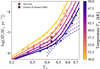 |
Fig. A.1 Mass-loss rate versus the classical Eddington parameter Γe, comparing our predictions with those of Gräfener & Hamann (2008). Our model predictions are indicated by coloured symbols connected with dashed lines. The best-fit relation from Eq (10) is shown as solid lines, while the fit from Gräfener & Hamann (2008) is shown as dotted lines. Absolute mass-loss rates predicted by the two fits for M* = 60 M⊙ and T* = 38 kK are indicated by red and black star symbols, respectively. |
Appendix B Parameter space and predicted wind properties
In our PoWRHD models, we use an extended set of 17 elements with their respective mass fractions provided in Table B.1. The total metal mass fraction adds up to Z = 0.02 with individual metal mass fractions distributed following solar-scaled abundances from Grevesse & Sauval (1998). The detailed breakdown of the relevant ion list and their respective level and line numbers are provided in Table B.2.
Mass fractions of elements used in the ‘base model’ (Z = 0.02).
List of ions and their corresponding level and line numbers used in our PoWRHD models.
Predicted wind properties from PoWRHD models for input stellar mass and temperature.
All Tables
List of ions and their corresponding level and line numbers used in our PoWRHD models.
Predicted wind properties from PoWRHD models for input stellar mass and temperature.
All Figures
|
Fig. 1 Total radiative acceleration and its contributions from continuum processes and line transitions. Decomposition of the total radiative acceleration (solid black) into continuum (dashed green) and line (dashed red) components along with individual contributions from constituent elements in the atmosphere (coloured lines with symbols, see legend). Each of these element contributions consists of the sum of their line and continuum accelerations. All accelerations are normalised to gravity. The dotted and dashed vertical grey lines mark the sonic and critical points, Rsonic and Rcrit, respectively. The model stellar parameters are log(L*/L⊙) = 6.0, M* = 105 M⊙, T* = 35kK, X = 0.7, and Z = 0.02. |
| In the text | |
|
Fig. 2 Contributions from electron scattering, free-free and bound-free continuum transitions, and line transitions of individual elements at the critical point, shown as a function of mass. The contributions are normalised to gravity and expressed as Eddington parameters. Top : absolute contributions from different opacity sources. Bottom : relative line contributions from different elements. The model sequence corresponds to a temperature of T* = 35 kK. |
| In the text | |
|
Fig. 3 Testing the PoWRHD model predictions against the transition mass-loss rate in the Arches Cluster. Left : predicted mass-loss rates versus stellar mass from PoWRHD models for the T* = 35 kK sequence (solid black) and from Vink et al. (2000) (dotted blue), compared to the transition mass-loss rate of log(M) ≈ −5.16 in the Arches (horizontal red line) from Vink & Gräfener (2012). The PoWRHD models are computed with fixed log(L*/L⊙) = 6.0, X = 0.7, and Z = 0.02, roughly matching the observed properties of the Arches transition objects (Martins et al. 2008). The T* = 35 kK sequence shown has surface temperatures close to the observed Teff(τR = 2/3) ≈ 33.4 kK of the transition objects. The stellar masses of the transition objects span ~55—75 M⊙ corresponding to their averaged luminosity and temperature. Middle : predicted wind efficiency parameter versus mass compared to the transition value η ≈ 0.6 (dashed red) from Vink & Gräfener (2012). Right : predicted wind optical depth versus mass compared to the transition value τF(rsonic) ≈ 1 (dashed red) from Vink & Gräfener (2012). |
| In the text | |
|
Fig. 4 Synthetic spectra showing relevant wind lines in the optical for the T* = 35 kK model sequence presented in Fig. 3. The spectra are colour-coded based on the stellar mass. |
| In the text | |
|
Fig. 5 Synthetic spectra showing relevant wind lines in the UV for the T* = 35 kK model sequence presented in Fig. 3. The spectra are colour-coded based on the stellar mass. |
| In the text | |
|
Fig. 6 Mass-loss rates, terminal wind velocities, wind efficiencies, and wind optical depths predicted from hydrodynamically consistent PoWRHD models as a function of stellar mass M*. The plots are colour-coded according to the different input inner boundary temperatures, ranging from T* = 50 to 12kK. |
| In the text | |
|
Fig. 7 Contribution of Fe-line acceleration at the critical point as a function of mass for different temperature sequences. Top : absolute contribution of Fe. Bottom : relative contribution of Fe to the total line acceleration. The contributions are normalised to gravity and expressed as Eddington parameters. The figure is colour-coded based on the temperature T*. |
| In the text | |
|
Fig. 8 Mass-loss rate as a function of stellar temperature, T*, for different masses. Top : predicted mass-loss rates. Bottom : relative contributions from relevant Fe wind-driving ions to the total line acceleration at the critical point. The radiative acceleration contributions are normalised to gravity and expressed as Eddington parameters. The curves are colour-coded by stellar mass. |
| In the text | |
|
Fig. 9 PoWRHD predicted mass-loss rates (symbols with dashed lines) compared to our best-fit relation (solid lines) as functions of stellar mass, M*. The fit derives from Eq. (10), with lines colour-coded by stellar temperature, T*. |
| In the text | |
|
Fig. 10 Same as Fig. 9, but presenting mass-loss rates as functions of stellar temperature, T*, colour-coded by stellar mass, M*. The dashed black lines indicate reference scalings of |
| In the text | |
|
Fig. 11 Change in the inner boundary temperature T* as a function of the effective temperature defined at Rosseland optical depth τR = 2/3 as winds become optically thick. Symbols show our PoWRHD model predictions, colour-coded by mass-loss rate. Contours of constant massloss rate are shown with dashed lines, while solid lines denote the fits from Eq. (14). The dotted black line marks where the two temperatures are equal. |
| In the text | |
|
Fig. A.1 Mass-loss rate versus the classical Eddington parameter Γe, comparing our predictions with those of Gräfener & Hamann (2008). Our model predictions are indicated by coloured symbols connected with dashed lines. The best-fit relation from Eq (10) is shown as solid lines, while the fit from Gräfener & Hamann (2008) is shown as dotted lines. Absolute mass-loss rates predicted by the two fits for M* = 60 M⊙ and T* = 38 kK are indicated by red and black star symbols, respectively. |
| In the text | |
Current usage metrics show cumulative count of Article Views (full-text article views including HTML views, PDF and ePub downloads, according to the available data) and Abstracts Views on Vision4Press platform.
Data correspond to usage on the plateform after 2015. The current usage metrics is available 48-96 hours after online publication and is updated daily on week days.
Initial download of the metrics may take a while.