| Issue |
A&A
Volume 706, February 2026
|
|
|---|---|---|
| Article Number | A23 | |
| Number of page(s) | 17 | |
| Section | Cosmology (including clusters of galaxies) | |
| DOI | https://doi.org/10.1051/0004-6361/202557496 | |
| Published online | 27 January 2026 | |
The eventful life journey of galaxy clusters
II. Impact of mass accretion on the thermodynamic structure of the ICM
1
Dipartimento di Fisica e Astronomia, Università di Bologna Via Piero Gobetti 93/2 IT-40129 Bologna, Italy
2
Departament d’Astronomia i Astrofísica, Universitat de València ES-46100 Burjassot València, Spain
3
Observatori Astronòmic, Universitat de València ES-46980 Paterna València, Spain
★ Corresponding author: This email address is being protected from spambots. You need JavaScript enabled to view it.
Received:
30
September
2025
Accepted:
9
December
2025
Abstract
Context. The internal structure of the intracluster medium (ICM) is tightly linked to the assembly history and physical processes in groups and clusters, but the role of recent accretion in shaping these profiles has not been fully explored.
Aims. We investigate the extent to which mass accretion accounts for variations in ICM density and thermodynamic profiles, and what present-day structures reveal about their formation histories.
Methods. We analyse a hydrodynamical cosmological simulation including gas cooling without feedback, to isolate the effects of heating from structure formation. Median profiles of ICM quantities are introduced as a robust description of the bulk ICM. We then examine correlations between mass accretion rates or assembly indicators with temperature, entropy, pressure, gas, and dark-matter density profiles, in addition to their scatter.
Results. Accretion in the last dynamical time strongly lowers central gas densities, while leaving dark matter largely unaffected, producing a distinct signature in the baryon depletion function. Pressure and entropy show the clearest dependence on accretion, whereas temperature is less sensitive. The radii of steepest entropy, temperature, and pressure shift inwards by ∼(10 − 20)% between high- and low-accretion subsamples. Assembly-state indicators are also related to the location of these features, and accretion correlates with the parameters of common fitting functions for density, pressure, and entropy.
Conclusions. Recent accretion leaves measurable imprints on the ICM structure, highlighting the potential of thermodynamic profiles as diagnostics of cluster growth history.
Key words: methods: numerical / methods: statistical / galaxies: clusters: general / galaxies: clusters: intracluster medium / galaxies: groups: general / large-scale structure of Universe
© The Authors 2026
 Open Access article, published by EDP Sciences, under the terms of the Creative Commons Attribution License (https://creativecommons.org/licenses/by/4.0), which permits unrestricted use, distribution, and reproduction in any medium, provided the original work is properly cited.
This article is published in open access under the Subscribe to Open model. This email address is being protected from spambots. You need JavaScript enabled to view it. to support open access publication.
1. Introduction
Most of the baryons in galaxy clusters reside in a hot, diffuse phase known as the intracluster medium (ICM), with typical number densities ranging n ∼ 10[ − 5, − 1] cm−3. Together with the even more diffuse warm-hot intergalactic medium (WHIM), they extend out to several virial radii (Davé et al. 2001; Walker et al. 2019). As their dominant baryonic component, the ICM1 is central to our understanding of galaxy clusters, the largest virialised systems in the Universe, as it provides a record of the gravitational and non-gravitational processes at play during cluster assembly (e.g. Kravtsov & Borgani 2012; Planelles et al. 2015).
As the diffuse gas from the intergalactic medium falls into the dark matter (DM) halo potential well, the ICM emerges as an almost fully ionised plasma and reaches temperatures of ∼10[7, 8] K due to adiabatic and shock compression (Evrard 1990; Quilis et al. 1998). The dissipation of turbulent motions, naturally arising during hierarchical assembly (Dolag et al. 2005; Vazza et al. 2017), together with a plethora of non-gravitational processes (e.g. feedback from star formation and active galactic nuclei, McNamara & Nulsen 2007, as well as microphysical transport processes, Walker et al. 2019), all alter the properties and distribution of diffuse baryons. Altogether, these mechanisms determine the radial structure of fundamental ICM quantities, such as density, temperature, entropy, and pressure.
The thermal ICM can be observed directly in the X-ray band, where its continuum (bremsstrahlung) and line emission inform on gas density, temperature, and metallicity (Böhringer & Werner 2010). Complementary information can be obtained in the microwave band from the Sunyaev & Zeldovich (1972, SZ) effect, which probes the integrated pressure of the hot electrons (Mroczkowski et al. 2019). Large campaigns in both bands (either separately, Merloni et al. 2024; ACTDESHSC Collaboration 2025, or in combination, Eckert et al. 2019) have provided constraints on the average profiles and their intrinsic scatter. Near-to-mid future instruments (NEWATHENA, Cruise et al. 2025; SIMONS OBSERVATORY, Abitbol et al. 2025) will likely extend the radial range towards cluster outskirts and increase the sample sizes, reaching higher redshifts.
In this context, accurate theoretical modelling is crucial to deriving the most from current and future observational efforts. At its most basic, clusters have been analytically described within the self-similar model (Kaiser 1986) using simple rescaling prescriptions. However, departures from self-similarity have been both predicted from simulations (Borgani et al. 2004) and observed (Arnaud et al. 2005) for decades. Clusters are dynamically young objects with very diverse assembly histories (Wong & Taylor 2012; Vallés-Pérez et al. 2020, 2025a, herein Paper I), environments (Kuchner et al. 2020), and internal processes (e.g. Le Brun et al. 2014), which imprint substantial variability in their internal structure and thermodynamic state.
Within this picture, simulations – which allow us to track the whole evolution of these systems – become essential tools to link the assembly history of clusters to their internal structure. In particular, several studies have sought to constrain the baryon distribution under different feedback models and across a range of radial apertures (Planelles et al. 2013; Battaglia et al. 2013; Angelinelli et al. 2022; Rasia et al. 2025), while also looking at how accretion and mergers shape the gas fractions (and, in turn, X-ray detectability, Marini et al. 2025). Regarding ICM thermodynamics, Hernández-Martínez et al. (2025) recently studied the thermodynamic profiles of local cluster analogues in relation to their assembly histories and cool-coredness (also closely related to dynamical state). Bridging the gap with observations, Biffi et al. (2013) investigated the relation between the kinematic state of the ICM (as a proxy for dynamical state) and X-ray luminosity, while De Luca et al. (2021) examined the complex relation of X-ray and SZ morphology (including, for instance, radial scatter and concentration), and 3D measures of cluster assembly.
Perhaps the study most directly addressing the connection between ICM thermodynamics and cluster assembly is Lau et al. (2015), who looked at the impact of mass accretion (quantified from the radial velocity near the virial radius, Rvir) in a non-radiative simulation on the pressure, temperature, and entropy profiles, with a special focus on cluster outskirts. The main trend reported by the authors corresponds to a shift in the location of the accretion shock, with stronger accretion pushing this feature inwards. In contrast, the impact on central regions is reduced. This likely stems from the absence of cooling mechanisms, which render heating from structure formation processes less important. A more recent analysis based on the FLAMINGO simulations has also explored how the density and temperature profiles of the hot gas vary with halo accretion rates, although with a broader focus on feedback effects (Magnus et al. 2025).
Building upon previous literature, we aim in this work to establish the effect of cluster mass growth – from either mergers or smooth accretion – on the ICM profiles across their whole radial extent. To do so, we analyse a cosmological hydrodynamical simulation that account for gas cooling, but without feedback mechanisms, allowing us to isolate the heating due to structure formation processes. In particular, we aim to assess: (i) the impact of selecting clusters by their recent accretion rates on their internal structures, (ii) the extent to which accretion explains the deviations from self-similarity in the profiles, (iii) whether commonly used assembly state indicators constrain the thermodynamic profiles; and (iv) beyond their central tendency, what can be said about the intrinsic scatter of the profiles.
The manuscript is organised as follows. In Sect. 2 we introduce the simulation set-up and the main analysis techniques. The results are presented in several subsections within Sect. 3. Finally, we further discuss our results and place them in the context of the literature in Sect. 4. Appendices A–D contain several additional tests and details.
2. Methods
Here, we present the key methodological aspects of this study, beginning in Sect. 2.1 with our simulation and cluster catalogue. The method for extracting radial profiles and stacking them are then covered, respectively, in Sects. 2.2 and 2.3.
2.1. The simulation and cluster catalogue
The present analyses are based on a Λ-cold dark matter (ΛCDM) N-Body plus hydrodynamical simulation, previously employed in earlier studies (e.g. Vallés-Pérez et al. 2024 and Paper I). For completeness, we provide here a succinct description of the simulation details, referring the reader to those references for further discussion.
The simulation tracks the evolution of a periodic cube of comoving side L = 100 h−1 Mpc, in a flat ΛCDM cosmology with matter density Ωm = 0.31, baryon fraction fb = 0.155, Hubble dimensionless parameter h = 0.678, and primordial power spectrum given by the index ns = 0.96 and the normalisation σ8 = 0.82, consistent with Planck Collaboration VI (2020) constraints. The initial conditions, set at zini = 100, were evolved in time with the adaptive mesh refinement (AMR) code MASCLET (Quilis 2004), accounting for gravitational and hydrodynamical forces as well as gas cooling. Neither star formation nor feedback was accounted for in this run. The deliberate choice of this set-up was motivated by the fact that, while it may produce unrealistic thermodynamic distributions in cluster cores due to excessive, unopposed cooling, it serves to isolate the effect of cluster assembly (gas accretion and mergers) on the thermodynamic state of the ICM, without confusion due to other (non-gravitational) heating feedback mechanisms. The coarsest and peak spatial resolutions are Δxbase = 576 kpc and Δxpeak = 9 kpc, where refinement is triggered by overdensities and converging flows. Base and peak DM mass resolutions are MDM, base = 7.7 × 10⁹ M⊙ and MDM, peak = 1.5 × 10⁷ M⊙. The effective refinement is such that ≳50% of the mass within Rvir of our cluster sample is resolved at Δx5 = 18 kpc resolution at z = 0 or better2.
Cluster catalogues were extracted from the DM distribution with the public halo finder ASOHF (Planelles & Quilis 2010; Knebe et al. 2011; Vallés-Pérez et al. 2022). For all purposes within this work, the density peak of the DM distribution was chosen to be the centre of the cluster. The basic sample, constructed at z = 0, consists of 31 clusters (above  ) and 358 groups (
 ). As we assume self-similarity to rescale the profiles (see Sect. 2.3 below), unless stated otherwise, we refer throughout this article to the whole sample as clusters to simplify notation, even though it includes clusters and groups.
Table 1 summarises in greater detail the mass composition of the selected systems, as well as their hot gas. The median gas fraction at R200m, over the whole sample, lies around (80−85)% of the cosmic value, consistent with the baryon fractions for ∼1014 M⊙ clusters reported by, for example, Angelinelli et al. (2022) using the MAGNETICUM suite. At lower masses (which dominate our sample), this baryon fraction in sensibly higher than the values reported in the literature, which range around (60−70)% of the cosmic value, as a consequence of over-cooling. While the present analysis is restricted to z = 0, merger trees obtained from tracking the most bound particles were used to compute the accretion rates Γ200m = dlog M200m/dlog a over the last dynamical time (τdyn), as discussed in Paper I.
Summary statistics accounting for the mass distribution of our group and cluster sample.
2.2. Profile making
Most customarily, radial profiles of additive (i.e. extensive; e.g. mass) quantities are obtained by summing over the resolution elements (either cells or particles) in pre-defined radial shells and normalising by the integration volume to define the corresponding density. For intensive quantities (e.g. temperature), the values are instead computed by averaging over the elements in the shell, possibly allowing for a weighting function (e.g. mass or emission).
This direct procedure has, however, a number of drawbacks. First, the finite width of the shells needs to be carefully tuned, since shells that are too wide can smear out the profile and be dominated by extreme values, especially when slopes are steep. Conversely, shells that are too narrow are noisy due to low-number statistics. Second, when considering mean profiles, the effect of clumps or very anisotropic environments (the latter, especially in cluster outskirts) dominates the value of the profiles. However, these contributions do not reflect the bulk ICM, since the dynamics of these structures (accounting for a significant fraction of cluster baryons, but a negligible volume; see e.g. Angelinelli et al. 2021) are usually decoupled from the smooth, volume-filling gas. While the first caveat is usually corrected by carefully tuning the binning (which in turn depends on resolution), the second needs ad hoc clump and substructure-removal steps, yielding profiles that depend continuously on the free parameters of these cleaning procedures (e.g. Zhuravleva et al. 2013).
In observations, it has become fairly common to employ the azimuthal median technique (Eckert et al. 2015 and subsequent studies, e.g. Ghirardini et al. 2019; also studied in the context of projected profiles from simulations, e.g. Ansarifard et al. 2020; Towler et al. 2023) to alleviate the emissivity bias due to strongly overdense clumps and recover the thermodynamic state of the smooth, volume-filling ICM3. This was partly motivated by Zhuravleva et al. (2013), who quantified the properties of clumps in simulated ICMs and argued that median profiles can better represent the bulk properties of the ICM. Nevertheless, in 3D profiles from simulations, the predominant practice is still to use mean profiles, most often with some substructure-excision procedure.
In contrast to the more common radial binning methods, in this work we adopted an alternative procedure to extract 3D profiles by computing, at each radius r, the median value of the quantities of interest (f) over Nθ × Nϕ angular directions, equally spaced in the unit sphere:
 (1)
(1)
To determine f(r, θ, ϕ), we evaluate the quantity of interest at the Cartesian coordinates corresponding to (r, θ, ϕ), by trilinear interpolation among the eight neighbouring cells at the highest available level of the AMR hierarchy, limited so that the local cell size does not fall below the radial spacing Δr. These profiles naturally account for the volume-filling, hot ICM, without the need for imposing any temperature threshold or explicit substructure removal step. Compared to the median profiles of Zhuravleva et al. (2013), this procedure has the additional advantage of being insensitive to any radial bin width. We illustrate the properties of these profiles and compare them to mean and mode profiles in Sect. 3.1.
2.3. Profile stacking
Stacked profiles (used in Sects. 3.2, 3.3, and 3.6) of a given quantity, X(r), over a given sample were computed by:
-
obtaining the individual profiles of the quantity of interest, X(r), from4rmin = 0.01R200m to rmax = 4R200m, with Δlog r = 0.01 dex;
-
rescaling the individual profiles to 𝒳(ℛ)≡X(ℛ ⋅ Rnorm)/Xnorm, where ℛ is the radius in units of Rnorm = R200m and the normalisation constants Xnorm correspond to the self-similar values specified in Appendix A;
-
resampling the profiles to be computed at the same values of ℛ, by linear interpolation in double-logarithmic space;
-
stacking the profiles by computing, at each ℛ, the bi-weight robust mean (e.g. Beers et al. 1990) of the values of log𝒳.
Typical uncertainties around the stacked profiles were determined as the 16th and 84th percentiles at each ℛ over Nboots = 100 bootstrap resamplings. Finally, the logarithmic derivatives of the profiles were computed using Savitzky & Golay (1964) cubic filters over a window length of 21 points (corresponding to 0.21 dex in radius).
3. Results
We begin the presentation of our results with a comparison among different solid-angle averaging methods for building radial profiles (Sect. 3.1) and argue why the median profiles are the optimal choice for representing the smooth ICM. Using these, in Sects. 3.2 and 3.3, we discuss the impact of cluster assembly on structural (i.e. density) and thermodynamic profiles of the ICM. In Sect. 3.4, we explore the effect of selecting objects by single, cluster-wide properties on the profiles, while in Sect. 3.5 we discuss the angular scatter around individual profiles and the self-similarity among different clusters. Finally, we consider the impact of accretion on the estimation of parameters from widely used fitting forms in Sect. 3.6.
3.1. Mean and median profiles
In Sect. 2.2, we introduced a novel approach for computing radial profiles, aimed at ameliorating the impact of clumps, substructures, and anisotropic environments, under the assumption that it provides a better representation of the bulk ICM. In this section, we briefly discuss its differences from standard mean profiles by highlighting the advantages of our median profiles of gas density in two clusters at z = 0 (Fig. 1).
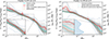 |
Fig. 1. Comparison between mean (solid red line), median (solid cyan line), and mode (dashed orange line) gas density profiles in two galaxy clusters (corresponding to the two panels). In addition to the standard mean profiles, mean profiles with masked substructures are shown by the dashed red lines. Light-grey lines indicate the individual directional profiles, while dotted cyan lines represent the (16−84)% percentiles at each r to give a better idea of the width of the density distribution. Dotted dark-blue lines indicate the thresholds for the substructure cleaning algorithm from which the dashed red line is obtained. The insets provide a zoomed-in view of two regions to highlight the differences among the profiles. The blue-filled line at the right of the right-hand panel inset depicts the density distribution at r ∼ 3Rvir, highlighting its bimodality. |
Focusing on CL101 (left-hand side panel), we show with grey lines the individual directional profiles, while the solid cyan (red) lines indicate the median (mean) radial profiles. For this comparison, mean profiles are computed as the arithmetic mean of Nθ × Nϕ = 25 × 25 directional profiles (instead of summing in a radial bin), so the problematics of finite-width shells are suppressed. There are three clearly distinct regions.
-
In the innermost regions (r/Rvir ≲ 0.04)5, mean profiles exceed median profiles by over a factor of 2 due to the very high-density tails reaching Δgas = ρgas/ρB > 107. This is not mitigated by the substructure-excised profiles (dashed red line, removing cells above 3.5σ in log ρ at each r; Zhuravleva et al. 2013) due to the broad density distribution (see the dashed dark-blue lines, indicating the thresholds for clump excision).
-
At intermediate radii (0.04 ≲ r/Rvir ≲ 1.5), where profiles tend to be more self-similar, the differences between the mean and median profiles are greatly reduced, with the exception of some bumps in the mean profile associated with prominent clumps that can be filtered out by the excision procedure. However, the inset presents a zoomed-in view showing how mean profiles overshoot the median one by (10 − 20)% even in this region of regularity.
-
In the outskirts (r/Rvir ≳ 1.5), mean and median profiles diverge again by almost an order of magnitude. In this region, besides the impact of clumping, the highly anisotropic environment drives mean densities up even if only a small portion of the solid angle points towards other overdense structures (filaments, other groups and clusters, etc.). In this sense, the median profiles are less sensitive to the anisotropy of the environment and suppress this two-halo contribution (Mo & White 1996; Sheth et al. 2001) more effectively.
The figures also show the mode profiles, i.e. the most likely value of gas density for each r, obtained from the directional profiles using a kernel density estimate (dashed orange line). This profile could arguably be the best representation of the smooth ICM and is robust under clumping. Our median profiles closely follow the mode profiles in the inner and intermediate region, where the former only exceed the latter by ∼5%.
The other cluster (CL126, right) follows similar patterns but exemplifies an important drawback of the mode profile, namely its behaviour in radial regions where the density probability distribution may not be monomodal. This is especially frequent in cluster outskirts. The inset shows a closer look at the 2 < r/Rvir < 3 radial range, where the density of grey lines (individual directional profiles) already hints at the presence of two regions of higher concentration. This is shown more clearly at the right of the inset, where we plot a histogram with the distribution of values of density, highlighting its bimodality. In such a scenario, mean profiles are dominated by the high-density region, while mode profiles are very unstable and may switch from one branch to the other depending on slight changes in the solid angle corresponding to a denser (e.g. filaments or a bridge with a nearby cluster) or a lower-density (i.e. voids) environment6. The considerations above lead us to choose the median profile as a conservative representation of the bulk, smooth component of the ICM for the remainder of this work.
3.2. Density profiles
We begin this section by analysing the effects of cluster assembly, quantified through the accretion rate at an aperture of R200m over the last dynamical time, Γ200m, as described in Sect. 2.1, on the radial mass distribution of clusters. We consider both baryonic and DM density profiles in the left and central panels of Fig. 2, respectively. Within each column, the upper panel displays the individual profiles as grey lines, while the red (green) lines with shaded regions correspond to the stacks over the lowest-accreting (highest-accreting) third of the population and their confidence regions7. Subsequent vertical panels in these figures highlight different aspects: the separation between stacked profiles of the two classes (second panel, showing the value of the class-stacked profiles normalised by the stack over the whole sample); the logarithmic derivative of the stacked profiles (third panel); and the partial Spearman rank correlation8 between the profile values at each r and accretion rate (fourth panel). With respect to this last one, it is worth noting that, throughout this work, we use these partial correlation coefficients to account for the dependences of the profiles on Γ that cannot be explained by the mass dependence of either the profiles (i.e. departures from self-similarity) or accretion rates.
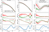 |
Fig. 2. Mass distribution for the highest accreting third (green) and lowest accreting third (red) of the sample. Left: Gas density. Center: DM density. Right: Baryon depletion. Top row: Profiles stacked over each subsample, together with the whole population (grey lines). Second row: Each class normalised by the ensemble average. Third row: Logarithmic slopes of the profiles, together with an indication of the radius of minimum slope. Bottom row: Correlation between the profiles and accretion rate Γ200m controlling for M200m. |
In cluster cores, there is a clear distinctive behaviour between gas and DM. On stacked profiles, low-accreting clusters prefer cuspy gas density profiles with logarithmic slopes consistent with ∼1 at ℛ ≡ r/R200m ∼ 0.01, while high-accreting clusters prefer cored profiles with slopes consistent with ∼0. This difference is not found on DM profiles, whose asymptotic inner slopes are ∼ − (0.2 − 0.3) regardless of Γ200m. On a cluster-by-cluster basis, this corresponds to a modest (but statistically significant) Spearman rank correlation of gas central density with accretion rate of ρsp ∼ −0.3, while for DM the correlation is consistent with being null (fourth row of Fig. 2). This is a consequence of the ability of intense accretion to offset the development of cool cores (Planelles & Quilis 2009; Hahn et al. 2017; Valdarnini & Sarazin 2021), while not impacting the central DM distribution – and hence suggesting that the offset must occur through increased pressure support (from compressive and turbulent heating), rather than just redistribution of mass by merger-induced advection.
Intermediate regions (0.1 ≲ ℛ ≲ 1) are, as often expected (Kravtsov & Borgani 2012), more self-similar, thus minimising the relative magnitude of the differences between our two classes. However, the Spearman rank correlations still reveal significant correlations: gas density is lower at ℛ ≲ 0.2 and higher at ℛ ≳ 0.2 as the accretion rate increases, likely as a consequence of gas being displaced outward to higher radii due to the offset of the cool core. Dark matter presents a different behaviour, its density being anti-correlated with the accretion rate up to ℛ ≲ 0.5 and being especially significant (|ρsp|∼0.5) within 0.1 ≲ ℛ ≲ 0.3.
Interestingly, Magnus et al. (2025) recover a similar correlation of gas density with Γ200m at intermediate radii to ours; however, this correlation also extends to DM in their study, at variance with our results here. Their analysis is, nevertheless, based on mean profiles, which are more sensitive to substructure and secondary haloes (this being precisely the effect that our median profiles are designed to suppress). We checked that repeating our analysis with mean profiles recovers a positive correlation between ρDM and Γ200m at intermediate radii, just as in our gas profiles and Magnus et al. (2025)’s DM profiles. This differential behaviour between the mean and median profiles of DM and gas indicates that gas undergoes a more coherent bulk displacement towards higher radii in response to intense accretion, whereas the DM profiles mainly reflect the localised influence of the secondary objects.
In the outskirts (ℛ > 1), the effects of accretion are better highlighted through the logarithmic slopes (third row of Fig. 2). In both cases, the radius of minimum (most negative) slope is larger for lower-accreting clusters. For DM profiles, this radius is usually associated with the splashback feature, generated by the accumulation of recently accreted particles in their first apocentric passage (Diemer et al. 2013; Adhikari et al. 2014). Its anti-correlation with accretion rates has been also highlighted in other studies (Diemer & Kravtsov 2014; O’Neil et al. 2021).
Interestingly, an analogous feature is observed for the gas density profiles, albeit at slightly larger radii. This has been interpreted by several authors as either a response of baryons to the splashback feature of DM or an indication of the accretion shock (O’Neil et al. 2021; Towler et al. 2024). Unlike Towler et al. (2024), we find that this feature does correlate with accretion rate, just as the splashback location does. However, we were unable to reconstruct this feature from hydrostatic equilibrium with the DM density profile alone. On the other hand, its radial location is inconsistent (too internal) to be a signature of the accretion shock. Indeed, the density jump of a strong shock is small (≲4) and could not fully account for the observed effect. Thus, although this feature must emerge as a transition from the one-halo to the two-halo (and intergalactic medium) regimes, its relation to the splashback feature or a shock is not straightforward and merits a detailed, separate study in the future.
The distinctive behaviour of the two components is reflected in the baryon depletion profile,
 (2)
(2)
presented in the right column of Fig. 2 for the standard radial profiles (solid lines) and for the cumulative profiles (Υ(< r), dashed lines). Assembly events being the only mechanism capable of offsetting over-cooling, dynamically active (relaxed) clusters present a clear under-abundance (overabundance) of gas with respect to the cosmic average in the region ℛ ≲ 0.1.
3.3. Thermodynamic profiles
We now turn to the analysis of temperature, entropy, and pressure profiles, as a summary of the thermodynamic state of the bulk ICM as described by our median profiles. These results are shown in Fig. 3 in an analogous way to Fig. 2.
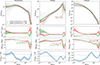 |
Fig. 3. Thermodynamic state of the highest-Γ200m third (green) and the lowest-Γ200m third (red) of the sample. Left: Temperature. Middle: Entropy. Right: Thermal pressure. The vertical panels within each column contain the same information as in Fig. 2. |
The left panel presents the temperature profiles for the lowest-accreting (red) and the highest-accreting (green) thirds. Clusters and groups with low accretion rates tend to be hotter–when normalised to their T200m–throughout the whole radial range, with an enhancement of their temperature profiles ranging from ∼30% at the core region (ℛ ≲ 0.04) to ∼10% at the intermediate, more self-similar radii. The separation of the logarithmic slopes is fairly limited out to ℛ ∼ 1, in such a way that the effect of high accretion on the temperature profiles mainly corresponds to a lower normalisation through the virial volume (as confirmed by the moderate, ρsp ∼ −0.3 anti-correlation). This might impact the integrated temperature and, thus, the TX − M scaling relation, as also seen for instance by Chen et al. (2019), or the LX − TX scaling (studied in relation to mergers by Planelles & Quilis 2009). However, we leave the impact of cluster assembly on the X-ray and SZ scaling relations for a future study.
In the case of entropy profiles (central column of Fig. 3), we instead observe a more complex pattern, where the entropy of strongly accreting clusters is consistently higher in the central regions (ℛ ≲ 0.1), while lower in the rest of the virial volume (0.1 ≲ ℛ ≲ 1). The former effect is consistent with the trends observed in the gas density (Sect. 3.2) and temperature profiles and confirms the ability of accretion to disturb cool cores. The entropy defect at intermediate radii may then be well explained by the merger-driven mixing with the lower-entropy central gas. In this regard, it is also worth discussing the presence of an important (∼25%) fraction of entropy cores among the individual profiles. We verified these to mostly correspond to objects in the high-Γ200m subsample, even though also a few low-Γ200m objects may display an entropy core. Reasons for this can be mainly due to our definition of accretion rate and aperture choices. For instance, a very tangential merger could increase Γ200m while having a delayed impact on the core; or, conversely, after a frontal merger that disrupts the core significantly, we could expect low (or even negative) accretion rates (e.g. Vallés-Pérez et al. 2020) if the infalling substructure reaches apocentric distances outside R200m.
Pressure profiles (right panel of Fig. 3) present their most salient dependence on accretion rate at the cluster centre, where the quotient between the low-Γ and the high-Γ central pressures reaches a factor of ∼4. In these central regions, this anti-correlation explains almost half of the scatter in the values of P/P200m, that is, in the departures of the central pressures from self-similarity. This trend is to be expected, since relaxed clusters are almost exclusively pressure-supported in their centres (e.g. XRISM Collaboration 2025a,b), while highly accreting systems tend to have higher central non-thermal pressures (Groth et al. 2025), as well as departures from hydrostatic equilibrium (Biffi et al. 2016; Angelinelli et al. 2020). Conversely, there is a slight but significant pressure enhancement in the highly accreting subsample in the region 0.3 ≲ ℛ ≲ 0.8, a feature similar to the one observed in the stacked SZ maps of Monllor-Berbegal et al. (2024).
Finally, it is instructive to consider the radii of steepest slope of these profiles, often associated with the location of the outermost accretion shock of groups and clusters (Shi 2016; Aung et al. 2021; Anbajagane et al. 2024; Zhang et al. 2025), even though care must be taken with this identification since the locations change significantly depending on the chosen variable. In general, in all cases (temperature, entropy, and pressure) we find a ∼10% decrease in the radial location of this feature for the higher-accreting objects with respect to the lower-accreting ones. A similar effect is observed with the location of the entropy peak, also often associated with the accretion shock radius (Lau et al. 2015; Zhang et al. 2025), albeit occurring at smaller radii. While the connection of these features to the accretion shock is far from trivial (even in a spherically averaged profile, it depends not only on the location but also on the underlying slope of the profile), we confirm a clear connection – in an ensemble-averaged sense – of high accretion rates being able to push inwards by ∼10% in radius the baryonic envelope of galaxy clusters and groups.
3.4. Dependence on individual assembly state indicators
As increasingly evident in recent literature, most of the quantities commonly used to assess the dynamical state of clusters are only loosely correlated among themselves (Jeeson-Daniel et al. 2011; Skibba & Macciò 2011; Haggar et al. 2020) and reflect different features or moments of the assembly history (Wong & Taylor 2012; Paper I). Therefore, it is interesting to examine which regions of the radial profile are better constrained by different assembly state indicators. We assess this on the entropy and the pressure profiles in Figs. 4 and 5, respectively, as two paradigmatic observables in X-ray and SZ. The set of indicators has been extracted from Paper I, to which we refer for more details on their definition, and contains the centre offset (Δr), virial ratio (η), mean radial velocity ( ), sparsity (s200c, 500c), ellipticity (ϵ), substructure fraction (fsub), Bullock et al. (2001) spin parameter (λBullock), and a combined indicator of relaxedness (χ; Vallés-Pérez et al. 2023, 2025b). These quantities are in all cases determined from the 3D description of the DM particle distribution and taking the virial radius as aperture. As some of them (Δr, ϵ) relate to the shape of the cluster, in Appendix C we consider a mock scenario to rule out that the dependencies we find here are purely geometric.
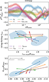 |
Fig. 4. Effect of individual indicators of assembly state on entropy profiles. Top: Spearman (partial) correlation coefficients of each indicator and profile values at each r/R200m. Higher magnitudes (either positive or negative) indicate a greater influence of the value of the indicator on the profile value at this particular radius. Middle: Effect of selecting clusters based on each parameter on the location and depth of the steepest logarithmic slope of the entropy profile. The crosses correspond to the profile stacked over the one-third most relaxed subsample (according to the given indicator), while the filled dots correspond to the most disturbed third. Bottom panel: Similar to the middle panel, but with the location and height of the entropy peak. The blue regions in the middle and bottom panels indicate the 68% confidence region for the determination of the corresponding locations over each of the Δr-based subsamples (as an example), obtained by bootstrap resampling. |
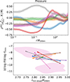 |
Fig. 5. Effect of individual indicators of assembly state on the pressure profiles. Top: Similar to that in Fig. 4, but with the pressure profiles. Bottom: Similar to the middle panel in Fig. 4, but with the pressure profiles. The colour code and other figure elements are kept the same as in the aforementioned figure. |
Looking at the entropy profiles, the top panel of Fig. 4 presents the correlation between each of the indicators and the normalised profile K(r)/K200m, controlling for the possible mass dependences. This quantity can be roughly interpreted as the fraction of the scatter in K(r)/K200m explained by each indicator. The rather intricate behaviour reflects the broad diversity of information brought up by different indicators. The central regions are better constrained by halo sparsity, with sparser haloes tending to have higher central entropies. At intermediate regions (0.1 ≲ ℛ ≲ 1) sparsity is instead anti-correlated with entropy, with halo spin and ellipticity following a very similar radial trend. By contrast, centre offset points in the opposite direction, the higher the offset, the higher the K(r)/K200m values. In this case, correlation coefficients are not high (reaching only |ρsp|∼0.4), indicating that, in addition to the effects that can be quantified by these indicators (mostly related to larger-scale assembly), other effects (e.g. radiative cooling) are crucial to set the entropy profile. However, it gives a clear account of the differential behaviour of subsamples built based on different indicators.
The effects of selecting clusters based on these assembly state indicators on the pressure profile (top panel of Fig. 5) are stronger, especially in the central regions (ℛ < 0.2), where sparsity reaches anti-correlations |ρsp|∼0.5 − 0.7, thus explaining much of the variability in the deviations from self-similarity in the profiles. Driven by this indicator, the combination χ also achieves high (ρsp ∼ 0.5) correlations in this range. At larger radii ℛ ∈ [0.1, 1], also centre offset anti-correlates significantly with the pressure profile, while the effect of other indicators at intermediate and outer radii is limited.
Finally, to study cluster outskirts, it is interesting to look at the effect of building samples selected on these parameters on the singular radii studied in Sect. 3.3. The second panel of Figs. 4 and 5 show, respectively, how the location and the value of the logarithmic slope minima of the entropy and pressure profiles change from the most-relaxed (crosses) to the most-disturbed (circles) third of the sample according to each indicator. In both cases, the effect of increasing most of the parameters (Δr, η, fsub, etc.) is to push the radius of steepest slope inwards, as strongly accreting clusters tend to have slightly less extended atmospheres. However, λBullock and s200c, 500c tend to point in the vertical direction, i.e. disturbed objects have a shallower steepening in their outskirts (probably associated with a more aspherical accretion shock shell). The third panel of Fig. 4 does the same with the location and value of the entropy peak, which largely mirror the trends seen for the steepest slopes. In all cases, the exception is the mean radial velocity magnitude, which points in the opposite direction, with high  clusters having more extended atmospheres. This odd behaviour can be attributed to a couple of factors: (i)
  is sign-degenerate by construction, meaning that both strong inflows and outflows drive up its value, thus potentially mixing timescales; (ii) as shown by Paper I, it is a very instantaneous indicator, whereas the response of the accretion shock to mergers is a slow process that takes well over a dynamical time.
3.5. Scatter around the profiles
So far, we have examined the radial profile trends in connection to cluster assembly. A further, key aspect is the scatter around these trends, arising from departures from spherical symmetry.
In the first panel of Fig. 6, we show the asphericity of the profiles. We define, for a given quantity X, its asphericity as
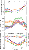 |
Fig. 6. Deviations from sphericity and self-similarity of cluster profiles. Top: ICM asphericity, 𝒜(r), profiles for different quantities. Middle: Spearman rank correlation of profile asphericity with accretion rates. Bottom: Departure from self-similarity, 𝒮(x), of the profiles. The dashed lines correspond to the quotient of this quantity among the highest- and lowest-accreting thirds of the sample. |
 (3)
(3)
with Xp% being the p-th percentile of the values of X at radius r; namely, 𝒜X(x) is a measure of the logarithmic width of the distribution of X(Ω | r), Ω denoting solid angle. Generally, all gas profiles (T, K, P, and ρgas) exhibit similar features, with intermediate radii (0.1 ≲ ℛ ≲ 1) being the most spherical and asphericity increasing both towards the centre and the outskirts of the ICM. The latter reflects the increasing anisotropy of the environment, whereas the former likely arises from the complex morphology of cooling flows. These flows are likely to be modified by active galactic nuclei (AGN) feedback. Nonetheless, detailed simulations show how gaseous morphology remains complex in the vicinity of AGN (Quilis et al. 2001; Teyssier et al. 2011; Gaspari et al. 2012). Moreover, although all thermodynamic quantities present broadly similar radial trends, the maximum sphericity (lowest 𝒜X(r)) is achieved at slightly different radii, ranging from ℛ ∼ 0.05 for P(r), to ℛ ∼ 0.2 for K(r). Conversely, the DM density anisotropy monotonically increases with radius, thus being most spherical in the centre. This discrepant behaviour is explained by the collisionless nature of DM, where higher densities imply more frequent gravitational collisions (i.e. violent relaxation, collisionless mixing; Lynden-Bell 1967; Binney & Tremaine 1987), and a randomisation of particle orbits (e.g. Navarro et al. 2010).
Of interest here is how the asphericity of DM and ICM profiles depends on accretion rates, shown in the second panel of Fig. 6 in a similarly way as in the bottom panels of Figs. 2 and 3. Notably, although correlations are weak (|ρsp|∼0.2) in the core region, DM density asphericity correlates with accretion rate, while it anti-correlates for the gaseous profiles. This implies that ∼20% of the variability in the asphericity of central DM densities is explained by the virial mass increase over the last dynamical time, while clusters that have undergone higher accretion tend to display, somewhat surprisingly, slightly more spherical innermost gaseous distribution. The trend, albeit weak, can be attributed to mergers inducing subsonic turbulence on τdyn timescales (Vazza et al. 2017; Vallés-Pérez et al. 2021), which in turn mixes and homogenises the baryonic distribution (e.g. Lau et al. 2011); as well as to the emergence of morphologically complex cooling flows in very relaxed cluster cores. In the intermediate region, we mildly recover the expected behaviour, where the higher the accretion rates, the more aspherical the ICM becomes. This effect is observed for both DM and gas properties, but especially for the temperature profile (which, moreover, tends to be the most spherically symmetric). The correlations are mild, probably because merging events (which largely determine Γ200m) tend to impact the tails of the baryonic distributions (beyond the 84% percentile) and may be not captured by our definition in Eq. (3), which focuses on the asphericity of the smooth ICM. As a matter of fact, Vazza et al. (2011) and Eckert et al. (2012) do recover correlations between dynamical state or cool-coredness (respectively) and scatter around the profiles, likely as a consequence of their definition of the scatter (computed directly from a standard deviation with a suitable masking of outliers), which is more sensitive to extreme values.
Finally, in the third panel of Fig. 6 we assess the level of departure from self-similarity of the profiles, quantified in a similar way to asphericity as
 (4)
(4)
where the notation {𝒳(r)}p% denotes the p-th percentile (over the whole cluster sample) of the values of the median profiles X(r), each normalised by their self-similar value Xnorm (see Sect. 2.3). As widely discussed in the literature (e.g. Ghirardini et al. 2019), both DM and gaseous profiles are most self-similar at intermediate radii (roughly [0.2 − 0.8]R200m for all quantities considered here). The exception is, perhaps, the entropy profile, whose most self-similar region extends almost up to the accretion shock (∼2R200m), in line with its most spherically symmetric region located further out.
In the literature (Pratt et al. 2009; Lovisari et al. 2015), it is generally observed that relaxed clusters (according to any suitable criterion) behave more self-similarly. To check this, we show, as the dashed lines, the quotient between these departures from self-similarity, 𝒮X(r), between the highest-accreting third and the lowest-accreting third. These quotients are close to unity, perhaps with the exception of temperature, which is slightly above 1 throughout the whole radial range. The fact that we do not see broader cluster-to-cluster variance in the median profiles of highly accreting clusters points in the direction of recent literature (Ghirardini et al. 2022; Vallés-Pérez et al. 2023; Haggar et al. 2024), in suggesting that there is not a bimodality between disturbed and relaxed clusters, but rather only some –moderate– continuous trends of the profiles with assembly state.
3.6. Fits to standard functional forms
We now shift from the non-parametric profile analyses to the impact of accretion on the parameters of standard fitting formulae. To do so, we split our complete sample at z = 0 into ten equal-sized accretion-rate bins, separated by the deciles in Γ200m. All fits were performed using a Markov chain Monte Carlo (MCMC) method. Full details of the fitting procedure and the explicit functional forms are provided in Appendix D.
3.6.1. NFW concentration
Fig. 7 shows how the concentration c200m of the DM (red) and gas (blue) density profiles change with the accretion intensity over the last dynamical time, assuming a Navarro et al. (1997, NFW) functional form (Eq. D.1). For the DM profile, we find no strong trend of c200m with Γ200m, partly at odds with recent bibliography (Wechsler et al. 2002; Wang et al. 2020) who suggest that this quantity is driven by major mergers. However, this is not surprising, since Giocoli et al. (2012) showed how c200m depends non-trivially on matter accretion over a combination of timescales. Conversely, for the gas density profiles we observe a strong anti-correlation9, such that the larger the accretion rate over the last τdyn, the smaller the concentration parameter (i.e. the larger the scale radius). Both these results are consistent with the findings of Sect. 3.2, where we observed a clear trend for the central gas density profiles (related to the ability of accretion to offset over-cooling), while there is no appreciable difference in the DM density slopes.
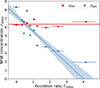 |
Fig. 7. Concentration c200m = R200m/rs (with rs being the best-fit scale radius of the NFW functional form) of the DM (red), and gas (blue) profiles stacked in deciles of accretion rate Γ200m over the last dynamical time. The dots indicate the results for each decile of accretion rate, with 1σ error bars, while the lines show linear fits with their confidence regions. |
Overall, we find that DM and gas concentrations in our sample can be well described by
 (5)
(5)
 (6)
(6)
3.6.2. gNFW slopes
Now assuming a generalised NFW (gNFW, Eq. D.2), we show in Fig. 8 the effect of accretion on the internal (α) and external (β) slopes, and the transition sharpness (γ), for the DM density (red), gas density (blue), and the pressure profile (green).
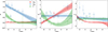 |
Fig. 8. Dependence of the inner slope (α, left), the outer slope (β, middle), and the transition parameter (γ, right) of a gNFW model on the accretion rate, for the DM density (red), gas density (blue), and pressure (green) profiles. Dots with error bars represent the results from the fit to the profiles stacked over each decile in Γ200m. The lines represent least-squares polynomial fits, with the dark-shaded regions showing the fit uncertainty, and the light-shaded regions also including the uncertainty of the dots added in quadrature (assuming it depends linearly on Γ200m). |
Regarding internal slopes, consistently with the findings in Sect. 3.2, clusters experiencing low accretion develop very steep gas density cusps (α ∼ 2), which progressively flatten as Γ200m increases. The same is not observed for DM profiles, which are consistent with flat cores regardless of accretion rate (possibly partly contributed by mass resolution). Combining this with the central temperature decrease in disturbed clusters, shown in Sect. 3.3, pressure profiles exhibit an almost bimodal behaviour, with weak cusps α ≃ 0.75 for Γ200m ≲ 0.5, and flat cores otherwise. An indication of this was also observed by Monllor-Berbegal et al. (2024) for the thermal SZ signal.
External slopes of the median profiles (which, as discussed in Sect. 3.2, represent the one-halo term and tend to be steeper than the β = 3 NFW value) show clear dependence on accretion rate. For DM densities, the most relaxed clusters and groups are consistent or only marginally above the NFW value, respectively. However, as accretion rates increase, the outer gNFW slopes get increasingly steeper, even reaching β ≳ 6 for Γ200m ∼ 4. This does not imply that the outer slopes actually reach dlog ρDM/dlog r = −6 (see Fig. 2), as β only represents the slope at r → ∞; but this result emerges as a combination of (i) larger scale radii while measured outer slopes (see Fig. 2) remain similar, and (ii) smaller splashback radii, that truncate the one-halo term earlier and thus make the outskirts slightly steeper. Interestingly, the outer slope of the pressure profile varies in the opposite way, with shallower outer slopes for highly accreting clusters, which again is not observed in the third panel on the right of Fig. 3. Overall, these trends warn us about the meaning of gNFW parameters, which are highly correlated, when describing the ICM and DM halo structure.
Finally, the parameter controlling the sharpness of the transition (γ) only presents a noticeable dependence on Γ200m for the case of the DM profile, where the transition is smoothed out (lower γ) for higher-accreting clusters, as a consequence of the loss of sphericity. This trend is much weaker or almost non-existent for the ICM, probably because this medium is already much more spherical due to its collisional nature.
3.6.3. Entropy profiles
Lastly, we turn our attention to the entropy profiles, which we fitted to the Donahue et al. (2006) and Cavagnolo et al. (2009) model (Eq. D.3) consisting of a power law (with normalisation K0.1 at r = 0.1R200m and slope α) plus an entropy core (K0). To mitigate the effects of over-cooling on the results, we restricted the fits to the interval r ∈ [0.1, 2]R200m. We show the dependence of K0 and K0.1 (red and blue lines, respectively, in units of K200m) on Γ200m in the upper panel of Fig. 9.
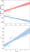 |
Fig. 9. Variation of the core excess entropy (K0, red line in the upper panel), power-law normalisation (K0.1, blue line in the upper panel) and power-law index (lower panel) with accretion rate. All plot elements are equivalent to those in Fig. 8. |
Entropy floor values present an approximately monotonic increase with Γ200m, from values of K0 ≈ 0.12K200m to K0 ≈ 0.2K200m when varying from the lowest accreting to the highest accreting deciles. This increase in the core excess, which is a direct manifestation of the role of gas accretion – mainly through mergers – in offsetting cool cores (Poole et al. 2006, 2008; Planelles & Quilis 2009; Zinger et al. 2016; Valdarnini & Sarazin 2021) is compensated by decreasing normalisation in the power-law range, K0.1. Additionally, we observe a steepening of the entropy profiles. For relaxed clusters, we find a slope α ≈ 1.25 slightly larger than the reference value α ≈ 1.1 (Voit et al. 2005), as expected since cooling times decrease with increasing density and dense gas over-cools faster. This slope increases with Γ200m reaching values around α ≈ 1.5 for clusters with Γ200m ≳ 1. Interestingly, these do not seem to follow a continuous trend, but rather a step around Γ200m ∼ 1.
4. Discussion and conclusions
Building upon cutting-edge X-ray (EROSITA, Merloni et al. 2024; CHEX-MATE, CHEX-MATE Collaboration 2021) and SZ observational campaigns (e.g. ACT, ACTDESHSC Collaboration 2025), next-generation observatories (NEWATHENA, Cruise et al. 2025; SIMONS OBSERVATORY, Abitbol et al. 2025) will provide deeper constraints on ICM thermodynamics, increasing sample size, redshift coverage, and radial apertures. Given the complexity of the physical processing that set the thermodynamic state of the ICM, it is instructive to study how far the assembly of the cluster itself – setting aside internal processes due to galactic physics – conditions its internal structure. In this work, we aimed to address this issue by studying the radial median profiles of DM and ICM properties for a sample of simulated clusters and groups at z = 0, spanning masses from 1013 M⊙ to ∼7 × 10¹⁴ M⊙, where only cooling – but no feedback processes – is included besides pure hydrodynamics and gravity. In this way, we isolated the effects of gravitational heating, while deferring the assessment of the impact of feedback to a future study. We summarise our main conclusions below, placing them in the context of recent literature:
-
Radial median profiles provide a sound representation of the bulk ICM, largely insensitive to the presence of substructure and clumps without the need for artificial thresholds (e.g. Zhuravleva et al. 2013), and are insensitive to shot noise independently of binning choices if computed as detailed in Sect. 2.2. These profiles largely match the mode profiles – which arguably trace the most typical ICM state at a given r – while being more robust under larger-scale anisotropy in the outskirts. While the common practice in simulations is to take mean profiles with ad hoc substructure excision processes, we argue that the technique used in this work is also desirable due to its consistency with the azimuthal median technique in observational data (Eckert et al. 2015).
-
Accretion affects DM and gas density profiles differently. Central gas is reduced by a factor of up to 4 between the lowest and highest accreting subsamples, effectively transforming strong cusps into flat cores. However, DM central densities are not significantly affected by accretion. This partly contrasts with Lau et al. (2015), who reported that the inner gas density slopes remain unaffected by accretion (their Fig. 8b), likely due to their non-radiative set-up. At intermediate radii (0.1 ≲ r/R200m ≲ 1), highly accreting clusters tend to have their gas content displaced outward to higher radii.
-
Central temperatures do not strongly vary with accretion rate, but their normalisation at intermediate radii decreases by ∼10% for the highly accreting subsample. Entropy profiles, in turn, do exhibit a clear central increase for highly accreting clusters, as the central gas mixes more effectively with the higher-entropy surroundings. Consistently, at intermediate radii, there is a ∼(10 − 20)% decrease in the entropy of disturbed clusters. Lastly, pressure profiles reveal their strongest dependence on accretion in the centre, up to a factor of ∼4 between the two extreme classes (as also found for thermal SZ profiles, for instance by Monllor-Berbegal et al. 2024). In general, these trends were not captured by the analyses of Lau et al. (2015), most likely because the absence of cooling prevents the buildup of dense and cold central gas, which accretion would otherwise reheat.
-
In the outskirts, high accretion shifts the radii of steepest slope (for both ρDM and ρgas) inwards. This result had already been found for the ρDM, where this steepest slope roughly corresponds to the splashback feature (e.g. More et al. 2015; Shin & Diemer 2023). For the thermodynamic profiles (temperature, entropy, and pressure profiles), the radius of steepest slope responds to the average location of the accretion shock. It does shrink – albeit to a smaller extent than Rsp (∼10%) – with increasing accretion rate, as expected from theoretical considerations (Shi 2016) and also reported by Aung et al. (2021) and Zhang et al. (2025).
-
Selection of clusters based on indicators of assembly state bears a non-trivial effect on the profiles (Figs. 4 and 5). For instance, while entropy in the 0.1R200m ≲ r ≲ R200m range moderately anti-correlates with sparsity, it positively correlates with centre offset, despite both s200c, 500c and Δr being a measure of dynamical unrelaxation. Moreover, the correlations do not tend to be strong (in line with, e.g. Lau et al. 2021, their Fig. 4). These quantities, insofar as they are proxies for the halo and ICM mass growth, carry an imprint on the characteristic outermost radii delimiting the extent of the ICM (entropy peak, steepest slopes). In general, less relaxed clusters (according to any indicator) exhibit smaller baryonic boundaries by up to ∼10%. However, other quantities (e.g. Δr or λBullock) are more indicative of the sharpness of the features, suggesting that they are predictive of the sphericity of the accretion shock.
-
Departures from sphericity in the baryonic profiles are minimum at intermediate (0.1R200m ≲ r ≲ R200m) radii – where the profiles are also more self-similar – and increase both towards the core and the outskirts due to complex cooling flow morphologies and environmental anisotropy, respectively. In contrast, DM density is most spherical at the centre. Correlations of asphericity with accretion rates over the last dynamical time are rather weak, as a result of a combination of physical effects and our definition of asphericity, perhaps with the clearest signal on the temperature profile at intermediate radii. Examining intrinsic scatter over the cluster population, we recover the trends observed by Ghirardini et al. (2019) on the X-COP sample, namely a log-parabolic trend for the scatter, with temperature and pressure profiles respectively behaving as the most and the least self-similar quantity.
-
When profiles are stacked on deciles of Γ200m, we see clear signatures of accretion on the estimation of parameters from widely used functional forms. In particular, the concentration of a NFW model fitted to gas density reveals a strong dependence of c200m on Γ200m, while the same does not occur for the DM density profiles. This might be the case because the value of concentration of the gaseous profile depends on the emergence of a cusp driven by (over)cooling; while in the case of DM concentration, it has been reported how it depends non-trivially on the combination of several timescales (Giocoli et al. 2012). When leaving the slopes as free parameters (gNFW), we recover a tendency for gas to develop strong cusps (α ≃ 1.5) in the absence of accretion, which are progressively transformed into cores at high accretion rates. External slopes, especially in the case of DM density, exhibit a strong dependence on accretion rates, with sharper truncations for higher-accreting objects. Entropy profiles adhere to the Cavagnolo et al. (2009) form only within 0.1R200m ≲ r ≲ 2R200m, with a clear indication of the offset of cool cores by strong accretion.
Several limitations of the present analysis should be kept in mind. While the simulation set-up employed here is ideal for isolating gravitational heating on the ICM, future work will need to incorporate its complex interplay with stellar and AGN feedback at group and cluster scales, which are key to obtaining ICM distributions consistent with observations (McNamara & Nulsen 2012; Fabian 2012; Planelles et al. 2014), especially in the innermost regions. A second caveat concerns our assumption of self-similar scaling to stack the profiles. A number of recent studies (Pratt et al. 2010; Riva et al. 2024) have highlighted that allowing for substantial deviations from the theoretical (Kaiser 1986) self-similar scaling with mass results in a reduced intrinsic scatter around the profiles. Although we do not address this here due to space and scope limitations, it remains a key issue and represents an important direction for future work. Finally, assessing to what extent the trends identified in our 3D profiles remain in projection is of high interest. Advancing along these lines will be essential to extract the maximum information from current and future observational surveys of the thermal ICM.
Acknowledgments
We are grateful to Annalisa Bonafede and to the anonymous reviewer for their careful reading of this manuscript and valuable suggestions, and to Franco Vazza and Marco Balboni for insightful discussions about this work. This work has been supported by the Agencia Estatal de Investigación Española (AEI; grant PID2022-138855NB-C33), by the Ministerio de Ciencia e Innovación (MCIN) within the Plan de Recuperación, Transformación y Resiliencia del Gobierno de España through the project ASFAE/2022/001, with funding from European Union NextGenerationEU (PRTR-C17.I1), and by the Generalitat Valenciana (grant CIPROM/2022/49). DVP acknowledges partial support from Universitat de València through an Atracció de Talent fellowship. The simulation and part of the analysis have been carried out using the supercomputer Lluís Vives at the Servei d’Informótica of the Universitat de València. This research has been made possible by the following open-source projects: Numpy (Harris et al. 2020), Scipy (Virtanen et al. 2020), Matplotlib (Hunter 2007), FFTW (Frigo & Johnson 2005), emcee (Foreman-Mackey et al. 2013).
References
- Abitbol, M., Abril-Cabezas, I., Adachi, S., et al. 2025, JCAP, 2025, 034 [Google Scholar]
- ACTDESHSC Collaboration (Aguena, M., et al.) 2025, ArXiv e-prints [arXiv:2507.21459] [Google Scholar]
- Adhikari, S., Dalal, N., & Chamberlain, R. T. 2014, JCAP, 2014, 019 [Google Scholar]
- Anbajagane, D., Chang, C., Baxter, E. J., et al. 2024, MNRAS, 527, 9378 [Google Scholar]
- Angelinelli, M., Vazza, F., Giocoli, C., et al. 2020, MNRAS, 495, 864 [NASA ADS] [CrossRef] [Google Scholar]
- Angelinelli, M., Ettori, S., Vazza, F., & Jones, T. W. 2021, A&A, 653, A171 [NASA ADS] [CrossRef] [EDP Sciences] [Google Scholar]
- Angelinelli, M., Ettori, S., Dolag, K., Vazza, F., & Ragagnin, A. 2022, A&A, 663, L6 [NASA ADS] [CrossRef] [EDP Sciences] [Google Scholar]
- Ansarifard, S., Rasia, E., Biffi, V., et al. 2020, A&A, 634, A113 [NASA ADS] [CrossRef] [EDP Sciences] [Google Scholar]
- Arnaud, M., Pointecouteau, E., & Pratt, G. W. 2005, A&A, 441, 893 [NASA ADS] [CrossRef] [EDP Sciences] [Google Scholar]
- Aung, H., Nagai, D., & Lau, E. T. 2021, MNRAS, 508, 2071 [NASA ADS] [CrossRef] [Google Scholar]
- Battaglia, N., Bond, J. R., Pfrommer, C., & Sievers, J. L. 2013, ApJ, 777, 123 [NASA ADS] [CrossRef] [Google Scholar]
- Beers, T. C., Flynn, K., & Gebhardt, K. 1990, AJ, 100, 32 [Google Scholar]
- Biffi, V., Dolag, K., & Böhringer, H. 2013, MNRAS, 428, 1395 [Google Scholar]
- Biffi, V., Borgani, S., Murante, G., et al. 2016, ApJ, 827, 112 [NASA ADS] [CrossRef] [Google Scholar]
- Binney, J., & Tremaine, S. 1987, Galactic Dynamics (Princeton: Princeton University Press) [Google Scholar]
- Böhringer, H., & Werner, N. 2010, A&ARv, 18, 127 [Google Scholar]
- Borgani, S., Murante, G., Springel, V., et al. 2004, MNRAS, 348, 1078 [Google Scholar]
- Bryan, G. L., & Norman, M. L. 1998, ApJ, 495, 80 [NASA ADS] [CrossRef] [Google Scholar]
- Bullock, J. S., Kolatt, T. S., Sigad, Y., et al. 2001, MNRAS, 321, 559 [Google Scholar]
- Cavagnolo, K. W., Donahue, M., Voit, G. M., & Sun, M. 2009, ApJS, 182, 12 [Google Scholar]
- Chen, H., Avestruz, C., Kravtsov, A. V., Lau, E. T., & Nagai, D. 2019, MNRAS, 490, 2380 [NASA ADS] [CrossRef] [Google Scholar]
- CHEX-MATE Collaboration (Arnaud, M., et al.) 2021, A&A, 650, A104 [NASA ADS] [CrossRef] [EDP Sciences] [Google Scholar]
- Cramer, H. 1946, Mathematical Methods of Statistics (Princeton: Princeton University Press) [Google Scholar]
- Cruise, M., Guainazzi, M., Aird, J., et al. 2025, Nat. Astron., 9, 36 [Google Scholar]
- Davé, R., Cen, R., Ostriker, J. P., et al. 2001, ApJ, 552, 473 [Google Scholar]
- De Luca, F., De Petris, M., Yepes, G., et al. 2021, MNRAS, 504, 5383 [NASA ADS] [CrossRef] [Google Scholar]
- Diemer, B., & Kravtsov, A. V. 2014, ApJ, 789, 1 [NASA ADS] [CrossRef] [Google Scholar]
- Diemer, B., More, S., & Kravtsov, A. V. 2013, ApJ, 766, 25 [NASA ADS] [CrossRef] [Google Scholar]
- Dolag, K., Vazza, F., Brunetti, G., & Tormen, G. 2005, MNRAS, 364, 753 [NASA ADS] [CrossRef] [Google Scholar]
- Donahue, M., Horner, D. J., Cavagnolo, K. W., & Voit, G. M. 2006, ApJ, 643, 730 [NASA ADS] [CrossRef] [Google Scholar]
- Eckert, D., Vazza, F., Ettori, S., et al. 2012, A&A, 541, A57 [NASA ADS] [CrossRef] [EDP Sciences] [Google Scholar]
- Eckert, D., Roncarelli, M., Ettori, S., et al. 2015, MNRAS, 447, 2198 [Google Scholar]
- Eckert, D., Ghirardini, V., Ettori, S., et al. 2019, A&A, 621, A40 [NASA ADS] [CrossRef] [EDP Sciences] [Google Scholar]
- Evrard, A. E. 1990, ApJ, 363, 349 [NASA ADS] [CrossRef] [Google Scholar]
- Fabian, A. C. 2012, ARA&A, 50, 455 [Google Scholar]
- Foreman-Mackey, D., Hogg, D. W., Lang, D., & Goodman, J. 2013, PASP, 125, 306 [Google Scholar]
- Frigo, M., & Johnson, S. G. 2005, Proc. IEEE, 93, 216 [Google Scholar]
- Gaspari, M., Ruszkowski, M., & Sharma, P. 2012, ApJ, 746, 94 [Google Scholar]
- Ghirardini, V., Eckert, D., Ettori, S., et al. 2019, A&A, 621, A41 [NASA ADS] [CrossRef] [EDP Sciences] [Google Scholar]
- Ghirardini, V., Bahar, Y. E., Bulbul, E., et al. 2022, A&A, 661, A12 [NASA ADS] [CrossRef] [EDP Sciences] [Google Scholar]
- Giocoli, C., Tormen, G., & Sheth, R. K. 2012, MNRAS, 422, 185 [NASA ADS] [CrossRef] [Google Scholar]
- Groth, F., Valentini, M., Steinwandel, U. P., Vallés-Pérez, D., & Dolag, K. 2025, A&A, 693, A263 [NASA ADS] [CrossRef] [EDP Sciences] [Google Scholar]
- Haggar, R., Gray, M. E., Pearce, F. R., et al. 2020, MNRAS, 492, 6074 [NASA ADS] [CrossRef] [Google Scholar]
- Haggar, R., De Luca, F., De Petris, M., et al. 2024, MNRAS, 532, 1031 [Google Scholar]
- Hahn, O., Martizzi, D., Wu, H.-Y., et al. 2017, MNRAS, 470, 166 [NASA ADS] [Google Scholar]
- Harris, C. R., Millman, K. J., van der Walt, S. J., et al. 2020, Nature, 585, 357 [NASA ADS] [CrossRef] [Google Scholar]
- Hernández-Martínez, E., Dolag, K., Steinwandel, U. P., et al. 2025, A&A, submitted [arXiv:2507.15858] [Google Scholar]
- Hunter, J. D. 2007, Comput. Sci. Eng., 9, 90 [NASA ADS] [CrossRef] [Google Scholar]
- Jeeson-Daniel, A., Dalla Vecchia, C., Haas, M. R., & Schaye, J. 2011, MNRAS, 415, L69 [NASA ADS] [Google Scholar]
- Kaiser, N. 1986, MNRAS, 222, 323 [Google Scholar]
- Knebe, A., Knollmann, S. R., Muldrew, S. I., et al. 2011, MNRAS, 415, 2293 [Google Scholar]
- Kravtsov, A. V., & Borgani, S. 2012, ARA&A, 50, 353 [Google Scholar]
- Kuchner, U., Aragón-Salamanca, A., Pearce, F. R., et al. 2020, MNRAS, 494, 5473 [NASA ADS] [CrossRef] [Google Scholar]
- Lau, E. T., Nagai, D., Kravtsov, A. V., & Zentner, A. R. 2011, ApJ, 734, 93 [CrossRef] [Google Scholar]
- Lau, E. T., Nagai, D., Avestruz, C., Nelson, K., & Vikhlinin, A. 2015, ApJ, 806, 68 [NASA ADS] [CrossRef] [Google Scholar]
- Lau, E. T., Hearin, A. P., Nagai, D., & Cappelluti, N. 2021, MNRAS, 500, 1029 [Google Scholar]
- Le Brun, A. M. C., McCarthy, I. G., Schaye, J., & Ponman, T. J. 2014, MNRAS, 441, 1270 [NASA ADS] [CrossRef] [Google Scholar]
- Lovisari, L., Reiprich, T. H., & Schellenberger, G. 2015, A&A, 573, A118 [NASA ADS] [CrossRef] [EDP Sciences] [Google Scholar]
- Lynden-Bell, D. 1967, MNRAS, 136, 101 [Google Scholar]
- Magnus, L. C., Kay, S. T., Schaye, J., & Schaller, M. 2025, MNRAS, 545, 14 [Google Scholar]
- Marini, I., Popesso, P., Dolag, K., et al. 2025, A&A, 698, A191 [NASA ADS] [CrossRef] [EDP Sciences] [Google Scholar]
- McNamara, B. R., & Nulsen, P. E. J. 2007, ARA&A, 45, 117 [NASA ADS] [CrossRef] [Google Scholar]
- McNamara, B. R., & Nulsen, P. E. J. 2012, New J. Phys., 14, 055023 [NASA ADS] [CrossRef] [Google Scholar]
- Merloni, A., Lamer, G., Liu, T., et al. 2024, A&A, 682, A34 [NASA ADS] [CrossRef] [EDP Sciences] [Google Scholar]
- Mo, H. J., & White, S. D. M. 1996, MNRAS, 282, 347 [Google Scholar]
- Monllor-Berbegal, Ó., Vallés-Pérez, D., Planelles, S., & Quilis, V. 2024, A&A, 686, A243 [NASA ADS] [CrossRef] [EDP Sciences] [Google Scholar]
- More, S., Diemer, B., & Kravtsov, A. V. 2015, ApJ, 810, 36 [Google Scholar]
- Mroczkowski, T., Nagai, D., Basu, K., et al. 2019, Space Sci. Rev., 215, 17 [Google Scholar]
- Navarro, J. F., Frenk, C. S., & White, S. D. M. 1997, ApJ, 490, 493 [Google Scholar]
- Navarro, J. F., Ludlow, A., Springel, V., et al. 2010, MNRAS, 402, 21 [Google Scholar]
- O’Neil, S., Barnes, D. J., Vogelsberger, M., & Diemer, B. 2021, MNRAS, 504, 4649 [CrossRef] [Google Scholar]
- Planck Collaboration VI. 2020, A&A, 641, A6 [NASA ADS] [CrossRef] [EDP Sciences] [Google Scholar]
- Planelles, S., & Quilis, V. 2009, MNRAS, 399, 410 [NASA ADS] [CrossRef] [Google Scholar]
- Planelles, S., & Quilis, V. 2010, A&A, 519, A94 [NASA ADS] [CrossRef] [EDP Sciences] [Google Scholar]
- Planelles, S., Borgani, S., Dolag, K., et al. 2013, MNRAS, 431, 1487 [Google Scholar]
- Planelles, S., Borgani, S., Fabjan, D., et al. 2014, MNRAS, 438, 195 [Google Scholar]
- Planelles, S., Schleicher, D. R. G., & Bykov, A. M. 2015, Space Sci. Rev., 188, 93 [NASA ADS] [CrossRef] [Google Scholar]
- Planelles, S., Fabjan, D., Borgani, S., et al. 2017, MNRAS, 467, 3827 [Google Scholar]
- Poole, G. B., Fardal, M. A., Babul, A., et al. 2006, MNRAS, 373, 881 [Google Scholar]
- Poole, G. B., Babul, A., McCarthy, I. G., Sanderson, A. J. R., & Fardal, M. A. 2008, MNRAS, 391, 1163 [CrossRef] [Google Scholar]
- Pratt, G. W., Croston, J. H., Arnaud, M., & Böhringer, H. 2009, A&A, 498, 361 [NASA ADS] [CrossRef] [EDP Sciences] [Google Scholar]
- Pratt, G. W., Arnaud, M., Piffaretti, R., et al. 2010, A&A, 511, A85 [NASA ADS] [CrossRef] [EDP Sciences] [Google Scholar]
- Quilis, V. 2004, MNRAS, 352, 1426 [NASA ADS] [CrossRef] [Google Scholar]
- Quilis, V., M, J., Ibáñez, & Sáez, D. 1998, ApJ, 502, 518 [Google Scholar]
- Quilis, V., Bower, R. G., & Balogh, M. L. 2001, MNRAS, 328, 1091 [NASA ADS] [CrossRef] [Google Scholar]
- Rasia, E., Tripodi, R., Borgani, S., et al. 2025, A&A, 702, A182 [NASA ADS] [CrossRef] [EDP Sciences] [Google Scholar]
- Riva, G., Pratt, G. W., Rossetti, M., et al. 2024, A&A, 691, A340 [NASA ADS] [CrossRef] [EDP Sciences] [Google Scholar]
- Savitzky, A., & Golay, M. J. E. 1964, Anal. Chem., 36, 1627 [Google Scholar]
- Sheth, R. K., Hui, L., Diaferio, A., & Scoccimarro, R. 2001, MNRAS, 325, 1288 [Google Scholar]
- Shi, X. 2016, MNRAS, 461, 1804 [NASA ADS] [CrossRef] [Google Scholar]
- Shin, T.-H., & Diemer, B. 2023, MNRAS, 521, 5570 [NASA ADS] [CrossRef] [Google Scholar]
- Skibba, R. A., & Macciò, A. V. 2011, MNRAS, 416, 2388 [NASA ADS] [CrossRef] [Google Scholar]
- Sunyaev, R. A., & Zeldovich, Y. B. 1972, Comments Astrophys. Space Phys., 4, 173 [NASA ADS] [EDP Sciences] [Google Scholar]
- Teyssier, R., Moore, B., Martizzi, D., Dubois, Y., & Mayer, L. 2011, MNRAS, 414, 195 [NASA ADS] [CrossRef] [Google Scholar]
- Towler, I., Kay, S. T., & Altamura, E. 2023, MNRAS, 520, 5845 [NASA ADS] [CrossRef] [Google Scholar]
- Towler, I., Kay, S. T., Schaye, J., et al. 2024, MNRAS, 529, 2017 [NASA ADS] [CrossRef] [Google Scholar]
- Valdarnini, R., & Sarazin, C. L. 2021, MNRAS, 504, 5409 [NASA ADS] [CrossRef] [Google Scholar]
- Vallés-Pérez, D., Planelles, S., & Quilis, V. 2020, MNRAS, 499, 2303 [CrossRef] [Google Scholar]
- Vallés-Pérez, D., Planelles, S., & Quilis, V. 2021, MNRAS, 504, 510 [CrossRef] [Google Scholar]
- Vallés-Pérez, D., Planelles, S., & Quilis, V. 2022, A&A, 664, A42 [NASA ADS] [CrossRef] [EDP Sciences] [Google Scholar]
- Vallés-Pérez, D., Planelles, S., Monllor-Berbegal, Ó., & Quilis, V. 2023, MNRAS, 519, 6111 [CrossRef] [Google Scholar]
- Vallés-Pérez, D., Quilis, V., & Planelles, S. 2024, Nat. Astron., 8, 1195 [Google Scholar]
- Vallés-Pérez, D., Planelles, S., & Quilis, V. 2025a, A&A, 699, A1 [NASA ADS] [CrossRef] [EDP Sciences] [Google Scholar]
- Vallés-Pérez, D., Planelles, S., & Quilis, V. 2025b, Highlights of Spanish Astrophysics XII, 14 [Google Scholar]
- Vazza, F., Roncarelli, M., Ettori, S., & Dolag, K. 2011, MNRAS, 413, 2305 [NASA ADS] [CrossRef] [Google Scholar]
- Vazza, F., Eckert, D., Simionescu, A., Brüggen, M., & Ettori, S. 2013, MNRAS, 429, 799 [Google Scholar]
- Vazza, F., Jones, T. W., Brüggen, M., et al. 2017, MNRAS, 464, 210 [Google Scholar]
- Virtanen, P., Gommers, R., Oliphant, T. E., et al. 2020, Nat. Meth., 17, 261 [Google Scholar]
- Voit, G. M., Kay, S. T., & Bryan, G. L. 2005, MNRAS, 364, 909 [NASA ADS] [CrossRef] [Google Scholar]
- Walker, S., Simionescu, A., Nagai, D., et al. 2019, Space Sci. Rev., 215, 7 [Google Scholar]
- Wang, K., Mao, Y.-Y., Zentner, A. R., et al. 2020, MNRAS, 498, 4450 [NASA ADS] [CrossRef] [Google Scholar]
- Wechsler, R. H., Bullock, J. S., Primack, J. R., Kravtsov, A. V., & Dekel, A. 2002, ApJ, 568, 52 [NASA ADS] [CrossRef] [Google Scholar]
- Wong, A. W. C., & Taylor, J. E. 2012, ApJ, 757, 102 [NASA ADS] [CrossRef] [Google Scholar]
- XRISM Collaboration (Audard, M., et al.) 2025a, ApJ, 982, L5 [Google Scholar]
- XRISM Collaboration (Audard, M., et al.) 2025b, PASJ, 77, S242 [Google Scholar]
- Zhang, M., Walker, K., Sullivan, A., et al. 2025, PASA, 42, e008 [Google Scholar]
- Zhuravleva, I., Churazov, E., Kravtsov, A., et al. 2013, MNRAS, 428, 3274 [NASA ADS] [CrossRef] [Google Scholar]
- Zinger, E., Dekel, A., Birnboim, Y., Kravtsov, A., & Nagai, D. 2016, MNRAS, 461, 412 [NASA ADS] [CrossRef] [Google Scholar]
Hereafter, we use the term ICM to refer to all diffuse baryons bound to a galaxy cluster, i.e. also containing the WHIM.
In terms of volume, ≳75% of the virial volume is resolved at Δx4 = 36 kpc or better.
Together with other corrections, often informed by simulations (e.g. Vazza et al. 2013; Planelles et al. 2017), to correct for the unresolved clumping.
RΔm is the radius encompassing an overdensity Δm with respect to the mean matter density.
Here, Rvir is computed according to the Bryan & Norman (1998) prescription.
This bimodality may also be contributed to by the asphericity of the accretion shock (e.g. Fig. S1 in Vallés-Pérez et al. 2024). Since the accretion shock produces a density jump by a factor of ∼4 but may be located at different radii in each direction, at any r the value of the mode profile will be extremely sensitive to the distribution of distances to the shock shell.
In Appendix B we justify that the effects observed in this and the next section cannot be explained by the mass composition of these two subsamples alone; hence, they point at an actual, dynamical effect.
The partial Spearman rank correlation coefficient determines the strength of the correlation between a pair of variables, x and y, while controlling for their dependence on a third variable z (Cramer 1946). See also our Paper I for a more in-depth description.
Even though the NFW profile is not generally a good fit to the gas density profile, we considered using it to highlight the different behaviour with respect to the DM profiles. The result obtained here is consistent with the steeper logarithmic slopes of the low-Γ200m clusters, as shown in the third panel of Fig. 2 (left). Incidentally, the NFW form fits remarkably well the cuspy gas profile of low-Γ200m clusters.
fDM = 1 − fb is the DM mass fraction.
Appendix A: Self-similar normalisation constants
All density profiles in this work have been normalised by the background density of the corresponding component (i.e. fbρB for gas density; or fDMρB for DM density profiles10) in order to stack them or compute correlation coefficients.
Results regarding temperature, entropy and pressure profiles are also normalised by their corresponding self-similar values at the chosen overdensity of Δm = 200, which we give below for completeness.
In these equations, G and kB are the gravitational and Boltzmann constants, mp the proton mass, μ the mean molecular weight of a fully ionised plasma, n = ρgas/(μmp) the particle number density and nΔm its value corresponding to a mean matter overdensity of Δm.
 (A.1)
(A.1)
 (A.2)
(A.2)
 (A.3)
(A.3)
Appendix B: Mass-matched bootstrap null test
In Sects. 3.2 and 3.3, we examined how the density and thermodynamic profiles (respectively) differ among the highest- and the lowest-accreting cluster subsamples. Selecting clusters by accretion rate could introduce some mass dependence, since most massive clusters at z ≃ 0 are often the outcome of a recent major merger. In turn, as real clusters deviate from self-similarity, the mass dependence among the subsamples could have an influence on the stacked profiles. It is therefore important to rule out that the reported effects are due to the mass composition of the samples.
To address this issue, we perform a null test by constructing control samples, matched to the M200m distribution of the low-Γ200m and the high-Γ200m samples, but selected without reference to Γ200m. Any residual difference in the profiles between these control samples would then indicate a contribution from their different mass compositions, rather than from Γ200m itself.
We repeat the procedure above for building the control samples Nboots = 1000 times, so as to obtain the distribution of the null hypothesis (i.e. no effect of Γ200m on the profiles). These distributions are shown in Fig. B.1, which are equivalent to the second vertical panels of Figs. 2 and 3. The results for the null hypothesis are shown as the hatched regions, which enclose the (16 − 84)% percentiles, with the dashed coloured lines indicating the median, and following the colour coding of the original figures (red for low-Γ200m, green for high-Γ200m). The solid lines with solid shaded regions are the original results shown in the aforementioned figures of the main text.
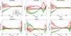 |
Fig. B.1. Mass-matched null bootstrap test. Each panel here corresponds to the second vertical panel of each column in Figs. 2 and 3. The control samples matched in M200m (hatched regions for the (16 − 84)% percentiles, dashed lines for the medians) show the expected distributions under the null hypothesis of no Γ200m dependence. The solid lines, along with the shaded regions, reproduce the original results (red: low-Γ200m; green: high-Γ200m). The separation of the solid lines beyond the hatched regions proves that the observed effects cannot be explained solely by the mass distribution of the low- and high-Γ200m subsamples. |
Thus, our results will be able to confirm a genuine signal of the selection of clusters based on recent accretion, if the actual segregation of the profiles (solid lines and regions) is not compatible with the effect of mass selection (hatched regions and dashed lines).
The effect of the different mass composition of the two subsamples on the profiles is, in all cases, of very limited significance. Regarding the gas density profiles, the only noticeable trend – which, however, falls within the sample variance, i.e. it is not significant – is an increase in the central gas density for the null sample matched to the high-Γ200m distribution. This is the contrary trend to what we have found to occur for the actual samples. A similar effect occurs for the Υ(r), K(r) and P(r) profiles, implying that the patterns that we have reported in the main text cannot be attributed to the mass composition of the samples.
At intermediate radii, the mass-matched control samples have virtually identical profiles for all the studied quantities, which is to be expected since in these regions the profiles are the most self-similar.
Finally, in the cluster outskirts, there is a small effect of the mass selection of the null subsamples on the DM density, temperature, entropy and pressure profiles that matches what we observed in the actual subsamples; specifically, we see an increase in these quantities, approximately at the locations of the splashback and the shock radii, for the null sample matched to the low-Γ200m mass distribution. Again, these differences are not significant given their confidence intervals. In contrast, in all four cases, the actual magnitude of the effect of selecting by Γ200m overshoots the signal that could be solely attributed to mass, and these actual effects are statistically significant. Thus, while a small part of the signal could be attributed to the mass composition, the test shows that, also in this case, our results in the main text reflect the dynamical effect of recent accretion, rather than just a selection bias.
Appendix C: Geometric effects of centre offset and ellipticity on the density and entropy median profiles
In Sects. 3.2 and 3.3, we studied the effects of gas accretion over the last dynamical time on the density and entropy profiles, among others. Subsequently, in Sect. 3.4 we explored the effect of selecting clusters based on several assembly state indicators on entropy and pressure profiles. Among these indicators, some of them contain geometric information about the ICM (i.e. the ellipticity ϵ; or the centre offset Δr). It is thus interesting to explore to what extent the effects that we find are explicitly caused by geometry (i.e. we are computing a radial profile of a system that progressively loses its spherical symmetry) or if there is an actual dynamical effect.
To do so, we realised a spherically symmetric gNFW density profile with inner slope α = 0.5, concentration cvir = 3, and total mass Mvir = 4 × 10¹⁴ M⊙; and an entropy profile following Eq. (D.3) with K0 = 40 keV cm2, K0.1 = 50 keV cm2 and α = 1.1. The entropy profile is then interrupted at ∼2.5Rvir with a sigmoid function to mock the accretion shock. Subsequently, we computed radial profiles following the methodology described in Sect. 2.2, by considering the following geometric transformations:
-
A centre shift, Δr, realised by computing the profiles using as the centre a position displaced by ΔrRvir from the mock centre (density peak).
-
An ellipticity, ϵ, achieved by rescaling the x and z coordinates as
 ,
,  before evaluating the value of the radial profile at each point.
This set-up allows us to study the purely geometric effect of ellipticity and an offset in the centre of the cluster on the density and entropy profiles, which we show, respectively, in the left and right panels of Fig. C.1. The upper panels present the recovered profiles, with colour hue indicating ϵ and lightness encoding Δr. To better highlight the effects, the second panel in each column presents the quotient between these profiles and the input one (i.e. the solid red line in the upper panels).
Regarding density profiles, with Δr = 0 (solid lines), the effect of ellipticity on the median profiles is to reduce densities, especially in the outskirts. However, for realistic ICM ellipticity values (ϵ ≪ 0.5), this effect is contained (≲10%). Centre offset does play a crucial role in altering the recovered, spherical density profiles, as higher Δr considerably lowers central densities. In the lower-left panel we graphically summarise the minimum value of ρ/ρinput and the miscentring radius, rmiscentring, which we define as the innermost point where the input and recovered density profiles start to diverge. This radius is typically in the range rmiscentring ∈ [1, 2]ΔrRvir, and is higher for larger ellipticities.
For the entropy profiles, we observe a central entropy increase when Δr ≠ 0. This result is again stronger for larger ellipticities, as a given radial shell will contain more material from outer elliptical shells. The magnitude of this central entropy boost can reach ≲4 for realistic ICM ellipticities and offsets. Additionally, only for very high ellipticities, a tendency for the entropy peak to displace to slightly inner radii, and to decrease its magnitude (by ∼20% at the unrealistically high ellipticities of ϵ ∼ 0.8). Overall, comparing with the effects seen in Fig. 4 in the main text, this geometrical effects are too weak and the trends we detect cannot be solely explained by geometry.
These geometric effects on the ICM profiles computed assuming spherical symmetry have an effect on the estimation of certain parameters derived from the profiles. Although we rule out the possibility that the trends we observe in our simulation are solely due to geometry, we include this study here for completeness. Fig. C.2 shows how the scale radius (first panel) and the three slope parameters (subsequent panels) of the gNFW depend on ellipticity (horizontal axis) and centre offset (colour) in the mock test. Somewhat surprisingly, the test shows a non-trivial (non-monotonic) relation between mock centre offset and rs (and, thus, NFW concentration). This is a consequence of the high correlation between rs and α (second panel). As soon as we slightly increase Δr, the fit captures an inner slope α ≈ 0, which in turn alters the interpretation of the scale radius (as it no longer corresponds to the position at which the logarithmic slope is −2). Finally, the transition slope (fourth panel), γ, is strongly affected by both miscentring and ellipticity, which contribute to increasing anisotropy within the radial shells considered for computing the profiles and, therefore, smear out the transition.
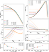 |
Fig. C.1. Density (left) and entropy (right) profiles in the mock test to assess the geometric effects of ellipticity and centre offset. Top row: Profiles, colour-coded by the mock ellipticity value, the line style indicating Δr. Second row: Quotients between the input density and entropy profiles, and the profiles recovered after the geometric transformations. Bottom: Effects of ellipticity and centre offset on flattening the density profiles, increasing the core entropy, and displacing the entropy peak in the outskirts. Here, Δr is represented by the marker shape. |
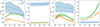 |
Fig. C.2. Effects of ellipticity (horizontal axis within each panel) and centre offset (line colours) on parameter estimations of a gNFW profile. Left to right: Scale radius in units of the virial radius, rs/Rvir; the inner slope, α; the outer slope, β; and the transition sharpness parameter, γ. |
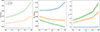 |
Fig. C.3. Effects of ellipticity (horizontal axis within each panel) and centre offset (line colours) on parameter estimations of a Cavagnolo et al. (2009) entropy profile. Left to right: Core entropy excess, K0; power-law normalisation at 0.1R200m, K0.1; and power-law index, α. |
We perform a similar analysis for the entropy profiles in Fig. C.3. In this case, the trends are even cleaner, and suggest that ellipticity alone cannot alter the values of K0 (left-hand side panel), but it can have a significant effect, boosting it by a factor of a few, in the presence of a non-null centre offset. Likewise, the slope of the power-law regime (α) is significantly increased with ellipticity, for the non-null Δr case.
Appendix D: Fitting details
The fits in Sect. 3.6 are carried out using an ensemble MCMC approach, implemented within the emcee package (Foreman-Mackey et al. 2013). In particular, for each fit we initialised 100 chains that were left to explore the posterior space for 2000 steps after an initial burn-in phase of 500 steps. The fits were performed assuming a chi-squared likelihood function in the logarithm of the target variable (e.g. log10ρ, log10K), where only the errors in the dependent variable are taken into account. Priors are flat within the bounds specified below for each case.
Fits for the NFW concentration. The model function is
 (D.1)
(D.1)
where we adopt flat priors on log10(ρ0/ρB)∈[0, 8] and rs/Rvir ∈ [0.01, 1]. The fits were restricted to the radial range where ρ/ρB > 1.
Fits to the gNFW functional form. For the generalised NFW profile, we consider the functional form
![Mathematical equation: $$ \begin{aligned} \rho (r) = \frac{\rho _0 \, \cdot \, 2^\frac{\beta -\alpha }{\gamma }}{\left(\frac{r}{r_s}\right)^{\alpha } \left[1 + \left(\frac{r}{r_s}\right)^\gamma \right]^\frac{\beta -\alpha }{\gamma }}, \end{aligned} $$](/articles/aa/full_html/2026/02/aa57496-25/aa57496-25-eq25.gif) (D.2)
(D.2)
where the power of two term is added to remove the covariance of ρ0 with the slope parameters (so that ρ0 explicitly represents the normalisation of the profile at rs). While the density and radius normalisation parameters keep the same priors, for the slopes we consider the bounds α, β ∈ [0, 10], γ ∈ [0.2, 5]. The fits were restricted to the radial range where ρ/ρB > 1 (P/P200m > 1 for the pressure profiles).
Fits to the entropy profile. For the entropy profile, we adopted the functional form by Donahue et al. (2006) and Cavagnolo et al. (2009), modified to normalise the power law at 0.1R200m instead of a constant 100 kpc,
 (D.3)
(D.3)
where, in this case, the priors are flat in K0/K200m ∈ [0, 1], K0.1/K200m ∈ [0, 10], and α ∈ [0, 5]. To make the results representative of the typical self-similar range of entropy profiles (see lower panel of Fig. 6), and mitigate the effects of over-cooling in the centre and the accretion shocks in the outskirts, the likelihood function is computed only over the radial range 0.1 ≤ r/R200m ≤ 2.
Polynomial fits. The fits for summarising the trends of the profile fit parameters with accretion rate are not performed by MCMC sampling, but instead we just proceed with an ordinary least-squares fit. The process for deciding the degree of the fitting polynomial is analogous to the one described in Vallés-Pérez et al. (2023). However, here we also account for the errors in the independent variable, by estimating the local slope of the fitting function at each point and iterating the process. This is crucial in this case, since the width of the bins in Γ200m is highly variable.
All Tables
Summary statistics accounting for the mass distribution of our group and cluster sample.
All Figures
|
Fig. 1. Comparison between mean (solid red line), median (solid cyan line), and mode (dashed orange line) gas density profiles in two galaxy clusters (corresponding to the two panels). In addition to the standard mean profiles, mean profiles with masked substructures are shown by the dashed red lines. Light-grey lines indicate the individual directional profiles, while dotted cyan lines represent the (16−84)% percentiles at each r to give a better idea of the width of the density distribution. Dotted dark-blue lines indicate the thresholds for the substructure cleaning algorithm from which the dashed red line is obtained. The insets provide a zoomed-in view of two regions to highlight the differences among the profiles. The blue-filled line at the right of the right-hand panel inset depicts the density distribution at r ∼ 3Rvir, highlighting its bimodality. |
| In the text | |
|
Fig. 2. Mass distribution for the highest accreting third (green) and lowest accreting third (red) of the sample. Left: Gas density. Center: DM density. Right: Baryon depletion. Top row: Profiles stacked over each subsample, together with the whole population (grey lines). Second row: Each class normalised by the ensemble average. Third row: Logarithmic slopes of the profiles, together with an indication of the radius of minimum slope. Bottom row: Correlation between the profiles and accretion rate Γ200m controlling for M200m. |
| In the text | |
|
Fig. 3. Thermodynamic state of the highest-Γ200m third (green) and the lowest-Γ200m third (red) of the sample. Left: Temperature. Middle: Entropy. Right: Thermal pressure. The vertical panels within each column contain the same information as in Fig. 2. |
| In the text | |
|
Fig. 4. Effect of individual indicators of assembly state on entropy profiles. Top: Spearman (partial) correlation coefficients of each indicator and profile values at each r/R200m. Higher magnitudes (either positive or negative) indicate a greater influence of the value of the indicator on the profile value at this particular radius. Middle: Effect of selecting clusters based on each parameter on the location and depth of the steepest logarithmic slope of the entropy profile. The crosses correspond to the profile stacked over the one-third most relaxed subsample (according to the given indicator), while the filled dots correspond to the most disturbed third. Bottom panel: Similar to the middle panel, but with the location and height of the entropy peak. The blue regions in the middle and bottom panels indicate the 68% confidence region for the determination of the corresponding locations over each of the Δr-based subsamples (as an example), obtained by bootstrap resampling. |
| In the text | |
|
Fig. 5. Effect of individual indicators of assembly state on the pressure profiles. Top: Similar to that in Fig. 4, but with the pressure profiles. Bottom: Similar to the middle panel in Fig. 4, but with the pressure profiles. The colour code and other figure elements are kept the same as in the aforementioned figure. |
| In the text | |
|
Fig. 6. Deviations from sphericity and self-similarity of cluster profiles. Top: ICM asphericity, 𝒜(r), profiles for different quantities. Middle: Spearman rank correlation of profile asphericity with accretion rates. Bottom: Departure from self-similarity, 𝒮(x), of the profiles. The dashed lines correspond to the quotient of this quantity among the highest- and lowest-accreting thirds of the sample. |
| In the text | |
|
Fig. 7. Concentration c200m = R200m/rs (with rs being the best-fit scale radius of the NFW functional form) of the DM (red), and gas (blue) profiles stacked in deciles of accretion rate Γ200m over the last dynamical time. The dots indicate the results for each decile of accretion rate, with 1σ error bars, while the lines show linear fits with their confidence regions. |
| In the text | |
|
Fig. 8. Dependence of the inner slope (α, left), the outer slope (β, middle), and the transition parameter (γ, right) of a gNFW model on the accretion rate, for the DM density (red), gas density (blue), and pressure (green) profiles. Dots with error bars represent the results from the fit to the profiles stacked over each decile in Γ200m. The lines represent least-squares polynomial fits, with the dark-shaded regions showing the fit uncertainty, and the light-shaded regions also including the uncertainty of the dots added in quadrature (assuming it depends linearly on Γ200m). |
| In the text | |
|
Fig. 9. Variation of the core excess entropy (K0, red line in the upper panel), power-law normalisation (K0.1, blue line in the upper panel) and power-law index (lower panel) with accretion rate. All plot elements are equivalent to those in Fig. 8. |
| In the text | |
|
Fig. B.1. Mass-matched null bootstrap test. Each panel here corresponds to the second vertical panel of each column in Figs. 2 and 3. The control samples matched in M200m (hatched regions for the (16 − 84)% percentiles, dashed lines for the medians) show the expected distributions under the null hypothesis of no Γ200m dependence. The solid lines, along with the shaded regions, reproduce the original results (red: low-Γ200m; green: high-Γ200m). The separation of the solid lines beyond the hatched regions proves that the observed effects cannot be explained solely by the mass distribution of the low- and high-Γ200m subsamples. |
| In the text | |
|
Fig. C.1. Density (left) and entropy (right) profiles in the mock test to assess the geometric effects of ellipticity and centre offset. Top row: Profiles, colour-coded by the mock ellipticity value, the line style indicating Δr. Second row: Quotients between the input density and entropy profiles, and the profiles recovered after the geometric transformations. Bottom: Effects of ellipticity and centre offset on flattening the density profiles, increasing the core entropy, and displacing the entropy peak in the outskirts. Here, Δr is represented by the marker shape. |
| In the text | |
|
Fig. C.2. Effects of ellipticity (horizontal axis within each panel) and centre offset (line colours) on parameter estimations of a gNFW profile. Left to right: Scale radius in units of the virial radius, rs/Rvir; the inner slope, α; the outer slope, β; and the transition sharpness parameter, γ. |
| In the text | |
|
Fig. C.3. Effects of ellipticity (horizontal axis within each panel) and centre offset (line colours) on parameter estimations of a Cavagnolo et al. (2009) entropy profile. Left to right: Core entropy excess, K0; power-law normalisation at 0.1R200m, K0.1; and power-law index, α. |
| In the text | |
Current usage metrics show cumulative count of Article Views (full-text article views including HTML views, PDF and ePub downloads, according to the available data) and Abstracts Views on Vision4Press platform.
Data correspond to usage on the plateform after 2015. The current usage metrics is available 48-96 hours after online publication and is updated daily on week days.
Initial download of the metrics may take a while.