© The Authors 2026

1. Introduction

Observations of CO at high redshift with interferometric facilities have advanced our understanding of the cosmic evolution of cool gas and its role in driving the star formation rate density (SFRD, Madau & Dickinson 2014; Péroux & Howk 2020; Walter et al. 2020). Star formation occurs in cold, dense molecular clouds mainly composed of H₂, which cannot be directly observed at low temperatures. As the second most abundant molecule and a key coolant of the cold ISM, CO is widely used as a tracer of cold molecular gas (McKee & Ostriker 2007; Carilli & Walter 2013).

Carbon monoxide emits a ladder of rotational transitions with energies determined by the quantum number J_up. At high redshift, the ground-state transition CO(1–0) – a key tracer of cold molecular gas – is often not detected, because the signal is very faint and its rest-frame frequency shifts outside the well-covered observational bands. Consequently, higher-J_up lines (≥2) are typically used instead. These must be corrected by an excitation factor before applying the standard CO-to-H₂ conversion (α_CO). The resulting excitation pattern is the CO spectral-line energy distribution (SLED). Other tracers of the cold ISM include dust continuum (e.g., Scoville et al. 2017; Magnelli et al. 2020) and atomic lines such as [CI] (e.g., Valentino et al. 2018; Gururajan et al. 2023). In the last ten years, deep CO surveys with NOEMA (Boogaard et al. 2020, 2023), ALMA (ASPECS, Decarli et al. 2020), and the JVLA (COLDz, Riechers et al. 2019) have measured the molecular gas density, ρ_H2, up to z ∼ 5. These studies reveal an increase by a factor of ∼7 in ρ_H2 from z = 0 to z ∼ 1–3, aligning with the peak of the SFRD (Walter et al. 2020), and followed by a decline at higher redshift.

Despite uncertainties in the CO-to-H₂ conversion factor (Bolatto et al. 2013), galaxies on the main sequence at z ∼ 1–3 show higher molecular gas fractions than local ones (Tacconi et al. 2013, 2018, 2020; Saintonge et al. 2013; Genzel et al. 2015), suggesting that elevated star formation during cosmic noon is driven by a higher gas fraction available in galaxies to form stars.

The shape of the CO SLED reflects molecular gas conditions: low-J lines trace diffuse gas (∼10³ cm⁻³; e.g., Harris et al. 2010; Ivison et al. 2011; Riechers et al. 2011), while mid-J lines (J_up = 5–7) trace denser, star-forming regions (∼10⁵ cm⁻³ e.g., Daddi et al. 2015; Lu et al. 2017). Additional processes such as feedback, shocks, turbulence, active galactic nuclei (AGN) and X-ray heating also affect the SLED. Thus, the SLED provides key insights into the physical conditions of the ISM in galaxies. Measured SLEDs can be compared to those of local main-sequence galaxies; starbursts (Greve et al. 2014; Rosenberg et al. 2015; Lu et al. 2017); high-redshift, dusty star-forming galaxies (Danielson et al. 2011); and quasars (e.g., Weiß et al. 2007; Bradford et al. 2009; Li et al. 2020; Kade et al. 2024). However, the significant variation between individual objects at high redshift makes SLEDs challenging to interpret.

Line-intensity mapping (LIM) is a powerful complement to the high-redshift CO observations to obtain a cosmic view of the global CO-emitting properties of galaxies (see the reviews of Kovetz et al. 2017 and Bernal & Kovetz 2022). LIM consists of an accurate mapping of the fluctuations of the CO background intensity produced by the whole galaxy population as a function of sky coordinates and redshift. This observational technique is thus sensitive to CO emitters fainter than the detection limits of galaxy surveys, and thus probes both the clustering of CO emitters and ρ_H2(z), free of any source selection bias.

Among the various LIM experiments, those operating in the millimeter domain include the South Pole Telescope Summertime Line Intensity Mapper (SPT-SLIM Karkare et al. 2022, J_up ≥ 2) and the CarbON CII line in post-rEionization and ReionizaTiOn epoch (CONCERTO; CONCERTO Collaboration 2020, J_up ≥ 2) both targeting J_up ≥ 2. Other current and forthcoming experiments are conducted in submillimeter wavelengths (primarily targeting the [C_II] line), such as the Fred Young Submillimeter Telescope (FYST)/CCAT-prime with its instrument Prime-Cam (CCAT-Prime Collaboration 2023, J_up ≥ 2), the Tomographic Ionized Carbon Intensity Mapping Experiment (TIME; Crites et al. 2014; Sun et al. 2021, J_up ≥ 2), and the EXperiment for Cryogenic Large-Aperture Intensity Mapping (EXCLAIM, Essinger-Hileman et al. 2020, J_up ≥ 4). These experiments have access to the upper transitions in the CO SLED originating from different redshifts.

The (sub)millimeter LIM experiments will complement the direct constraints on ρ_H2(z) obtained from radio-LIM experiments that primarily target the CO(1–0) transition, such as COMAP (Cleary et al. 2022), and will help refine the relation between CO(1–0) emission and the molecular gas mass (e.g., Silva et al. 2021). Fluctuations mapped by LIM are typically analyzed using the auto-power spectrum. However, the auto-power spectrum is contaminated by the signal from continuum emission and line interlopers, i.e., other lines from other sources redshifted in the same frequency range.

On the one hand, one can analyze the total signal formed by the sum of the contribution of the different CO lines from different redshifts with a model. This was carried out by the mmIME experiment (Keating et al. 2020), which provided the first constraints on total CO shot noise using ALMA and ACT archival data, and derived constraints on the CO(2–1), CO(3–2), and CO(4–3) auto powers at z = 1.3, z = 2.5, and z = 3.6, respectively. Béthermin et al. (2022) also compared their empirical CO model to the total CO power constraints of Keating et al. (2020), showing agreement with the mmIME measurements.

On the other hand, one can use component-separation methods to obtain information on individual lines directly. In this work, we demonstrate that the cross-correlation between LIM and galaxy surveys can be used to extract the signal from individual CO lines. Cross-correlation between two large-scale structure (LSS) tracers, either between two LIM surveys (e.g., Beane et al. 2019, Murmu et al. 2021, Schaan & White 2021, Padmanabhan et al. 2022, Chung 2023, and Roy & Battaglia 2024 for various lines) or with external galaxy surveys (e.g., Wolz et al. 2017, Chung et al. 2019, and Visbal & McQuinn 2023), allows one to isolate the emission originating from the same cosmic volume and to mitigate contamination from interlopers. Indeed, the uncorrelated interloper signal does not contribute on average, but instead acts as an additional source of noise.

Assuming that continuum contamination from the cosmic infrared background has been removed beforehand (e.g., Yue et al. 2015 and Van Cuyck et al. 2023), we investigated how the CO background SLED and ρ_H2(z) can be constrained from the J ≥ 1 CO transitions up to z = 3.0 using the cross-correlation between LIM data and spectroscopic galaxy surveys.

This paper is organized as follows. In Sect. 2, we present the fiducial SIDES model on which our study is based. In Sect. 3, we detail the cross-power spectrum formalism used in this paper. Then, in Sect. 4, we present and discuss our results on the reconstruction of the CO background SLED and the cold-gas cosmic density, ρ_H2. We assess the feasibility of measuring the cross-power with a CONCERTO-like experiment in Sect. 5. Finally, we summarize our conclusions and outline future directions in Sect. 6.

2. SIDES

Several models of CO line intensity mapping exist in the literature (e.g., Sun et al. 2021; Breysse et al. 2022; Yang et al. 2022; Karoumpis et al. 2024). Here, we used the simulated infrared dusty extragalactic sky (SIDES) described in Béthermin et al. (2017, 2022) and Gkogkou et al. (2023), which offers a realistic and observationally motivated framework. SIDES uses a dark-matter halo catalog derived from the 117 deg² light cone of the Uchuu N-body simulation as input (Ishiyama et al. 2021), achieving the highest mass resolution for a field of this size. SIDES incorporates extensive knowledge of dusty galaxies and the cosmic infrared background (CIB) to reproduce statistical properties across mid-infrared to millimeter wavelengths, including galaxy redshift distributions, number counts, continuum- and line-luminosity functions, CIB fluctuations, SFRD, and the shot-noise level of CO at 3 mm (Keating et al. 2020). The SIDES-Uchuu simulation thus provides an optimal compromise between large-field coverage and detailed astrophysical modeling. SIDES adopts the cosmology of the Planck Collaboration XIII (2016) and a Chabrier (2003) initial mass function (IMF).

2.1. Galaxy population synthesis

The simulated infrared dusty extragalactic sky establishes a relation between stellar mass and halo mass via abundance matching, generating a galaxy light cone complete down to 10⁷ M_⊙ up to z = 7 (Gkogkou et al. 2023). A scatter of 0.2 dex is applied to the halo mass–stellar mass relation resulting from the abundance-matching procedure. Similarly, the other observational relations used to derive a galaxy’s physical parameters incorporate an appropriate scatter.

The SIDES framework uses a model with two star-formation modes. Galaxies are first classified as star-forming or passive following the observed fraction of star-forming galaxies as a function of mass and redshift from Davidzon et al. (2017). Passive galaxies, which are faint in the far-infrared and millimeter wavelengths (e.g., Whitaker et al. 2021), are excluded from further modeling. Star-forming galaxies are assigned to the redshift-evolving main sequence (MS) or to starburst (SB) categories, according to the redshift-dependent fraction described in Béthermin et al. (2012), and their SFR is drawn accordingly, with a 0.3 dex scatter. The SFRs are used to compute infrared luminosities (L_IR) via the Kennicutt (1998) relation, which are then used in the line-flux calculation.

2.2. CO lines

The luminosity of the CO(1–0) transition is computed using the L_IR − L_{CO(1 − 0)} relation from Sargent et al. (2014), with a scatter of 0.2 dex. For SB galaxies, which deviate from this relation, an empirical offset of −0.46 dex is applied. SIDES models the SLED of MS galaxies up to J = 8 using a combination of clumpy and diffuse gas, with each component adopting a SLED from Bournaud et al. (2015). The relative contributions of the clumpy and diffuse gas are set so that the CO(5–4)/CO(2–1) ratios follow the relation of Daddi et al. (2015), with the mean radiation field parameter ⟨U⟩. In the SIDES framework, ⟨U⟩ is used to assign the dust SED and follows a simple redshift evolution that includes a 0.2 dex scatter:

$$\begin{array}{c}\hfill {log}_{10}\left[{⟨U⟩}_{\mathrm{MS}}(z)\right]={log}_{10}\left[{⟨U⟩}_{\mathrm{MS}}(z=0)\right]+{\alpha }_{⟨U⟩}\times z,\end{array}$$(1)

where ⟨U⟩_MS(z = 0) and α_⟨U⟩ are constant. As a result, the scatter in ⟨U⟩ causes MS galaxies to exhibit a variety of SLEDs, which generally become more excited with redshift. SB galaxies, in contrast, follow the SLED templates from Birkin et al. (2021).

2.3. Other CO-interloping lines

The luminosity of the two fine-structure lines [C_I] are derived from empirical relations between luminosity ratios, which were calibrated using the observations from Valentino et al. (2020). The calibration of these relations are presented in Béthermin et al. (2022).

First, Valentino et al. (2020) find that the [CI](1–0)/CO(4–3) is consistent across the different populations of galaxies and redshifts studied. Observations show that the [CI](1–0)/L_IR and CO(4–3)/L_IR ratios correlate with a dispersion of 0.2 dex. This relation is therefore used to derive [CI](1–0).

The [CI](2–1)/[CI](1–0) ratio traces the excitation temperature. This excitation also influences the CO SLED, making the CO(7–6)/CO(3–4) ratio a good proxy for the excitation temperature in SIDES. These two ratios correlate with a scatter of 0.19 dex, and they are used to derive the [CI](2–1) line luminosity.

Finally, [CII] is an important interloper, especially for frequency ν > 270 GHz (z_[CII] ≤ 6). We adopted the [CII] luminosity from the L_[CII]-SFR empirical relation calibrated in the local Universe (De Looze et al. 2014) as our fiducial [C_II] luminosity.

2.4. Spectral cubes

From the generated galaxy catalog, mock LIM spectral cubes are produced in sky coordinates for cross-correlation with spectroscopic galaxy surveys. Cross-correlating LIM maps with redshift catalogs isolates emission from the same cosmic volume and mitigates contamination from interloping lines, which contribute additional noise rather than a systematic bias.

The field-to-field variance of the power spectrum impacts millimeter-LIM surveys over small areas, though this effect decreases for larger survey fields (Keenan et al. 2020; Gkogkou et al. 2023). We therefore extracted 12 light cones of 9 deg² from the 117 deg² SIDES-Uchuu simulation to minimize the impact of cosmic variance.

2.4.1. Sky-coordinate-redshift CO cubes

For each 9 deg² field, intensity maps spanning δz = 0.05 are generated from z = 0.5 to 3.0 for CO transitions with J_up = 1–8. Table 1 lists the observed frequency of each CO line and redshift z. The resulting spectral resolutions δν are given by δν = δz × (1 + z) ν_obs and are also provided in Table 1, aligning well with the spectral resolution of CONCERTO.

In the intensity maps, intensities from all sources up to 10⁷ M_⊙ are included because the LIM surveys do not suffer from any selection effect. The emission of interlopers is added to produce interloper-contaminated maps.

2.4.2. Galaxy number-density-contrast cubes

To measure the cross-correlation between the CO and galaxies, number density-contrast cubes are generated for each light cone and redshift, spanning the same δz as the CO cubes. The depth of the survey used to generate galaxy maps directly impacts the significance of cross-power spectrum detection (e.g., Chung et al. 2019). Laigle et al. (2016, hereafter L16) demonstrated that a limiting magnitude of k_s,lim ≤ 24.0 ensures 90% completeness for galaxies with $M_{\ast ,\lim }^{\mathrm{L}16}\sim {10}^{10}{\mathrm{M}}_{\odot }$ at z = 2−3 in the COSMOS2015 catalog. Consequently, we include galaxies down to 10¹⁰ M_⊙ and up to z = 3 in our galaxy cubes.

We aim to compute the power spectrum of the galaxy numbe density contrast, δρ/ρ₀, where ρ₀ is the mean number density. Thus, each galaxy number-density map is normalized by its mean density to produce galaxy number-density contrast maps.

Assuming that the cross-power spectrum remains constant over Δ z = 0.25, we computed the power spectrum by averaging five spectral channel maps with Δ z = 0.05. Figure 1 shows the number of galaxies used for cross-correlation, averaged over the 12 light cones in Δ z = 0.25 as a function of redshift. The right axis of Fig. 1 shows the corresponding shot noise of the contrast density.

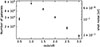Fig. 1. Right axis: Mean number of galaxies per galaxy cube covering 9-deg2 and Δz = 0.25, as a function of redshift. The error bars come from the dispersion over the twelve independent light cones. Left axis: The associated shot noise of galaxy’s number density contrast in the 9-deg2 fields.

The (cross-) power spectra derived from the mock cubes are called the simulation-based (cross-) power spectra. Figure 2 shows the CO(4–3) and corresponding galaxy maps, obtained by averaging five maps of δz = 0.05 along the redshift axis (and thus Δz = 0.25) for one of 9 deg² light cones.

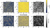Fig. 2. From left to right: Images of SIDES intrinsic CO(4–3) cube integrated along spectral axis over Δz = 0.25, the same CO(4–3) cube including contamination from line interlopers, and the galaxy cube integrated over the same redshift range. The top row corresponds to z = 0.5 and the bottom row to z = 3.0. Continuum contamination is assumed to have been removed beforehand.

2.5. Relevant scales

In this work, we took advantage of the linearity of large scales, where the power spectrum is dominated by the two-halo term of galaxy clustering. To ensure a more robust modeling framework and mitigate the impact of nonlinearities and small-scale systematics, we restricted our modeling and analysis – detailed in the following section – to scales of k ≤ 0.35 Mpc⁻¹. On these scales, the shot noise contribution (strongly dependent on astrophysical details) is subdominant, and instrumental beam smearing has a negligible impact. While the one-halo term could, in principle, contribute, we show later that its impact is negligible on the considered scales (k ≤ 0.35 Mpc⁻¹).

This choice of scale also constrains the acceptable redshift uncertainty, expressed as dz/(1 + z), that an ancillary survey must achieve in order to avoid attenuating the cross-power on the relevant scales. Following the formalism of Chung et al. (2019, Appendix B), we find that the typical redshift uncertainty of COSMOS2015, which is dz/(1 + z) = 3 × 10⁻², leads to an attenuation of the cross-power spectrum by a factor of ≤0.1 at k = 0.35 Mpc⁻¹. By contrast, a redshift uncertainty of dz/(1 + z) = 1 × 10⁻³, representative of spectroscopic surveys, results in a ≤10% attenuation (a factor of ≥0.9) at z ≥ 1, which is smaller than the interloper-induced systematics, as we will see in Sect. 4. Increasing to dz/(1 + z) = 3 × 10⁻³ increases the attenuation to 0.5 at z = 1 and to 0.85 at z = 3.0. Although current COSMOS2015 and COSMOS2020 do not reach this redshift accuracy, COSMOS is part of the Euclid Wide Survey, which will provide spectroscopic redshifts down to 22.5–23 in AB magnitudes for the bulk of the known COSMOS sources. Therefore, assuming a future spectroscopic survey, we disregarded redshift errors in our galaxy maps for the considered scales: k ≤ 0.35 Mpc⁻¹.

3. Power spectrum model

In this section, we describe the model that we used to interpret the simulation-based angular cross-power spectra measured from the mock cubes described.

3.1. Mean background brightness

The mean background brightness, B_ν, at a given observed frequency, ν, produced by point sources is

$$\begin{array}{c}\hfill B_{\nu }[\mathrm{Jy}/\mathrm{sr}]={\displaystyle \int {\mathrm{S}}_{\nu }^2}\frac{\mathrm{dN}}{\mathrm{dS}}\mathrm{d}ln{\mathrm{S}}_{\nu },\end{array}$$(2)

where $\frac{\mathrm{dN}}{\mathrm{dS}}$ are the differential number counts per solid angle, and dS_ν is the observed flux-density interval. The relation between the observed flux density integrated along the line velocity profile I_ν and the spectral luminosity L_{(1 + z)ν} (in L_⊙) for a source at a luminosity distance D_L in Mpc observed at ν in GHz is (Carilli & Walter 2013)

$$\begin{array}{c}\hfill I_{\nu }[\mathrm{J}y.km.s^{-1}]=\frac{1}{1.04\times {10}^{-3}{D}_L^2(z)\nu }\times L_{(1+z)\nu }.\end{array}$$(3)

The line flux density, S_ν, of the source in a frequency channel measuring δν in width is then

$$\begin{array}{c}\hfill S_{\nu }[\mathrm{Jy}]=\frac{{\nu }_{\mathrm{obs}}}{c\times \delta \nu }\times I_{\nu },\end{array}$$(4)

with the speed of light, c, given in kilometers per second.

3.2. Cross-power spectrum

The clustering of galaxies introduces correlations in the anisotropies. This gives rise to a clustering term in the cross-power spectrum, which encodes the clustered distribution of the line emitters. At large scales, it can be modeled using a simple linear bias model of the following form:

$$\begin{array}{c}\hfill P_{{\mathrm{J}}_{\mathrm{up}}-\mathrm{gal}}^{\mathrm{clust}}(k_{\theta },z)=B_{\nu }^{{\mathrm{J}}_{\mathrm{up}}}(z)b_{\mathrm{eff}}(z)b_{\mathrm{gal}}(z)\times P_{\mathrm{matter}}^{2\mathrm{D}}(k_{\theta },z),\end{array}$$(5)

where B_ν is given by Eq. (2). The parameters b_eff and b_gal are the linear clustering biases for the line surface brightness and the galaxies, respectively. As we worked with circular-averaged angular power spectra, $P_{\mathrm{matter}}^{2\mathrm{D}}(k_{\theta },z)$ is the 2D, linear, angular power spectrum of matter at the angular wave number k_θ.

The 2D angular power spectrum relates approximately to the 3D spherically averaged power spectrum P^3D(k, z) at the comoving wave number $k=\sqrt{(k_{//}^2+k_{\perp }^2)}$ via (Neben et al. 2017; Yue & Ferrara 2019)

$$\begin{array}{c}\hfill P^{2\mathrm{D}}(k_{\theta },z)=\frac{1}{{\mathrm{D}}_{\mathrm{c}}^2\mathrm{\Delta }{\mathrm{D}}_{\mathrm{c}}}{P}^{3\mathrm{D}}(k=\frac{2\pi k_{\theta }}{{\mathrm{D}}_{\mathrm{c}}},z),\end{array}$$(6)

where D_c is the comoving distance in megaparsecs and ΔD_c is the comoving thickness in the radial direction:

$$\begin{array}{c}\hfill \mathrm{\Delta }{D}_c=\frac{c(1+z)\delta \nu }{H(z)\nu },\end{array}$$(7)

where H(z) is the Hubble parameter at redshift z. This assumes that ΔD_c ≪ D_c and that $P_{\mathrm{matter}}^{3\mathrm{D}}$ does not vary significantly across the frequency channel. The 3D-matter power spectrum, $P_{\mathrm{matter}}^{3\mathrm{D}}(z,k),$ was calculated using CAMB (Howlett et al. 2012).

The linear clustering bias, b_eff, quantifies the clustering amplitude ratio between the line surface brightness and the underlying dark-matter distribution on linear scales:

$$\begin{array}{c}\hfill b_{\mathrm{eff}}(z)=\frac{\int dMn(M,z)b_h(M,z)L(M,z)}{\int dMn(M,z)L(M,z)},\end{array}$$(8)

where n(M,z) is the emitting galaxy’s number density and L(M,z) their luminosity given by the SIDES model. The term b_h is the bias of the halo in which a galaxy lives with respect to the underlying dark-matter distribution. Since all the galaxies in the same redshift range have similar luminosity distance, b_eff can be re-expressed in terms of flux density:

$$\begin{array}{c}\hfill b_{\mathrm{eff}}(z)=\frac{\int dMn(M,z)b_h(M,z)S_{\nu }(M,z)}{\int dMn(M,z)S_{\nu }(M,z)}·\end{array}$$(9)

Similarly, the clustering bias for the galaxies, b_gal, is given by

$$\begin{array}{c}\hfill b_{\mathrm{gal}}(z)=\frac{\int dM{n}_{\mathrm{gal}}(M,z)b_h(M,z)}{\int dM{n}_{\mathrm{gal}}(M,z)},\end{array}$$(10)

where n_gal(M,z) is the galaxy’s number density.

We ignore the shot noise and one-halo term in our analysis, as it is negligible at the large scales studied here (i.e., below k < 0.35 Mpc⁻¹). The one-halo term primarily dominates on smaller, nonlinear scales, corresponding to the clustering of galaxies within the same dark-matter halo, and its contribution diminishes significantly on larger scales where the two-halo term, representing correlations between halos, becomes dominant. This assumption is supported in the context of CIB analysis, where the one-halo term is reported to be subdominant on these scales (e.g., Viero et al. 2013).

3.3. Auto-power spectra

The clustering in the auto-power spectrum of the line emitters is

$$\begin{array}{c}\hfill P_{{\mathrm{J}}_{\mathrm{up}}}^{\mathrm{clust}}(k_{\theta },z)=B_{\nu }^2(z)b_{\mathrm{eff}}^2(z)P_{\mathrm{matter}}^{2\mathrm{D}}(k_{\theta },z),\end{array}$$(11)

and the line auto-shot power is given by

$$\begin{array}{c}\hfill P^{\mathrm{shot}}(z)={\displaystyle \int S_{\nu }^3}\frac{\mathit{dN}}{\mathit{dS}}dln{S}_{\nu }.\end{array}$$(12)

Similarly, the clustering in the galaxy’s auto-power spectrum is modeled as

$$\begin{array}{c}\hfill P_{\mathrm{gal}}^{\mathrm{clust}}(k_{\theta },z)=b_{\mathrm{gal}}^2(z)P_{\mathrm{matter}}^{2\mathrm{D}}(k_{\theta },z),\end{array}$$(13)

and the galaxy shot noise is given by

$$\begin{array}{c}\hfill P^{\mathrm{shot}}(z)=\frac{1}{{\overline{n}}_{\mathrm{gal}}}·\end{array}$$(14)

3.4. Clustering biases in SIDES-Uchuu

In Eq. (5), the mean intensity, B_ν, of a line background is degenerated with the clustering bias of CO emitters, b_eff, and galaxies, b_gal. In practice, b_gal is measured directly from the galaxy catalog, but b_eff has to be obtained from a model. Because we work with a simulation, we can derive the effective clustering biases b_eff^SIDES and b_gal^SIDES specific to the SIDES-Uchuu simulation from the auto-power spectra.

To obtain SIDES-specific biases (b_eff/gal^SIDES) of each CO line at a redshift of z in a subfield, we measured the simulation-based auto-power spectra, P_J/gal. Using the scales below k < 0.35 Mpc⁻¹, we fit the clustering power, P_J/gal^clust, from Eqs. (11) and (13), with b_eff/gal^SIDES as the free parameter to be found. Figure 3 shows an example of this procedure at z = 0.5 for CO(4–3) in one of the 12 subfields. Even though the one-halo term might introduce a slight bias, we demonstrate later that its impact is negligible at the considered scales (k < 0.35 Mpc⁻¹).

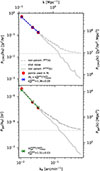Fig. 3. Upper panel: CO(4–3) auto-power spectrum at z = 0.5. The dashed gray line shows the simulation-based auto-power spectrum Ptot(k). It is the average over the five auto-power spectra of CO(4–3) maps, each map spanning δz = 0.05. The dotted gray line shows the average shot noise component. Subtracting the shot noise yields the clustering Pclust(k) shown with the solid gray line. The clustering (Eq. (11)) is fit to Pclust at large scales only, using the red points. From this fit, the effective clustering bias in SIDES, $b_{\mathrm{eff}}^{\mathrm{fit}}$, is estimated. Lower panel: Same procedure for galaxies’ auto-power spectra and $b_{\mathrm{gal}}^{\mathrm{fit}}$, still at z = 0.5.

4. CO-galaxy cross-correlation

In this section, we present the results obtained from the 12 light cones cut in SIDES-Uchuu. For each subfield, we built the spectral cubes at six redshifts from z = 0.5 to 3.0, following the method described in Sect. 2.4, as well as the associated galaxy number density-contrast cubes. We cross-correlated each pair consisting of an interloper-contaminated CO intensity cube and a corresponding galaxy density-contrast cube, and measure the simulation-based angular (i.e, in sky coordinates) cross-power spectrum. The results for each redshift and CO transition are averaged over the 12 subfields and presented below. The dispersion among fields is also used to estimate uncertainties.

In the following, Sect. 4.1 explains the reconstruction of the CO background SLED from the measured cross-power spectra and compares to the intrinsic SIDES CO SLED. Sect. 4.2 focuses on the measurement of bias-weighted intensities, and Sect. 4.3 focuses on the reconstruction of the effective bias. Finally, Sect. 4.4 discusses the estimation of the cosmic cold-gas density, ρ_H2(z), using the results of the two previous sections.

4.1. Spectral line energy distribution

The SLED of the emitter’s background is defined as the background intensity ratio between a transition, J_up, and a reference transition. It can be obtained directly by taking the ratio of two cross-power spectra, to simplify the clustering bias and the matter-power-spectrum factors in Eq. (5):

$$\begin{array}{c}\hfill {\mathrm{R}}_{{\mathrm{J}}_{\mathrm{up},\mathrm{ref}}}^{{\mathrm{J}}_{\mathrm{up}}}(z)=\frac{P_{{\mathrm{J}}_{\mathrm{up}}-\mathrm{gal}}^{\mathrm{clust}}(k_{\theta },z)}{P_{{\mathrm{J}}_{\mathrm{up},\mathrm{ref}}-\mathrm{gal}}^{\mathrm{clust}}(k_{\theta },z)}=\frac{B_{\nu }^{{\mathrm{J}}_{\mathrm{up}}}(z)}{B_{\nu }^{{\mathrm{J}}_{\mathrm{up},\mathrm{ref}}}(z)}⧸\frac{b_{\mathrm{eff}}(z)b_{\mathrm{gal}}(z)\times P_{\mathrm{matter}}^{2\mathrm{D}}}{b_{\mathrm{eff}}(z)b_{\mathrm{gal}}(z)\times P_{\mathrm{matter}}^{2\mathrm{D}}},\end{array}$$(15)

which is only true if b_eff is the same for all CO lines, and we see that it is indeed the case for SIDES in Sect. 4.3.

Its relevance is twofold. First, the CO background SLED itself, and its evolution with redshift, can provide meaningful information on the physical condition of the cold gas in the interstellar medium of galaxies. Second, deriving the excitation from the SLED is essential to estimating the cold-gas density, ρ_H2, from CO transitions with J_up > 1, as the SLED is required to convert the background intensities of these transitions into their equivalent CO(1–0) background intensity.

Without access to the J_up = 1 transition, the millimeter-LIM must first derive the CO SLED and then assume an excitation to connect any level to the J_up = 1 level. In this work, we adopt the CO(3–2) line as the reference, as it allows us to probe up to z = 1.5, whereas CO(2–1) is only observable at z = 0.5 within the CONCERTO bandwidth.

The simulation-based cross-power spectra of all CO lines are measured in each of the 12 simulated light cones at z = 0.5, 1.0, 2.0, 2.5, and 3.0. The ratio of the power spectra between a given CO transition and the CO(3–2) line is then taken at each redshift using the scales below k < 0.35 Mpc⁻¹.

Figure 4 shows with circles the SLED of the CO background obtained from the simulation-based cross-power spectra. We note that the data points have been slightly shifted along the x-axis for clarity. Solid lines and shaded areas represent the mean SLED and its 1σ dispersion over all galaxies in the SIDES catalog. The color-code corresponds to the six redshift intervals, from z = 0.5 to 3.0. The lower panel shows the relative difference between the catalog-averaged SLED and the background SLED obtained from the simulation-based cross spectra and Eq. (15).

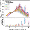Fig. 4. CO SLED and its evolution with redshift. Points have been shifted in the x-axis for clarity. The transition used for normalization is Jup = 3. Colors encode the redshift, from z = 0.5 to 3.0. In the upper panel, solid lines and shaded areas are the mean and 1σ deviation of the background SLED from the SIDES-Uchuu catalog. Points are obtained from Eq. (15) (and thus from the ratio of clustering power spectra) and the associated error bars from the dispersion over the 12 subfields of 9 deg2. The lower panel shows the relative difference between the mean SLED from the catalog and the measurement from the cross-power spectra.

The latter agrees within the 1-σ error bars with the mean SLED for J_up ≤ 6 at all redshifts. Over all the redshifts, J_up = 1, 2, 4, 5, 6, and 8 have a relative difference with respect to the mean SLED of 3 ± 14%, 4 ± 17%, 7 ± 19%, 7 ± 20%, 22 ± 32%, and 75 ± 85%, respectively. The relative difference tends to be larger in the z = 0.5 bin due to the smaller cosmic volume probed at lower redshift.

Furthermore, the CO(8–7) line is intrinsically faint, leading to non-detection of its clustering signal in two subfields at z = 0.5. Hence, we set an upper limit for R₃⁸(z = 0.5) in Fig. 4.

In addition, we can see that the relative difference evolves with J_up. This evolution is linked to the two-star-formation-mode model upon which the SIDES simulation is based, as detailed in Sect. 4.1.1. The peculiar case of CO(7–6), which is overestimated by a factor of ∼2, is discussed in Sect. 4.1.2.

4.1.1. Starbursts contribution to the background intensities

The SIDES model is built upon a two-star-formation-mode model from Sargent et al. (2012). The catalog contains MS and starburst (SB) galaxies, with an evolving fraction of SB galaxies from z = 0 to 1 as indicated by the black solid line and the right axis in Fig. 5. The left axis of Fig. 5 shows the contribution of SB to the mean CO background intensities as a function of redshift.

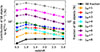Fig. 5. Left axis and colored dashed curves: Starburst’s contribution to mean brightness of transitions, as function of redshift up to Jup = 8, inferred from the SIDES-Uchuu catalog. Right axis and solid black curve: Starburst fraction in SIDES catalog.

We first examined the evolution of the SB contribution with J_up. SB have distinct CO SLED templates compared to MS galaxies, resulting in the SB having a stronger CO emission for J_up > 5 at fixed stellar and gas mass. Thus, the SB fractional contribution to the background is higher with increasing J_up. Although SB galaxies account for at most 3% of the galaxies in SIDES, their contribution to J_up ≤ 5 background intensities is between 3 and 10% over z = 0.5–3.0. For J_up = 6–8, their contribution rises to 13 ± 3, 20 ± 4, and 31 ± 5%, respectively, on average over z = 0.5–3.0. The low abundance of SB galaxies, combined with their large contribution to the J_up = 6–8 brightness, leads to the larger variance observed in these CO transition intensities.

Regarding the evolution of the SB contribution with redshift, it reaches its maximum at z = 1 for all transitions. Below z = 1, the decrease in the SB fraction results in a reduced SB contribution. Above z = 1, the SB contribution also decreases with increasing redshift, although the SB fraction remains constant and the SB emission template remains fixed with redshift. However, the MS template evolves with z, exhibiting higher excitation. As a result, the SB contribution is lower because the MS galaxies emit more.

We note that only selecting MS galaxies in the catalog would not eliminate the SB contribution in the measured cross-spectra, as the remaining galaxies still trace the large-scale structures where SBs reside. Given the significant contribution of these galaxies to the B_ν^{CO, J_up > 5}, it is important to give a careful interpretation in terms of global properties, unless these sources can be masked out of the CO maps.

We observe that SB galaxies have no reason to enhance or contribute differently to the effective clustering bias, b_eff. In SIDES, SB and MS star formation modes are randomly assigned to galaxies that are already clustered. Observationally, Béthermin et al. (2014) analyzed COSMOS data and concluded that MS and SB galaxies with the same stellar mass exhibit the same clustering bias and likely reside in halos of similar mass.

4.1.2. CO(7–6) contamination by [C_I](2–1)

Figure 4 shows that the excitations derived for CO(7–6) are largely overestimated at all redshifts. This is caused by the presence of the [C_I](2–1) line, which originates from the same redshifts and contributes to the cross-power amplitude. On average, between z = 0.5 and z = 3, [C_I] contributes 52% to the total measured background intensity, with weak evolution across the studied redshift range. Even if the two lines could be resolved, they would still be very close in redshift, practically tracing the same structures. Therefore, cross-correlation could not disentangle the two signals.

In summary, the cross-power spectrum method performs well to retrieve the CO background SLED with ≤20% uncertainty (up to z = 3.0 and J_up = 6). The next step is to derive the bias-weighted intensities, which are proportional to ρ_H2.

4.2. Effective bias-weighted intensities

From Eq. (5), the mean CO-line background intensity weighted by the effective clustering bias of CO emitters can be obtained from the simulation-based measured cross-power spectrum:

$$\begin{array}{c}\hfill B_{\nu }^{{\mathrm{J}}_{\mathrm{up}}}(z)b_{\mathrm{eff}}(z)=\frac{P_{{\mathrm{J}}_{\mathrm{up}}-\mathrm{gal}}^{\mathrm{clust}}(k_{\theta },z)}{b_{\mathrm{gal}}^{\mathrm{SIDES}}(z)\times P_{\mathrm{matter}}^{2\mathrm{D}}(k_{\theta },z)},\end{array}$$(16)

where $P_{{\mathrm{J}}_{\mathrm{up}}-\mathrm{gal}}^{\mathrm{clust}}(k,z)$ is the clustering component (k < 0.35 Mpc⁻¹) of the simulation-based cross-power spectrum of interloper-contaminated CO maps.

Figure 6 shows the resulting mean bias-weighted intensities obtained from the cross-power spectra. The color-code corresponds to each CO rotational level (up to J_up = 8). Solid lines and shaded areas show the mean and 1σ dispersion from the 12 subfields, respectively.

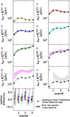Fig. 6. CO bias-weighted intensities as function of redshift. The color-code stands for the transitions’ Jup from 1 to 8. Solid lines and shaded areas correspond to the mean and 1σ dispersion, respectively, on the measured bias-weighted intensities from the 12 9 deg2 fields. Black dotted stars show the mean brightness derived analytically times the SIDES effective clustering bias $b_{\mathrm{eff}}^{\mathrm{fit}}$. The last panel in the left column shows the relative difference between the simulation-based and analytic bias-weighted intensities (i.e., the relative difference between colored lines and stars).

For a sanity check, the simulation-based bias-weighted intensities are compared to intrinsic values and displayed with stars in Fig. 6. The intrinsic values of B_ν^Jup(z) are obtained from Eq. (2) using the CO flux densities. The bias, b_eff^fit, is estimated from the CO line’s auto-power spectra, as described in Sect. 3.4. They constitute “interloper-free” estimates of the bias-weighted intensities in SIDES. The lower panel of the left column in Fig. 6 shows the relative difference between the simulation-based and intrinsic values. Apart from CO(7–6), already discussed in Sect. 4.1.2, simulation-based measured b_eff × B_ν at z > 0.5 agree with the analytical bias weighted intensities within their 1σ uncertainty.

For J_up = 1–5, the 1σ uncertainties on b_eff × B_ν(z > 0.5) from the cross-correlation method are ±10%. The uncertainties in the z = 0.5 bin are larger, from 10 to 20%, because this bin probes a smaller cosmic volume. Uncertainties rise to 15–20% for J_up = 6. Regarding CO(8–7), we set an upper limit for $b_{\mathrm{eff}}\times B_{\mathrm{eff}}^{\mathrm{CO}(8-7)}$ at z = 0.5 in Fig. 6 because, as discussed in the previous section, the CO(8–7) cross-spectrum is not detected in two subfields.

At z ≥ 1, $b_{\mathrm{eff}}\times B_{\nu }^{\mathrm{CO}(8-7)}$ appears to be overestimated by less than 1σ and shows a variance exceeding 30%, which is significantly higher than for the other lines. This overestimation is not significant, and it is due to the intrinsic faintness of the CO(8–7) background combined with significant contamination by the other CO lines and the bright [CII] line, which introduces a substantial level of interloper-induced noise. The remaining CO transitions are less affected by [CII] interlopers because of their higher intrinsic brightness. In contrast, the similarly faint CO(1–0) line remains unaffected by [CII] because the latter from z_[CII] ≥ 15 is too faint. In summary, the cross-power-spectrum method effectively recovers the bias-weighted intensities, except for CO(7–6), which is impacted by contamination from [CI].

4.3. Determination of the effective bias when the background is known

We next evaluate our ability to extract the effective bias, b_eff, from the interloper-contaminated cross-power spectra, given prior knowledge of the background intensities, B_ν^J_up. For this analysis, we assumed that the background level is known from line surveys, although this is typically not the case. Using this information, the goal is to test whether the effective bias can be recovered from the interloper-contaminated cross-power spectra.

The cross-power spectra are fit in a manner analogous to the auto-power spectra for each CO line, incorporating the known galaxy bias, b_gal, and their background intensity, B_ν. We then compare the cross-power-derived values of b_eff(z) with those obtained from the auto-power spectra, assessing their consistency and their ability to distinguish among different clustering bias models.

For the model, we used the halo bias model of Tinker et al. (2010, hereafter T10) to compute effective bias:

$$\begin{array}{c}\hfill b_{\mathrm{eff}}(z)=\frac{\int dMn(M,z)b_h^{\mathrm{T}10}(M,z)S_{\nu }(M,z)}{\int dMn(M,z)S_{\nu }(M,z)},\end{array}$$(17)

where b_h(M, z) is the halo clustering bias, and we used its Python implementation from the Colossus package (Diemer 2018).

We note that the derivation of the analytic clustering bias (Eq. (17)) makes use of the flux densities, S_ν, of the SIDES catalog. Thus, any discrepancy between the auto-power-based and analytic values of b_eff reflects the differences between the Uchuu simulation coupled with the abundance-matching procedure of SIDES and the halo-bias model of Tinker et al. (2010), which was calibrated on different simulations.

For all three estimates (from auto-power, cross-power, and Eq. (17)), the effective bias is the same whatever the CO line (within 3%), and it is shown as a function of redshift in Fig. 7. The consistency of the effective bias across different CO lines, despite the scatter in the SLED of galaxies (see Sect. 2.2), supports the assumption made in Eq. (15).

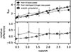Fig. 7. Effective bias of CO-emitters as function of redshift. The points have been slightly shifted in the x-axis for clarity. In the upper panel, stars represent the values fit from the CO auto-power without contamination, as described in Sect. 3.4. Gray triangles are obtained from the fit of interloper-contaminated cross-power spectra between CO LIM and galaxies. Pentagons show the values obtained via the analytic computation using Eq. (17) and the halo bias model of Tinker et al. (2010). Values are reported in Table. A.1. Lower panel shows the relative difference with the auto-power-based values of the bias.

At z = 0.5, the analytic clustering bias is 18% lower than the SIDES clustering bias. It rises more rapidly and exceeds the SIDES clustering bias at a turnover redshift of approximately z = 1.5. At z = 3, the analytic clustering bias is 14% higher than the SIDES clustering bias.

As expected, the error bars on the cross-power-based estimate of b_eff are larger due to the interlopers acting as a source of noise, but they agree within their 1-σ uncertainty with both the auto-power-based estimate and the analytic computation of the effective bias. Thus, the cross-power method is not inherently biased by interloper contamination; however, their presence limits its ability to constrain the bias model.

4.4. Cold-gas cosmic density

We now combine our previous results to estimate the cosmic density of cold gas, ρ_H2(z), and track its evolution with redshift. Converting CO luminosity densities to ρ_H2(z) implies the use of a global CO-to-H₂ mass conversion factor, ${\alpha }_{\mathrm{CO}}$. However, the value of ${\alpha }_{\mathrm{CO}}$ is known to vary with galaxy properties such as metallicity and environment, especially at high redshift. In addition, it tends to be lower in starbursts than in main-sequence galaxies (e.g., Downes & Solomon 1998). As a result, the contributions of different galaxy populations to ρ_H2 depend on their respective abundances, luminosities, and the assumed ${\alpha }_{\mathrm{CO}}$. This introduces an additional layer of degeneracy in the determination of ρ_H2.

Here, we assign different ${\alpha }_{\mathrm{CO}}$ conversion factors to MS galaxies and starbursts. With this simplified hypothesis, we can test the possibility to recover the gas density from a signal mixing the two populations with different ${\alpha }_{\mathrm{CO}}$. For this exercise, the total molecular gas density we aim to constrain is given by

$$\begin{array}{c}\hfill {\rho }_{\mathrm{H}2}(z)={\rho }_{L\prime }^{\mathrm{CO}(1-0),\mathrm{MS}}(z)\times {\alpha }_{\mathrm{CO}}^{\mathrm{MS}}+{\rho }_{L\prime }^{\mathrm{CO}(1-0),\mathrm{SB}}(z)\times {\alpha }_{\mathrm{CO}}^{\mathrm{SB}},\end{array}$$(18)

where ${\alpha }_{\mathrm{CO}}^{\mathrm{MS}}=4.0$ and ${\alpha }_{\mathrm{CO}}^{\mathrm{SB}}=0.8$ in units of M_⊙(K km s ⁻¹ pc²)⁻¹ are the conversion factors for MS galaxies and starbursts, respectively. The terms ${\rho }_{L\prime }^{\mathrm{CO}(1-0),\mathrm{MS}}(z)$ and ${\rho }_{L\prime }^{\mathrm{CO}(1-0),\mathrm{SB}}(z)$ are the pseudo-luminosity densities of CO(1–0) for these two populations. We computed the molecular gas density and its dispersion from the 12 9-deg² fields using the SIDES-Uchuu catalog. This computation provides us with a reference to test the accuracy of our method.

To obtain the simulation-based estimates of ρ_H2 from cross-spectra, we combined the simulation-based data obtained in Sects. 4.1 and 4.2, focusing on transitions with J_up > 1. We began by dividing the bias-weighted CO intensities by the effective clustering biases, as derived from the auto-power spectra in Sect. 4.2. This step yields the absolute CO background intensities. We then converted these intensities to the equivalent J_up, ref = 3 intensities using excitation ratios derived in Sect. 4.1.

Finally, the last step in the ρ_H2 determination for millimeter-wavelength LIM experiments is be to make an assumption about the excitation ratio, ${\mathrm{R}}_{{\mathrm{J}}_{\mathrm{up},\mathrm{ref}}-1,}$ between the reference transition (here J_up = 3) and J_up = 1 (the latter only being accessible at smaller frequencies with experiments such as COMAP).

We adopted the excitation ratio R₃₋₁ from SIDES, which has a value of 2.7 at z = 0.5 and increases linearly by 33% between z = 0.5 and z = 3.0. This ratio was then used to convert CO(3–2) intensities into their CO(1–0) equivalents.

The resulting estimates of ρ_H2 are shown in Fig. 8 as a function of redshift. For comparison, the intrinsic molecular gas density from Eq. (18) is indicated by the gray dashed line in each panel. Transitions with J_up = 7 and 8 are excluded from the analysis due to contamination by CI and high variance, respectively. The top left panel, where points are offset in the x-axis for clarity, shows the relative difference of ρ_H2 obtained from the simulation-based cross-spectrum estimates and from our reference computed using Eq. (18).

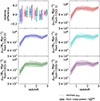Fig. 8. Cold-gas cosmic density, ρH2, as a function of redshift. The gray dashed curve in each panel is the intrinsic ρH2 from Eq. (18). Colored solid lines are the simulation-based estimate of ρH2 derived from the CO[Jup > 1] galaxy cross-spectra. The top left panel shows the relative difference from the intrinsic ρH2.

The mean relative difference between the simulation-based estimates and the reference ρ_H2(z) values does not exceed 7% for CO transitions from J_up = 2 to 6 at all redshifts. The 1-σ uncertainties of the relative difference are lower than 20% for J_up = 2–6, showing only a weak dependence on J_up.

We observe that uncertainties are lower for J_up = 3 (the reference transition), as it does not require estimating excitation ratios relative to higher transitions. The redshift evolution of the CO(3–2) background intensity is similar to that of CO(2–1) and CO(4–3). Thus, changing the reference transition would result in larger uncertainties in the CO(3–2)–based estimates, making them comparable to those derived from CO(2–1) or CO(4–3).

Regarding the influence of SB, the previous section of this paper shows that SB contribution to the background intensity increases with J_up. However, this contribution (which could lead to an overestimation of ρ_H2 by boosting the background intensity) is already taken into account in the mean (MS + SB) SLED and so is naturally corrected. The contribution of SB to ρ_H2 is less than 1% and is thus completely negligible compared to that of MS galaxies. However, we emphasize that the SB contribution scales with ${\alpha }_{\mathrm{CO}}^{\mathrm{SB}}$, which remains largely uncertain at high redshifts. Overall, the cross-correlation method with upper CO transitions can constrain the evolution of ρ_H2(z) to within 20%.

Since LIM is sensitive to the integral over the luminosity function, this observational method can bring complementary constraints to line surveys, which are sensitive to the brightest galaxies and rely on extrapolations to account for the faint end of the luminosity function. Data from the (sub)millimeter LIM in particular can complement the CO(1–0) LIM survey. Through cross-correlation, they can be used to constrain the SLED of the CO background across different redshifts. Finally, in combination with measurements of the CO(1–0) background, the CO-background SLED offers a valuable opportunity to estimate a “cosmic-averaged” gas-to-mass conversion factor, α_CO, and its redshift evolution.

5. Required sensitivity

Although current LIM experiments typically cover the fields smaller than 9 deg² considered above, a survey over 1.5 deg² can still, in principle, probe the same linear-scale regime. For instance, a CONCERTO-like experiment over 1.5 deg² can measure the power spectrum up to k_θ > 0.011 arcmin⁻¹, corresponding to k > 0.05 Mpc⁻¹ at z = 1.0.

CONCERTO completed its observations at APEX in December 2022, and data reduction of the COSMOS field is currently in progress. An estimate of the on-sky noise-equivalent intensity (NEI) for the spectroscopic mode will become available once this process is finalized, which will in turn enable predictions of the signal-to-noise ratio (S/N) for the CO × galaxy cross-correlation based directly on observational data.

To assess the feasibility of the previous analysis with a CONCERTO-like experiment, we estimated the sensitivity required to detect the CO LIM × galaxy spectroscopic survey cross-power signal, and compare it with the CONCERTO NEI reported in CONCERTO Collaboration (2020) and updated using the instrument characteristics measured on sky (Hu et al. 2024). CONCERTO has two detector arrays, a first array for low frequencies (LFs) and a second array for high frequencies (HFs). We took the LF array parameters for frequencies below 195 GHz and the HF parameters at higher frequencies.

In the above analysis, the cross-power spectrum is measured in two dimensions, first for each individual frequency channel (i.e., redshift slice), and then averaged over five channels. It is well suited because the SIDES simulation offers large fields, dominated by signal. Nevertheless, this 2D estimator is suboptimal with respect to a spherical cross-power that exploits the full set of available modes.

Thus, we determined the NEI requirements for spherical power spectra and examined whether they could be realistically achieved with a CONCERTO-like experiment. The required NEI to make a significant detection of the cross-power in the two-halo-dominated regime with a given S/N is:

$$\begin{array}{c}\hfill \mathrm{NEI}=b_{\mathrm{eff}}{B}_{\nu }^{{\mathrm{J}}_{\mathrm{up}}}\frac{\sqrt{t_{\mathrm{survey}}{N}_{\det }{N}_{\mathrm{spec}}}}{\sqrt{2}\pi \mathrm{S}/\mathrm{N}}{\left({\displaystyle {\int }_{k_{min}}^{k_{max}}{k}^2{P}_{\mathrm{matter}}^{3\mathrm{D}}(k)\mathrm{d}k}\right)}^{1/2}\end{array}$$(19)

with k_min = 0.1 Mpc⁻¹ and k_max = 0.35 Mpc⁻¹, which corresponds to the range relevant to the analysis of the previous sections. In this equation, N_det and N_spec are the number of detectors on the sky for each of the N_spec frequency channels of the LIM experiment. The term t_survey is the total integration time of the LIM survey.

The formalism to derive this equation is presented in Appendix B for a LIM experiment in which the underlying signal is dominated by instrument noise in individual voxel, such as CONCERTO. Here, we focus on the CO(4–3) line, which is covered over a wide redshift range by CONCERTO. The other two bright lines, CO(5–4) and CO(6–5), are discussed in Appendix B.

The adopted redshift bins to compute N_spec in Eq. (B.5) span Δz = 0.5, except at z = 0.5 and z = 2.5, where narrower bins of Δz = 0.23 and 0.32 are adopted, respectively, to take into account that the CONCERTO bandpass does not cover the full redshift bin. At CONCERTO’s spectral resolution of δν = 1.5 GHz, the radial modes are not sampled up to the full k_max = 0.35 Mpc⁻¹ range. Therefore we also computed the required NEI taking into account this loss in radial modes. The upper bound of the integration, k_max, becomes the larger k mode accessible by an instrument of resolution δν = 1.5 GHz at ν (see Eq. (B.15)). It ranges from k_max = 0.26 Mpc⁻¹ at z = 0.5 to k_max = 0.13 Mpc⁻¹ at z = 2.5.

Figure 9 shows the NEI required to detect the CO × galaxy cross-power signal at an S/N of three, together with the estimated CONCERTO NEI. We show two extreme cases of the NEI in this figure. In the first case (dashed green curve), we assumed that all the modes are recovered in the k-range of interest, neglecting the resolution effect. In the second case (solid blue line), we consider that all k larger than the resolution scales are lost, thus neglecting the contribution of transverse and potentially diagonal modes that could be recovered.

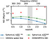Fig. 9. NEI required to detect CO(4–3) x-galaxy cross-power with a CONCERTO-like survey at an S/N of 3. The green dashed line corresponds to the NEI needed to detect the spherically averaged cross-power spectrum across the entire k range, [0.1–0.35] Mpc−1, computed using SIDES. The blue line represents the NEI requirement after accounting for the loss of modes imposed by CONCERTO’s spectral resolution of δν = 1.5 GHz. Estimates for CONCERTO’s NEI based on CONCERTO Collaboration (2020) and updated with on-sky instrument characteristics from Hu et al. (2024) are shown in red.

Our results show that CONCERTO’s sensitivity is insufficient to constrain the CO(4–3) cross-power, even under optimistic assumptions such as the availability of a spectroscopic galaxy survey (not yet available in the COSMOS field). Around z ∼ 1.5, the presence of a strong atmospheric water line at 183 GHz severely limits ground-based observations.

Our findings draw a consistent picture with the Tomographic Ionized-carbon Mapping Experiment (TIME) forecast by Sun et al. (2021), which predicts high S/N values for the CO × galaxy cross-power under the assumption that TIME reaches a NEI of 5 MJy sr⁻¹ s^−1/2, which is an order of magnitude lower than that required for a CONCERTO-like experiment (Fig. 9). Adopting the rest of their survey parameters for CO(4–3) at z = 1.0, N_feed ≡ N_det = 32, t_survey = 1000 h, and taking into account the two-halo term of the clustering in the [0.29–28] Mpc⁻¹k-range (similarly to that in Sun et al. 2021), we obtain a high S/N of 90. It is larger than the S/N of 17 that they reported, but the computation in Sun et al. (2021) takes into account the decorrelation caused by the redshift uncertainty of the galaxy survey (see the discussion in Sect. 2.5).

Our results also illustrate how the mode loss impacts the S/N, and consequently, the required NEI. Mode loss due to spectral resolution significantly decreases the goal NEI (solid blue curve), by a factor of ∼2 at z = 0.5 and 10 at z = 2.5, compared to when the full k-range is exploited (dashed green curve). It highlights that in this noise-dominated regime, fully exploiting all modes (both along and across the line of sight) can significantly boost the S/N of an LIM survey. Thus, to get the most out of cross-correlation, LIM surveys should be designed to sample their scales of interest in the three dimensions well.

6. Conclusion

This study explored the potential of the cross-correlation method between simulated millimeter-line-intensity mapping (millimeter-LIM) data and spectroscopic galaxy surveys to constrain the CO background SLED and the cosmic cold-gas density ρ_H2(z) from J > 1 CO transitions up to z = 3.0. The study used SIDES-Uchuu simulations, which offer an optimal compromise between large field coverage and detailed astrophysical modeling.

We used 12 light cones of 9 deg² extracted from the SIDES-Uchuu simulation. For each subfield, angular-spectral cubes of CO line intensity were built at six redshifts (from z = 0.5 to 3.0 by step of 0.5) as well as the galaxy (density contrast) cubes for a spectroscopic-like survey. We tested the impact of variance induced by interlopers, which can affect the accuracy of the results. Cross-correlation was then performed between each pair of interloper-contaminated CO intensity cube and corresponding galaxy overdensity cube, and the simulation-based angular cross-power spectrum was measured. The results for each redshift and CO transition were then averaged over the 12 subfields.

By analyzing the ratio of two cross-power spectra at different frequencies corresponding to the same redshift for two different CO transitions, the bias and scale-dependent factors can be simplified, enabling constraints on the CO background SLED. This in turn offers valuable insights into the molecular gas density and the physical conditions of the ISM in galaxies. Our main results are as follows:

• We show that the method is effective in retrieving the CO background SLED and the bias-weighted intensities up to z = 3.0 and J_up = 6. For the SLED, 1σ uncertainties are ≤20%. The 1σ uncertainties on b_eff × B_ν at z > 0.5 are of ± ∼ 10% for J_up = 1 to 5. This constraint rises to 15–20% for J_up = 6 and to > 30% for J_up = 8.

• CO(7–6) is intrinsically contaminated by [CI], and CO(8–7) appears poorly constrained due to the high dispersion induced by the high interloper contamination.

• We find that the effective biases between the different CO lines are the same. Thus, we took the ratio of two CO lines’ cross-power spectra corresponding to the same redshift in order to study the global excitation of the CO background.

• By combining the results on the CO background SLED and the bias-weighted intensities, we estimated the cosmic density of cold gas ρ_H2(z) and track its evolution with redshift. The 1σ relative uncertainties are lower than 20% for J_up = 2 to 6.

• Based on the two-star-formation-mode model of SIDES, we show that the rare starbursts (≥3% up to z ≤ 3) contribute more than 10% to the background intensity of transitions with J_up ≥ 6 (substantially increasing the variance in their cross-power and limiting their interpretation).

These results demonstrate the effectiveness of the cross-correlation method in isolating line emissions. It also provides important insights into the CO foreground of [CII] above z ≥ 6, which carries valuable information about star formation in early galaxies (e.g., Liu et al. 2024). This method can bring complementary constraints to the cosmic cold-gas density inferred from CO(1–0), as using the upper CO transitions allows one to constrain a wider range of redshifts from the same LIM dataset.

Our results show that the clustering of the CO cross galaxies power spectrum remains out of reach of a CONCERTO-like experiment in its current configuration. Nonetheless, we also show that leveraging the whole Fourier space, both in the radial and transverse direction to the line of sight, can significantly boost the S/N. It is thus important for a LIM experiment dominated by instrument noise component to sample the scales of interest in the three dimensions sufficiently.

In conclusion, the cross-correlation approach presented here has the potential to improve our understanding of the CO background SLED and the cosmic cold-gas density. It also opens new avenues for using upcoming CO LIM data to probe the interstellar medium and study its role in galaxy evolution.

References

Appendix A: Effective bias

Table A.1 reports the effective bias values from Fig. 7. The first column lists the values obtained analytically using Eq.,17 together with the halo bias model of Tinker et al. (2010). The second column shows the values fitted from the interloper-contaminated CO cross-power, and the third column those fitted from the contamination-free CO auto-power.

Appendix B: Sensitivity formalism

In this appendix, we describe the formalism used to compute the sensitivity required to detect the large-scale (linear regime) correlation between galaxy surveys and the CO mapped by a CONCERTO-like experiment. This sensitivity is usually expressed in terms of net equivalent intensity (NEI). In the following equations, the redshift dependence of the variables is neglected for simplicity. This approximation holds if the redshift slice is sufficiently narrow, such that galaxy evolution within it remains negligible. We then apply this formalism to the CO(4-3), CO(5-4) and CO(6-5) lines, which are the brightest lines in the SLED of Fig.4.

Appendix B.1: White-noise power spectrum

The white-noise power spectrum in a LIM dataset is typically expressed as:

$$\begin{array}{c}\hfill {\mathrm{P}}^{\mathrm{noise}}={\mathrm{V}}_{\mathrm{voxel}}\frac{{\mathrm{NEI}}^2}{{\mathrm{t}}_{\mathrm{int}}},\end{array}$$(B.1)

where V_voxel is the comoving volume corresponding to a single voxel (i.e., an element of the spatial–spectral cube), t_int is the effective integration time spent on that voxel and the last term is the NEI per detector, which for CONCERTO is frequency dependent.

Assuming that the LIM experiment observes with an instantaneous field of view Ω_inst, in which each detector covers one beam of solid angle Ω_beam, the integration time per voxel can be written as:

$$\begin{array}{c}\hfill {\mathrm{t}}_{\mathrm{int}}={\mathrm{t}}_{\mathrm{survey}}\frac{{\mathrm{\Omega }}_{\mathrm{inst}}}{{\mathrm{\Omega }}_{\mathrm{survey}}}={\mathrm{t}}_{\mathrm{survey}}\frac{{\mathrm{N}}_{\det }{\mathrm{\Omega }}_{\mathrm{beam}}}{{\mathrm{\Omega }}_{\mathrm{survey}}}={\mathrm{t}}_{\mathrm{survey}}\frac{{\mathrm{N}}_{\det }}{{\mathrm{N}}_{\mathrm{beam}}},\end{array}$$(B.2)

where the term t_survey is the total integration time on the field and the term N_beam = Ω_survey/Ω_beam is the number of independent beams in the LIM field.

If we approximate that the comoving volume per voxel, V_voxel, is constant with redshift, it can therefore be expressed as:

$$\begin{array}{c}\hfill {\mathrm{V}}_{\mathrm{voxel}}={\mathrm{V}}_{\mathrm{survey}}\frac{1}{{\mathrm{N}}_{\mathrm{beam}}{\mathrm{N}}_{\mathrm{spec}}},\end{array}$$(B.3)

where the comoving volume V_survey between (z_min and z_max) used to measure the cross-power is:

$$\begin{array}{c}\hfill {\mathrm{V}}_{\mathrm{survey}}=\frac{{\mathrm{\Omega }}_{\mathrm{survey}}}{3}[{\mathrm{D}}_{\mathrm{c}}^3({\mathrm{z}}_{max})-{\mathrm{D}}_{\mathrm{c}}^3({\mathrm{z}}_{min})],\end{array}$$(B.4)

We further define Δz as z_max − z_min.

The N_spec factor corresponds to the number of independent spectral elements within the redshift bin Δz and can be computed using:

$$\begin{array}{c}\hfill {\mathrm{N}}_{\mathrm{spec}}=({\nu }_{\max }^{\mathrm{z}-\mathrm{bin}}-{\nu }_{\min }^{\mathrm{z}-\mathrm{bin}})/\delta \nu ,\end{array}$$(B.5)

where δν is the spectral resolution of the instrument.

Combining the previous equations, we can obtain another expression of the noise auto-power spectrum:

$$\begin{array}{c}\hfill {\mathrm{P}}^{\mathrm{noise}}={\mathrm{V}}_{\mathrm{survey}}\frac{{\mathrm{NEI}}^2}{{\mathrm{t}}_{\mathrm{survey}}}\frac{1}{{\mathrm{N}}_{\det }{\mathrm{N}}_{\mathrm{spec}}}\end{array}$$(B.6)

Appendix B.2: Signal-to-noise ratio

Reaching a significance in the detection of the cross-power spectrum, given the survey parameters, implies a required NEI. Here, we want to derive the NEI required to detect the cross-power spectrum between a CO line and a galaxy spectroscopic survey (which is defined in Sect. 2) at a given S/N over the scales of interest.

We first compute the S/N obtained at a given scale considering all the modes between k and k+δk:

$$\begin{array}{c}\hfill \delta \mathrm{S}/\mathrm{N}(\mathrm{k})=\frac{{\mathrm{P}}_{{\mathrm{J}}_{\mathrm{up}}\times \mathrm{G}}(\mathrm{k})}{{\sigma }_{{\mathrm{J}}_{\mathrm{up}}}(\mathrm{k})}\end{array}$$(B.7)

where the denominator is the uncertainty in the LIM x Galaxies cross-power σ_Jup × G (Wolz et al. 2017):

$$\begin{array}{c}\hfill {\sigma }_{{\mathrm{J}}_{\mathrm{up}}}(\mathrm{k})=\frac{\sqrt{{\mathrm{P}}_{{\mathrm{J}}_{\mathrm{up}}\times \mathrm{G}}^2(\mathrm{k})+({\mathrm{P}}_{{\mathrm{J}}_{\mathrm{up}}}(\mathrm{k})+{\mathrm{P}}^{\mathrm{noise}}){\mathrm{P}}_{\mathrm{G}}(\mathrm{k})}}{\sqrt{2\delta {\mathrm{N}}_{\mathrm{modes}}(\mathrm{k})}}\end{array}$$(B.8)

The term δN_modes is the number of independent modes between k and k+δk.

Based on the discussion of Sect. 2.5, we assume that the spectroscopic survey, with dz/(1+z) ∼10⁻³, do not introduce an extra attenuation at the relevant scales. We note that using photometric surveys with dz/(1+z) ∼10⁻², available so far in COSMOS, would introduce an non-negligible attenuation of the cross-power amplitudes.

In the noise-dominated regime characteristic of current LIM experiments, we assume that each voxel is primarily affected by white noise, with only a weak underlying signal. Accordingly, we adopt the approximations P_noise > > P_J(k) and P_noiseP_G(k) > > P_J − G²(k). We verify a posteriori whether these assumptions hold.

The resulting goal NEI from these assumptions is the minimal sensitivity that a LIM instrument has to reach to obtain a significant detection. These assumptions simplify Eq. B.7 to:

$$\begin{array}{c}\hfill \delta \mathrm{S}/\mathrm{N}=\frac{{\mathrm{P}}_{{\mathrm{J}}_{\mathrm{up}}\times \mathrm{G}}(\mathrm{k})}{\sqrt{{\mathrm{P}}_{\mathrm{G}}(\mathrm{k})}}\frac{\sqrt{2\delta {\mathrm{N}}_{\mathrm{modes}}(\mathrm{k})}}{\sqrt{{\mathrm{P}}^{\mathrm{noise}}}}\end{array}$$(B.9)

At the relevant scales, the two-halo term of the clustering dominates. Thus, using Eq. 5 and Eq. 13, we can simplify the first factor in the previous equation:

$$\begin{array}{c}\hfill \frac{{\mathrm{P}}_{{\mathrm{J}}_{\mathrm{up}}\times \mathrm{G}}(\mathrm{k})}{\sqrt{{\mathrm{P}}_{\mathrm{G}}(\mathrm{k})}}={\mathrm{b}}_{\mathrm{eff}}{\mathrm{B}}_{\nu }^{{\mathrm{J}}_{\mathrm{up}}}\sqrt{{\mathrm{P}}_{\mathrm{matter}}^{3\mathrm{D}}(\mathrm{k})},\end{array}$$(B.10)

where ${\mathrm{b}}_{\mathrm{eff}}{\mathrm{B}}_{\nu }^{{\mathrm{J}}_{\mathrm{up}}}$is the CO line bias-weighted background intensity and $P_{\mathrm{matter}}^{3\mathrm{D}}(k)$ is the three-dimensional matter power spectrum, both assumed not to evolve significantly across the redshift bin. We use the value at the center of the redshift bin in our numerical computations.

To compute the total S/N, we sum quadratically the δS/N over all the relevant wavenumbers:

$$\begin{array}{c}\hfill {\mathrm{S}/\mathrm{N}}_{\mathrm{tot}}={\left[{\displaystyle \int \delta }{\mathrm{S}/\mathrm{N}}^2\mathrm{dk}\right]}^{1/2},\end{array}$$(B.11)

The resulting S/N_tot for a given [k_min, k_max] range is then:

$$\begin{array}{cc}\hfill {\mathrm{S}/\mathrm{N}}_{\mathrm{tot}}& =\sqrt{2}\frac{{\mathrm{b}}_{\mathrm{eff}}{\mathrm{B}}_{\nu }^{{\mathrm{J}}_{\mathrm{up}}}}{\sqrt{P^{\mathrm{noise}}}}{\left[{\displaystyle {\int }_{{\mathrm{k}}_{min}}^{{\mathrm{k}}_{max}}}\delta N_{\mathrm{modes}}(k){\mathrm{P}}_{\mathrm{matter}}^{3\mathrm{D}}(k)dk\right]}^{1/2}\hfill \\ \hfill & =b_{\mathrm{eff}}{B}_{\nu }^{J_{\mathrm{up}}}\frac{\sqrt{2{\mathrm{t}}_{\mathrm{survey}}{\mathrm{N}}_{\det }{\mathrm{N}}_{\mathrm{spec}}}}{\sqrt{{\mathrm{V}}_{\mathrm{survey}}}\mathrm{NEI}}\hfill \\ \hfill & \times {\left[{\displaystyle {\int }_{{\mathrm{k}}_{min}}^{{\mathrm{k}}_{max}}}\delta {\mathrm{N}}_{\mathrm{modes}}(\mathrm{k}){\mathrm{P}}_{\mathrm{matter}}^{3\mathrm{D}}(\mathrm{k})\mathrm{dk}\right]}^{1/2}\hfill \end{array}$$(B.12)

Equation B.12 indicates that achieving a specific S/N requires attaining a certain level of white noise, which in turn depends on the NEI. In the expression of the S/N, the noise level is balanced by the number of independent modes in the power spectrum measurement.

Given a fix integration time, for all survey sizes that have access to the same given k-range, assuming they have the same galaxy redshift quality, we expect to have the same S/N_tot. However, larger surveys can probe lower k values, thus providing larger S/N if computed using lower k_min.

Appendix B.3: NEI for spherical cross-power

In three-dimensional space, the number of independent modes between k and k+δk is given by:

$$\begin{array}{c}\hfill \delta {\mathrm{N}}_{\mathrm{modes}}=\frac{1}{2}\frac{{\mathrm{V}}_{\mathrm{survey}}}{{(2\pi )}^3}\times 4\pi {\mathrm{k}}^2\end{array}$$(B.13)

The 1/2 factor in the expression accounts for the Hermitian symmetry of the Fourier transform of real-valued fields, and considers only the modes in the positive half of the Fourier space. Combining all of the above, the NEI required to significantly detect the spherically averaged cross-power spectrum in the two-halo-dominated regime is:

$$\begin{array}{c}\hfill \mathrm{NEI}={\mathrm{b}}_{\mathrm{eff}}{\mathrm{B}}_{\nu }^{{\mathrm{J}}_{\mathrm{up}}}\frac{\sqrt{{\mathrm{t}}_{\mathrm{survey}}{\mathrm{N}}_{\det }{\mathrm{N}}_{\mathrm{spec}}}}{\sqrt{2}\pi \mathrm{S}/\mathrm{N}}{\left({\displaystyle {\int }_{{\mathrm{k}}_{min}}^{{\mathrm{k}}_{max}}}{\mathrm{k}}^2{\mathrm{P}}_{\mathrm{matter}}^{3\mathrm{D}}(\mathrm{k})\mathrm{d}\mathrm{k}\right)}^{1/2}\end{array}$$(B.14)

The integration is performed on scales of interest of this work, in which the linear clustering of galaxies dominates. The lower integration bound k_min, is 0.1 Mpc⁻¹, and the upper integration bound k_max, is 0.35 Mpc⁻¹.

For consistency, the k-range over which the integral is performed must be well sampled in both the transverse and radial directions to get an isotropic measurement. In the transverse direction, the smallest well-sampled scale (i.e. the largest accessible k) is set by the instrumental beam, and is much smaller than the linear scales used in our analysis. In contrast, in the radial direction, it is set by the spectral resolution. In the radial direction, the smallest scale is the comoving distance between two consecutive frequency channels. Thus, the upper integration bound k_max is given by:

$$\begin{array}{c}\hfill {\mathrm{k}}_{\max }=2\pi \frac{\mathrm{H}\nu }{\mathrm{c}(1+\mathrm{z})\delta \nu },\end{array}$$(B.15)

which, given the CONCERTO-like survey parameter, is smaller than the 0.35Mpc⁻¹ used in the main text. Accordingly, we also compute the NEI taking into account this loss of modes by changing the upper integration bound from 0.35 Mpc⁻¹ to the largest accessible mode of Eq. B.15.

Appendix B.4: CO(5-4) and CO(6-5) NEI

While the main text focuses on CO(4–3), Fig. B.1 presents the required NEI to detect the cross-power of two other lines: CO(5–4) and CO(6–5), within the CONCERTO frequency band. The redshift bins over which the target NEI is evaluated span Δz = 0.5, except at z = 0.5 and z = 2.5 for CO(4–3) and at z = 1.0 for CO(5–4). For these cases, the CONCERTO bandpass (130–310 GHz) does not cover the full redshift bin. Thus, we take narrower bins: Δz = 0.22 and 0.31 for CO(4-3) and Δz = 0.37 for CO(5-4), respectively, in order to match CONCERTO’s bandpass.

Overall, the brighter the line, the higher the required NEI, although the order of magnitude remains comparable among the main CO transitions. Consequently, CO(5–4), which corresponds to the peak of the SLED in Fig. 4, does not require a NEI as low as the two other transitions.

In particular, at z = 1.0, the required NEI is similar for CO(4–3) and CO(5–4), despite the latter being intrinsically brighter. This is due to CO(4–3) falling within the LF array, which has more valid detectors than the HF array hosting CO(5–4) at this redshift (see Table 2).

Appendix B.5: Validation of Assumptions

Using the parameters of Sect. 5 for a CONCERTO-like survey, we verify that the assumption P_noiseP_G(k) > > P_J − G²(k) holds. Given the expression of each term, this is equivalent to checking that ${\mathrm{P}}_{\mathrm{noise}}>>({\mathrm{b}}_{\mathrm{eff}}{\mathrm{B}}_{{\mathrm{J}}_{\mathrm{up}}}^{\nu }){\mathrm{P}}_{\mathrm{matter}}^{3\mathrm{D}}(\mathrm{k})$. Since the noise level depends on the area of the LIM survey, we take Ω_survey = 1.5 deg², consistent with the expected size of the CONCERTO field. The term ${\mathrm{P}}_{\mathrm{matter}}^{3\mathrm{D}}$ is evaluated at k = 0.1 Mpc⁻¹. Figure B.2 presents the numerical application. When the NEI is computed for the whole k-range [0.1,0.35] Mpc⁻¹, the term P_noiseP_G(k) is more than one order of magnitude above the cross-term P_J − G²(k). When taking into account the loss in radial modes due to the finite spectral resolution of a CONCERTO-like survey, P_noiseP_G(k) is a factor of ≥9 above the cross term, up to redshift z = 2. At redshift 2.5, P_noiseP_G(k) still dominates the cross term by a factor of 3, due to the important loss of modes (k_max = 0.13 Mpc⁻¹ at z = 2.5).

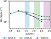Fig. B.1. Net equivalent intensity needed to detect the CO LIM cross-galaxies power spectrum at a S/N of 3, assuming an isotropic upper integration bound kmax = 0.35 Mpc−1. The color code stands for the CO(4-3), CO(5-4) and CO(6-5) lines, in blue, green and purple respectively. Colored areas indicate the redshifts contaminated by the 183 GHz atmospheric water line for each of the three CO lines.

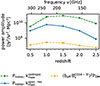Fig. B.2. Power amplitudes of the terms entering the expression of σJup − G(k) (Eq B.8). The orange dashed line shows the power amplitude of the cross-term $({\mathrm{b}}_{\mathrm{eff}}{\mathrm{B}}_{\nu }^{{\mathrm{J}}_{\mathrm{up}}}){\mathrm{P}}_{\mathrm{matter}}^{3\mathrm{D}}$. The green dashed line shows the white noise power amplitude integrated over the k-range 0.1-0.35 Mpc−1. In contrast, the blue solid line shows the white noise power amplitude integrated up to kmax defined in Eq. B.15. Overall, the condition ${\mathrm{P}}_{\mathrm{noise}}>>({\mathrm{b}}_{\mathrm{eff}}{\mathrm{B}}_{\nu }^{{\mathrm{J}}_{\mathrm{up}}}){\mathrm{P}}_{\mathrm{matter}}^{3\mathrm{D}}$ is verified, but when restricting the integral to the smallest accessible scale in the radial direction, PnoisePG exceeds the cross-term PJup × G only by a factor of a few.

All Tables

All Figures

	Fig. 1. Right axis: Mean number of galaxies per galaxy cube covering 9-deg2 and Δz = 0.25, as a function of redshift. The error bars come from the dispersion over the twelve independent light cones. Left axis: The associated shot noise of galaxy’s number density contrast in the 9-deg2 fields.
In the text

	Fig. 2. From left to right: Images of SIDES intrinsic CO(4–3) cube integrated along spectral axis over Δz = 0.25, the same CO(4–3) cube including contamination from line interlopers, and the galaxy cube integrated over the same redshift range. The top row corresponds to z = 0.5 and the bottom row to z = 3.0. Continuum contamination is assumed to have been removed beforehand.
In the text

Fig. 3. Upper panel: CO(4–3) auto-power spectrum at z = 0.5. The dashed gray line shows the simulation-based auto-power spectrum Ptot(k). It is the average over the five auto-power spectra of CO(4–3) maps, each map spanning δz = 0.05. The dotted gray line shows the average shot noise component. Subtracting the shot noise yields the clustering Pclust(k) shown with the solid gray line. The clustering (Eq. (11)) is fit to Pclust at large scales only, using the red points. From this fit, the effective clustering bias in SIDES, $b_{\mathrm{eff}}^{\mathrm{fit}}$, is estimated. Lower panel: Same procedure for galaxies’ auto-power spectra and $b_{\mathrm{gal}}^{\mathrm{fit}}$, still at z = 0.5.

In the text

Fig. 4. CO SLED and its evolution with redshift. Points have been shifted in the x-axis for clarity. The transition used for normalization is Jup = 3. Colors encode the redshift, from z = 0.5 to 3.0. In the upper panel, solid lines and shaded areas are the mean and 1σ deviation of the background SLED from the SIDES-Uchuu catalog. Points are obtained from Eq. (15) (and thus from the ratio of clustering power spectra) and the associated error bars from the dispersion over the 12 subfields of 9 deg2. The lower panel shows the relative difference between the mean SLED from the catalog and the measurement from the cross-power spectra.

In the text

	Fig. 5. Left axis and colored dashed curves: Starburst’s contribution to mean brightness of transitions, as function of redshift up to Jup = 8, inferred from the SIDES-Uchuu catalog. Right axis and solid black curve: Starburst fraction in SIDES catalog.
In the text

Fig. 6. CO bias-weighted intensities as function of redshift. The color-code stands for the transitions’ Jup from 1 to 8. Solid lines and shaded areas correspond to the mean and 1σ dispersion, respectively, on the measured bias-weighted intensities from the 12 9 deg2 fields. Black dotted stars show the mean brightness derived analytically times the SIDES effective clustering bias $b_{\mathrm{eff}}^{\mathrm{fit}}$. The last panel in the left column shows the relative difference between the simulation-based and analytic bias-weighted intensities (i.e., the relative difference between colored lines and stars).

In the text

Fig. 7. Effective bias of CO-emitters as function of redshift. The points have been slightly shifted in the x-axis for clarity. In the upper panel, stars represent the values fit from the CO auto-power without contamination, as described in Sect. 3.4. Gray triangles are obtained from the fit of interloper-contaminated cross-power spectra between CO LIM and galaxies. Pentagons show the values obtained via the analytic computation using Eq. (17) and the halo bias model of Tinker et al. (2010). Values are reported in Table. A.1. Lower panel shows the relative difference with the auto-power-based values of the bias.

In the text

	Fig. 8. Cold-gas cosmic density, ρH2, as a function of redshift. The gray dashed curve in each panel is the intrinsic ρH2 from Eq. (18). Colored solid lines are the simulation-based estimate of ρH2 derived from the CO[Jup > 1] galaxy cross-spectra. The top left panel shows the relative difference from the intrinsic ρH2.
In the text

Fig. 9. NEI required to detect CO(4–3) x-galaxy cross-power with a CONCERTO-like survey at an S/N of 3. The green dashed line corresponds to the NEI needed to detect the spherically averaged cross-power spectrum across the entire k range, [0.1–0.35] Mpc−1, computed using SIDES. The blue line represents the NEI requirement after accounting for the loss of modes imposed by CONCERTO’s spectral resolution of δν = 1.5 GHz. Estimates for CONCERTO’s NEI based on CONCERTO Collaboration (2020) and updated with on-sky instrument characteristics from Hu et al. (2024) are shown in red.

In the text

	Fig. B.1. Net equivalent intensity needed to detect the CO LIM cross-galaxies power spectrum at a S/N of 3, assuming an isotropic upper integration bound kmax = 0.35 Mpc−1. The color code stands for the CO(4-3), CO(5-4) and CO(6-5) lines, in blue, green and purple respectively. Colored areas indicate the redshifts contaminated by the 183 GHz atmospheric water line for each of the three CO lines.
In the text

Fig. B.2. Power amplitudes of the terms entering the expression of σJup − G(k) (Eq B.8). The orange dashed line shows the power amplitude of the cross-term $({\mathrm{b}}_{\mathrm{eff}}{\mathrm{B}}_{\nu }^{{\mathrm{J}}_{\mathrm{up}}}){\mathrm{P}}_{\mathrm{matter}}^{3\mathrm{D}}$. The green dashed line shows the white noise power amplitude integrated over the k-range 0.1-0.35 Mpc−1. In contrast, the blue solid line shows the white noise power amplitude integrated up to kmax defined in Eq. B.15. Overall, the condition ${\mathrm{P}}_{\mathrm{noise}}>>({\mathrm{b}}_{\mathrm{eff}}{\mathrm{B}}_{\nu }^{{\mathrm{J}}_{\mathrm{up}}}){\mathrm{P}}_{\mathrm{matter}}^{3\mathrm{D}}$ is verified, but when restricting the integral to the smallest accessible scale in the radial direction, PnoisePG exceeds the cross-term PJup × G only by a factor of a few.

In the text

References

- Beane, A., Villaescusa-Navarro, F., & Lidz, A. 2019, ApJ, 874, 133 [Google Scholar]
- Bernal, J. L., & Kovetz, E. D. 2022, A&ARv, 30, 5 [NASA ADS] [CrossRef] [Google Scholar]
- Béthermin, M., Daddi, E., Magdis, G., et al. 2012, ApJ, 757, L23 [Google Scholar]
- Béthermin, M., Kilbinger, M., Daddi, E., et al. 2014, A&A, 567, A103 [NASA ADS] [CrossRef] [EDP Sciences] [Google Scholar]
- Béthermin, M., Wu, H.-Y., Lagache, G., et al. 2017, A&A, 607, A89 [Google Scholar]
- Béthermin, M., Gkogkou, A., Van Cuyck, M., et al. 2022, A&A, 667, A156, (B22) [Google Scholar]
- Birkin, J. E., Weiss, A., Wardlow, J. L., et al. 2021, MNRAS, 501, 3926 [Google Scholar]
- Bolatto, A. D., Wolfire, M., & Leroy, A. K. 2013, ARA&A, 51, 207 [CrossRef] [Google Scholar]
- Boogaard, L. A., van der Werf, P., Weiss, A., et al. 2020, ApJ, 902, 109 [NASA ADS] [CrossRef] [Google Scholar]
- Boogaard, L. A., Decarli, R., Walter, F., et al. 2023, ApJ, 945, 111 [NASA ADS] [CrossRef] [Google Scholar]
- Bournaud, F., Daddi, E., Weiß, A., et al. 2015, A&A, 575, A56 [NASA ADS] [CrossRef] [EDP Sciences] [Google Scholar]
- Bradford, C. M., Aguirre, J. E., Aikin, R., et al. 2009, ApJ, 705, 112 [NASA ADS] [CrossRef] [Google Scholar]
- Breysse, P. C., Yang, S., Somerville, R. S., et al. 2022, ApJ, 929, 30 [NASA ADS] [CrossRef] [Google Scholar]
- Carilli, C. L., & Walter, F. 2013, ARA&A, 51, 105 [NASA ADS] [CrossRef] [Google Scholar]
- CCAT-Prime Collaboration (Aravena, M., et al.) 2023, ApJS, 264, 7 [NASA ADS] [CrossRef] [Google Scholar]
- Chabrier, G. 2003, PASP, 115, 763 [Google Scholar]
- Chung, D. T. 2023, JCAP, 2023, 024 [CrossRef] [Google Scholar]
- Chung, D. T., Viero, M. P., Church, S. E., et al. 2019, ApJ, 872, 186 [NASA ADS] [CrossRef] [Google Scholar]
- Cleary, K. A., Borowska, J., Breysse, P. C., et al. 2022, ApJ, 933, 182 [NASA ADS] [CrossRef] [Google Scholar]
- CONCERTO Collaboration (Ade, P., et al.) 2020, A&A, 642, A60 [NASA ADS] [CrossRef] [EDP Sciences] [Google Scholar]
- Crites, A. T., Bock, J. J., Bradford, C. M., et al. 2014, in Millimeter, Submillimeter, and Far-Infrared Detectors and Instrumentation for Astronomy VII, eds. W. S. Holland, & J. Zmuidzinas, SPIE Conf. Ser., 9153, 91531W [NASA ADS] [CrossRef] [Google Scholar]
- Daddi, E., Dannerbauer, H., Liu, D., et al. 2015, A&A, 577, A46 [NASA ADS] [CrossRef] [EDP Sciences] [Google Scholar]
- Danielson, A. L. R., Swinbank, A. M., Smail, I., et al. 2011, MNRAS, 410, 1687 [NASA ADS] [Google Scholar]
- Davidzon, I., Ilbert, O., Laigle, C., et al. 2017, A&A, 605, A70 [NASA ADS] [CrossRef] [EDP Sciences] [Google Scholar]
- De Looze, I., Cormier, D., Lebouteiller, V., et al. 2014, A&A, 568, A62 [NASA ADS] [CrossRef] [EDP Sciences] [Google Scholar]
- Decarli, R., Aravena, M., Boogaard, L., et al. 2020, ApJ, 902, 110 [Google Scholar]
- Diemer, B. 2018, ApJS, 239, 35 [NASA ADS] [CrossRef] [Google Scholar]
- Downes, D., & Solomon, P. M. 1998, ApJ, 507, 615 [NASA ADS] [CrossRef] [Google Scholar]
- Essinger-Hileman, T., Oxholm, T., Siebert, G., et al. 2020, in Millimeter, Submillimeter, and Far-Infrared Detectors and Instrumentation for Astronomy X, eds. J. Zmuidzinas, & J.-R. Gao, SPIE Conf. Ser., 11453, 114530H [Google Scholar]
- Genzel, R., Tacconi, L. J., Lutz, D., et al. 2015, ApJ, 800, 20 [Google Scholar]
- Gkogkou, A., Béthermin, M., Lagache, G., et al. 2023, A&A, 670, A16 [NASA ADS] [CrossRef] [EDP Sciences] [Google Scholar]
- Greve, T. R., Leonidaki, I., Xilouris, E. M., et al. 2014, ApJ, 794, 142 [NASA ADS] [CrossRef] [Google Scholar]
- Gururajan, G., Bethermin, M., Sulzenauer, N., et al. 2023, A&A, 676, A89 [NASA ADS] [CrossRef] [EDP Sciences] [Google Scholar]
- Harris, A. I., Baker, A. J., Zonak, S. G., et al. 2010, ApJ, 723, 1139 [NASA ADS] [CrossRef] [Google Scholar]
- Howlett, C., Lewis, A., Hall, A., & Challinor, A. 2012, JCAP, 2012, 027 [Google Scholar]
- Hu, W., Beelen, A., Lagache, G., et al. 2024, A&A, 689, A20 [NASA ADS] [CrossRef] [EDP Sciences] [Google Scholar]
- Ishiyama, T., Prada, F., Klypin, A. A., et al. 2021, MNRAS, 506, 4210 [NASA ADS] [CrossRef] [Google Scholar]
- Ivison, R. J., Papadopoulos, P. P., Smail, I., et al. 2011, MNRAS, 412, 1913 [Google Scholar]
- Kade, K., Knudsen, K. K., Bewketu Belete, A., et al. 2024, A&A, 684, A56 [NASA ADS] [CrossRef] [EDP Sciences] [Google Scholar]
- Karkare, K. S., Anderson, A. J., Barry, P. S., et al. 2022, J. Low Temp. Phys., 209, 758 [NASA ADS] [CrossRef] [Google Scholar]
- Karoumpis, C., Magnelli, B., Romano-Díaz, E., et al. 2024, A&A, 691, A262 [NASA ADS] [CrossRef] [EDP Sciences] [Google Scholar]
- Keating, G. K., Marrone, D. P., Bower, G. C., & Keenan, R. P. 2020, ApJ, 901, 141 [NASA ADS] [CrossRef] [Google Scholar]
- Keenan, R. P., Marrone, D. P., & Keating, G. K. 2020, ApJ, 904, 127 [NASA ADS] [CrossRef] [Google Scholar]
- Kennicutt, R. C., Jr. 1998, ARA&A, 36, 189 [Google Scholar]
- Kovetz, E. D., Viero, M. P., Lidz, A., et al. 2017, Phys. Rep., submitted [arXiv:1709.09066] [Google Scholar]
- Laigle, C., McCracken, H. J., Ilbert, O., et al. 2016, ApJS, 224, 24 [Google Scholar]
- Li, J., Wang, R., Riechers, D., et al. 2020, ApJ, 889, 162 [NASA ADS] [CrossRef] [Google Scholar]
- Liu, L.-J., Sun, G., Chang, T.-C., Furlanetto, S. R., & Bradford, C. M. 2024, ApJ, 974, 175 [Google Scholar]
- Lu, N., Zhao, Y., Díaz-Santos, T., et al. 2017, ApJS, 230, 1 [Google Scholar]
- Madau, P., & Dickinson, M. 2014, ARA&A, 52, 415 [Google Scholar]
- Magnelli, B., Boogaard, L., Decarli, R., et al. 2020, ApJ, 892, 66 [NASA ADS] [CrossRef] [Google Scholar]
- McKee, C. F., & Ostriker, E. C. 2007, ARA&A, 45, 565 [Google Scholar]
- Murmu, C. S., Majumdar, S., & Datta, K. K. 2021, MNRAS, 507, 2500 [NASA ADS] [CrossRef] [Google Scholar]
- Neben, A. R., Stalder, B., Hewitt, J. N., & Tonry, J. L. 2017, ApJ, 849, 50 [NASA ADS] [CrossRef] [Google Scholar]
- Padmanabhan, H., Breysse, P., Lidz, A., & Switzer, E. R. 2022, MNRAS, 515, 5813 [NASA ADS] [CrossRef] [Google Scholar]
- Péroux, C., & Howk, J. C. 2020, ARA&A, 58, 363 [CrossRef] [Google Scholar]
- Planck Collaboration XIII. 2016, A&A, 594, A13 [NASA ADS] [CrossRef] [EDP Sciences] [Google Scholar]
- Riechers, D. A., Hodge, J., Walter, F., Carilli, C. L., & Bertoldi, F. 2011, ApJ, 739, L31 [Google Scholar]
- Riechers, D. A., Pavesi, R., Sharon, C. E., et al. 2019, ApJ, 872, 7 [Google Scholar]
- Rosenberg, M. J. F., van der Werf, P. P., Aalto, S., et al. 2015, ApJ, 801, 72 [Google Scholar]
- Roy, A., & Battaglia, N. 2024, ApJ, 969, 2 [Google Scholar]
- Saintonge, A., Lutz, D., Genzel, R., et al. 2013, ApJ, 778, 2 [Google Scholar]
- Sargent, M. T., Béthermin, M., Daddi, E., & Elbaz, D. 2012, ApJ, 747, L31 [Google Scholar]
- Sargent, M. T., Daddi, E., Béthermin, M., et al. 2014, ApJ, 793, 19 [NASA ADS] [CrossRef] [Google Scholar]
- Schaan, E., & White, M. 2021, JCAP, 2021, 068 [CrossRef] [Google Scholar]
- Scoville, N., Lee, N., Vanden Bout, P., et al. 2017, ApJ, 837, 150 [Google Scholar]
- Silva, M. B., Kovetz, E. D., Keating, G. K., et al. 2021, Exp. Astron., 51, 1593 [Google Scholar]
- Sun, G., Chang, T. C., Uzgil, B. D., et al. 2021, ApJ, 915, 33 [NASA ADS] [CrossRef] [Google Scholar]
- Tacconi, L. J., Neri, R., Genzel, R., et al. 2013, ApJ, 768, 74 [NASA ADS] [CrossRef] [Google Scholar]
- Tacconi, L. J., Genzel, R., Saintonge, A., et al. 2018, ApJ, 853, 179 [Google Scholar]
- Tacconi, L. J., Genzel, R., & Sternberg, A. 2020, ARA&A, 58, 157 [NASA ADS] [CrossRef] [Google Scholar]
- Tinker, J. L., Robertson, B. E., Kravtsov, A. V., et al. 2010, ApJ, 724, 878 [NASA ADS] [CrossRef] [Google Scholar]
- Valentino, F., Magdis, G. E., Daddi, E., et al. 2018, ApJ, 869, 27 [Google Scholar]
- Valentino, F., Magdis, G. E., Daddi, E., et al. 2020, ApJ, 890, 24 [Google Scholar]
- Van Cuyck, M., Ponthieu, N., Lagache, G., et al. 2023, A&A, 676, A62 [NASA ADS] [CrossRef] [EDP Sciences] [Google Scholar]
- Viero, M. P., Wang, L., Zemcov, M., et al. 2013, ApJ, 772, 77 [Google Scholar]
- Visbal, E., & McQuinn, M. 2023, ApJ, 956, 84 [Google Scholar]
- Walter, F., Carilli, C., Neeleman, M., et al. 2020, ApJ, 902, 111 [Google Scholar]
- Weiß, A., Downes, D., Neri, R., et al. 2007, A&A, 467, 955 [NASA ADS] [CrossRef] [EDP Sciences] [Google Scholar]
- Whitaker, K. E., Williams, C. C., Mowla, L., et al. 2021, Nature, 597, 485 [NASA ADS] [CrossRef] [Google Scholar]
- Wolz, L., Blake, C., & Wyithe, J. S. B. 2017, MNRAS, 470, 3220 [Google Scholar]
- Yang, S., Popping, G., Somerville, R. S., et al. 2022, ApJ, 929, 140 [NASA ADS] [CrossRef] [Google Scholar]
- Yue, B., & Ferrara, A. 2019, MNRAS, 490, 1928 [NASA ADS] [CrossRef] [Google Scholar]
- Yue, B., Ferrara, A., Pallottini, A., Gallerani, S., & Vallini, L. 2015, MNRAS, 450, 3829 [NASA ADS] [CrossRef] [Google Scholar]