| Issue |
A&A
Volume 707, March 2026
|
|
|---|---|---|
| Article Number | A385 | |
| Number of page(s) | 16 | |
| Section | Extragalactic astronomy | |
| DOI | https://doi.org/10.1051/0004-6361/202555044 | |
| Published online | 23 March 2026 | |
The ionisation structure and chemical history in isolated HII regions of dwarf galaxies with integral field unit
II. The Leo A galaxy★
1
Universidad Andres Bello, Facultad de Ciencias Exactas, Departamento de Física y Astronomía – Instituto de Astrofísica, Fernández Concha 700, Las Condes, Santiago, Chile
2
European Southern Observatory, Alonso de Cordova 3107, Vitacura, Casilla, 19001 Santiago de Chile 19, Chile
3
Universidad Andres Bello, Facultad de Ciencias Exactas, Departamento de Física y Astronomía – Instituto de Astrofísica, Autopista Concepción-Talcahuano, 7100 Talcahuano, Chile
4
INAF – Osservatorio Astronomico di Trieste, Via G. B. Tiepolo 11, 34143 Trieste, Italy
5
INAF – Osservatorio Astronomico di Padova, Vicolo dell’Osservatorio 5, I-35122 Padova, Italy
★★ Corresponding author: This email address is being protected from spambots. You need JavaScript enabled to view it.
Received:
4
April
2025
Accepted:
15
December
2025
Abstract
Context. Examining the ionised gas in metal-poor environments is key to understanding the physical mechanisms regulating galaxy evolution. However, most of the previous studies of extragalactic H II regions rely on unresolved observations of gaseous structures.
Aims. We aim to study the south-western, spatially resolved H II region of Leo A, one of the most studied gas-rich isolated galaxies in the Local Group. Using archival VIMOS-IFU/VLT data, we investigate its gaseous structure through optical emission lines to gain insights into the present-day drivers of gas physics in this dIrr, and we place constraints on the chemical evolution scenario responsible for its low chemical enrichment.
Methods. We mapped the Hβ and [O III]λ5007 flux distributions of the H II region, fully covered within the 27″ × 27″ VIMOS field of view. Oxygen abundances were derived with the Te-sensitive method, using the auroral [O III]λ4363 emission-line detection, obtained by integrating spectral fibres of the data cube.
Results. The emission-line maps reveal that the strongest emission comes from the south-west region. Differences between the H+ and O++ distributions indicate a stratified distribution of ionic species, likely powered by the young star cluster at the nebular centre. HST/ACS photometry shows that the brightest star (∼15 M⊙) is in the centre of both the H II region and the young star cluster. Photoionisation production rates derived indicate that this star is able to sustain most of the ionisation budget to power the H II region, although subject to the assumed electron density. We derive an oxygen abundance of 12 + log(O/H) = 7.29 ± 0.06 dex, increasing to 7.46 ± 0.09 dex after correcting for temperature fluctuations. These values place Leo A on the low-mass end of the mass-metallicity relation. Chemical-evolution models indicate that, under constant accretion, the stellar-mass growth and metal enrichment over the last 10 Gyr are successfully reproduced by both the gas-regulator and leaky-box models.
Conclusions. The distribution of young stars in this H II region reveals similar features to those of the H II region in the Sagittarius dIrr (SagDIG), supporting a picture in which the present-day evolution of Leo A is dominated by stellar feedback processes, associated with young stars in the cluster ionising the H II region studied in this work. The combination of mass-loss mechanisms and accretion events efficiently reproduces its chemical evolution, suggesting Leo A has evolved under a gas equilibrium regime across its lifetime.
Key words: HII regions / galaxies: abundances / galaxies: dwarf / galaxies: ISM
Based on observations taken under the ESO programme ID 079.B-0877(A).
© The Authors 2026
 Open Access article, published by EDP Sciences, under the terms of the Creative Commons Attribution License (https://creativecommons.org/licenses/by/4.0), which permits unrestricted use, distribution, and reproduction in any medium, provided the original work is properly cited.
This article is published in open access under the Subscribe to Open model. This email address is being protected from spambots. You need JavaScript enabled to view it. to support open access publication.
1. Introduction
Dwarf galaxies are the most abundant systems in the Universe (Schechter 1976), characterised by low stellar masses, luminosities, and rotational velocities (Tolstoy et al. 2009; Sánchez-Janssen et al. 2013). They are commonly classified by their morphologies, as dwarf spheroidals (dSphs), dwarf irregulars (dIrrs), or transition types (dTs; Tolstoy et al. 2009). Additional classification is given by their star-formation histories (SFHs) into ‘slow’ and ‘fast’ dwarfs (Gallart et al. 2015), or ‘single’ and ‘two-component’ systems (Benítez-Llambay et al. 2015). Within the Lambda cold dark matter (ΛCMD) cosmological framework, dwarfs are considered the building blocks of the hierarchical growth of galaxies (Press & Schechter 1974). On the other hand, since stellar mass and metal content evolve with time, their low gas-phase abundances likely resemble the primordial conditions in the early Universe (Izotov & Thuan 2004), under the open question of whether dIrrs are unevolved systems or not.
In the Local Group, dwarf galaxies have been the preferred laboratory to explore galaxy evolution, by long-term observational campaigns coming from space-based observations (Bernard et al. 2009; Gallart et al. 2015; Weisz et al. 2023), given the ability of the HST and JWST to resolve their stellar populations below the old main-sequence turn-off (oMSTO). Deep colour-magnitude diagrams (CMDs) of dwarf galaxies revealed the presence of old stellar populations (Tolstoy et al. 2009; Monelli et al. 2010). For dIrrs, star formation episodes across cosmic time have been revealed by red clump and blue plume features in their CMDs (Weisz et al. 2014), giving insights into diverse SFHs (Weisz et al. 2011), likely shaped by reionisation, stellar feedback, accretion, and environmental processes, with a relative importance of those mechanisms under a galaxy-by-galaxy basis (McQuinn et al. 2024b, and references therein).
Gas-phase metallicities are lower than those of typical star-forming galaxies (> 109 M⊙), and their position at the low-mass end of the mass-metallicity relation (MZR) highlights a shallower slope and high scatter (Lee et al. 2006; Saviane et al. 2008; Berg et al. 2012; Zahid et al. 2012). This behaviour is interpreted by efficient gas removal by either energy or momentum-driven SN winds acting in shallower potential wells (Finlator & Davé 2008; Davé et al. 2012; Guo et al. 2016), supported under analytic chemical-evolution models, where the yield1 shows a positive correlation with stellar mass at the low-mass regime (Garnett 2002; Tremonti et al. 2004; Chisholm et al. 2018; Tortora et al. 2022). However, accretion models without outflows can also reproduce this trend as well as the MZR, as a result of inefficient star formation regulated by the Kennicutt-Schmidt law subject to a critical density threshold (Tassis et al. 2008).
Spectroscopic studies of extragalactic H II regions in dwarfs have been characterised by long-slit observations (e.g. Saviane et al. 2002; Lee et al. 2005; van Zee et al. 2006; Skillman et al. 2013), with tentative evidence that several nebulae are ionised by single massive OB stars, as two of the four H II regions in Leo A (Gull et al. 2022) and the only one in Leo P (Telford et al. 2023).
Integral field spectroscopy has provided insights on the global properties of the ionised component in blue compact dwarfs, merger systems, dIrrs, and disc galaxies (e.g. James et al. 2010, 2013, 2020; Pérez-Montero et al. 2011; Vanzi et al. 2011; Kumari et al. 2017, 2018; Emsellem et al. 2022). However, detailed spatially resolved studies in individual extragalactic H II regions remain rare. In this context, our previous work in the only known H II region of the Sagittarius dIrr (SagDIG) revealed a stratified distribution of ionised species (Osterbrock & Ferland 2006), likely due to stellar feedback mechanisms (Andrade et al. 2025) similar to those detected in Galactic and Magellanic H II regions (e.g. Sánchez 2013; Barman et al. 2022; Kreckel et al. 2024). For this reason, we performed a similar study to that of Andrade et al. (2025), but in one of the four known H II regions of Leo A (also known as DDO 69 and Leo III).
Leo A is an isolated dIrr at a distance of ∼800 Kpc (Dolphin et al. 2002), with a stellar mass of 3.3 ± 0.7 × 10⁶ M⊙ (McConnachie 2012; Kirby et al. 2017) and gas mass of 6.9 ± 0.7 × 10⁶ M⊙ (Hunter et al. 2012), known as a gas-rich isolated dIrr in the Local Group. HST observations revealed a delayed (or late-blooming) SFH (Cole et al. 2007, 2014), decomposed in three phases: (i) an ancient star formation episode (> 10 Gyr ago), followed by (ii) ∼2 Gyr of quiescence and (iii) an extended (late-blooming) star formation episode beginning ∼8 Gyr ago that continues to the present day. Similar SFHs are reported in Aquarius (Cole et al. 2014), Leo P (McQuinn et al. 2024a), and WLM (McQuinn et al. 2024b).
Some young main-sequence (MS) massive stars in Leo A, not associated with H II regions, show evidence of stellar activity, binary dynamics, mass loss, and accretion (Gull et al. 2022). In contrast, those detected in H II regions are consistent with expectations from nebular studies (van Zee et al. 2006; Ruiz-Escobedo et al. 2018; Gull et al. 2022). In particular, two O-type stars with estimated masses ranging from 8 − 30 M⊙ are able to ionise, individually, two eastern H II regions in Leo A (Gull et al. 2022). In addition, low-mass young star-cluster candidates have been identified in this dIrr, where one of them, labelled C2, lies within the H II region analysed in this work (Stonkutė et al. 2019).
Nebular studies of Leo A present the four H II regions of Leo A with similar gas-phase metallicities, as 12 + log(O/H)∼7.40 dex (∼0.3 Z⊙; van Zee et al. 2006; Ruiz-Escobedo et al. 2018). On the other hand, RGB stars show a mean stellar metallicity of ![Mathematical equation: $ {\langle} [\mathrm{Fe/H}] {\rangle} = -1.67^{+0.009}_{-0.008} $](/articles/aa/full_html/2026/03/aa55044-25/aa55044-25-eq1.gif) dex, where the metallicity distribution is consistent with a pre-enriched closed-box or an accretion scenario (Kirby et al. 2017), suggesting that Leo A acquired a significant amount of external gas either at early times or across its lifetime.
dex, where the metallicity distribution is consistent with a pre-enriched closed-box or an accretion scenario (Kirby et al. 2017), suggesting that Leo A acquired a significant amount of external gas either at early times or across its lifetime.
In this paper, we present a detailed analysis of the south-western H II region using archival VIMOS-IFU/VLT data (Figure 1). We aim to (i) explore the nebular structure of the H II region to gain insights about their physical drivers by comparing the young stellar populations with the gaseous structure and (ii) improve the Te-based total oxygen abundance estimates to (iii) place constraints on the chemical-evolution scenarios tracing the Leo A history from 10 Gyr ago to the present day.
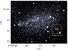 |
Fig. 1. Subaru Suprime-Cam Hα frame from Stonkutė et al. (2014, 2019). The H II region studied in this work is shown inside the yellow square and represents the VIMOS-IFU FoV. |
The paper is structured as follows. The VIMOS-IFU observations and data reduction are described in Section 2. The emission-line maps generated and metallicity estimates based on Te derivations are presented in Section 3. In Section 4, we explore possible ionisation mechanisms by comparing the distribution of young stars and the location of C2 with the H II region flux distributions. We also constrain the evolution of Leo A in the last 10 Gyr by using chemical evolution models. We present our conclusions in Section 5.
We adopted solar metallicities from Asplund et al. (2009), that is, the solar oxygen abundance of log(O/H)⊙ = 8.69 dex and the solar metallicity of Z⊙ = 0.0142.
2. Observations and data reduction
2.1. VIMOS observations and data reduction
Archival data correspond to a single gaseous nebula located in the south-west region of Leo A (α = 09h59m17.45s, δ = +30 ° 44′0.5″; J2000), as shown with the yellow square in Figure 1, representing the VIMOS-IFU field of view (FoV). This H II region has previously been identified as -101-052 (van Zee et al. 2006) and H II-west (Ruiz-Escobedo et al. 2018). Observations were obtained with the VIsible MultiObject Spectrograph (VIMOS, Le Fèvre et al. 2003) under the program 079.B-0877(A) in May 2007 (PI: M. Gullieuszik). VIMOS was a visible (360–1000 nm) wide-field imager and multi-object spectrograph mounted on Nasmyth focus B of VLT/UT 3 (Melipal). The integral-field-unit (IFU) mode was used. Two observing blocks (OBs) of one hour each were acquired.
The IFU comprises 1600 fibres (pseudo-slits), 400 of which are stored per quadrant. This provides a 27″ × 27″ FoV with a spatial resolution of 0.67″ px−1 in the wide-field mode, which is enough to cover the gaseous structure plus adjacent galaxy field free from nebular emission. Therefore, a significant number of fibres were used to generate the sky spectrum and perform decontamination by telluric lines. The selected spectral setup uses the HR-blue grism (4150−6200 Å, Δλ = 0.51 Å px−1, R = 2020). Emission lines with S/N > 3 were detected, including the Balmer emission lines Hβ and Hγ and the collisional excitation [O III]λλ 4959,5007 emission-line doublet.
Data cubes were reduced with the VIMOS Pipeline in the EsoReflex environment (Freudling et al. 2013), applying bias subtraction, flat normalisation, wavelength calibration, and flux calibration. The latter was based on spectrophotometric standard stars from Hamuy et al. (1992, 1994) and Moehler et al. (2014): the F-type LTT3864 (V = 12.17, B − V = 0.50), the G-type LTT7379 (V = 10.23, B − V = 0.61), and the DA-type EG247 (V = 11.03, B − V = −0.14). The final products are flux-calibrated in units of 10−16 erg s−1 cm−2 Å−1.
To reduce the noise in each spectral fibre, a smoothing technique was applied to each of them by weighting each bin by the mean of its three nearest neighbours. Finally, by fitting a second-order Chebyshev polynomial using the Specutils Python library (Astropy-Specutils Development Team 2019), we subtracted the continuum contribution.
2.2. Detection of the [O III]λ4363 emission line
We aim to estimate the electron temperature, Te, for two main reasons: (i) to characterise the physical properties of the H II region and (ii) to derive Te-based total oxygen abundances. Regarding the latter, we revisited the total oxygen abundance calculations on this H II region of VZ06 and R18, because the [O II]λ3727 emission-line flux measurement of the latter appears to be affected by spectral noise, potentially introducing instrumental biases into their O+/H+ determinations. VZ06, on the other hand, reported metallicities based on a spectrum with a well-detected [O II]λ3727 line, but their results rely on empirical and semi-empirical calibrations rather than direct Te measurements.
The procedure makes use of the auroral [O III]λ 4363 emission line (Peimbert 1967; Aller 1984). However, the integrated spectrum using all VIMOS-IFU fibres did not exhibit the auroral line with a signal-to-noise ratio (S/N) greater than 32. For this reason, we applied the Andrade et al. (2025) procedure to select the fibres that reproduce a detectable (S/N > 3) auroral line in the integrated spectra.
Since auroral and nebular transitions emerge from the same ionisation state (O++), their spatial distribution is expected to be similar. Therefore, we applied the ‘jump criterion’ to the [O III]λ5007 emission line. The jump is defined as the ratio between (i) the flux at the peak of the [O III]λ5007 emission line and (ii) the semi-quartile range of the spectral noise in the 4970−5040 Å interval. The semi-quartile range was chosen as it is less sensitive to outliers (i.e. emission lines are outliers with respect to the flux noise). By integrating all those fibres with jump = 1, the S/N of the auroral line was calculated. If the S/N is less than 3, we increased the jump threshold and repeated the iteration. At jump = 9, the integrated spectrum exhibits a clear [O III]λ4363 emission-line detection, as the result of combining 398 spectral fibres.
Figure 2 presents the integrated spectrum of the H II region. The flux scale is normalised by the flux at the peak of the Hβ line. The right panel shows the spatial distribution of the selected fibres, colour-coded by their jump values. The Hβ emission-line map is superimposed for reference with black contours. Most of the fibres producing the [O III]λ4363 detection were found in the zone with most ionisation, south-west of the nebula (see also Figure 3). Empty spaxels correspond to fibres lower than the jump threshold.
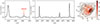 |
Fig. 2. Integrated VIMOS-IFU spectrum of the Leo A H II region normalised by the flux at the peak of the Hβ line. Left panel: spectral window showing Hγ and [O III]λ4363 detection, from left to right, respectively. Middle panel: spectral window presenting the Hβ, and the [O III]λλ 4959,5007 detection, from left to right, respectively. Right panel: spatial distribution of fibres selected to generate the integrated spectrum of the Leo H II region with [O III]λ4363 detection. The colour code represents the jump value of each selected fibre. The grey contours represent the Hβ emission of the nebula as a reference. |
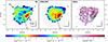 |
Fig. 3. Emission-line maps of the Leo A H II region. Left panel: Hβ emission-line map. Middle panel: [O III]λ5007 emission-line map. Right panel: Hβ/Hγ map, where the Hβ map contours are superimposed for reference. In all panels, the colour-code represents the flux of the emission lines per spectral fibre acquired by fitting Gaussian curves. The dashed grey lines are circles of increasing radius of 1.34″ (2 px) units up to 13.4″ (20 px). The dotted black lines show the angles that separate the south-western emission clump and the extended arc. |
To explore the chemical evolution of Leo A via gas-phase analysis, it is key to estimate its gas-phase Te-based oxygen abundance. However, the VIMOS spectral range does not include the [O II]λ3727 emission line, which prevents us from obtaining a direct estimate of O+/H+. To deal with this limitation, we reproduced the long-slit observations of van Zee et al. (2006, hereafter VZ06) and Ruiz-Escobedo et al. (2018, hereafter R18). This approach allowed us to (i) use their [O II]λ3727 fluxes to compute total oxygen abundances and (ii) to probe Te fluctuations across the nebula. The procedure is described in Appendix A.
Emission lines of the integrated spectrum of the H II region, as well as the VZ06 VIMOS and the R18 VIMOS mock slits, were fitted using single Gaussian curves with the Astropy Modelling library (Astropy Collaboration 2013). Fluxes were obtained by integrating the Gaussian curves with the Specutils library (Astropy-Specutils Development Team 2019), and uncertainties were derived from the covariance matrix of the fitting parameters.
Fluxes were corrected for dust attenuation via Balmer decrement. Assuming Case B recombination (Te ≃ 104 K and ne = 100 cm−3), we adopted the theoretical ratio IHβ/IHγ = 2.137 (Hummer & Storey 1987). The reddening constant was calculated as CHγ = [log(IHβ/IHγ)−log(FHβ/FHγ)]/[f(Hβ)−f(Hγ)], where f(λ) = ⟨A(λ)/A(V)⟩ is the extinction law at a given wavelength. The corrected fluxes were then obtained as Iλ/IHγ = (Fλ/FHγ)×10CHγ[f(λ)−f(Hγ)]. Following Cardelli et al. (1989), we adopted RV = 3.1. The dust-corrected emission-line fluxes, normalised to the Hγ flux, are reported for the integrated spectrum and the mock slits in Table 1.
Integrated emission-line flux measurements in the Leo A H II region, the VZ06 mock slit, and the R18 mock slit spectra.
3. Data analysis and results
3.1. Spatially resolved flux distributions
Figure 3 shows the Hβ (left panel) and [O III]λ5007 (middle panel) emission-line maps for the Leo A H II region. Line fluxes were measured in each fibre by integrating the Gaussian fits. Concentric circles with radii increasing in steps of 2 px (1.34″) up to 20 px (13.4″) are plotted for posterior analysis of radial flux profiles. To smooth out spatial variations and artefacts, the maps were smoothed using a bilinear interpolation. The centre of the nebula was defined as the position of the C2 star cluster candidate (Stonkutė et al. 2019).
The Hβ map (left panel) follows the Hα distribution observed with Subaru Suprime-Cam photometry Stonkutė et al. (2014, 2019), tracing a similar morphology to the Hβ emission (red curve in right panel of Figure 3; see also right panel of Figure 3 in Stonkutė et al. 2019), suggesting a uniform distribution. This is consistent with the Hβ/Hγ ratio map, which remains constant across the nebula. The morphology revealed was decomposed into an area of high emission towards the south-west and an extended arc with enhanced flux in the north-east.
The [O III]λ5007 map (middle panel) shows a distribution similar to that of ionised hydrogen, with significant emission in the centre. A prominent clump of ionisation is again observed in the south-west at the same location as that detected in the hydrogen map. This clump also exhibits a low Hβ/Hγ ratio (right panel), suggesting a low dust reddening in this region.
Radial flux-density profiles were constructed to characterise the structures identified in the emission-line maps, i.e., the south-western clump and the extended arc. The profiles are defined as Σλ = ∑Fλ/Aring, where ∑Fλ is the integrated flux within a ring of inner and outer radii, rin and rout, and angular range from ϕ0 to ϕf (counterclockwise in the x-axis). The ring area is
 (1)
(1)
For the arc component, we selected fibres with 40 ° < ϕ < 290°, while the south-west clump corresponds to 290 ° ≤ϕ < 360° and 0 ° ≤ϕ ≤ 40°. The angular selections are presented with the dotted black lines in the left and middle panels of Figure 3. The resulting flux-density profiles, expressed in units of 10−16 ergs s−1 cm−2 Å−1 arcsec−2, are shown in Figure 4.
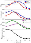 |
Fig. 4. Flux-density profiles for the south-western clump and the extended arc in red and blue, respectively. The top panel shows the radial Hβ flux-density profiles for both structures. The upper middle panel shows the radial [O III]λ5007 flux-density profile for both structures. The bottom middle panel shows the Hβ and [O III]λ5007 flux-density profile in purple and green, respectively, for the complete nebula integrated over the entire angular range. The bottom panel shows the Hβ/[O III]λ5007 ratio in black for the complete nebula integrated over the entire angular range. |
The upper panel of Figure 4 presents the Hβ profiles of the arc (blue) and the clump (red). Both components have comparable intensities, with the former peaking at ∼7″ and the latter at ∼5″. The [O III]λ5007 profiles (upper middle panel) show similar behaviour, where the arc peaks at ∼4″ and the clump peaks at ∼5″.
The bottom middle panel compares the Hβ and the [O III]λ5007 profiles for the entire H II region, i.e., integrating on the complete angular range (from 0° to 360°). The [O III]λ5007 emission is more centrally concentrated, while the Hβ dominates at larger radii. This behaviour is reinforced by the Hβ/[O III]λ5007 profile (bottom panel), which shows that [O III]λ5007 prevails over Hβ within ∼7″. Those features are a classical signature of ionized stratification; due to ionisation feedback (UV radiation from massive stars, stellar winds, and SNe explosions; Osterbrock & Ferland 2006) in a region containing young stellar objects, the surrounding ISM stores highly ionised species (such as O++ ), whereas the low-ionisation species prevail in the outskirts (such as H+, O+, N+, and S+), because the radiation decreases with distance.
These findings are similar to those observed in the SagDIG H II region (Andrade et al. 2025). A direct confirmation of stratification requires comparing O+ and O++ distributions using [O III]λ5007 and [O II]λ3727 emission lines, respectively. However, the VIMOS data do not cover wavelengths bluer than 4150 Å, and two-dimensional calibrated long-slit observations are not available for this nebula. Fortunately, indirect evidence is provided by the C2 star cluster candidate (age ∼20 Myr and M* ≥ 150 M⊙) detected by Stonkutė et al. (2019), based on HST/ACS and the Subaru Suprime-Cam photometry (see their Figure 3). This young stellar object is located at the centre of the nebula.
The ionised stratification in H II regions should have stellar systems responsible for bringing radiation to the ISM, so the location of C2 with the H+ and O++ distributions suggests that stellar feedback from this cluster is the primary source of ionisation and mechanical energy input, thus producing the stratified distribution. Moreover, if this is the case, the structure of the nebula may represent a classical bubble-like ionised-bound H II region (Pagel 1997; Osterbrock & Ferland 2006).
3.2. Electron temperature estimates
We estimated the gas-phase metallicity using the so-called direct method (Peimbert 1967; Aller 1984), which relies on electron temperature-sensitive lines together with the respective line emissivities. Electron temperatures were derived via nebular-to-auroral transitions of O++, i.e., [O III]λλ4959+5007/4363. Because the [O III]λ4363 line is typically two-to-three orders of magnitude fainter than Hβ (Maiolino & Mannucci 2019), it is often affected by spectral noise. The abundance determination also requires estimating the electron density, ne, which is generally obtained from [S II]λλ6717,6731. However, since our spectra do not extend beyond 6200 Å, we adopted ne = 100 cm−3 according to the low-density limit (Hummer & Storey 1987).
We computed Te[O III] using the nebular-to-auroral ratio with the getTemDen module of Pyneb (Luridiana et al. 2015). Then, the corresponding Te[O II] was obtained from the relation Te[O II] = 0.7 × Te[O III]+3000 given by Campbell et al. (1986).
For the integrated spectrum of the Leo A H II region, we derived Te[O III] = 22055 ± 2052 K. Using the mock slit fluxes, consistent results are obtained: Te[O III] = 22693 ± 426 K (VZ06 mock slit) and Te[O III] = 22332 ± 2047 K (R18 mock slit). Those values agree within the uncertainties, suggesting no significant temperature fluctuations across the nebula.
3.3. Te−based oxygen abundances
The total oxygen abundance is defined as 12 + log(O/H), where O/H = (O+/H+ + O++/H+). Because the VIMOS-IFU spectral range does not include [O II]λ3727, we reproduced the VZ06 and the R18 long-slit observations within our data cube to incorporate their [O II]λ3727 fluxes (see Appendix A). In addition, we also found discrepancies in the O+/H+ ionic abundance estimates, which come from VZ06 and R18 flux measurements, where the spectrum of the latter (their Figure 4) shows that [O II]λ3727 falls in the region with higher noise, likely affecting their flux measurements. This is not observed in the VZ06 spectrum (their Figure 2), where [O II]λ3727 is clearly detected. For this reason, and to provide an accurate measurement of the total Te-based oxygen abundance, we used the VZ06 [O II]λ3727 flux to derive O+/H+ and the VZ06 VIMOS mock slit to derive O++/H+. The detailed procedure, involving the combination and consistency checks, is described in Appendix B.
The Te-based metallicity is 12 + log(O/H) = 7.29 ± 0.06 dex (VZ06 mock slit). In addition, we also derived metallicities from the R23 strong-line index (Kobulnicky & Kewley 2004), returning 12 + log(O/H) = 7.44 ± 0.07 dex, in agreement with the empirical (∼7.48 dex) and the semi-empirical (7.44 ± 0.10 dex) estimates reported in VZ06.
In Section 3.2, we show that the three Te estimates (from both mock slits and the integrated spectrum) do not show significant Te fluctuations. However, they could be present as a thermal gradient (e.g. Andrade et al. 2025), but below the VIMOS-IFU sensitivity. Therefore, we took into account possible temperature fluctuations (Kobulnicky & Skillman 1996) in the abundance determination, which is a well-known systematic bias in when metallicities are derived using the Te−sensitive method (Peimbert 1967; Peimbert et al. 2017).
We applied the correction proposed by Cameron et al. (2023), which increases the abundance to 12 + log(O/H) = 7.46 ± 0.09. This correction should be taken with caution, as it was calibrated for higher metallicities and lower Te regimes. Despite this, the correction does not affect our interpretations regardless of whether the corrected or uncorrected abundance is adopted. The procedure of the Te corrections is described in Appendix C.
4. Discussion
4.1. Stellar distribution in the Leo A H II region
The stellar populations of Leo A have been extensively studied using HST/ACS and Subaru Suprime-Cam photometry (Cole et al. 2007; Stonkutė et al. 2014). The CMD reveals a well-defined red giant branch (RGB), red clump, and blue plume, together with a small population of asymptotic giant branch (AGB) stars (Cole et al. 2007; Stonkutė et al. 2014; Leščinskaitė et al. 2021; Leščinskaitė et al. 2022). This morphology reflects an extreme case of a ‘late-blooming’ SFH, such as the cases of Aquarius, WLM, and Leo P (Cole et al. 2014; McQuinn et al. 2024a,b); an initial episode more than 10 Gyr ago was followed by an ∼2 Gyr quiescent phase, after which the star formation was reignited and continued from ∼8 Gyr ago to the present day, peaking at rates five-to-ten times higher than the present. This SFH (Cole et al. 2007) is consistent with the behaviour of ‘slow dwarfs’ in the Gallart et al. (2015) framework and with the ‘two-component’ classification of Benítez-Llambay et al. (2015).
We related this stellar context to the properties of the Leo A H II region. For this purpose, we used the HST/ACS photometry3, which provides better spatial resolution compared with the Subaru data. This allows us to directly connect the location of the young stellar population with the ionised gas structure observed in the VIMOS-IFU cube.
To analyse the spatial distribution of stellar populations within the Leo A H II region, we applied a similar approach to that in Andrade et al. (2025). PARSEC v1.2S theoretical isochrones were fitted in the HST/ACS photometry, and colour cuts were used to classify stars into young MS and older populations (RGB and red clump stars), as described in Appendix D. The resulting classification is presented in Figure 5; young MS stars are shown with magenta triangles, old stars as cyan squares, and the full HST catalogue as grey points for reference.
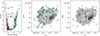 |
Fig. 5. Comparison of Leo A H II region with Hβ emission (grey contours) with HST/ACS photometry. The left panel shows the location of young MS stars (magenta triangles) and old stars (cyan squares). A 10 Myr PARSEC isochrone is shown with the black curve in order to obtain a proxy of the stellar masses of the young stars. The middle panel shows the spatial distribution of old stars in the H II region, whereas the right panel shows the distribution of young MS stars in the H II region. The most massive star is shown with the orange triangle, and those with masses of 8 < M⊙ < 10 are shown with green triangles. |
The middle and right panels of Figure 5 present the spatial distribution of these stellar populations relative to the Hβ emission (grey contours). The old stars are distributed uniformly across the H II region, but avoiding the south-west ionisation clump. In contrast, young MS stars are found all over the nebula, but with some preference for the centre and the ionisation clump.
To obtain a proxy of stellar masses, we compared the young MS population with a 10 Myr isochrone (grey curve in the left panel of Figure 5). Four stars consistent with masses of ∼8 − 10 M⊙ (green triangles) are located along the arc structure, while the most luminous star (yellow triangle), with an estimated mass of ∼15 M⊙ is found at the nebular centre.
4.2. Sources of ionisation in the Leo A H II region
Massive stars are the primary ionising sources of H II regions, through UV radiation, stellar winds, or via SN explosions (Osterbrock & Ferland 2006). Gull et al. (2022) reported tentative evidence that two out of four H II regions in Leo A (in the eastern sector) are powered by their central stars; these are labelled K1 and K2 with spectral types O9V and O9.7V, respectively. Their effective temperatures (Teff ∼ 30 900 and ∼31 600 K) and ages (∼10 and ∼8 Myr) produce photionisation production rates consistent with the approximations presented in nebular analyses (VZ06; R18).
The H II region analysed in this work was not included in Gull et al. (2022). Therefore, we investigated whether a single star or a clump of stars is ionising the H II region.
At the nebular centre of this H II region, the C2 star cluster candidate is located, identified by Stonkutė et al. (2019), with an age of ∼20 Myr and M ≥ 150 M⊙. We consider stars within 2.5″ (white symbols in the right panel of Figure 6) of the cluster centre as members of C2 (Stonkutė et al. 2019). The CMD analysis (left panel of Figure 6) shows that the brightest star (white cross) is consistent, with a mass of ∼15 M⊙ and an age of ∼10 Myr, while most of the surrounding stars (white squares and dots) have masses below 5 M⊙, suggested by the colour-code of the PARSEC isochrones. The isochrones predict Teff ∼ 33 200 K, which is comparable to K1 and K2 values reported by Gull et al. (2022), as also indicated by their location in the CMD (cyan triangle and diamond, respectively). This indicates that the most luminous star may be the dominating source of ionisation for the nebula.
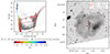 |
Fig. 6. Location of stars belonging to C2 star cluster (< 2.5″). Left panel: Location of stars in CMD. The white cross corresponds to the brightest star. The white squares are those stars with 23 < F814W < 24. Stars with F814W > 24 are shown as white dots. Theoretical PARSEC isochrones of 10 Myr, 100 Myr, 250 Myr, 500 Myr, 1 Gyr, and 5 Gyr are shown as colour-coded curves according to their stellar masses given by the theoretical isochrones. K1 and K2 O-type stars from Gull et al. (2022) are shown as the cyan triangle and the cyan diamond, respectively. Those massive stars are capable of ionising individually two Leo A H II regions. Right panel: Location of stars of the C2 star cluster in Leo A H II region (grey contours), superimposed with the HST/ACS F814W frame. |
To test this hypothesis, we estimated the stellar photoionisation produced rate, Q, using the PARSEC v2.0 evolutionary tracks (Nguyen et al. 2022; Costa et al. 2025). We took the mean Q value for stellar tracks between M ∈ [14, 16] M⊙, Z ∈ [0.006, 0.008], and Teff ∈ [30000, 35000] K, which results in Q = 1046.9 ± 0.17 photons s−1. Uncertainties were computed by taking the standard deviation of the Q values with the filters applied.
Then, an independent Q estimate was derived from nebular parameters. Assuming Case B recombination (Hummer & Storey 1987; Storey & Hummer 1995), the relation between Q and Hα luminosity is Q = 7.315 × 10¹¹L(Hα) (Kennicutt 1998; Choi et al. 2020). To estimate L(Hα), the theoretical relation I(Hα) = 2.86 I(Hβ) was used (Hummer & Storey 1987). We derive Q = 1047.17 ± 0.08 photons s−1. This value agrees within uncertainties with both the stellar estimate and the Hα-based determination of R18, Q = 1047.16 ± 0.01 photons s−1.
This consistency between the stellar and nebular Q estimates supports the conclusion that the central star of C2 is the main ionising source of this H II region. The Str mgren radius was estimated as follows:
 (2)
(2)
where ne is the electron density and αB(T) is the recombination coefficient at a given temperature. We adopted the empirical description of αB(T) from Lequeux (2005) using our measured Te, and under ne = 100 cm−3. This results in Rs = 3.2 ± 0.2 pc (red circle in Figure 6), consistent with the 2.7 pc derived by R18 from photoionisation models. However, the observed size of the nebula is ≃94 pc4 (R ≃ 47 pc), which is compatible with the physical scale of the Leo A galaxy presented in Leščinskaitė et al. (2022). Thus, the brightest star seems not to be enough to sustain ionisation of the complete H II region.
An estimate of ne as 131 ± 121 cm−3 is given by R18, using the [S II]λλ doublet, which is in line with the size-density relation of extragalactic H II regions of Hunt & Hirashita (2009). Hence, we relaxed the ne assumption. In this case, we derived Rs = 15 ± 1 pc (dashed red circle in Figure 6) under ne = 10 cm−3. This implies that the central star can only ionise ∼32% of the nebula. On the other hand, we find that at ne = 2 cm−3, Rs = 41 ± 3 pc is consistent with the radius of the H II region (dotted red circle in Figure 6).
The agreement between Q derived from stellar tracks and nebular parameters suggests that the star is indeed the dominant ionising source, similarly to the K1 and K2 stars powering other H II regions of Leo A (Gull et al. 2022) and analogous to the case of Leo P, where a single massive star sustains its only H II region with ionisation (Telford et al. 2023). However, depending on the adopted ne, the interpretations can change: if ne ≥ 10 cm−3, the star is not able to ionise the H II region completely, and additional ionising sources are required to explain the full size of the H II region, supported by the presence of the C2 star cluster. In this case the ionisation photon budget should be Q ≥ 1048.7 photons s−1 (Eq. (2)). On the contrary, if ne < 10 cm−3, the brightest star is able to completely ionise the H II region, which is supported by the fact that both Q estimates (that extracted by the stellar tracks, and that obtained with nebular parameters) agrees.
It is necessary to stress that these are rough approximations, since we assumed radial symmetry, uniform Te, and uniform ne distributions, which is not the case since emission-line maps (Figure 3) clearly show significant spatial variations.
4.3. The Leo A H II region in the mass-metallicity plane
The spatial analysis of the Leo A H II region with VIMOS-IFU, combined with HST/ACS photometry, suggests that the structure is strongly influenced by stellar feedback from the C2 cluster. The impact of stellar feedback can also be constrained by the chemical properties of the nebula.
VZ06 reported that the four H II regions of Leo A exhibit similar gas-phase metallicities (12 + log(O/H) ∼ 7.40) based on the empirical R23 calibrator. We therefore consider our Te-based total oxygen abundance for the nebula studied as representative of the galaxy as a whole. Adopting 3.3 ± 0.7 × 10⁶ M⊙ from Kirby et al. (2017), we consider both uncorrected and corrected metallicities for Te fluctations to place Leo A in the mass-metallicity plane, because most of the works that apply this method do not take into account this bias.
Figure 7 shows the position of Leo A in the mass-metallicity plane. The uncorrected and corrected values for Te fluctuations are shown as the white square and dot, respectively. On the other hand, the VZ06 R23-based abundance and the R18 Te-based abundance are shown with the red triangle and blue square, respectively. These are compared with the Te-based MZR of the local Universe of Andrews & Martini (2013) and Curti et al. (2020), as solid and dashed red curves, respectively. We also compared with the low-mass end of the MZRs of Lee et al. (2006) and Berg et al. (2012), as dashed and solid black lines, respectively. Our estimates place Leo A in agreement with the low-mass end of the MZR, within the 0.15 dex scatter of Lee et al. (2006).
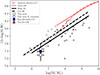 |
Fig. 7. Leo A in the mass-metallicity plane, with white square and white dot representing uncorrected and corrected metallicities for Te fluctuations, respectively. The VZ06 (R23) and R18 (Te−based) measures were included as the red triangle and blue square, respectively, for comparison. Dashed and solid black lines are the Lee et al. (2006) and the Berg et al. (2012) low-mass end of the MZR, respectively. The grey crosses and the grey dots are their respective samples. The solid red curve and the dashed red curve are the MZR of the local Universe from Andrews & Martini (2013) and Curti et al. (2020), respectively. |
The nature of the low-mass end of the MZR is still a matter of debate. Observations show that the scatter in the low-mass regime (Zahid et al. 2012) reflects the interplay of gas accretion, outflows, star formation, and environmental dependency, with the relative importance of those mechanisms varying on a galaxy-by-galaxy basis (e.g., Dalcanton et al. 2004; Petropoulou et al. 2012; Chisholm et al. 2018; Duarte Puertas et al. 2022). In theoretical frameworks, the picture is also diffuse, since the low-mass end of the MZR can be reproduced, for example, by (i) SNe driven winds (e.g. Finlator & Davé 2008; Davé et al. 2012; Guo et al. 2016), (ii) gas regulation by material flows plus star formation (Lilly et al. 2013), (iii) gas-infall-dominated galaxies where the star formation rate obeys the Kennicutt-Schimdt law subject to a gas density threshold (Tassis et al. 2008), and (iv) variations in the initial-mass function (IMF; Köppen et al. 2007).
4.4. Chemical evolution models of Leo A
Kirby et al. (2017, hereafter K17) used chemical-evolution models applied to the stellar metallicity distribution of Leo A, and suggested that the galaxy was either pre-enriched or acquired external gas during its SFH (K17, Figures 9 and 10). In addition, our results suggest that the ionised gas seems to be driven by stellar feedback. To test whether both perspectives are part of the same picture, we explored simple chemical-evolution models with a similar approach to that presented in Barrera-Ballesteros et al. (2018) and Olvera et al. (2024).
Old stars store the chemical composition of their natal clouds in their atmospheres. We therefore compared the present-day gas-phase metallicity of Leo A5,6 with the mean stellar metallicity7 of its old stellar population of ![Mathematical equation: $ {\langle} [\mathrm{Fe/H}] {\rangle} = -1.67^{+0.09}_{-0.08} $](/articles/aa/full_html/2026/03/aa55044-25/aa55044-25-eq5.gif) (Kirby et al. 2017).
(Kirby et al. 2017).
To properly apply the models, we also considered their stellar mass. Leo A has a present-day stellar mass of 3.3 ± 0.7 × 10⁶ M⊙ (Kirby et al. 2017),  of which was created 10 Gyr ago (z > 2), as estimated by Bermejo-Climent et al. (2018) by integrating the Leo A SFH.
We assumed that the mean stellar metallicity measured by K17 reflects the chemical state of Leo A 10 Gyr ago. This assumption is supported by observational evidence (K17, Figure 12) and by models of the age-metallicity relation (AMR), which remained flat from the beginning of star formation and up to ∼5 Gyr ago (Hidalgo 2017; Ruiz-Lara et al. 2018).
Analytic chemical-evolution models describe the gas-phase metallicity as Zg = Z(μ, y), which is a function of the gas fraction μ = Mgas/(M* + Mgas) and the yield y, defined as the mass fraction of metals produced by a stellar generation relative to the mass fraction locked up in stellar remnants and long-lived stars for a given IMF8 (Matteucci 2021). More realistic scenarios incorporate metal-poor inflows and metal-rich outflows.
We reproduced the evolution of the gas fraction with time. Today, Leo A has a gas mass of 6.9 ± 0.7 × 10⁶ M⊙ (Hunter et al. 2012) and a stellar mass of 3.3 ± 0.7 × 10⁶ M⊙ (K17), resulting in μ(t = 0) = 0.68 ± 0.05. On the other hand, 10 Gyr ago, adopting the same gas mass and the stellar mass 10 Gyr ago of Bermejo-Climent et al. (2018), the gas fraction was μ(t = 10 Gyr) = 0.92 ± 0.06. In both cases, the same gas mass was considered for consistency with the K17 results, i.e., the stellar populations are consistent with a pre-enriched closed-box or an accretion scenario for the evolution of Leo A.
We parametrised the evolution of the gas fraction with time with a linear interpolation, μ(t) = αt + μ(t = 0), with t ∈ [0, 10] Gyr and α as a free parameter. Therefore, the changes in the gas fraction with time track the build-up of stellar mass across cosmic time.
We tested four models of chemical evolution. The simplest is the so-called closed-box model (Searle & Sargent 1972), where a galaxy is treated as a system with no material flows into or out of the galaxy. The chemical enrichment is driven only by star formation. In this framework, part of the gas expelled by SNe explosions is used to form new generations of stars, and the remaining gas is used to enrich the ISM. The gas metallicity evolves as
 (3)
(3)
where y is the yield and μ is the gas fraction. Under this approximation, the metallicity asymptotically approaches to Zg = y at the end of the SFH of a system.
The second is the accretion model (Larson 1972; Tinsley 1980), which includes continuous infall of metal-poor gas. The metallicity is as follows:
![Mathematical equation: $$ \begin{aligned} Z_{g} = y_{\mathrm{eff} } \left[ 1- e^{\left(1-\mu ^{-1}\right)} \right] ,\end{aligned} $$](/articles/aa/full_html/2026/03/aa55044-25/aa55044-25-eq8.gif) (4)
(4)
where yeff is known as the effective yield, which is lower than the true yield of the closed-box model. In this scenario, and the next model introduced, yeff represents the highest degree of chemical enrichment for a given IMF (Matteucci 2021).
The third case is the leaky-box model (Matteucci & Chiosi 1983), for a galaxy suffering mass loss through outflows. The metallicity is given by
![Mathematical equation: $$ \begin{aligned} Z_{g} = \frac{y_{\mathrm{eff} }}{1+\lambda } \ \ln {\left[ (1+\lambda )\mu ^{-1} - \lambda \right]}, \end{aligned} $$](/articles/aa/full_html/2026/03/aa55044-25/aa55044-25-eq9.gif) (5)
(5)
where λ is the mass-loading factor and quantifies the amount of gas expelled from the galaxy relative to star formation.
Finally, we considered the gas-regulator or ‘bathtub’ model of Lilly et al. (2013). Here, the global SFR across cosmic time is regulated by variations of the gas reservoir subject to inflows, outflows, gas used to form long-lived stars, and instantaneous recycling to enrich the ISM. The metallicity is expressed as
 (6)
(6)
where rgas = μ/(1 − μ) is the gas-to-stellar mass ratio, 1 − R is the amount of gas used to create long-lived stars, and ϵ is the star formation efficiency. Following Lilly et al. (2013) and Barrera-Ballesteros et al. (2018), we used R = 0.4 and  .
.
To apply these solutions, we evolved the gas fraction between 10 Gyr ago and the present day using the linear interpolation described above. For each model, we ran Monte Carlo simulations, sampling μ(t = 0) and μ(t = 10) from Gaussian distributions centred on their estimated value with σ settled by their uncertainties. For the closed-box and accretion models, we ran 1000 simulations per yeff from 0.001 to 0.02 (steps of 0.001). For the leaky-box and the gas-regulator models, we ran 1000 simulations over the same yeff combined with λ values from 0 to 35 (steps of 1).
Figure 8 compares the chemical state of Leo A at the present day and 10 Gyr ago. The present-day gas-phase abundances, with Te correction and without correction, are shown as the white dot (left panel) and white triangle (right panel), together with the stellar metallicity (white squares in both panels, representing the chemical status of Leo A 10 Gyr ago).
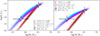 |
Fig. 8. Evolution of Leo A over the last 10 Gyr in the mass-metallicity plane. Left panel: White square represents Leo A 10 Gyr ago, whereas the white dot represents Leo A in the present day. The closed-box-model and accretion-model median tracks that approach our estimates are shown as the dotted black and dashed red lines, respectively. The leaky-box and the gas-regulator (bathtub) model median tracks that reproduce our estimates are shown with the solid magenta and the dashed cyan curves, respectively. The closed-box, accretion, leaky-box, and gas-regulator tracks generated by the Monte Carlo simulations are shown with the semi-transparent black, red, magenta, and cyan curves, respectively. Right panel: Same as left panel, but using the Te− corrected gas-phase metallicity as the present-day chemical status of Leo A, shown with the white triangle. |
When using the Te corrected gas-phase metallicity (left panel), the closed-box (dotted black) and accretion models (dashed red) require yeff = 0.0022 ± 0.0005 to match the present-day abundance. However, these scenarios fail to reproduce the full chemical evolution of Leo A, as their mean evolutionary tracks are not consistent with the stellar and gas-phase metallicity constraints. On the other hand, the leaky-box model (dashed magenta) with yeff = 0.005 ± 0.001 and λ = 10, and the gas-regulator model (dotted cyan) with yeff = 0.005 ± 0.001 and λ = 5, produce tracks that successfully connect the chemical status of Leo A 10 Gyr ago and at the present day, in the mass-metallicity plane. The Monte Carlo simulations are shown with their respective colours as semi-transparent curves.
When using the non-Te-corrected gas-phase abundance (red panel), the results are similar: closed-box and accretion scenarios fail to reproduce the Leo A chemical evolution, while the leaky-box (yeff = 0.007 ± 0.002, λ ∼ 32) and accretion models (yeff = 0.006 ± 0.002, λ ∼ 12) successfully reproduce the estimated evolution. In both Te-corrected and uncorrected cases, the key parameter is the inclusion of mass loss.
In the mass-metallicity plane, closed-box and accretion models behave similarly. The same is observed with the leaky-box and gas-regulator models. Those features comes from the functional form in the solutions of the four models. The detailed procedure exploring these features is presented in Appendix E.
Previous works such as Garnett (2002) have suggested yeff ≃ 0.002 in the closed-box framework, while K17 derived yeff ≃ 0.005 under a pre-enriched or accretion scenario. Our calculations closely agree with the latter and are consistent with yeff of dwarf galaxies in the Local Universe with comparable masses (Garnett 2002; Tortora et al. 2022).
Leaky-box and gas-regulator models indicate that outflows must be considered in the evolution of Leo A. The mass-loading factor that reproduces the chemical evolution of Leo A differs between them. This difference lies in their main assumptions: the leaky box describes a closed box with outflows, while the gas regulator incorporates the balance of inflows, outflows, and star formation, regulating the gas reservoir.
Based on the fact that the Leo A evolution is being described by a leaky-box model, the simplest interpretation is that Leo A is driven by galaxy-scale outflows. However, the evolution of gas fractions was constructed under constant accretion, as K17 suggests. Therefore, our leaky-box model is an accretion model with material loss driven by stellar feedback. In other words, our leaky-box model is a rough approximation of the gas-regulator model, explaining why both reproduce the observed evolution with similar tracks but different values of λ.
Our interpretation is therefore that Leo A was either pre-enriched or acquired significant gas during its early star formation, allowing for the development of its stellar metallicity distribution. Today, however, stellar feedback and gas loss play a significant role. The present-day evolution of Leo A appears to be governed by a balance between gas flows and star formation, i.e. a gas-equilibrium framework (e.g. Finlator & Davé 2008; Tortora et al. 2022) under a roughly constant yeff from 10 Gyr to the present day. In this context, the conclusions of K17 and our results are complementary, providing a coherent picture of the chemical evolution of Leo A across cosmic time.
5. Summary and conclusions
We analysed intermediate-resolution optical VIMOS-IFU/VLT archival data of one of the four H II regions in Leo A. We explored the nebular morphology through emission-line maps. We derived Te-based total oxygen abundances, and we used HST photometry to link young stellar populations with the gaseous structure and tested chemical-evolution models of Leo A over the past 10 Gyr.
Our main conclusions can be summarised as follows:
-
The Hβ map shows weak central emission, whereas [O III]λ5007 remains strong at the centre, indicating ionised stratification, with O++ more centrally concentrated than H+.
-
The young MS stars found in the nebular centre of the H II region correspond to the C2 star cluster identified by Stonkutė et al. (2019).
-
The brightest MS star, located in the nebular centre, seems to be an O-type star with ∼15 M⊙ and Teff ∼ 33 200 K.
-
By extracting mock slits following VZ06 and R18, we measured Te = 22 693 ± 436 K for the H II region. The Te-based derived metallicity is 12 + log(O/H) = 7.29 ± 0.06 dex, while the R23-based derived metallicity is 12 + log(O/H) = 7.45 ± 0.07, in agreement with the empirical and semi-empirical values reported by VZ06.
-
Applying the Cameron et al. (2023) calibration to correct for Te fluctuations, we derived Te = 16431 ± 1203 and a metallicity of 12 + log(O/H) = 7.45 ± 0.09, which is ∼0.16 dex higher than the uncorrected value.
-
The leaky-box and gas-regulator models reproduce the stellar-mass growth (∼2.4 × 10⁶ M⊙) and chemical enrichment (∼0.4 dex) over the last 10 Gyr with yeff ∼ 0.005 ± 0.001, consistent with K17, a value slightly larger than the closed-box approximation presented in previous works (Garnett 2002), but in line with estimates of other dwarf galaxies in the Local Universe (Garnett 2002; Tortora et al. 2022). This points to a scenario where Leo A experienced significant gas accretion, while stellar feedback and mass loss regulate its present-day chemical evolution.
Acknowledgments
We thank the anonymous referee for their useful and professional comments which improved the quality of the paper. L. M. and A. A. acknowledge support from ANID-FONDECYT Regular Project 1251809.
References
- Aller, L. H. 1984, Astrophysics and Space Science Library (Dordrecht: Reidel) [Google Scholar]
- Andrade, A., Saviane, I., Monaco, L., et al. 2025, A&A, 699, A281 [NASA ADS] [CrossRef] [EDP Sciences] [Google Scholar]
- Andrews, B. H., & Martini, P. 2013, ApJ, 765, 140 [NASA ADS] [CrossRef] [Google Scholar]
- Asplund, M., Grevesse, N., Sauval, A. J., et al. 2009, ARA&A, 47, 481 [Google Scholar]
- Astropy Collaboration (Robitaille, T. P., et al.) 2013, A&A, 558, A33 [NASA ADS] [CrossRef] [EDP Sciences] [Google Scholar]
- Astropy-Specutils Development Team. 2019, Astrophysics Source Code Library [record ascl:1902.012] [Google Scholar]
- Barman, S., Neelamkodan, N., Madden, S. C., et al. 2022, ApJ, 930, 100 [NASA ADS] [CrossRef] [Google Scholar]
- Barrera-Ballesteros, J. K., Heckman, T., Sánchez, S. F., et al. 2018, ApJ, 852, 74 [Google Scholar]
- Benítez-Llambay, A., Navarro, J. F., Abadi, M. G., et al. 2015, MNRAS, 450, 4207 [CrossRef] [Google Scholar]
- Berg, D. A., Skillman, E. D., Marble, A. R., et al. 2012, ApJ, 754, 98 [NASA ADS] [CrossRef] [Google Scholar]
- Bermejo-Climent, J. R., Battaglia, G., Gallart, C., et al. 2018, MNRAS, 479, 1514 [NASA ADS] [CrossRef] [Google Scholar]
- Bernard, E. J., Monelli, M., Gallart, C., et al. 2009, ApJ, 699, 1742 [NASA ADS] [CrossRef] [Google Scholar]
- Bernard, E. J., Monelli, M., Gallart, C., et al. 2013, MNRAS, 432, 3047 [Google Scholar]
- Bressan, A., Marigo, P., Girardi, L., et al. 2012, MNRAS, 427, 127 [NASA ADS] [CrossRef] [Google Scholar]
- Cameron, A. J., Katz, H., & Rey, M. P. 2023, MNRAS, 522, L89 [NASA ADS] [CrossRef] [Google Scholar]
- Campbell, A., Terlevich, R., & Melnick, J. 1986, MNRAS, 223, 811 [NASA ADS] [CrossRef] [Google Scholar]
- Cardelli, J. A., Clayton, G. C., & Mathis, J. S. 1989, ApJ, 345, 245 [Google Scholar]
- Chisholm, J., Tremonti, C., & Leitherer, C. 2018, MNRAS, 481, 1690 [NASA ADS] [CrossRef] [Google Scholar]
- Choi, S. K., Hasselfield, M., Ho, S.-P. P., et al. 2020, JCAP, 2020, 045 [CrossRef] [Google Scholar]
- Cole, A. A., Skillman, E. D., Tolstoy, E., et al. 2007, ApJ, 659, L17 [Google Scholar]
- Cole, A. A., Weisz, D. R., Dolphin, A. E., et al. 2014, ApJ, 795, 54 [Google Scholar]
- Costa, G., Shepherd, K. G., Bressan, A., et al. 2025, A&A, 694, A193 [NASA ADS] [CrossRef] [EDP Sciences] [Google Scholar]
- Curti, M., Mannucci, F., Cresci, G., et al. 2020, MNRAS, 491, 944 [NASA ADS] [CrossRef] [Google Scholar]
- Dalcanton, J. J., Yoachim, P., & Bernstein, R. A. 2004, ApJ, 608, 189 [NASA ADS] [CrossRef] [Google Scholar]
- Davé, R., Finlator, K., & Oppenheimer, B. D. 2012, MNRAS, 421, 98 [Google Scholar]
- Dolphin, A. E., Saha, A., Claver, J., et al. 2002, AJ, 123, 3154 [Google Scholar]
- Duarte Puertas, S., Vilchez, J. M., Iglesias-Páramo, J., et al. 2022, A&A, 666, A186 [NASA ADS] [CrossRef] [EDP Sciences] [Google Scholar]
- Emsellem, E., Schinnerer, E., Santoro, F., et al. 2022, A&A, 659, A191 [NASA ADS] [CrossRef] [EDP Sciences] [Google Scholar]
- Esteban, C., García-Rojas, J., Carigi, L., et al. 2014, MNRAS, 443, 624 [NASA ADS] [CrossRef] [Google Scholar]
- Finlator, K., & Davé, R. 2008, MNRAS, 385, 2181 [NASA ADS] [CrossRef] [Google Scholar]
- Freudling, W., Romaniello, M., Bramich, D. M., et al. 2013, A&A, 559, A96 [NASA ADS] [CrossRef] [EDP Sciences] [Google Scholar]
- Gallart, C., Monelli, M., Mayer, L., et al. 2015, ApJ, 811, L18 [NASA ADS] [CrossRef] [Google Scholar]
- Garnett, D. R. 2002, ApJ, 581, 1019 [NASA ADS] [CrossRef] [Google Scholar]
- Gull, M., Weisz, D. R., Senchyna, P., et al. 2022, ApJ, 941, 206 [NASA ADS] [CrossRef] [Google Scholar]
- Guo, Y., Koo, D. C., Lu, Y., et al. 2016, ApJ, 822, 103 [NASA ADS] [CrossRef] [Google Scholar]
- Hamuy, M., Walker, A. R., Suntzeff, N. B., et al. 1992, PASP, 104, 533 [NASA ADS] [CrossRef] [Google Scholar]
- Hamuy, M., Suntzeff, N. B., Heathcote, S. R., et al. 1994, PASP, 106, 566 [NASA ADS] [CrossRef] [Google Scholar]
- Hidalgo, S. L. 2017, A&A, 606, A115 [NASA ADS] [CrossRef] [EDP Sciences] [Google Scholar]
- Hummer, D. G., & Storey, P. J. 1987, MNRAS, 224, 801 [NASA ADS] [CrossRef] [Google Scholar]
- Hunt, L. K., & Hirashita, H. 2009, A&A, 507, 1327 [NASA ADS] [CrossRef] [EDP Sciences] [Google Scholar]
- Hunter, D. A., Ficut-Vicas, D., Ashley, T., et al. 2012, AJ, 144, 134 [CrossRef] [Google Scholar]
- Izotov, Y. I., & Thuan, T. X. 2004, ApJ, 602, 200 [CrossRef] [Google Scholar]
- James, B. L., Tsamis, Y. G., & Barlow, M. J. 2010, MNRAS, 401, 759 [NASA ADS] [CrossRef] [Google Scholar]
- James, B. L., Tsamis, Y. G., Barlow, M. J., et al. 2013, MNRAS, 428, 86 [NASA ADS] [CrossRef] [Google Scholar]
- James, B. L., Kumari, N., Emerick, A., et al. 2020, MNRAS, 495, 2564 [NASA ADS] [CrossRef] [Google Scholar]
- Katz, H. 2022, MNRAS, 512, 348 [NASA ADS] [CrossRef] [Google Scholar]
- Kennicutt, R. C. 1998, ARA&A, 36, 189 [NASA ADS] [CrossRef] [Google Scholar]
- Kirby, E. N., Rizzi, L., Held, E. V., et al. 2017, ApJ, 834, 9 [Google Scholar]
- Kobulnicky, H. A., & Kewley, L. J. 2004, ApJ, 617, 240 [CrossRef] [Google Scholar]
- Kobulnicky, H. A., & Skillman, E. D. 1996, ApJ, 471, 211 [NASA ADS] [CrossRef] [Google Scholar]
- Köppen, J., Weidner, C., & Kroupa, P. 2007, MNRAS, 375, 673 [CrossRef] [Google Scholar]
- Kreckel, K., Egorov, O. V., Egorova, E., et al. 2024, A&A, 689, A352 [NASA ADS] [CrossRef] [EDP Sciences] [Google Scholar]
- Kumari, N., James, B. L., & Irwin, M. J. 2017, MNRAS, 470, 4618 [NASA ADS] [CrossRef] [Google Scholar]
- Kumari, N., James, B. L., Irwin, M. J., et al. 2018, MNRAS, 476, 3793 [NASA ADS] [CrossRef] [Google Scholar]
- Larson, R. B. 1972, Nat. Phys. Sci., 236, 7 [NASA ADS] [CrossRef] [Google Scholar]
- Le Fèvre, O., Saisse, M., Mancini, D., et al. 2003, Proc. SPIE, 4841, 1670 [NASA ADS] [CrossRef] [Google Scholar]
- Lee, H., Skillman, E. D., & Venn, K. A. 2005, ApJ, 620, 223 [Google Scholar]
- Lee, H., Skillman, E. D., Cannon, J. M., et al. 2006, ApJ, 647, 970 [NASA ADS] [CrossRef] [Google Scholar]
- Lequeux, J. 2005, in The Interstellar Medium, (Berlin: Springer), Astronomy and Astrophysics Library [Google Scholar]
- Leščinskaitė, A., Stonkutė, R., & Vansevičius, V. 2021, A&A, 647, A170 [CrossRef] [EDP Sciences] [Google Scholar]
- Leščinskaitė, A., Stonkutė, R., & Vansevičius, V. 2022, A&A, 660, A79 [NASA ADS] [CrossRef] [EDP Sciences] [Google Scholar]
- Lilly, S. J., Carollo, C. M., Pipino, A., et al. 2013, ApJ, 772, 119 [NASA ADS] [CrossRef] [Google Scholar]
- Luridiana, V., Morisset, C., & Shaw, R. A. 2015, A&A, 573, A42 [NASA ADS] [CrossRef] [EDP Sciences] [Google Scholar]
- Maiolino, R., & Mannucci, F. 2019, A&ARv, 27, 3 [Google Scholar]
- Matteucci, F. 2021, A&ARv, 29, 5 [NASA ADS] [CrossRef] [Google Scholar]
- Matteucci, F., & Chiosi, C. 1983, A&A, 123, 121 [NASA ADS] [Google Scholar]
- McConnachie, A. W. 2012, AJ, 144, 4 [Google Scholar]
- McQuinn, K. B. W., Newman, M. J. B., Savino, A., et al. 2024a, ApJ, 961, 16 [Google Scholar]
- McQuinn, K. B. W., Newman, M. J. B., Skillman, E. D., et al. 2024b, ApJ, 976, 60 [Google Scholar]
- Méndez-Delgado, J. E., Esteban, C., García-Rojas, J., et al. 2023a, Nature, 618, 249 [Google Scholar]
- Méndez-Delgado, J. E., Esteban, C., García-Rojas, J., et al. 2023b, MNRAS, 523, 2952 [CrossRef] [Google Scholar]
- Moehler, S., Modigliani, A., Freudling, W., et al. 2014, A&A, 568, A9 [NASA ADS] [CrossRef] [EDP Sciences] [Google Scholar]
- Monelli, M., Gallart, C., Hidalgo, S. L., et al. 2010, ApJ, 722, 1864 [NASA ADS] [CrossRef] [Google Scholar]
- Nguyen, C. T., Costa, G., Girardi, L., et al. 2022, A&A, 665, A126 [NASA ADS] [CrossRef] [EDP Sciences] [Google Scholar]
- Olvera, A. J., Borthakur, S., Padave, M., et al. 2024, ApJ, 976, 205 [Google Scholar]
- Osterbrock, D. E., & Ferland, G. J. 2006, Astrophysics of Gaseous Nebulae and Active Galactic Nuclei, 2nd edn. (Sausalito, CA: University Science Books) [Google Scholar]
- Pagel, B. E. J. 1997, Nucleosynthesis and Chemical Evolution of Galaxies (Cambridge, UK: Cambridge University Press), 392 [Google Scholar]
- Peimbert, M. 1967, ApJ, 150, 825 [NASA ADS] [CrossRef] [Google Scholar]
- Peimbert, M., Peimbert, A., & Delgado-Inglada, G. 2017, PASP, 129, 082001 [NASA ADS] [CrossRef] [Google Scholar]
- Pérez-Montero, E., Vílchez, J. M., Cedrés, B., et al. 2011, A&A, 532, A141 [CrossRef] [EDP Sciences] [Google Scholar]
- Petropoulou, V., Vílchez, J., & Iglesias-Páramo, J. 2012, ApJ, 749, 133 [NASA ADS] [CrossRef] [Google Scholar]
- Pilyugin, L. S., & Grebel, E. K. 2016, MNRAS, 457, 3678 [NASA ADS] [CrossRef] [Google Scholar]
- Press, W. H., & Schechter, P. 1974, ApJ, 187, 425 [Google Scholar]
- Ruiz-Escobedo, F., Peña, M., Hernández-Martínez, L., et al. 2018, MNRAS, 481, 396 [Google Scholar]
- Ruiz-Lara, T., Gallart, C., Beasley, M., et al. 2018, A&A, 617, A18 [NASA ADS] [CrossRef] [EDP Sciences] [Google Scholar]
- Sánchez, S. F. 2013, Adv. Astron., 2013, 1 [CrossRef] [Google Scholar]
- Sánchez-Janssen, R., Amorín, R., García-Vargas, M., et al. 2013, A&A, 554, A20 [NASA ADS] [CrossRef] [EDP Sciences] [Google Scholar]
- Saviane, I., Rizzi, L., Held, E. V., et al. 2002, A&A, 390, 59 [NASA ADS] [CrossRef] [EDP Sciences] [Google Scholar]
- Saviane, I., Ivanov, V. D., Held, E. V., et al. 2008, A&A, 487, 901 [NASA ADS] [CrossRef] [EDP Sciences] [Google Scholar]
- Schechter, P. 1976, ApJ, 203, 297 [Google Scholar]
- Searle, L., & Sargent, W. L. W. 1972, ApJ, 173, 25 [NASA ADS] [CrossRef] [Google Scholar]
- Skillman, E. D., Salzer, J. J., Berg, D. A., et al. 2013, AJ, 146, 3 [CrossRef] [Google Scholar]
- Stonkutė, R., Arimoto, N., Hasegawa, T., et al. 2014, ApJS, 214, 19 [Google Scholar]
- Stonkutė, R., Naujalis, R., Čeponis, M., et al. 2019, A&A, 627, A7 [NASA ADS] [CrossRef] [EDP Sciences] [Google Scholar]
- Storey, P. J., & Hummer, D. G. 1995, MNRAS, 272, 41 [NASA ADS] [CrossRef] [Google Scholar]
- Tassis, K., Kravtsov, A. V., & Gnedin, N. Y. 2008, ApJ, 672, 888 [NASA ADS] [CrossRef] [Google Scholar]
- Telford, O. G., McQuinn, K. B. W., Chisholm, J., et al. 2023, ApJ, 943, 65 [NASA ADS] [CrossRef] [Google Scholar]
- Tinsley, B. M. 1980, Fund. Cosmic Phys., 5, 287 [Google Scholar]
- Tolstoy, E., Hill, V., & Tosi, M. 2009, ARA&A, 47, 371 [Google Scholar]
- Tortora, C., Hunt, L. K., & Ginolfi, M. 2022, A&A, 657, A19 [NASA ADS] [CrossRef] [EDP Sciences] [Google Scholar]
- Tremonti, C. A., Heckman, T. M., Kauffmann, G., et al. 2004, ApJ, 613, 898 [Google Scholar]
- Urbaneja, M. A., Bresolin, F., & Kudritzki, R.-P. 2023, ApJ, 959, 52 [Google Scholar]
- van Zee, L., Skillman, E. D., & Haynes, M. P. 2006, ApJ, 637, 269 [Google Scholar]
- Vanzi, L., Cresci, G., Sauvage, M., et al. 2011, A&A, 534, A70 [NASA ADS] [CrossRef] [EDP Sciences] [Google Scholar]
- Weisz, D. R., Dalcanton, J. J., Williams, B. F., et al. 2011, ApJ, 739, 5 [CrossRef] [Google Scholar]
- Weisz, D. R., Dolphin, A. E., Skillman, E. D., et al. 2014, ApJ, 789, 147 [Google Scholar]
- Weisz, D. R., McQuinn, K. B. W., Savino, A., et al. 2023, ApJS, 268, 15 [Google Scholar]
- Zahid, H. J., Bresolin, F., Kewley, L. J., et al. 2012, ApJ, 750, 120 [CrossRef] [Google Scholar]
The yield (yi) is defined as the mass fraction of an element, i, produced by a generation of stars relative to the fraction of mass locked up in stellar remnants and long-lived stars (Matteucci 2021).
We define signal (S) as the flux value at the peak of the evaluated emission line and noise (N) as the standard deviation evaluated on both sides of the line inside a spectral window of 5 px per region.
Based on measuring the pixel length along the south-east to north-west diagonal (36 px) in the Hβ emission line map, generated by selecting all fibers where Hβ and [O III]λ5007 have a S/N > 3. We adopted the Leo A distance of 800 kpc (Dolphin et al. 2002).
log(Z/Z⊙) = 12 + log(O/H)−8.69 = −1.39 ± 0.06.
log(Z/Z⊙) = 12 + log(O/H)Te − corrected − 8.69 = −1.23 ± 0.09.
log(Z/Z⊙) = [Fe/H]+0.75[α/Fe] = −1.65 ± 0.09 (Kirby et al. 2017).
The yield, y, is described as  , where pm is the yield of metals per stellar mass, ϕ(m) is the IMF, and R is the returned fraction, as the fraction of mass ejected into the ISM by a entire stellar generation (Tinsley 1980).
Appendix A: Mock slits in the VIMOS-IFU data cube
The Te-based total oxygen abundances require the [O II]λ3727 emission line, which lies outside the VIMOS-IFU spectral range. Consequently, it is not possible to derive directly O+/H+ from our data. To deal with this limitation, we simulated the slit positions and orientations of the long-slit observations of VZ06 and R18, allowing us to combine their [O II]λ3727 fluxes with our IFU results to compute total oxygen abundances.
VZ06 observed the H II region, labelled −101 − 052, with a 2″ wide slit centred at α = 9h59m17.2s and δ = +30 ° 44′07″ (J2000), and position angle of 73°. On the other hand, R18 employed a 7.4′ long and 1.8″ wide slit to cover two H II regions of Leo A: the western H II region studied here (H II-west) and an eastern H II region at α = 9h59m24.5s; δ = 30 ° 44′59″ (J2000; see R18, Figure 1).
The slit positions are shown in Figure A.1, where the yellow square presents the VIMOS-IFU FOV (covering H II-west). The cyan line shows the R18 slit, and the red line the VZ06 slit. The red cross marks the location of H II-east. A slight inclination difference between the two slit orientations is observed.
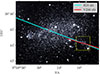 |
Fig. A.1. Subaru Suprime-Cam Hα frame from Stonkutė et al. (2014, 2019). The yellow square is the VIMOS-IFU FOV. The cyan line represents the R18 slit position, which goes from H II west (yellow square), to the H II east (red cross). The red line represents the VZ06 slit position. |
Since the VIMOS spatial scale is 0.67″ px−1, we reproduced both slits as extractions of 3 px (2.01″) width on the IFU cube. The resulting integrated spectra are presented in Figure A.2, showing the VZ06 mock slit in red and the R18 mock slit in blue (left and middle panels). The right panel shows the position of the mock slits over the Hβ emission line map for reference (black contours). Both mock-slit spectra exhibit a detectable [O III]λ4363 emission line, and present in general similar emission line fluxes with slight differences. The corresponding flux measurements and dust-corrected intensities are listed in Table 1 of Section 2.2.
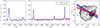 |
Fig. A.2. Integrated spectrum of the Leo A H II region using the VZ06 and R18 mock slits, with red and blue colours, respectively. Left panel: spectral window showing Hγ and [O III]λ4363 detection, from left to right, respectively. Middle panel: spectral window presenting the Hβ, and the [O III]λλ 4959,5007 detection, from left to right, respectively. Right panel: spatial distribution of pixels selected to reproduce both mock slits in the H II region. The grey contours represent the Hβ emission of the nebula for reference. |
Appendix B: Combination of long-slit and the VIMOS-IFU mock-slit spectrum for Te−based metallicity estimations
As mentioned in the main text, the [O II]λ3727 emission line is outside the VIMOS-IFU spectral range, so only O++/H+ can be measured directly. To derive total oxygen abundances, we therefore combined [O II]λ3727 fluxes to obtain O+/H+ from the long-slit spectra of VZ06 and R18 with O++/H+ estimates from our VIMOS mock slits.
B.1. Procedure
We estimated total oxygen abundances as follows:
-
(i): Extract [O II]λ3727 and Hβ from VZ06, Table 3 to obtain O+/H+.
-
(ii): Compare O++/H+ derived from the VZ06 mock slit with that obtained using VZ06, Table 3 fluxes.
-
(iii): Combine O+/H+ and O++/H+ to compute Te-based metallicity.
-
(iv): Use [O II]λ3727 over Hβ from VZ06, Table 3 to combine with [O III]λ4959 +[O III]λ5007 over Hβ from their mock slit to compute R23-based metallicities. Then, compare with R23 metallicities using VZ06 fluxes only.
-
(v) Repeat (i), (ii), (iii), and (iv) with R18, Table 3 fluxes and the R18 mock slit.
To ensure consistency, we applied our dust correction to the raw VZ06 fluxes, since their correction assume Case B recombination with Hγ/Hβ = 0.474 at Te = 15000 K, and ne = 100 cm−3, whereas we adopt Hγ/Hβ = 0.468 at Te = 10000 K, and ne = 100 cm−3.
B.2. Combination of ionic abundances
Total oxygen abundances were obtained by combining O+/H+ from VZ06 and R18 with O++/H+ from the VIMOS mock slits, as follows
 (B.1)
(B.1)
For comparison, abundances were also derived using only the long-slit data, under Te derived from the VIMOS mock slits:
 (B.2)
(B.2)
The reliability of the combination will be observed as consistency within the uncertainties between both equations, as well as the ionic O++/H+ abundances from the VIMOS mock slits and the ones derived from the long-slit datasets of VZ06 and R18.
Temperatures were combined with getTemDen Pyneb module from the [O III]λλ4959,5007 / λ4363 ratio, and Te[O II] from the relation of Campbell et al. (1986). Ionic abundances were obtained with the getIonAbundance Pyneb module.
B.3. Results and discrepancies
The values derived are listed in Table B.1. VZ06 and its VIMOS mock slit are in agreement, returning 12 + log(O/H)≃7.29 dex. R18 and their VIMOS mock slit are also in agreement within uncertainties, as 7.38 ± 0.05 and 7.40 ± 0.10, respectively. However, those are systematically higher than VZ06 by ∼0.1 dex, despite their similar Te values (∼22300 K).
Electron temperatures, ionic and total oxygen abundances estimates for the Leo A H II region.
Further exploration led to an analysis of ionic oxygen abundances. We found that the offset comes from O+/H+ estimates. The R18 O+/H+ estimates are higher by ∼0.15 dex. This may come from an inaccurate [O II]λ3727 emission line estimation, since the emission line falls in the region with the highest spectral noise (R18, Figure 4), and the line is hard to detect. In contrast, VZ06, Figure 2 report a clear [O II]λ3727 detection despite the spectral noise in that region.
Because O++/H+ agrees well between both datasets, to explore how the metallicity estimate given by R18 would change using a more accurate [O II]λ3727 detection, we combine O+/H+ from VZ06 with O++/H+ from R18, as:
 (B.3)
(B.3)
which return 12 + log(O/H) = 7.28 ± 0.04, consistent with VZ06 alone and our mock-slit combination.
B.4. R23 consistency check
As a final test, we computed the R23 and its respective empirical metallicity using the calibration of Kobulnicky & Kewley (2004). The index was constructed by combining the [O II]λ3727 and Hβ from the long slit data with [O III]λ4959, [O III]λ5007, and Hβ from the VIMOS mock slits, as follows:
 (B.4)
(B.4)
For comparison, the R23-based oxygen abundances were obtained by using only long-slit fluxes of VZ06 and R18. The R23 index is expressed as:
 (B.5)
(B.5)
The R23-based metallicities derived for VZ06 fluxes and their mock slit are 7.43 ± 0.09 and 7.45 ± 0.07, respectively, showing consistency. The same is observed for R18 and their mock slit, as 7.65 ± 0.06 and 7.65 ± 0.07, respectively. However, the R18 measure is ∼0.2 dex higher than VZ06. Due to the discrepancies detected in the O+/H+ ionic abundances, we also constructed the R23 index by combining VZ06 and R18, to explore how the R23-based metallicity would change with an accurate [O II]λ3727 detection as follows:
 (B.6)
(B.6)
which return a R23-based metallicity of 7.44 ± 0.07, in agreement with the VZ06 and VZ06 mock slit results. This is also in agreement with the VZ06 empirical (∼7.48 dex) and the semiempirical (7.44 ± 0.10 dex) estimates reported in their Table 6.
Appendix C: Correction by temperature fluctuations
The direct method is known to suffer from intrinsic biases (Kobulnicky & Skillman 1996; Pilyugin & Grebel 2016). These include (i) discrepancies between Te estimates from recombination and collisional lines, which can produce an O++ abundance difference up to three orders of magnitude (Esteban et al. 2014), and (ii) temperature fluctuations with non-homogeneous H II regions. The latter cause overestimated Te determinations, since line emissivities scale as e−hν/kTe, and therefore lead to underestimated total oxygen abundances (Peimbert 1967).
As shown in the DESIRED sample of extragalactic HII regions (Méndez-Delgado et al. 2023b), thermal stratification can introduce small-scale temperature inhomogeneities. In low-metallicity regimes, the cooling mechanisms are inefficient (Osterbrock & Ferland 2006), and these thermal gradients may introduce subtle Te variations, such as the observed in the SagDIG HII region (Andrade et al. 2025). However, they may remain below the resolution limit of IFU observations of this Leo A H II region. Such variations, if present, would bias the total oxygen abundance determination with the direct method toward lower values (Peimbert et al. 2017).
For this reason, although our measurements reveal no significant temperature fluctuations across the nebula, the presence of small-scale Te variations can not be entirely ruled out. Therefore, we include a correction for small-scale Te fluctuations. This correction does not imply that Te flucutations are detected in this H II region, but instead provides a conservative and a physically motivated estimate of this systematic bias that should be taken into account when total oxygen abundances are determined with the direct method.
Under the Peimbert (1967) formalism, these are quantified by the electron-temperature root mean square parameter t2, requiring Te estimates from multiple ionic species, and a mean electron temperature T0. In principle, T0 can be derived from [N II]λλ5755,6584 emission lines (Méndez-Delgado et al. 2023a), but the VIMOS-IFU data do not cover the spectral region where [N II]λ6584 falls.
We therefore adopt the empirical calibration of Cameron et al. (2023), based on the RAMSES-RTZ simulations of an isolated dwarf galaxy (Katz 2022), which is a similar case of Leo A. This method requires only the standard emission lines ([O II]λ3727, [O III]λλλ 4363,4959,5007) and defines a "line temperature", related to the emissivity of the emission line in a range of probed temperatures (see the scheme presented in their Figure 1). The line temperature, Tline, is related to the auroral-based Te as Tline = 0.6Tratio + 3258 K, where Tratio is the Te derived from [O III]λ4363 auroral line.
For the Leo A H II region, we obtain Tline = 16431 ± 1041 K, corresponding to a total oxygen abundance of 12 + log(O/H) = 7.46 ± 0.09. It is important to mention that this approach is based on just one isolated dwarf galaxy simulated, and the probed range of Cameron et al. (2023) goes from ∼12000K to ∼17000 K, and metallicities from 7.5 dex to 8.5 dex, being out of the range of Leo A. However, the corrected metallicity is ∼0.17 dex higher, consistent with the expected fluctuation levels of the Cameron et al. (2023) and also in line with the expected fluctuations observed in extragalactic HII regions (Méndez-Delgado et al. 2023b). In addition, this correction does not affect the interpretations presented in Section 4. To apply calibrations that takes into account Te flucutations in dIrrs of the Local Group, those should be constructed for the metal-poor regime (12 + log(O/H) ≤7.5 dex), based on both simulations and observations of spatially resolved extragalactic H II regions.
Appendix D: Classification between young MS stars and old stars in the Leo A H II region
Similar to the analysis presented in Andrade et al. (2025), we classify the stellar populations in the Leo A H II region FoV between young MS and old stars, since we aim to study a link between the stellar population and the ionised structure of the Leo A H II region (Section 4.1). We noted that the photometry acquired from the Hubble Source Catalog presents an offset of ∼0.5 mag in the F814W filter when it is compared with the Cole et al. (2007) photometry. So we apply this value as a correction.
To classify between those two stellar populations, we employed isochrones of the theoretical PARSEC v1.2S collection (Bressan et al. 2012) and the Leo A HST/ACS CMD, adopting a metallicity of Z = 0.007 (Stonkutė et al. 2019; Urbaneja et al. 2023), extinction A814 = 0.039 and A475 = 0.078 (Cole et al. 2007), and a distance of 800 Kpc (Dolphin et al. 2002; Bernard et al. 2013). Isochrones of ages of 50 Myr, 100 Myr, 250 Myr, 500 Myr, 800 Myr, 1 Gyr, and 5 Gyr, are presented as red curves in the left panel of Figure D.1, from left to right, respectively. The stars belonging to the blue plume are compatible with ages < 500 Myr, whereas the red clump stars are in line with ages between 800 Myr and 1 Gyr, and RGB stars seem to have ages of ≥5 Gyr. We proceed to classify the stars in the Leo A H II region FoV as young MS stars (< 500 Myr) as those with F475W − F814W < 0.1, and old stars (≳1 Gyr), as those with F475W − F814W > 0.9, presented as magenta triangles and cyan squares in the right panel of Figure D.1.
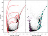 |
Fig. D.1. HST/ACS CMD of the Leo A galaxy shown with black dots. Left panel: theoretical PARSEC isochrones (red curves) used to classify in the range of ages 50 Myr, 100 Myr, 250Myr, 500 Myr, 800 Myr, 1 Gyr, and 5 Gyr, adopting Z = 0.0007, and A814 = 0.039. Right panel: selected young MS stars (magenta triangles) and old stars (cyan squares) in the Leo A H II region FoV. |
Appendix E: Behaviour of chemical evolution models
In Section 4.4, we applied analytic chemical evolution models to explore the evolution of Leo A from 10 Gyr to the present. The equations 3, 4, 5, and 6 describe the gas-phase metallicity, Zg, as a function of the gas fraction, μ, and the effective yield, yeff.
E.1. Comparison of model at fixed yield
Figure E.1 shows the solution of the four models across the full range of gas fractions, 0 < μ < 1 for yeff = 0.02 (solar yield). The closed-box and accretion models are identical at μ > 0.5, suggesting that galaxies which accrete more than half of their stellar mass in gas evolve effectively as closed boxes. By contrast, the leaky-box and gas-regulator models converge at μ > 0.85. At the extreme gas-rich regime (μ > 0.9), all four models produce nearly identical tracks, implying that extremely gas-dominated systems evolve as if no flows are present. The grey vertical bands represent the gas fractions of Leo A today (μ = 0.68 ± 0.05) and 10 Gyr ago (μ = 0.92 ± 0.06).
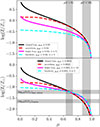 |
Fig. E.1. The gas-phase metallicity as a function of the gas fraction, using the four chemical evolution models. Top panel: all models are reproduced by adopting solar metallicity as yeff (0.02). The closed-box, accretion, leaky-box (λ = 5), and gas-regulator (λ = 5) models are shown with the black solid, red dashed, magenta solid, and cyan dashed curves, respectively. Bottom panel: same models, but using the estimated yeff and λ in Section 4.4 for Leo A. In both panels, the grey vertical bands show the estimated μ at 10 Gyr ago and the present day, whereas the horizontal bands show the stellar and gas-phase metallicities. |
E.2. Behaviour of chemical evolution models with Leo A estimates
The bottom panel of Figure E.1 shows the same comparison using the yeff of Leo A derived by the Monte Carlo simulations. Here, grey horizontal bands are the gas-phase metallicity (−1.65 ± 0.09 dex) and stellar metallicity (−1.23 ± 0.09 dex; Kirby et al. 2017). The same qualitative behaviour is observed as in the top panel: closed-box and accretion models track each other closely, while leaky-box and gas-regulator models converge at high gas fraction but diverge at lower μ.
E.3. The role of the effective yield
The effect of yeff is presented in Figure E.2 for the four models. The colour code presents the yeff evaluated, from 0.001 to 0.02. Varying yeff shifts the intercept of the mass-metallicity curves: higher yields increase the metallicity at fixed gas fractions without altering the curve of the track in the mass-metallicity plane.
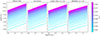 |
Fig. E.2. Comparison of evolutionary tracks between the four chemical evolution models in the mass-metallicity plane. The colour code represents the yeff of each track from 0.001 to 0.02 (solar). Closed-box, accretion, leaky box (λ = 5), and bathtub (λ = 5) are shown in the four panels, from left to right, respectively. |
E.4. The role of the mass-loading factor
Figure E.3 shows the influence of the mass-loading factor, λ, in the leaky-box (left panel) and gas-regulator (right panel) models at yeff = 0.005, the value estimated for Leo A. The colour-code represents the λ values evaluated, from 0 to 35. In this case, increasing λ lowers the intercept and flattens the mass-metallicity curves, reflecting the suppression of enrichment by stronger outflows.
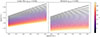 |
Fig. E.3. Comparison of evolutionary tracks between the leaky-box model (left panel) and the bathtub model (right panel) under yeff = 0.005. The colour code represents the mass loading factor (λ) evaluated from 0 to 35. |
E.5. Summary
These experiments clarify why closed-box and accretion models produce similar evolutionary tracks, and why leaky-box and gas-regulator models align under certain regimes. The convergence of all models at high gas fractions explains why gas-rich galaxies behave similarly using chemical evolution models, while the impact of yeff and λ sets the vertical normalisation and the slope of the mass-metallicity tracks for the chemical evolution of Leo A.
All Tables
Integrated emission-line flux measurements in the Leo A H II region, the VZ06 mock slit, and the R18 mock slit spectra.
Electron temperatures, ionic and total oxygen abundances estimates for the Leo A H II region.
All Figures
|
Fig. 1. Subaru Suprime-Cam Hα frame from Stonkutė et al. (2014, 2019). The H II region studied in this work is shown inside the yellow square and represents the VIMOS-IFU FoV. |
| In the text | |
|
Fig. 2. Integrated VIMOS-IFU spectrum of the Leo A H II region normalised by the flux at the peak of the Hβ line. Left panel: spectral window showing Hγ and [O III]λ4363 detection, from left to right, respectively. Middle panel: spectral window presenting the Hβ, and the [O III]λλ 4959,5007 detection, from left to right, respectively. Right panel: spatial distribution of fibres selected to generate the integrated spectrum of the Leo H II region with [O III]λ4363 detection. The colour code represents the jump value of each selected fibre. The grey contours represent the Hβ emission of the nebula as a reference. |
| In the text | |
|
Fig. 3. Emission-line maps of the Leo A H II region. Left panel: Hβ emission-line map. Middle panel: [O III]λ5007 emission-line map. Right panel: Hβ/Hγ map, where the Hβ map contours are superimposed for reference. In all panels, the colour-code represents the flux of the emission lines per spectral fibre acquired by fitting Gaussian curves. The dashed grey lines are circles of increasing radius of 1.34″ (2 px) units up to 13.4″ (20 px). The dotted black lines show the angles that separate the south-western emission clump and the extended arc. |
| In the text | |
|
Fig. 4. Flux-density profiles for the south-western clump and the extended arc in red and blue, respectively. The top panel shows the radial Hβ flux-density profiles for both structures. The upper middle panel shows the radial [O III]λ5007 flux-density profile for both structures. The bottom middle panel shows the Hβ and [O III]λ5007 flux-density profile in purple and green, respectively, for the complete nebula integrated over the entire angular range. The bottom panel shows the Hβ/[O III]λ5007 ratio in black for the complete nebula integrated over the entire angular range. |
| In the text | |
|
Fig. 5. Comparison of Leo A H II region with Hβ emission (grey contours) with HST/ACS photometry. The left panel shows the location of young MS stars (magenta triangles) and old stars (cyan squares). A 10 Myr PARSEC isochrone is shown with the black curve in order to obtain a proxy of the stellar masses of the young stars. The middle panel shows the spatial distribution of old stars in the H II region, whereas the right panel shows the distribution of young MS stars in the H II region. The most massive star is shown with the orange triangle, and those with masses of 8 < M⊙ < 10 are shown with green triangles. |
| In the text | |
|
Fig. 6. Location of stars belonging to C2 star cluster (< 2.5″). Left panel: Location of stars in CMD. The white cross corresponds to the brightest star. The white squares are those stars with 23 < F814W < 24. Stars with F814W > 24 are shown as white dots. Theoretical PARSEC isochrones of 10 Myr, 100 Myr, 250 Myr, 500 Myr, 1 Gyr, and 5 Gyr are shown as colour-coded curves according to their stellar masses given by the theoretical isochrones. K1 and K2 O-type stars from Gull et al. (2022) are shown as the cyan triangle and the cyan diamond, respectively. Those massive stars are capable of ionising individually two Leo A H II regions. Right panel: Location of stars of the C2 star cluster in Leo A H II region (grey contours), superimposed with the HST/ACS F814W frame. |
| In the text | |
|
Fig. 7. Leo A in the mass-metallicity plane, with white square and white dot representing uncorrected and corrected metallicities for Te fluctuations, respectively. The VZ06 (R23) and R18 (Te−based) measures were included as the red triangle and blue square, respectively, for comparison. Dashed and solid black lines are the Lee et al. (2006) and the Berg et al. (2012) low-mass end of the MZR, respectively. The grey crosses and the grey dots are their respective samples. The solid red curve and the dashed red curve are the MZR of the local Universe from Andrews & Martini (2013) and Curti et al. (2020), respectively. |
| In the text | |
|
Fig. 8. Evolution of Leo A over the last 10 Gyr in the mass-metallicity plane. Left panel: White square represents Leo A 10 Gyr ago, whereas the white dot represents Leo A in the present day. The closed-box-model and accretion-model median tracks that approach our estimates are shown as the dotted black and dashed red lines, respectively. The leaky-box and the gas-regulator (bathtub) model median tracks that reproduce our estimates are shown with the solid magenta and the dashed cyan curves, respectively. The closed-box, accretion, leaky-box, and gas-regulator tracks generated by the Monte Carlo simulations are shown with the semi-transparent black, red, magenta, and cyan curves, respectively. Right panel: Same as left panel, but using the Te− corrected gas-phase metallicity as the present-day chemical status of Leo A, shown with the white triangle. |
| In the text | |
|
Fig. A.1. Subaru Suprime-Cam Hα frame from Stonkutė et al. (2014, 2019). The yellow square is the VIMOS-IFU FOV. The cyan line represents the R18 slit position, which goes from H II west (yellow square), to the H II east (red cross). The red line represents the VZ06 slit position. |
| In the text | |
|
Fig. A.2. Integrated spectrum of the Leo A H II region using the VZ06 and R18 mock slits, with red and blue colours, respectively. Left panel: spectral window showing Hγ and [O III]λ4363 detection, from left to right, respectively. Middle panel: spectral window presenting the Hβ, and the [O III]λλ 4959,5007 detection, from left to right, respectively. Right panel: spatial distribution of pixels selected to reproduce both mock slits in the H II region. The grey contours represent the Hβ emission of the nebula for reference. |
| In the text | |
|
Fig. D.1. HST/ACS CMD of the Leo A galaxy shown with black dots. Left panel: theoretical PARSEC isochrones (red curves) used to classify in the range of ages 50 Myr, 100 Myr, 250Myr, 500 Myr, 800 Myr, 1 Gyr, and 5 Gyr, adopting Z = 0.0007, and A814 = 0.039. Right panel: selected young MS stars (magenta triangles) and old stars (cyan squares) in the Leo A H II region FoV. |
| In the text | |
|
Fig. E.1. The gas-phase metallicity as a function of the gas fraction, using the four chemical evolution models. Top panel: all models are reproduced by adopting solar metallicity as yeff (0.02). The closed-box, accretion, leaky-box (λ = 5), and gas-regulator (λ = 5) models are shown with the black solid, red dashed, magenta solid, and cyan dashed curves, respectively. Bottom panel: same models, but using the estimated yeff and λ in Section 4.4 for Leo A. In both panels, the grey vertical bands show the estimated μ at 10 Gyr ago and the present day, whereas the horizontal bands show the stellar and gas-phase metallicities. |
| In the text | |
|
Fig. E.2. Comparison of evolutionary tracks between the four chemical evolution models in the mass-metallicity plane. The colour code represents the yeff of each track from 0.001 to 0.02 (solar). Closed-box, accretion, leaky box (λ = 5), and bathtub (λ = 5) are shown in the four panels, from left to right, respectively. |
| In the text | |
|
Fig. E.3. Comparison of evolutionary tracks between the leaky-box model (left panel) and the bathtub model (right panel) under yeff = 0.005. The colour code represents the mass loading factor (λ) evaluated from 0 to 35. |
| In the text | |
Current usage metrics show cumulative count of Article Views (full-text article views including HTML views, PDF and ePub downloads, according to the available data) and Abstracts Views on Vision4Press platform.
Data correspond to usage on the plateform after 2015. The current usage metrics is available 48-96 hours after online publication and is updated daily on week days.
Initial download of the metrics may take a while.