| Issue |
A&A
Volume 707, March 2026
|
|
|---|---|---|
| Article Number | A313 | |
| Number of page(s) | 13 | |
| Section | Extragalactic astronomy | |
| DOI | https://doi.org/10.1051/0004-6361/202555381 | |
| Published online | 16 March 2026 | |
The X-ray properties of the most luminous quasars with strong emission-line outflows
1
Instituto de Astrofísica, Facultad de Física, Pontificia Universidad Católica de Chile, Casilla 306, Santiago 22, Chile
2
Dipartimento di Fisica e Astronomia, Università degli Studi di Firenze, via G. Sansone 1, 50019 Sesto Fiorentino, Firenze, Italy
3
INAF – Osservatorio Astrofisico di Arcetri, Largo E. Fermi 5, 50125 Firenze, Italy
4
Scuola Normale Superiore, Piazza dei Cavalieri 7, I-56126 Pisa, Italy
5
Dipartimento di Matematica e Fisica, Univeristà di Roma 3, Via della Vasca Navale, 84, 00146 Roma RM, Italy
6
European Space Agency (ESA), European Space Research and Technology Centre, Noordwijk, The Netherlands
7
Instituto de Alta Investigación, Universidad de Tarapacá, Casilla 7D Arica, Chile
8
Centre for Extragalactic Astronomy, Department of Physics, Durham University, South Road, Durham DH1 3LE, UK
9
Institute for Astronomy, University of Edinburgh, Royal Observatory, Blackford Hill, Edinburgh EH9 3HJ, UK
10
Department of Physics, Drexel University, 32 S. 32nd Street, Philadelphia, PA 19104, USA
★ Corresponding author: This email address is being protected from spambots. You need JavaScript enabled to view it.
Received:
4
May
2025
Accepted:
19
November
2025
Abstract
Context. Strong outflows from active galactic nuclei are frequently observed in objects with lower coronal X-ray luminosity. This intrinsic X-ray weakness is considered a requirement for the formation of radiatively driven winds.
Aims. To obtain an unbiased view on the connection between X-ray emission and the presence of powerful winds in the most luminous quasar phase, we present an X-ray analysis of a sample of extremely luminous, radio-quiet quasars with signatures of strong outflows in their rest-frame ultraviolet (UV) emission spectra.
Methods. We study the Chandra X-ray spectral properties of 10 objects, selected from the Sloan Digital Sky Survey Data Release 16 quasar catalogue based on their UV luminosities and C IV emission line blueshifts, comparing them to typical optically blue quasars.
Results. Our analysis reveals that seven out of 10 quasars in our sample have photon indices Γ > 1.7. Only two out of 10 objects exhibiting outflows with velocities exceeding 1400 km/s are X-ray ‘weak’, consistent with the fraction of X-ray ‘weak’ objects generally observed in quasar populations. Notably, one of the objects identified as X-ray ‘weak’ is likely an intrinsically X-ray ‘normal’ quasar that is heavily obscured. We observe a tentative indication at a ∼2σ confidence level that the correlation between the excessively low X-ray flux level and the presence of C IV emission-line outflows might emerge at wind velocities greater than 3000 km/s.
Conclusions. Our study provides additional evidence that the relationship between X-ray emission and the presence of winds is intricate. Our findings emphasise the need for X-ray observations of a larger sample of UV-selected quasars with confirmed strong emission-line outflows to unravel the nuanced interplay between winds and X-ray emission.
Key words: methods: observational / techniques: spectroscopic / galaxies: nuclei / X-rays: general / quasars: general
© The Authors 2026
 Open Access article, published by EDP Sciences, under the terms of the Creative Commons Attribution License (https://creativecommons.org/licenses/by/4.0), which permits unrestricted use, distribution, and reproduction in any medium, provided the original work is properly cited.
This article is published in open access under the Subscribe to Open model. This email address is being protected from spambots. You need JavaScript enabled to view it. to support open access publication.
1. Introduction
Active galactic nuclei (AGNs) are actively accreting supermassive black holes (SMBHs) at the centres of some galaxies. AGN-driven outflows are considered the leading explanation for the co-evolution of SMBHs and their host galaxies (e.g. Zubovas & King 2012; Faucher-Giguère & Quataert 2012; Kormendy & Ho 2013). Evidence supporting this co-evolution comes from well-established correlations between SMBH mass and various host galaxy properties, including bulge mass, luminosity, and velocity dispersion (e.g. Magorrian et al. 1998; Ferrarese & Merritt 2000; Gebhardt et al. 2000; Tremaine et al. 2002; Häring & Rix 2004). Quasars, the most luminous class of AGNs, are expected to produce outflows powerful enough to rapidly suppress star formation, therefore regulating galaxy evolution (e.g. Cano-Díaz et al. 2012; Fabian 2012; King & Pounds 2015; Davies et al. 2020, 2024).
The existence of high-velocity outflows with large column density, arising as a natural consequence of efficient SMBH accretion, is a robust prediction of theoretical models (King & Pounds 2003) and numerical simulations (Takeuchi et al. 2013; Matthews et al. 2023). Observational evidence for these powerful outflows is found in both the ultraviolet (UV) and X-ray spectra. In the UV range, broad absorption lines (BALs) that are blueshifted by several thousand km/s are present in the spectra of > 20% of quasars (Hewett & Foltz 2003; Trump et al. 2006; Gibson et al. 2009; Allen et al. 2011; Bischetti et al. 2023). Ultra-fast outflows (UFOs) with blueshifts exceeding 10 000 km/s are observed in the X-ray spectra of ∼30–40% of quasars (Tombesi et al. 2010; Gofford et al. 2013).
Although AGN feedback via outflows is widely accepted as a mechanism driving the co-evolution of SMBHs and their host galaxies, any conclusive confirmation is still lacking (see Harrison 2017, and references therein). Additionally, a definitive understanding of the relationship between the presence of outflows and the steepness of the UV-to-X-ray spectral energy distribution of quasars remains elusive. On the one hand, intrinsic X-ray weakness is generally considered a prerequisite for the presence of winds, as it mitigates over-ionisation and facilitates line driving (Murray et al. 1995; Proga et al. 2000; Proga & Kallman 2004; Higginbottom et al. 2014, 2024; Dyda et al. 2024). On the other hand, evidence suggests that in the Eddington-limited accretion regime, X-ray weakness may also be a consequence of winds (see Figure 13 in Trefoloni et al. 2023). For instance, the X-ray-weak sample of Nardini et al. (2019) might be characterised by a higher incidence of excessive UV/optical outflows, as suggested by C IV emission line profiles with larger velocity shifts and prominent blue wings (Lusso et al. 2021; see also Zappacosta et al. 2020 for additional evidence).
Quasars exhibiting strong absorption signatures from winds are often observed to be X-ray ‘weak’ (Gallagher et al. 2002, 2006; Stalin et al. 2011). This weakness is typically quantified by comparing the observed X-ray luminosity to that predicted by the X-ray-to-UV luminosity relation observed in ‘normal’ blue quasars (e.g. Lusso et al. 2020, hereafter L20). Simultaneously, while the features mentioned above provide a direct means of detecting AGN winds, they necessitate a line of sight through the outflowing gas, introducing an inherent bias due to significant modifications in the observed spectra. The faintness of modified spectra makes it unclear whether the observed X-ray weakness is intrinsic or a result of absorption along the line of sight. This ambiguity complicates the inference of how the winds influence the relationship between UV and X-ray luminosities.
The method to circumvent the aforementioned bias and assess the general connection between X-ray emission and the presence of extreme winds in quasars is to utilise emission lines in UV spectra as a means of detecting AGN winds. Several previous studies attempted to infer the influence of the outflow velocities, parametrised by the blueshift of the C IV broad emission line, on the relationship between UV and X-ray luminosities (e.g. Gibson et al. 2008; Kruczek et al. 2011; Ni et al. 2018; Zappacosta et al. 2020; Timlin et al. 2020; Rivera et al. 2022; Temple et al. 2023); nevertheless, the findings remain inconclusive. The only way to obtain an unbiased view of the connection between outflows and X-ray properties of quasars is to perform an X-ray analysis of UV-selected sources without any prerequisites on their X-ray characteristics.
In this paper, we present the X-ray analysis of 10 quasars, selected from the Sloan Digital Sky Survey (SDSS) Data Release 16 (DR16) quasar catalogue (Lyke et al. 2020), which exhibit evidence of strong outflows in their C IV emission line. We compare these objects with the L20 sample of typical optically selected blue quasars and examine the connection between X-ray emission properties and the presence of powerful winds in the highly luminous quasar phase. The paper is structured as follows. In Section 2, we describe the sample selection, whilst the X-ray data analysis is reported in Section 3. We present and discuss the results of the X-ray-to-UV luminosity relation fitting in Section 4, and conclusions are drawn in Section 5.
For simplicity, here we adopt a standard flat ΛCDM cosmology with ΩM = 0.3 and H0 = 70 km s−1 Mpc−1.
2. Sample selection
2.1. The main dataset
The incidence of blueshifted broad emission lines indicates a prevalence of fast outflows at high luminosities (Richards et al. 2011). This prevalence is further supported by an analysis of the spectral properties of quasars in the SDSS DR16 catalogue, available in Wu & Shen (2022). Figure 1 shows the centroid shift of the C IVλ1549 Å emission line as a function of the UV luminosity at 2500 Å. The centroid shift of the C IV line is defined as the difference between its measured 50% flux centroid wavelength (i.e. the wavelength that divides the line into two parts with equal flux) and the rest-frame wavelength. We restricted our analysis to the redshift interval of z = 1.8 − 2.2. The lower boundary of z > 1.8 ensures that the C IV line is included within the SDSS spectra. The upper boundary of z < 2.2 is justified by the requirement for the presence of the Mg IIλ2800 Å emission line in the SDSS spectra, which, along with the C III] λ1909 Å, provides a reliable redshift measurement independent of the C IV line. The distribution of the C IV centroid shifts is roughly symmetric at lower luminosities, whereas significant blueshifts are observed in nearly all sources at the highest luminosities. Therefore, we pre-selected our targets based on their UV luminosity at 2500 Å and the centroid shift of the C IV emission line.
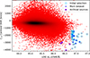 |
Fig. 1. Shift of centroid of C IVλ1549 Å line in units of km/s, as function of logarithmic luminosity νLν at 2500 Å, available in Wu & Shen (2022). The sample consists of all the quasars in the SDSS DR16 sample with redshift in the z = 1.8–2.2 interval, colour-coded from red to black by the density of the underlying points. Empty cyan circles indicate 45 objects pre-selected for the one-by-one modelling of the C IV line with multiple components. Filled semi-transparent blue circles show a subset of 10 objects with the confirmed strongly blueshifted component, the main dataset analysed in this paper. Violet circles show four supplementary archival sources. |
We focused on the most luminous, highly accreting quasars with a UV luminosity at 2500 Å of log (νLν/erg s−1) > 46.8. With a standard bolometric correction from the 2500 Å luminosity of ∼4–5, this criterion corresponds to a bolometric luminosity exceeding the Eddington luminosity for a 109 M⊙ black hole. We then selected the sources with a centroid blueshift greater than 1400 km/s (see Figure 1).
The SDSS DR16 catalogue does not include information on fitting the C IV line with multiple Gaussian components, but rather provides the measurements for the whole line profile. Therefore, the selection process outlined above relied on outflow velocities estimated from the centroid shifts of the full C IV line. Moreover, the distribution of the C IV blueshifts depends on the combination of the schemes used to determine the quasar redshifts and to quantify the line properties (see Figure 1 in Coatman et al. 2016). To confirm that the blueshifts of the 50% flux centroid are indeed due to the presence of a strongly blueshifted component in the emission line, we conducted a detailed individual analysis of the SDSS spectra of 45 pre-selected sources, modelling the C IV line with multiple components (see Figure 2 and Appendix A for further details). We also excluded radio-loud quasars from our sample. C IV outflow velocities, reported in Table 2, were measured in our modelling of the C IV line as the shift of the outflow component with respect to the broad line region (BLR) component. Since the bulk of the BLR emission for the C IV line in such bright sources could likely be itself in outflow (see, e.g. Vietri et al. 2018; and also Figure 2), this approach to calculating the outflow velocity should be regarded as conservative. We additionally calculated outflow velocities non-parametrically as the difference between the wavelength corresponding to the bluest tenth percentile of the line and the wavelength corresponding to the line’s peak.
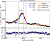 |
Fig. 2. Example of analysis of C IV spectral region of SDSS spectra. The fitted lines are reported as labels. The components employed in the fit are colour-coded, as shown in the legend. The reported C IV outflow velocity is measured as the shift of the outflow component with respect to the BLR component. The dashed vertical lines indicate the expected position for the fitted lines according to the redshift reported in the catalogue. The shaded light grey regions are telluric bands, narrow absorption lines, or bad pixels and are therefore excluded from the fit. See Appendix A for the analysis of other sources. |
We further confirmed the presence of outflows using C IV emission line blueshifts calculated from spectral reconstructions based on a mean-field independent component analysis (MFICA) scheme (Rankine et al. 2020; Temple et al. 2023). In this approach, the C IV blueshift is defined as the Doppler shift of the wavelength bisecting the continuum-subtracted line flux (i.e. the rest-frame wavelength of the observed line centroid) with respect to the mean rest-frame wavelength of the C IV doublet, obtained using the improved redshift estimation. Improved redshifts were obtained from P. Hewett (private communication and Hewett et al., in prep.). The scheme used 27 high signal-to-noise ratio templates in a fashion similar to that described in Section 2.1 of Stepney et al. (2023). A key difference, however, is that the templates and spectra were cross-correlated (see Equation (1) of Hewett & Wild 2010) using a wavelength range restricted to rest-frame 1700 –3000 Å. Constraining the match to include only the C III] λ1909 Å emission complex and Mg IIλ2800 Å emission avoids biases that arise from the presence of C IV absorbers in the blue wing of the C IV emission line. All objects selected in the aforementioned process have C IV blueshifts measured from MFICA reconstructions greater than 1700 km/s. Figure 3 shows MFICA reconstructed C IV blueshifts and equivalent widths (EWs), and He II EWs of the selected objects in relation to those of the z = 1.8 − 2.2 quasars in the SDSS DR16 sample.
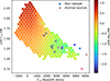 |
Fig. 3. C IV emission space with hexagons colour-coded by median He II EW for 66810 quasars in SDSS DR16 sample with redshift in z = 1.8 − 2.2 interval, having reliable C IV and He II measurements from MFICA reconstructions. Only hexagons with five or more quasars are plotted. Circles colour-coded by corresponding He II EW show the main dataset of 10 objects and four supplementary archival sources. |
The main dataset presented in this paper consists of 10 sources. Table 1 provides the corresponding observing parameters of the X-ray data. Source SDSS J073502.30+265911.5 was observed by the Chandra X-ray Observatory in October 2015 (cycle 16, proposal ID: 16700345, PI: E. Piconcelli). The Advanced CCD Imaging Spectrometer (ACIS) instrument operated in VFAINT TE mode, with an on-source time of 24.75 ks. This object is part of the WISSH quasars sample (Martocchia et al. 2017), but we performed a complete reprocessing and data analysis to ensure the homogeneity of measurements across the main dataset. The Chandra observations of the remaining nine quasars in our sample are proprietary and previously unpublished. Observations began in December 2023 and were completed in August 2025 (cycle 25, proposal ID: 25700372, PI: G. Risaliti). For each target, the ACIS instrument operated in FAINT TE mode, with on-source times ranging from 10.93 to 18.83 ks. The observation data files were reprocessed using the Chandra Interactive Analysis of Observations (CIAO) software package (CIAO Development Team 2013) v4.16.0 and the Chandra calibration database (CalDB) v4.11.2, applying the point-source aperture correction to the unweighted auxiliary response files.
Observing parameters of X-ray data.
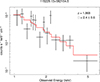 |
Fig. 4. Example of analysis of Chandra X-ray spectra. To enhance visual clarity, the spectrum in the plot is binned to ensure at least 1.5 counts per energy channel. Black crosses represent the observational data with corresponding errors, red line represents the best-fit model. See Appendix B for the analysis of other sources. |
2.2. Supplementary archival data
We find no significant evidence for a correlation between the excessively low X-ray flux level of quasars and the presence of outflows in our main dataset (see Section 4.2 for details). Therefore, we also considered a control sample to check whether any such correlation emerges at a higher velocity threshold.
We searched through the Chandra and XMM-Newton archives for observed highly luminous quasars that exhibit a C IV centroid blueshift, calculated from the spectral properties reported by Wu & Shen (2022), greater than 3000 km/s. We expanded the redshift interval to z = 1.7 − 2.4, relaxed our UV luminosity criterion to log (νLν/erg s−1) > 46.3 at 2500 Å, and identified four additional sources with available X-ray observations (see Table 1 for the observing parameters). SDSS J082508.75+115536.3 and SDSS J122048.52+044047.6 were observed with Chandra (Luo et al. 2015; Ni et al. 2018). Their rest-frame monochromatic luminosities at 2 keV were calculated based on the reported rest-frame 2-keV flux densities (see Table 2). We acknowledge that SDSS J082508.75+115536.3 was targeted as a likely X-ray ‘weak’ object and SDSS J122048.52+044047.6 as a potentially X-ray ‘weak’ one, which possibly introduces a bias into our control sample. SDSS J092156.38+285237.7 and SDSS J104350.35+140703.0 were located in the 4XMM-DR14 Serendipitous Source Catalogue (Traulsen et al. 2020). In order to obtain a homogeneous analysis, we reduced these two XMM-Newton sources following the standard procedure outlined in the European Space Agency’s XMM-Newton web pages, and we performed a spectral analysis analogous to the one described for Chandra sources (see Section 3 for details).
Optical properties and results of C IV region and X-ray spectral analysis.
MFICA reconstructed C IV blueshifts of these supplementary archival objects are greater than 3200 km/s. We further confirmed the presence of a strongly blueshifted component in the C IV emission line and measured outflow velocities by modelling the line with multiple components, similar to the sources in our main dataset.
3. X-ray data analysis
The spectral analysis of the main dataset was conducted using the general X-ray spectral-fitting program XSPEC (Arnaud et al. 1999) v12.14.0. We re-binned the data to ensure that there was at least one count per energy channel and employed the C-statistic (Cash 1979; Kaastra 2017), which is more appropriate for the low-count Poissonian regime. The reported uncertainties correspond to a change in the fit statistics of ΔC = 2.706 (equivalent to the 90% confidence level in the Gaussian approximation).
Despite the limited quality of the obtained spectra, we achieved a robust estimation of the X-ray flux for all sources in our sample, except for one with a non-detection (see Figure 4 and Appendix B). The spectra were fitted over the 0.3–8 keV energy range, as virtually no source counts were detected outside this range. The initially adopted spectral model consisted of a power-law continuum modified by Galactic absorption from HI4PI Collaboration (2016), as well as absorption in the vicinity of the sources. In XSPEC terminology, this is expressed as phabs × zphabs × powerlw. We found that the non-Galactic H I column density is log NH < 21.5, with ΔC = 3.84 (equivalent to the 95% confidence level in the Gaussian approximation), for all sources in our main dataset, except for one with a non-detection. Therefore, for further analysis, we fixed the non-Galactic absorption parameter to zero. Consequently, our resulting spectral model included only two free parameters: the photon index of the power law and the flux, assessed through cflux in XSPEC (which has been omitted from the model definition above for simplicity).
For each source in the main dataset with a detection, we determined the observed-frame 1–10 keV flux and estimated the monochromatic rest-frame 2-keV luminosity. The inferred power-law photon indices, measured fluxes, and estimated luminosities are provided in Table 2. In the case of SDSS J111800.50+195853.4, we additionally estimated the rest-frame 2-keV luminosity assuming the source to be an X-ray steep but heavily obscured quasar, by allowing the non-Galactic absorption parameter to vary while fixing the photon index at Γ = 2.0, the average photon index for a blue quasar (e.g. Bianchi et al. 2009; Young et al. 2009). This analysis resulted in the non-Galactic H I column density of  and monochromatic rest-frame 2-keV luminosity of log L2 keV = 27.8 ± 0.2. In the case of SDSS J133610.96+184529.9, the only source for which the count rate in the 0.3–8 keV energy range corresponds to a non-detection, we fixed the model by setting the non-Galactic absorption parameter to zero and the photon index to Γ = 2.0. With the resulting model having only the flux as a free parameter, we estimated upper limits of the observed-frame 1–10 keV flux and the monochromatic rest-frame 2-keV luminosity at a 90% confidence level. The measured values are consistent with those obtained using confidence limits from Kraft et al. (1991).
4. Results
4.1. Photon index distribution
It is essential to consider the possibility of intrinsic X-ray absorption when investigating the X-ray properties of quasars. In order to disentangle intrinsic X-ray weakness from the presence of absorption, particularly in cases where the fit returns low non-Galactic H I column densities, the continuum photometric photon index, Γ, can be utilised (Rivera et al. 2022). Objects with flatter X-ray spectra than the average (i.e. low photon index) are likely affected by absorption, while those observed as X-ray ‘weak’ with relatively steep X-ray spectra are likely intrinsically X-ray weak (see Figures 1 and 2 in Giustini & Proga 2019). Therefore, we compare the continuum photon indices of objects in our main dataset with those in the L20 parent sample.
In the L20 parent sample, prior to applying the photon index selection criterion, the distribution of photon indices has a mean value of 1.94 and a standard deviation of 0.45. Our main dataset has a distribution of photon indices with a mean value of 2.04 and a standard deviation of 0.42. These properties of the distribution indicate that, on average, our sources reside among quasars with steep X-ray spectra, suggesting very low intrinsic X-ray absorption. Notably, we find that seven out of 10 objects in our sample have X-ray spectra with photon indices Γ > 1.7 (see Table 2). Considering that quasars in our sample exhibit a strongly blueshifted C IV emission line with moderate to low EW (see Figure 3), this result is consistent with previous studies indicating that objects with high C IV blueshifts and low C IV EWs tend to have steep X-ray spectra (e.g. Gallagher et al. 2005; Kruczek et al. 2011; Rivera et al. 2022).
4.2. LX–LUV relation
The L20 sample is suitable for cosmological applications that utilise a quasar Hubble diagram, where luminosity distances are derived from the X-ray-to-UV luminosity relation (e.g. Risaliti & Lusso 2015, 2019; Lusso et al. 2019). Due to the selection criteria in L20, aimed at isolating the quasars with reliable measurements of intrinsic UV and X-ray emission, the dispersion in the LX–LUV relation obtained from that sample is as low as 0.2 dex. Therefore, the L20 sample can be regarded as consisting of X-ray ‘normal’ optically blue quasars. Consequently, we evaluated the X-ray intensity of the objects in our sample by comparing their luminosities to those expected from the LX–LUV relation established for the L20 sample.
We determined the slope γ, intercept, and dispersion δ of the X-ray-to-UV luminosity relation for the L20 sample using the Python package EMCEE (Foreman-Mackey et al. 2013), a pure-Python implementation of Goodman & Weare’s affine invariant Markov chain Monte Carlo (MCMC) ensemble sampler. The regression fit was conducted with the normalisation of X-ray and UV luminosities set to the respective median values of the analysed sample.
Figure 5 demonstrates that eight out of 10 quasars in our main dataset are X-ray ‘normal’ within ΔC = 3.84 and the 3σ dispersion of the LX–LUV relation. The only two X-ray ‘weak’ quasars are J111800.50+195853.4 and J133610.96+184529.9. J111800.50+195853.4 is an outlier of the X-ray-to-UV luminosity relation at 6σ. J133610.96+184529.9 has an upper limit below the X-ray-to-UV luminosity relation at 5σ. For seven objects in our main dataset with Γ > 1.7, we additionally examined the X-ray-to-UV luminosity relation in narrow redshift bins. We confirmed that these objects are X-ray ‘normal’ within ΔC = 2.706 and the 2σ dispersion of the relation in their respective redshift bins (see Appendix C for further details). Therefore, our main dataset of the most luminous quasars contains two X-ray ‘weak’ objects out of 10, which aligns with the average expectation for quasar populations. Cautious about the small size of our sample, we estimated the statistical uncertainty for the fraction of X-ray ‘weak’ objects using the Clopper-Pearson method (Clopper & Pearson 1934), which conservatively guarantees that the interval coverage is always equal to or above the confidence level (e.g. Brown et al. 2001). The 68% confidence interval for the true fraction is 10.6–32.0%. Furthermore, if we assume J111800.50+195853.4 to be a heavily obscured quasar with an intrinsic continuum photon index of Γ = 2.0, its estimated monochromatic rest-frame 2-keV luminosity becomes consistent with that of X-ray ‘normal’ quasars within the 2σ dispersion of the LX–LUV relation, bringing the mean fraction of intrinsically X-ray ‘weak’ objects down to one out of 10 and the 68% confidence interval for the true fraction to 1.6–26.3%.
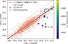 |
Fig. 5. Rest-frame monochromatic luminosities LX against LUV for 10 quasars in our main dataset and four additional quasars from Chandra and XMM-Newton archives, colour-coded by C IV outflow velocity in units of km/s, measured in our modelling of C IV line as the shift of the outflow component with respect to the BLR component. Colour-coded and empty black squares show modelling of J111800.50+195853.4 with a free and fixed photon index, respectively. Downward arrows indicate non-detection, and the corresponding squares represent upper limits. Light red dots represent the sample of about 2000 quasars from Lusso et al. (2020), with the relative regression line in red, for which the slope γ, with its error, and the dispersion δ are specified. The dashed and dotted lines trace the 1σ and 3σ dispersion, respectively. |
Considering the high uncertainty in the C IV outflow velocities measured in our analysis of the SDSS spectra for some sources in our sample (see Table 2), we repeated the examination of a possible correlation between the X-ray flux level of quasars and the presence of outflows using different methods to measure the outflow velocity. We used outflow velocities that we measured non-parametrically, shifts of the centroid of the C IV line, reported by Wu & Shen (2022), and those measured from MFICA reconstructions. Despite the discrepancy between the values of the outflow velocity measured using different methods for each particular source, our results remain consistent, showing no significant evidence of a correlation between the excessively low X-ray flux level and the presence of strong winds in the most luminous quasar phase. At the same time, the position of our sample within the C IV emission space (see Figure 3) corresponds to the regime dominated by an efficient radiation line-driven disc wind, expected to occur in cases of high black hole mass and high mass-normalised accretion rates (Temple et al. 2023), which aligns with the luminosity characteristics of our sample. Relatively low He II EWs of quasars in our sample suggest a weak extreme UV ionising emission compared to the UV continuum (Timlin et al. 2021), which is required to avoid over-ionising the gas responsible for line driving. Therefore, He II EWs support the possibility for our objects to efficiently launch a radiation-driven wind without the necessity for excessive steepness of the UV-to-X-ray spectral energy distribution (Temple et al. 2023). Our findings align with previous studies (e.g. Timlin et al. 2020; Rivera et al. 2022), providing supplementary evidence of the complexity of the relationship between X-ray emission and the presence of winds in luminous quasars.
It is worth noting that this absence of correlation between the excessive steepness of the UV-to-X-ray spectral energy distribution and the presence of strong winds could be explained by the non-simultaneity of the X-ray and UV observations used in our analysis. Our objects could have been X-ray ‘weak’ during the outflow phase, which was concealed by variations in X-ray and UV properties between the corresponding observations due to intrinsic variability in quasars. Alternatively, the reason may lie in the difference between the ionising continuum seen by the BLR and in our observations (see, e.g. Section 2.3 in Leighly 2004), or the fact that the C IV blueshifts have some orientation dependence rather than solely reflecting outflow velocities (see, e.g. Richards et al. 2021). The relative locations of the accretion disk, the BLR, and the X-ray corona with respect to each other and our line of sight could influence the observed C IV emission line profiles, at the same time contributing to the X-ray weakness at higher inclinations.
Finally, we evaluated the probability that the correlation between the excessively low X-ray intensity in the most luminous quasar phase and the presence of strong outflows might emerge at a higher velocity threshold. We supplemented our main dataset with archival data and divided the sample into two subsets. The first subset includes five quasars exhibiting blueshift of the centroid of the C IV line, reported by Wu & Shen (2022), greater than 3000 km/s, of which two objects we identified as X-ray ‘weak’. The second subset includes the remaining nine quasars, of which only one was identified as X-ray ‘weak’. The probability that the two subsets have the same underlying fraction of X-ray ‘weak’ sources is Pnull = 0.012. This null hypothesis probability corresponds to a 2.5σ confidence level for the presence of a correlation between the excessively low X-ray flux level and outflows faster than 3000 km/s. If we assume J111800.50+195853.4 to be a heavily obscured X-ray ‘normal’ quasar, the null hypothesis probability becomes Pnull = 0.062, corresponding to a 1.9σ confidence level for the presence of a correlation. Therefore, we do not claim any correlation between the X-ray properties and the presence of strong outflows in the most luminous quasar phase based on our small sample, but note that there is a hint at a ∼2σ level that the correlation might emerge for winds faster than 3000 km/s. A larger sample is required to understand whether the correlation between the two phenomena is due to a statistical fluctuation or a physical effect.
5. Conclusions
We have presented an X-ray analysis of a sample of 10 extremely luminous, radio-quiet, non-BAL quasars with evidence of strong outflows in their rest-frame UV emission spectra. This sample was selected from the SDSS DR16 quasar catalogue based on optical/UV characteristics, without any prerequisites regarding X-ray properties. The presence of strong outflows, parametrised by the blueshift of the C IV broad emission line, was confirmed in a one-by-one analysis of the SDSS spectra of the sources. We analysed the X-ray properties of the sample and compared them with those of a sample of typical optically selected blue quasars. Our main findings can be summarised as follows:
-
The photon indices for quasars in our main dataset show that our sources mostly exhibit X-ray steep spectra. We find that seven out of 10 objects have photon indices Γ > 1.7, and are therefore unlikely to be absorbed.
-
Only two out of 10 highly luminous quasars with C IV emission-line outflows exceeding 1400 km/s are X-ray ‘weak’, compared to predictions from the X-ray-to-UV luminosity relation. This result is consistent with the average fraction observed in quasar populations overall. One of the objects identified as X-ray ‘weak’ is possibly an intrinsically X-ray ‘normal’, yet heavily obscured, quasar.
-
We observe a tentative indication of the correlation between the excessively low X-ray intensity and the presence of C IV emission-line outflows that exceed 3000 km/s at a ∼2σ confidence level. However, a larger sample is required to determine whether this finding results from a statistical fluctuation or reflects a physical effect.
The steepness of X-ray spectra in our sample of extremely luminous quasars with C IV emission-line outflows exceeding 1400 km/s, along with the fact that most of our objects follow the LX–LUV relation of typical optically blue quasars, is consistent with previous studies. Our results contribute to the body of evidence indicating that the relationship between X-ray emission and the presence of winds in luminous quasars is complicated and perplexing.
Given the probabilistic nature of our results, extending X-ray observations to larger samples of UV-selected quasars with confirmed high-velocity outflows will be important. These observations will help disentangle the different processes affecting the C IV blueshifts and clarify the complex interplay between outflows and X-ray emission in quasars.
Acknowledgments
This research has utilised data obtained from the 4XMM XMM-Newton serendipitous stacked source catalogue 4XMM-DR14, compiled by the institutes of the XMM-Newton Survey Science Centre selected by ESA. The authors are grateful to the anonymous referee for useful and constructive comments. We thank the Munich Institute for Astro-, Particle, and BioPhysics (MIAPbP), which is funded by the Deutsche Forschungsgemeinschaft (DFG, German Research Foundation) under Germany’s Excellence Strategy – EXC-2094 – 390783311, for providing space for fruitful discussions on this work. AS is supported by the national doctoral scholarship from the Agencia Nacional de Investigación y Desarrollo (ANID), folio de postulación 21221788. AS personally acknowledges Olesya and Kirill Kuchay for their unwavering support. BT acknowledges support by the European Union’s HE ERC Starting Grant No. 101040227 – WINGS. Views and opinions expressed are, however, those of the authors only and do not necessarily reflect those of the European Union or the European Research Council Executive Agency. Neither the European Union nor the granting authority can be held responsible for them. MJT acknowledges funding from the UKRI grant ST/X001075/1. ALR acknowledges funding from a Leverhulme Early Career Fellowship. We gratefully acknowledge funding from ANID – Millennium Science Initiative – AIM23-0001 and ICN12_009 (FEB), CATA-BASAL – FB210003 (FEB), and FONDECYT Regular – 1241005 (FEB). Support for this work was also provided in part by the National Aeronautics and Space Administration through Chandra Award Numbers GO4-25074X and AR1-22010X issued by the Chandra X-ray Centre, which is operated by the Smithsonian Astrophysical Observatory for and on behalf of the National Aeronautics and Space Administration under contract NAS8-03060 and upon work supported by NASA under award 80NSSC24K0719.
References
- Allen, J. T., Hewett, P. C., Maddox, N., Richards, G. T., & Belokurov, V. 2011, MNRAS, 410, 860 [NASA ADS] [CrossRef] [Google Scholar]
- Arnaud, K., Dorman, B., & Gordon, C. 1999, Astrophysics Source Code Library [record ascl:9910.005] [Google Scholar]
- Bianchi, S., Guainazzi, M., Matt, G., Fonseca Bonilla, N., & Ponti, G. 2009, A&A, 495, 421 [NASA ADS] [CrossRef] [EDP Sciences] [Google Scholar]
- Bischetti, M., Fiore, F., Feruglio, C., et al. 2023, ApJ, 952, 44 [NASA ADS] [CrossRef] [Google Scholar]
- Brown, L. D., Cai, T. T., & DasGupta, A. 2001, Stat. Sci., 16, 101 [Google Scholar]
- Cano-Díaz, M., Maiolino, R., Marconi, A., et al. 2012, A&A, 537, L8 [NASA ADS] [CrossRef] [EDP Sciences] [Google Scholar]
- Cash, W. 1979, ApJ, 228, 939 [Google Scholar]
- CIAO Development Team 2013, Astrophysics Source Code Library [record ascl:1311.006] [Google Scholar]
- Clopper, C. J., & Pearson, E. S. 1934, Biometrika, 26, 404 [Google Scholar]
- Coatman, L., Hewett, P. C., Banerji, M., & Richards, G. T. 2016, MNRAS, 461, 647 [NASA ADS] [CrossRef] [Google Scholar]
- Davies, R. L., Förster Schreiber, N. M., Lutz, D., et al. 2020, ApJ, 894, 28 [NASA ADS] [CrossRef] [Google Scholar]
- Davies, R. L., Belli, S., Park, M., et al. 2024, MNRAS, 528, 4976 [CrossRef] [Google Scholar]
- Dickey, J. M., & Lockman, F. J. 1990, ARA&A, 28, 215 [Google Scholar]
- Dyda, S., Davis, S. W., & Proga, D. 2024, MNRAS, 530, 5143 [Google Scholar]
- Fabian, A. C. 2012, ARA&A, 50, 455 [Google Scholar]
- Faucher-Giguère, C.-A., & Quataert, E. 2012, MNRAS, 425, 605 [Google Scholar]
- Ferland, G. J., Porter, R. L., van Hoof, P. A. M., et al. 2013, Rev. Mex. Astron. Astrofis., 49, 137 [Google Scholar]
- Ferrarese, L., & Merritt, D. 2000, ApJ, 539, L9 [Google Scholar]
- Foreman-Mackey, D., Conley, A., Meierjurgen Farr, W., et al. 2013, Astrophysics Source Code Library [record ascl:1303.002] [Google Scholar]
- Gallagher, S. C., Brandt, W. N., Chartas, G., & Garmire, G. P. 2002, ApJ, 567, 37 [CrossRef] [Google Scholar]
- Gallagher, S. C., Richards, G. T., Hall, P. B., et al. 2005, AJ, 129, 567 [Google Scholar]
- Gallagher, S. C., Brandt, W. N., Chartas, G., et al. 2006, ApJ, 644, 709 [Google Scholar]
- Gebhardt, K., Bender, R., Bower, G., et al. 2000, ApJ, 539, L13 [Google Scholar]
- Gibson, R. R., Brandt, W. N., & Schneider, D. P. 2008, ApJ, 685, 773 [NASA ADS] [CrossRef] [Google Scholar]
- Gibson, R. R., Jiang, L., Brandt, W. N., et al. 2009, ApJ, 692, 758 [Google Scholar]
- Giustini, M., & Proga, D. 2019, A&A, 630, A94 [NASA ADS] [CrossRef] [EDP Sciences] [Google Scholar]
- Gofford, J., Reeves, J. N., Tombesi, F., et al. 2013, MNRAS, 430, 60 [Google Scholar]
- Häring, N., & Rix, H.-W. 2004, ApJ, 604, L89 [Google Scholar]
- Harrison, C. M. 2017, Nat. Astron., 1, 0165 [NASA ADS] [CrossRef] [Google Scholar]
- Hewett, P. C., & Foltz, C. B. 2003, AJ, 125, 1784 [NASA ADS] [CrossRef] [Google Scholar]
- Hewett, P. C., & Wild, V. 2010, MNRAS, 405, 2302 [NASA ADS] [Google Scholar]
- HI4PI Collaboration (Ben Bekhti, N., et al.) 2016, A&A, 594, A116 [NASA ADS] [CrossRef] [EDP Sciences] [Google Scholar]
- Higginbottom, N., Proga, D., Knigge, C., et al. 2014, ApJ, 789, 19 [NASA ADS] [CrossRef] [Google Scholar]
- Higginbottom, N., Scepi, N., Knigge, C., et al. 2024, MNRAS, 527, 9236 [Google Scholar]
- Hiremath, P., Rankine, A. L., Aird, J., et al. 2025, MNRAS, 542, 2105 [Google Scholar]
- Kaastra, J. S. 2017, A&A, 605, A51 [NASA ADS] [CrossRef] [EDP Sciences] [Google Scholar]
- Kalberla, P. M. W., Burton, W. B., Hartmann, D., et al. 2005, A&A, 440, 775 [NASA ADS] [CrossRef] [EDP Sciences] [Google Scholar]
- King, A. R., & Pounds, K. A. 2003, MNRAS, 345, 657 [Google Scholar]
- King, A., & Pounds, K. 2015, ARA&A, 53, 115 [NASA ADS] [CrossRef] [Google Scholar]
- Kormendy, J., & Ho, L. C. 2013, ARA&A, 51, 511 [Google Scholar]
- Kraft, R. P., Burrows, D. N., & Nousek, J. A. 1991, ApJ, 374, 344 [Google Scholar]
- Kruczek, N. E., Richards, G. T., Gallagher, S. C., et al. 2011, AJ, 142, 130 [NASA ADS] [CrossRef] [Google Scholar]
- Leighly, K. M. 2004, ApJ, 611, 125 [Google Scholar]
- Luo, B., Brandt, W. N., Hall, P. B., et al. 2015, ApJ, 805, 122 [Google Scholar]
- Lusso, E., Piedipalumbo, E., Risaliti, G., et al. 2019, A&A, 628, L4 [NASA ADS] [CrossRef] [EDP Sciences] [Google Scholar]
- Lusso, E., Risaliti, G., Nardini, E., et al. 2020, A&A, 642, A150 [NASA ADS] [CrossRef] [EDP Sciences] [Google Scholar]
- Lusso, E., Nardini, E., Bisogni, S., et al. 2021, A&A, 653, A158 [NASA ADS] [CrossRef] [EDP Sciences] [Google Scholar]
- Lyke, B. W., Higley, A. N., McLane, J. N., et al. 2020, ApJS, 250, 8 [NASA ADS] [CrossRef] [Google Scholar]
- Magorrian, J., Tremaine, S., Richstone, D., et al. 1998, AJ, 115, 2285 [Google Scholar]
- Markwardt, C. B. 2009, ASP Conf. Ser., 411, 251 [Google Scholar]
- Martocchia, S., Piconcelli, E., Zappacosta, L., et al. 2017, A&A, 608, A51 [NASA ADS] [CrossRef] [EDP Sciences] [Google Scholar]
- Matthews, J. H., Strong-Wright, J., Knigge, C., et al. 2023, MNRAS, 526, 3967 [NASA ADS] [CrossRef] [Google Scholar]
- Moré, J. J. 1978, Numerical Analysis (Springer), 630, 105 [Google Scholar]
- Murray, N., Chiang, J., Grossman, S. A., & Voit, G. M. 1995, ApJ, 451, 498 [NASA ADS] [CrossRef] [Google Scholar]
- Nardini, E., Lusso, E., Risaliti, G., et al. 2019, A&A, 632, A109 [NASA ADS] [CrossRef] [EDP Sciences] [Google Scholar]
- Ni, Q., Brandt, W. N., Luo, B., et al. 2018, MNRAS, 480, 5184 [NASA ADS] [Google Scholar]
- Proga, D., & Kallman, T. R. 2004, ApJ, 616, 688 [Google Scholar]
- Proga, D., Stone, J. M., & Kallman, T. R. 2000, ApJ, 543, 686 [Google Scholar]
- Rankine, A. L., Hewett, P. C., Banerji, M., & Richards, G. T. 2020, MNRAS, 492, 4553 [CrossRef] [Google Scholar]
- Richards, G. T., Kruczek, N. E., Gallagher, S. C., et al. 2011, AJ, 141, 167 [Google Scholar]
- Richards, G. T., Plotkin, R. M., Hewett, P. C., et al. 2021, ApJ, 914, L14 [Google Scholar]
- Risaliti, G., & Lusso, E. 2015, ApJ, 815, 33 [NASA ADS] [CrossRef] [Google Scholar]
- Risaliti, G., & Lusso, E. 2019, Nat. Astron., 3, 272 [Google Scholar]
- Rivera, A. B., Richards, G. T., Gallagher, S. C., et al. 2022, ApJ, 931, 154 [Google Scholar]
- Stalin, C. S., Srianand, R., & Petitjean, P. 2011, MNRAS, 413, 1013 [Google Scholar]
- Stepney, M., Banerji, M., Hewett, P. C., et al. 2023, MNRAS, 524, 5497 [Google Scholar]
- Takeuchi, S., Ohsuga, K., & Mineshige, S. 2013, PASJ, 65, 88 [Google Scholar]
- Temple, M. J., Matthews, J. H., Hewett, P. C., et al. 2023, MNRAS, 523, 646 [NASA ADS] [CrossRef] [Google Scholar]
- Timlin, J. D., Brandt, W. N., Ni, Q., et al. 2020, MNRAS, 492, 719 [Google Scholar]
- Timlin, J. D., III, Brandt, W. N., & Laor, A. 2021, MNRAS, 504, 5556 [NASA ADS] [CrossRef] [Google Scholar]
- Tombesi, F., Cappi, M., Reeves, J. N., et al. 2010, A&A, 521, A57 [NASA ADS] [CrossRef] [EDP Sciences] [Google Scholar]
- Traulsen, I., Schwope, A. D., Lamer, G., et al. 2020, A&A, 641, A137 [NASA ADS] [CrossRef] [EDP Sciences] [Google Scholar]
- Trefoloni, B., Lusso, E., Nardini, E., et al. 2023, A&A, 677, A111 [NASA ADS] [CrossRef] [EDP Sciences] [Google Scholar]
- Tremaine, S., Gebhardt, K., Bender, R., et al. 2002, ApJ, 574, 740 [NASA ADS] [CrossRef] [Google Scholar]
- Trump, J. R., Hall, P. B., Reichard, T. A., et al. 2006, ApJS, 165, 1 [Google Scholar]
- Vietri, G., Piconcelli, E., Bischetti, M., et al. 2018, A&A, 617, A81 [NASA ADS] [CrossRef] [EDP Sciences] [Google Scholar]
- Wu, Q., & Shen, Y. 2022, ApJS, 263, 42 [NASA ADS] [CrossRef] [Google Scholar]
- Wu, J., Brandt, W. N., Comins, M. L., et al. 2010, ApJ, 724, 762 [Google Scholar]
- Young, M., Elvis, M., & Risaliti, G. 2009, ApJS, 183, 17 [NASA ADS] [CrossRef] [Google Scholar]
- Zappacosta, L., Piconcelli, E., Giustini, M., et al. 2020, A&A, 635, L5 [NASA ADS] [CrossRef] [EDP Sciences] [Google Scholar]
- Zubovas, K., & King, A. 2012, ApJ, 745, L34 [Google Scholar]
Appendix A: Gallery of optical spectra
Figure A.1 presents the modelling of the C IV line of the SDSS spectra with multiple components, as discussed in Section 2. The spectral fits were performed through a custom-made code, based on the IDL MPFIT package (Markwardt 2009), which takes advantage of the Levenberg–Marquardt technique (Moré 1978) to solve the least-squares problem. We modelled the various emission lines present in the 1350 –1700 Å range, chiefly the O IV]+Si IVλ1400 Å blend (Si IV in short) and the C IV, using Gaussian or Lorentzian profiles. In case an outflow component was detected in both Si IV and C IV, these two components were not tied together. In a handful of cases where the spectra showed the presence of the Fe II pseudo-continuum, we modelled it using some purposefully made CLOUDY (Ferland et al. 2013) templates (see Section 3.1 in Trefoloni et al. 2023 for more details).
Our sample selection is designed to exclude quasars with strong broad absorption features, where such characteristics would impede a reliable continuum fit. We note that two sources in our main dataset, J090924.01+000211.0 and J093514.71+033545.7, are flagged as broad absorption line (BAL) quasars in the Wu & Shen (2022) catalogue. However, our final selection included a visual inspection, which confirmed that both objects exhibit relatively blue continua without the deep, wide absorption troughs that typically challenge spectral fitting and the determination of the continuum. Therefore, given that our continuum determination is robust and there is no established correlation between these specific types of ‘blue’ BAL quasars and X-ray absorption (see, e.g. Wu et al. 2010; Nardini et al. 2019; Hiremath et al. 2025), we retained them in the sample. Separately, we also identified absorption features in the UV spectra of J111800.50+195853.4 and J103005.10+132531.1. These objects are not classified as BAL quasars in the Wu & Shen (2022) catalogue. The absorption systems identified in our spectral fitting for these two sources are consistent with narrower associated absorbers, which are distinct from the BAL population. Furthermore, the spectral fitting procedure takes into account these absorption features. Thus, for these two cases as well, the continuum determination is reliable. We are therefore confident that the inclusion of those four objects does not bias our results.
We report the fitted lines as labels in the corresponding figures. There, we colour-coded several components employed in the fit, as shown in the legend. The reported C IV outflow velocities are measured as the shift of the outflow component with respect to the BLR component. The dashed vertical lines indicate the expected position for the fitted lines according to the redshift reported in the catalogue. The shaded light grey regions are telluric bands, narrow absorption lines, or bad pixels and are therefore excluded from the fit.
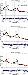 |
Fig. A.1. Analysis of C IV spectral region of SDSS spectra, as discussed in Section 2.1. Legend as in Figure 2. |
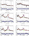 |
Fig. A.1. continued. |
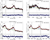 |
Fig. A.1. continued. |
Appendix B: Gallery of X-ray spectra
Figure B.1 presents the analysis of the Chandra X-ray data for our main dataset, as discussed in Section 3. To enhance visual clarity, the spectra in the plots are binned to ensure at least 1.5 counts per energy channel, except for SDSS J133610.96+184529.9, for which the spectrum in the plot is binned to ensure at least one count per energy channel. Black crosses represent the observational data with corresponding errors, red lines represent the best-fit models.
Appendix C: LX – LUV relation in redshift bins
The slope of the LX – LUV relation, when examined in redshift bins, does not show any clear trend with redshift (Lusso et al. 2020), yet slight statistical fluctuations are possible from bin to bin. Therefore, we additionally examine the X-ray intensity of the seven objects in our main dataset with Γ > 1.7 (i.e. those for which we can safely exclude significant X-ray absorption) in narrow redshift bins.
We determined the slope, intercept, and dispersion of the X-ray-to-UV luminosity relation for the subsets of the L20 sample within the redshift range z = 1.825 – 2.025 in bins with a step of Δz = 0.05. We utilised the same fitting method as for the complete L20 sample, namely the Python package EMCEE, conducting the regression fit with the normalisation of X-ray and UV luminosities set to the respective median values of the analysed subsets. We then supplemented the subsets of the L20 sample with the sources from our main dataset and repeated the fitting.
Figure C.1 displays the best-fit parameters (slope γ with its uncertainty and dispersion δ) of the LX – LUV relation obtained for the aforementioned subsamples. Objects from our main dataset are X-ray ‘normal’ within ΔC = 2.706 and the 2σ dispersion of the relation in their respective redshift bins. The addition of new sources maintains the same slope of the relation within the error margins for each analysed redshift interval. Meanwhile, the new sources occupy poorly populated areas of the plots, thereby improving the reliability of the fits.
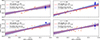 |
Fig. C.1. Rest-frame monochromatic luminosities LX against LUV in Δz = 0.05 redshift bins. Light red dots represent quasars from the Lusso et al. (2020) sample, with the relative regression lines shown in dashed red. Blue squares represent seven X-ray steep (Γ > 1.7) quasars in our main dataset, with the updated regression lines shown in dotted blue. |
All Tables
All Figures
|
Fig. 1. Shift of centroid of C IVλ1549 Å line in units of km/s, as function of logarithmic luminosity νLν at 2500 Å, available in Wu & Shen (2022). The sample consists of all the quasars in the SDSS DR16 sample with redshift in the z = 1.8–2.2 interval, colour-coded from red to black by the density of the underlying points. Empty cyan circles indicate 45 objects pre-selected for the one-by-one modelling of the C IV line with multiple components. Filled semi-transparent blue circles show a subset of 10 objects with the confirmed strongly blueshifted component, the main dataset analysed in this paper. Violet circles show four supplementary archival sources. |
| In the text | |
|
Fig. 2. Example of analysis of C IV spectral region of SDSS spectra. The fitted lines are reported as labels. The components employed in the fit are colour-coded, as shown in the legend. The reported C IV outflow velocity is measured as the shift of the outflow component with respect to the BLR component. The dashed vertical lines indicate the expected position for the fitted lines according to the redshift reported in the catalogue. The shaded light grey regions are telluric bands, narrow absorption lines, or bad pixels and are therefore excluded from the fit. See Appendix A for the analysis of other sources. |
| In the text | |
|
Fig. 3. C IV emission space with hexagons colour-coded by median He II EW for 66810 quasars in SDSS DR16 sample with redshift in z = 1.8 − 2.2 interval, having reliable C IV and He II measurements from MFICA reconstructions. Only hexagons with five or more quasars are plotted. Circles colour-coded by corresponding He II EW show the main dataset of 10 objects and four supplementary archival sources. |
| In the text | |
|
Fig. 4. Example of analysis of Chandra X-ray spectra. To enhance visual clarity, the spectrum in the plot is binned to ensure at least 1.5 counts per energy channel. Black crosses represent the observational data with corresponding errors, red line represents the best-fit model. See Appendix B for the analysis of other sources. |
| In the text | |
|
Fig. 5. Rest-frame monochromatic luminosities LX against LUV for 10 quasars in our main dataset and four additional quasars from Chandra and XMM-Newton archives, colour-coded by C IV outflow velocity in units of km/s, measured in our modelling of C IV line as the shift of the outflow component with respect to the BLR component. Colour-coded and empty black squares show modelling of J111800.50+195853.4 with a free and fixed photon index, respectively. Downward arrows indicate non-detection, and the corresponding squares represent upper limits. Light red dots represent the sample of about 2000 quasars from Lusso et al. (2020), with the relative regression line in red, for which the slope γ, with its error, and the dispersion δ are specified. The dashed and dotted lines trace the 1σ and 3σ dispersion, respectively. |
| In the text | |
|
Fig. A.1. Analysis of C IV spectral region of SDSS spectra, as discussed in Section 2.1. Legend as in Figure 2. |
| In the text | |
|
Fig. A.1. continued. |
| In the text | |
|
Fig. A.1. continued. |
| In the text | |
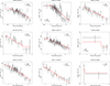 |
Fig. B.1. Analysis of Chandra X-ray spectra, as discussed in Section 3. Legend as in Figure 4. |
| In the text | |
|
Fig. C.1. Rest-frame monochromatic luminosities LX against LUV in Δz = 0.05 redshift bins. Light red dots represent quasars from the Lusso et al. (2020) sample, with the relative regression lines shown in dashed red. Blue squares represent seven X-ray steep (Γ > 1.7) quasars in our main dataset, with the updated regression lines shown in dotted blue. |
| In the text | |
Current usage metrics show cumulative count of Article Views (full-text article views including HTML views, PDF and ePub downloads, according to the available data) and Abstracts Views on Vision4Press platform.
Data correspond to usage on the plateform after 2015. The current usage metrics is available 48-96 hours after online publication and is updated daily on week days.
Initial download of the metrics may take a while.