| Issue |
A&A
Volume 707, March 2026
|
|
|---|---|---|
| Article Number | A227 | |
| Number of page(s) | 23 | |
| Section | Astronomical instrumentation | |
| DOI | https://doi.org/10.1051/0004-6361/202555859 | |
| Published online | 17 March 2026 | |
Euclid preparation
LXXVII. The NISP spectroscopy channel: Ground performance and calibration
1
Aix-Marseille Université, CNRS/IN2P3, CPPM,
Marseille,
France
2
Centre National d’Etudes Spatiales – Centre spatial de Toulouse,
18 avenue Edouard Belin,
31401
Toulouse Cedex 9,
France
3
Aix-Marseille Université, CNRS, CNES, LAM,
Marseille,
France
4
Max Planck Institute for Extraterrestrial Physics,
Giessenbachstr. 1,
85748
Garching,
Germany
5
Universitäts-Sternwarte München, Fakultät für Physik, Ludwig-Maximilians-Universität München,
Scheinerstrasse 1,
81679
München,
Germany
6
Max-Planck-Institut für Astronomie,
Königstuhl 17,
69117
Heidelberg,
Germany
7
INFN-Padova,
Via Marzolo 8,
35131
Padova,
Italy
8
Dipartimento di Fisica e Astronomia “G. Galilei”, Università di Padova,
Via Marzolo 8,
35131
Padova,
Italy
9
INAF-Osservatorio di Astrofisica e Scienza dello Spazio di Bologna,
Via Piero Gobetti 93/3,
40129
Bologna,
Italy
10
INAF-Osservatorio Astrofisico di Torino,
Via Osservatorio 20,
10025
Pino Torinese (TO),
Italy
11
Université Claude Bernard Lyon 1, CNRS/IN2P3, IP2I Lyon, UMR 5822,
Villeurbanne
69100,
France
12
INAF-Osservatorio Astronomico di Padova,
Via dell’Osservatorio 5,
35122
Padova,
Italy
13
Felix Hormuth Engineering,
Goethestr. 17,
69181
Leimen,
Germany
14
Institut de Física d’Altes Energies (IFAE), The Barcelona Institute of Science and Technology,
Campus UAB,
08193
Bellaterra (Barcelona),
Spain
15
Universidad Politécnica de Cartagena, Departamento de Electrónica y Tecnología de Computadoras,
Plaza del Hospital 1,
30202
Cartagena,
Spain
16
INFN-Bologna,
Via Irnerio 46,
40126
Bologna,
Italy
17
Institute of Space Sciences (ICE, CSIC), Campus UAB,
Carrer de Can Magrans, s/n,
08193
Barcelona,
Spain
18
Institut d’Estudis Espacials de Catalunya (IEEC), Edifici RDIT,
Campus UPC,
08860
Castelldefels, Barcelona,
Spain
19
Institute of Theoretical Astrophysics, University of Oslo,
PO Box 1029
Blindern,
0315
Oslo,
Norway
20
CEA-Saclay, DRF/IRFU, departement d’ingenierie des systemes,
bat472,
91191
Gif sur Yvette cedex,
France
21
Université Paris-Saclay, Université Paris Cité, CEA, CNRS, AIM,
91191
Gif-sur-Yvette,
France
22
Jet Propulsion Laboratory, California Institute of Technology,
4800 Oak Grove Drive,
Pasadena,
CA
91109,
USA
23
Technical University of Denmark,
Elektrovej 327,
2800 Kgs.
Lyngby,
Denmark
24
Cosmic Dawn Center (DAWN),
Denmark
25
NASA Goddard Space Flight Center,
Greenbelt,
MD
20771,
USA
26
ESAC/ESA, Camino Bajo del Castillo,
s/n., Urb. Villafranca del Castillo,
28692
Villanueva de la Cañada,
Madrid,
Spain
27
European Space Agency/ESTEC,
Keplerlaan 1,
2201 AZ
Noordwijk,
The Netherlands
28
Kapteyn Astronomical Institute, University of Groningen,
PO Box 800,
9700 AV
Groningen,
The Netherlands
29
SKA Observatory, Jodrell Bank, Lower Withington,
Macclesfield,
Cheshire
SK11 9FT,
UK
30
Institut d’Astrophysique de Paris,
98bis Boulevard Arago,
75014
Paris,
France
31
Institut d’Astrophysique de Paris, UMR 7095, CNRS, and Sorbonne Université,
98 bis boulevard Arago,
75014
Paris,
France
32
Space Science Data Center, Italian Space Agency,
via del Politecnico snc,
00133
Roma,
Italy
33
Leiden Observatory, Leiden University,
Einsteinweg 55,
2333 CC
Leiden,
The Netherlands
34
INFN-Sezione di Bologna,
Viale Berti Pichat 6/2,
40127
Bologna,
Italy
35
Carnegie Observatories,
Pasadena,
CA
91101,
USA
36
INAF-Osservatorio Astronomico di Brera,
Via Brera 28,
20122
Milano,
Italy
37
Infrared Processing and Analysis Center, California Institute of Technology,
Pasadena,
CA
91125,
USA
38
University of California,
Los Angeles,
CA
90095-1562,
USA
39
Port d’Informació Científica,
Campus UAB, C. Albareda s/n,
08193
Bellaterra (Barcelona),
Spain
40
Centro de Investigaciones Energéticas, Medioambientales y Tecnológicas (CIEMAT),
Avenida Complutense 40,
28040
Madrid,
Spain
41
Caltech/IPAC,
1200 E. California Blvd.,
Pasadena,
CA
91125,
USA
42
INAF-Osservatorio Astronomico di Trieste,
Via G. B. Tiepolo 11,
34143
Trieste,
Italy
43
INAF-IASF Milano,
Via Alfonso Corti 12,
20133
Milano,
Italy
44
Dipartimento di Fisica “Aldo Pontremoli”, Università degli Studi di Milano,
Via Celoria 16,
20133
Milano,
Italy
45
INFN-Sezione di Milano,
Via Celoria 16,
20133
Milano,
Italy
46
Centre de Calcul de l’IN2P3/CNRS,
21 avenue Pierre de Coubertin
69627
Villeurbanne Cedex,
France
47
Dipartimento di Fisica e Astronomia “Augusto Righi” – Alma Mater Studiorum Università di Bologna,
via Piero Gobetti 93/2,
40129
Bologna,
Italy
48
Waterloo Centre for Astrophysics, University of Waterloo,
Waterloo,
Ontario
N2L 3G1,
Canada
49
Department of Physics and Astronomy, University of Waterloo,
Waterloo,
Ontario
N2L 3G1,
Canada
50
Perimeter Institute for Theoretical Physics,
Waterloo,
Ontario
N2L 2Y5,
Canada
51
INAF-Osservatorio Astronomico di Roma,
Via Frascati 33,
00078
Monteporzio Catone,
Italy
52
INFN-Sezione di Roma,
Piazzale Aldo Moro 2, c/o Dipartimento di Fisica, Edificio G. Marconi,
00185
Roma,
Italy
53
California Institute of Technology,
1200 E California Blvd,
Pasadena,
CA
91125,
USA
54
Université Paris-Saclay, CNRS, Institut d’astrophysique spatiale,
91405
Orsay,
France
55
School of Mathematics and Physics, University of Surrey,
Guildford,
Surrey
GU2 7XH,
UK
56
IFPU, Institute for Fundamental Physics of the Universe,
via Beirut 2,
34151
Trieste,
Italy
57
INFN, Sezione di Trieste,
Via Valerio 2,
34127
Trieste TS,
Italy
58
SISSA, International School for Advanced Studies,
Via Bonomea 265,
34136
Trieste TS,
Italy
59
Dipartimento di Fisica e Astronomia, Università di Bologna,
Via Gobetti 93/2,
40129
Bologna,
Italy
60
Dipartimento di Fisica, Università di Genova,
Via Dodecaneso 33,
16146
Genova,
Italy
61
INFN-Sezione di Genova,
Via Dodecaneso 33,
16146
Genova,
Italy
62
Department of Physics “E. Pancini”, University Federico II,
Via Cinthia 6,
80126
Napoli,
Italy
63
INAF-Osservatorio Astronomico di Capodimonte,
Via Moiariello 16,
80131
Napoli,
Italy
64
Instituto de Astrofísica e Ciências do Espaço, Universidade do Porto, CAUP, Rua das Estrelas,
4150-762
Porto,
Portugal
65
Faculdade de Ciências da Universidade do Porto, Rua do Campo de Alegre,
4150-007
Porto,
Portugal
66
Dipartimento di Fisica, Università degli Studi di Torino,
Via P. Giuria 1,
10125
Torino,
Italy
67
INFN-Sezione di Torino,
Via P. Giuria 1,
10125
Torino,
Italy
68
Institute Lorentz, Leiden University,
Niels Bohrweg 2,
2333 CA
Leiden,
The Netherlands
69
Institute for Theoretical Particle Physics and Cosmology (TTK), RWTH Aachen University,
52056
Aachen,
Germany
70
INFN section of Naples,
Via Cinthia 6,
80126,
Napoli,
Italy
71
Institute for Astronomy, University of Hawaii,
2680 Woodlawn Drive,
Honolulu,
HI
96822,
USA
72
Dipartimento di Fisica e Astronomia “Augusto Righi” – Alma Mater Studiorum Università di Bologna,
Viale Berti Pichat 6/2,
40127
Bologna,
Italy
73
Instituto de Astrofísica de Canarias,
Vía Láctea,
38205
La Laguna,
Tenerife,
Spain
74
Institute for Astronomy, University of Edinburgh, Royal Observatory,
Blackford Hill,
Edinburgh
EH9 3HJ,
UK
75
Jodrell Bank Centre for Astrophysics, Department of Physics and Astronomy, University of Manchester,
Oxford Road,
Manchester
M13 9PL,
UK
76
European Space Agency/ESRIN,
Largo Galileo Galilei 1,
00044
Frascati,
Roma,
Italy
77
Institut de Ciències del Cosmos (ICCUB), Universitat de Barcelona (IEEC-UB),
Martí i Franquès 1,
08028
Barcelona,
Spain
78
Institució Catalana de Recerca i Estudis Avançats (ICREA),
Passeig de Lluís Companys 23,
08010
Barcelona,
Spain
79
UCB Lyon 1, CNRS/IN2P3, IUF, IP2I Lyon,
4 rue Enrico Fermi,
69622
Villeurbanne,
France
80
Canada–France–Hawaii Telescope,
65-1238 Mamalahoa Hwy,
Kamuela,
HI
96743,
USA
81
Departamento de Física, Faculdade de Ciências, Universidade de Lisboa,
Edifício C8, Campo Grande,
1749-016
Lisboa,
Portugal
82
Instituto de Astrofísica e Ciências do Espaço, Faculdade de Ciências, Universidade de Lisboa,
Campo Grande,
1749-016
Lisboa,
Portugal
83
Department of Astronomy, University of Geneva,
ch. d’Ecogia 16,
1290
Versoix,
Switzerland
84
INAF-Istituto di Astrofisica e Planetologia Spaziali,
via del Fosso del Cavaliere, 100,
00100
Roma,
Italy
85
School of Physics, HH Wills Physics Laboratory, University of Bristol,
Tyndall Avenue,
Bristol,
BS8 1TL,
UK
86
FRACTAL S.L.N.E.,
calle Tulipán 2, Portal 13 1A,
28231,
Las Rozas de Madrid,
Spain
87
Department of Physics, Lancaster University,
Lancaster
LA1 4YB,
UK
88
Department of Physics and Helsinki Institute of Physics,
Gustaf Hällströmin katu 2,
00014
University of Helsinki,
Finland
89
Université de Genève, Département de Physique Théorique and Centre for Astroparticle Physics,
24 quai Ernest-Ansermet,
1211
Genève 4,
Switzerland
90
Department of Physics,
PO Box 64,
00014
University of Helsinki,
Finland
91
Helsinki Institute of Physics, Gustaf Hällströmin katu 2, University of Helsinki,
Helsinki,
Finland
92
Laboratoire d’etude de l’Univers et des phenomenes eXtremes, Observatoire de Paris, Université PSL, Sorbonne Université, CNRS,
92190
Meudon,
France
93
Mullard Space Science Laboratory, University College London,
Holmbury St Mary, Dorking,
Surrey
RH5 6NT,
UK
94
University of Applied Sciences and Arts of Northwestern Switzerland, School of Computer Science,
5210
Windisch,
Switzerland
95
Universität Bonn, Argelander-Institut für Astronomie,
Auf dem Hügel 71,
53121
Bonn,
Germany
96
Department of Physics, Institute for Computational Cosmology, Durham University,
South Road,
Durham
DH1 3LE,
UK
97
Université Côte d’Azur, Observatoire de la Côte d’Azur, CNRS, Laboratoire Lagrange,
Bd de l’Observatoire,
CS 34229,
06304
Nice cedex 4,
France
98
Université Paris Cité, CNRS, Astroparticule et Cosmologie,
75013
Paris,
France
99
CNRS-UCB International Research Laboratory, Centre Pierre Binétruy,
IRL2007,
CPB-IN2P3,
Berkeley,
USA
100
University of Applied Sciences and Arts of Northwestern Switzerland, School of Engineering,
5210
Windisch,
Switzerland
101
Institute of Physics, Laboratory of Astrophysics, Ecole Polytechnique Fédérale de Lausanne (EPFL),
Observatoire de Sauverny,
1290
Versoix,
Switzerland
102
Aurora Technology for European Space Agency (ESA),
Camino bajo del Castillo, s/n, Urbanizacion Villafranca del Castillo, Villanueva de la Cañada,
28692
Madrid,
Spain
103
School of Mathematics, Statistics and Physics, Newcastle University,
Herschel Building,
Newcastle-upon-Tyne
NE1 7RU,
UK
104
DARK, Niels Bohr Institute, University of Copenhagen,
Jagtvej 155,
2200
Copenhagen,
Denmark
105
Institute of Space Science,
Str. Atomistilor, nr. 409 Măgurele,
Ilfov,
077125,
Romania
106
Consejo Superior de Investigaciones Cientificas,
Calle Serrano 117,
28006
Madrid,
Spain
107
Universidad de La Laguna, Departamento de Astrofísica,
38206
La Laguna, Tenerife,
Spain
108
Institut für Theoretische Physik, University of Heidelberg,
Philosophenweg 16,
69120
Heidelberg,
Germany
109
Institut de Recherche en Astrophysique et Planétologie (IRAP), Université de Toulouse, CNRS, UPS, CNES,
14 Av. Edouard Belin,
31400
Toulouse,
France
110
Université St Joseph, Faculty of Sciences,
Beirut,
Lebanon
111
Departamento de Física, FCFM, Universidad de Chile,
Blanco Encalada
2008,
Santiago,
Chile
112
Universität Innsbruck, Institut für Astro- und Teilchenphysik,
Technikerstr. 25/8,
6020
Innsbruck,
Austria
113
Instituto de Astrofísica e Ciências do Espaço, Faculdade de Ciências, Universidade de Lisboa,
Tapada da Ajuda,
1349-018
Lisboa,
Portugal
114
Cosmic Dawn Center (DAWN)
115
Niels Bohr Institute, University of Copenhagen,
Jagtvej 128,
2200
Copenhagen,
Denmark
116
Dipartimento di Fisica e Scienze della Terra, Università degli Studi di Ferrara,
Via Giuseppe Saragat 1,
44122
Ferrara,
Italy
117
Istituto Nazionale di Fisica Nucleare, Sezione di Ferrara,
Via Giuseppe Saragat 1,
44122
Ferrara,
Italy
118
INAF, Istituto di Radioastronomia,
Via Piero Gobetti 101,
40129
Bologna,
Italy
119
Department of Physics, Oxford University,
Keble Road,
Oxford
OX1 3RH,
UK
120
INAF – Osservatorio Astronomico di Brera,
via Emilio Bianchi 46,
23807
Merate,
Italy
121
INAF – Osservatorio Astronomico di Brera, Via Brera 28, 20122 Milano, Italy, and INFN-Sezione di Genova,
Via Dodecaneso 33,
16146
Genova,
Italy
122
ICL, Junia, Université Catholique de Lille, LITL,
59000
Lille,
France
123
ICSC – Centro Nazionale di Ricerca in High Performance Computing, Big Data e Quantum Computing,
Via Magnanelli 2,
Bologna,
Italy
124
Instituto de Física Teórica UAM-CSIC,
Campus de Cantoblanco,
28049
Madrid,
Spain
125
CERCA/ISO, Department of Physics, Case Western Reserve University,
10900 Euclid Avenue,
Cleveland,
OH
44106,
USA
126
Technical University of Munich, TUM School of Natural Sciences, Physics Department,
James-Franck-Str. 1,
85748
Garching,
Germany
127
Max-Planck-Institut für Astrophysik,
Karl-Schwarzschild-Str. 1,
85748
Garching,
Germany
128
Laboratoire Univers et Théorie, Observatoire de Paris, Université PSL, Université Paris Cité, CNRS,
92190
Meudon,
France
129
Departamento de Física Fundamental. Universidad de Salamanca. Plaza de la Merced s/n,
37008
Salamanca,
Spain
130
Université de Strasbourg, CNRS, Observatoire astronomique de Strasbourg, UMR 7550,
67000
Strasbourg,
France
131
Center for Data-Driven Discovery, Kavli IPMU (WPI), UTIAS, The University of Tokyo,
Kashiwa,
Chiba
277-8583,
Japan
132
Dipartimento di Fisica – Sezione di Astronomia, Università di Trieste,
Via Tiepolo 11,
34131
Trieste,
Italy
133
Department of Physics & Astronomy, University of California Irvine,
Irvine,
CA
92697,
USA
134
Department of Mathematics and Physics E. De Giorgi, University of Salento,
Via per Arnesano,
CP-I93,
73100
Lecce,
Italy
135
INFN, Sezione di Lecce,
Via per Arnesano,
CP-193,
73100
Lecce,
Italy
136
INAF-Sezione di Lecce,
c/o Dipartimento Matematica e Fisica, Via per Arnesano,
73100
Lecce,
Italy
137
Departamento Física Aplicada, Universidad Politécnica de Cartagena,
Campus Muralla del Mar,
30202
Cartagena, Murcia,
Spain
138
Instituto de Física de Cantabria,
Edificio Juan Jordá, Avenida de los Castros,
39005
Santander,
Spain
139
Observatorio Nacional, Rua General Jose Cristino,
77-Bairro Imperial de Sao Cristovao,
Rio de Janeiro
20921-400,
Brazil
140
CEA Saclay, DFR/IRFU, Service d’Astrophysique,
Bat. 709,
91191
Gif-sur-Yvette,
France
141
Institute of Cosmology and Gravitation, University of Portsmouth,
Portsmouth
PO1 3FX,
UK
142
Department of Computer Science, Aalto University,
PO Box 15400,
Espoo
00 076,
Finland
143
Instituto de Astrofísica de Canarias, c/ Via Lactea s/n, La Laguna 38200, Spain. Departamento de Astrofísica de la Universidad de La Laguna,
Avda. Francisco Sanchez,
La Laguna
38200,
Spain
144
Ruhr University Bochum, Faculty of Physics and Astronomy, Astronomical Institute (AIRUB), German Centre for Cosmological Lensing (GCCL),
44780
Bochum,
Germany
145
Department of Physics and Astronomy,
Vesilinnantie 5,
20014
University of Turku,
Finland
146
Serco for European Space Agency (ESA),
Camino bajo del Castillo, s/n, Urbanizacion Villafranca del Castillo, Villanueva de la Cañada,
28692
Madrid,
Spain
147
ARC Centre of Excellence for Dark Matter Particle Physics,
Melbourne,
Australia
148
Centre for Astrophysics & Supercomputing, Swinburne University of Technology,
Hawthorn,
Victoria
3122,
Australia
149
Department of Physics and Astronomy, University of the Western Cape,
Bellville,
Cape Town,
7535,
South Africa
150
DAMTP, Centre for Mathematical Sciences,
Wilberforce Road,
Cambridge
CB3 0WA,
UK
151
Kavli Institute for Cosmology Cambridge,
Madingley Road,
Cambridge,
CB3 0HA,
UK
152
Department of Astrophysics, University of Zurich,
Winterthurerstrasse 190,
8057
Zurich,
Switzerland
153
Department of Physics, Centre for Extragalactic Astronomy, Durham University,
South Road,
Durham
DH1 3LE,
UK
154
IRFU, CEA, Université Paris-Saclay
91191
Gif-sur-Yvette Cedex,
France
155
Oskar Klein Centre for Cosmoparticle Physics, Department of Physics, Stockholm University,
Stockholm
106 91,
Sweden
156
Astrophysics Group, Blackett Laboratory, Imperial College London,
London
SW7 2AZ,
UK
157
Univ. Grenoble Alpes, CNRS, Grenoble INP, LPSC-IN2P3,
53, Avenue des Martyrs,
38000
Grenoble,
France
158
INAF-Osservatorio Astrofisico di Arcetri,
Largo E. Fermi 5,
50125
Firenze,
Italy
159
Dipartimento di Fisica, Sapienza Università di Roma,
Piazzale Aldo Moro 2,
00185
Roma,
Italy
160
Centro de Astrofísica da Universidade do Porto,
Rua das Estrelas,
4150-762
Porto,
Portugal
161
HE Space for European Space Agency (ESA),
Camino bajo del Castillo, s/n, Urbanizacion Villafranca del Castillo, Villanueva de la Cañada,
28692
Madrid,
Spain
162
Department of Astrophysical Sciences, Peyton Hall, Princeton University,
Princeton,
NJ
08544,
USA
163
Theoretical astrophysics, Department of Physics and Astronomy, Uppsala University,
Box 516,
751 37
Uppsala,
Sweden
164
Mathematical Institute, University of Leiden,
Einsteinweg 55,
2333 CA
Leiden,
The Netherlands
165
Institute of Astronomy, University of Cambridge,
Madingley Road,
Cambridge
CB3 0HA,
UK
166
Space physics and astronomy research unit, University of Oulu,
Pentti Kaiteran katu 1,
90014
Oulu,
Finland
167
Center for Computational Astrophysics, Flatiron Institute,
162 5th Avenue,
New York,
NY
10010,
USA
★ Corresponding author: This email address is being protected from spambots. You need JavaScript enabled to view it.
Received:
7
June
2025
Accepted:
15
September
2025
Abstract
ESA’s Euclid cosmology mission relies on the very sensitive and accurately calibrated spectroscopy channel of the Near-Infrared Spectrometer and Photometer (NISP). With three operational grisms in two wavelength intervals, NISP provides diffraction-limited slitless spectroscopy over a field of 0.57 deg2. A blue grism, BGE, covers the wavelength range 926–1366 nm at a spectral resolution (ℛ) of 440–900 for a 0.″5 diameter source with a dispersion of 1.24 nm px−1. Two red grisms, RGE, span 1206 to 1892 nm at ℛ = 550–740 and a dispersion of 1.37 nm px−1. We describe the construction of the grisms as well as the ground testing of the flight model of the NISP instrument, where these properties were established.
Key words: instrumentation: spectrographs / space vehicles: instruments / techniques: imaging spectroscopy / techniques: spectroscopic / cosmology: observations
Publisher note: The article number in this series contained a typo. The Roman numeral in the subtitle was corrected on 25 March 2026.
© The Authors 2026
 Open Access article, published by EDP Sciences, under the terms of the Creative Commons Attribution License (https://creativecommons.org/licenses/by/4.0), which permits unrestricted use, distribution, and reproduction in any medium, provided the original work is properly cited.
This article is published in open access under the Subscribe to Open model. This email address is being protected from spambots. You need JavaScript enabled to view it. to support open access publication.
1 Introduction
Euclid is a new space mission within the European Space Agency’s (ESA) Cosmic Vision 2015–2025 programme; its goal is to study the nature of dark matter and dark energy by estimating the expansion history of the Universe and the growth rate of cosmic structures (Laureijs et al. 2011; Euclid Collaboration: Mellier et al. 2025). For this purpose Euclid was designed as a wide-field telescope in the visible to near-infrared (NIR) wavelength range to survey ∼14 000 deg2 of extragalactic sky from the Sun–Earth Lagrange point 2 (Euclid Collaboration: Scaramella et al. 2022).
Euclid’s payload consists of two scientific instruments developed by the Euclid Consortium: VIS provides high-resolution images of the sky in a single broad wavelength band from 550 nm to 950 nm (Euclid Collaboration: Cropper et al. 2025). With a spatial sampling of 0.″1 and a tight control on the point spread function (PSF), the VIS instrument is optimised for the measurement of galaxy shapes for weak lensing, which enables the mapping of dark matter structure as a tool for cosmological studies (Cropper et al. 2016; Euclid Collaboration: Cropper et al. 2025). Euclid’s second instrument, the Near-Infrared Spectrometer and Photometer (NISP) (Euclid Collaboration: Jahnke et al. 2025), operates in the NIR and shares a common field of view (FoV) of 0.54 deg2 with VIS (Euclid Collaboration: Mellier et al. 2025) thanks to a dichroic transparent to NIR that is located in front of the NISP entrance pupil. NISP has been designed to take spectroscopic measurements of galaxy distances in order to probe galaxy clustering, as well as to obtain NIR information to be used to determine photometric redshifts.
As a cosmology mission, Euclid’s ultimate goal is to reach a combined cosmological figure of merit (FoM) of ≥400 (Euclid Collaboration: Mellier et al. 2025) on the dark energy parameters (wp, wa) with weak lensing and galaxy clustering. Reaching this ambitious goal requires a combined approach that leverages both a comprehensive joint analysis of weak gravitational lensing, galaxy-galaxy lensing, and galaxy clustering (commonly referred to as a 3 × 2-point analysis) and a 3D galaxy clustering analysis using spectroscopic redshifts to evaluate cosmological distances. To that end, the Euclid spectroscopic survey is designed to target Hα line-emitting galaxies in the redshift range 0.9–1.8, thereby providing precise measurements of the growth of structure and redshift-space distortions as well as the expansion history via baryon acoustic oscillations. Consequently, the galaxy clustering analyses require spectroscopic redshifts (z) to be obtained for at least 1700 galaxies per square degree. This corresponds to redshift measurements for ∼2.55×10⁷ galaxies over the survey area of ∼14 000 deg2 of the Euclid Wide Survey (Euclid Collaboration: Scaramella et al. 2022) achieved through slitless spectroscopy. The Euclid core science also requires the galaxy redshifts to be estimated with an accuracy (σz) of ≤ 0.001(1 + z), which translates to a minimal spectral resolution (λ/∆λ) of ≥ 380 when considering a source size of 0.″5.
This work focuses on evaluating NISP spectroscopic performance through the analysis of PSF quality and spectral dispersion properties. In the following we describe the NISP spectroscopic channel that was designed and built for Euclid’s NIR spectroscopic survey. Section 2 provides a general overview of the NISP instrument as well as the grisms, which are the key components for NISP’s spectroscopic capabilities. The setup for NISP ground tests of the spectroscopic channel are described in Sect. 3. NISP’s spectroscopic optical quality is presented in Sect. 4, and Sect. 5 presents a detailed analysis of the grisms’ dispersion properties. In Sect. 6 the overall resulting spectroscopic performance is discussed. The paper closes with a brief conclusion and a description of available data products characterising the grisms in Sect. 7.
2 The NISP instrument
The NISP instrument (Maciaszek et al. 2022; Euclid Collaboration: Jahnke et al. 2025) is a NIR spectrometer and photometer whose spectroscopic channel has been designed and optimised to detect Hα emission line galaxies in the redshift range z ∈ [0.9, 1.8]. The NISP general layout and components are shown in Fig. 1 – a full presentation of the instrument can be found in Euclid Collaboration: Jahnke et al. (2025), and the photometry channel and bandpasses are described in Euclid Collaboration: Schirmer et al. (2022). Here we provide a brief introduction into the central aspects relevant for spectroscopy.
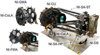 |
Fig. 1 Schematic view of the NISP instrument detailing its subsystems. Right: view of the whole instrument as integrated. Left: detailed view with an open wheel cavity, showing the locations of the two wheels to select spectral elements. Not shown are the ‘warm’ electronics, which are used for commands and data processing; they are located away from the main NISP instrument assembly in Euclid’s service module (Maciaszek et al. 2016). The subsystem names and functions are described in the main text. |
2.1 Overview of NISP components and properties
NISP consists of a silicon carbide (SiC) mechanical structure (NISP Structure Assembly STructure – NI-SA-ST) that houses the detector system (NI-DS) on one side and the optical system on the other (Bougoin et al. 2017). The SiC was chosen for its stiffness and its thermal stability, which allows optical alignment and stability to be maintained over the mission lifetime. Additionally, fine tuning of internal NISP heaters maintain the opto-mechanics temperature in the required range around 135 K–140 K to further maintain optical alignment. Low conductance (0.043 W K−1 in total) bipods and monopod (NISP Structure Assembly HexaPods – NI-SA-HP) interface the NISP instrument with the Euclid payload module (PLM) baseplate.
The NI-DS (Bonnefoi et al. 2016) acquires images by sampling the FoV with 16 HgCdTe 2k × 2k pixels NIR detectors produced by Teledyne Imaging Sensors, arranged in a 4 × 4 mosaic. Their pixel size of 18 µm provides NISP with a spatial sampling of the sky of 0.″3 px−1, and the detectors have their wavelength cut-off tuned to 2.3 µm to minimise thermal noise from the optical system’s thermal emission. Maintaining the focal plane below 95 K is crucial for optimal performance and is achieved through thermal coupling of the instrument with an external radiator using four highly conductive thermal straps. Furthermore, NISP’s detectors are read out by 16 individual SIDECAR ASICs, each operating at approximately 140 K and dissipating up to 4.8 W of heat. To manage this heat load effectively, high-efficiency thermal coupling to the baseplate is employed, facilitated by methane heat pipes (MHP). Due to the substantial heat dissipation, a large radiator of approximately 2 m2 is required to radiate this heat into space, accounting for both the electronics’ heat and any conductive or radiative leaks between the PLM and the radiator.
The NISP instrument images the sky in two different channels: a photometric channel for the acquisition of images with broadband filters and a spectrometric channel for the acquisition of slitless dispersed images. The optical system of NISP (Bodendorf et al. 2019; Grupp et al. 2012) comprises several elements; a spherical-aspherical meniscus-type corrector lens (CoLA) at the entrance of NISP that actively takes part in correcting the chromatic aberration of the image; the filter wheel (NI-FWA) with a set of three filters (Euclid Collaboration: Schirmer et al. 2022), namely YE (950–1212 nm), JE (1168– 1567 nm) and HE (1522–2021 nm) as well as a ‘closed’ position, blocking light from the telescope; the grism wheel (NI-GWA) with a set of three red grisms (1206−1892 nm), a single blue grism (926–1366 nm), and an open position; and finally an assembly of three lenses, which, together with their holding structure, constitute the camera lens assembly (CaLA), focusing light onto the detector plane.
2.2 The NISP grisms
The key components in creating dispersed light for determining redshifts of distant galaxies are the NISP grisms. They are the combination of a transmission grating with a prism. This combination allowed us to create a common FoV with the NISP photometry channel, placing the dispersed light onto the same detector plane. The NISP instrument contains four different grisms, RGS000, RGS180, RGS270, and BGS000, three in a red and one in a blue bandpass.
Each of the grisms comprises several optical elements, each fulfilling a specific function (Costille et al. 2019), presented in Fig. 2. A resin-free blazed dispersion grating (dark blue) is directly engraved onto the hypotenuse surface of a fused-silica prism (light blue) to disperse the light. Each grism has a diameter of 140 mm and a central thickness of approximately 12 mm (Costille et al. 2014), making them the largest grisms ever flown into space. The prism and the grating design were defined to maximise transmission efficiency at the un-deflected wavelength of about 1.2 µm for the red and 0.9 µm for the blue grisms, with transmission required to be higher than 70% in grism bandpass. Additionally, the grating groove has been engraved with a curvature on the hypotenuse surface of the prism to apply a spectral wavefront correction to the incoming light. The base of the prism carries optical power, that is, it has a curved surface (dashed line) to provide a fine-focus correction for the incoming light beam towards the NISP detection plane. Finally, a multi-layer coating (yellow) has been deposited on the curved surface to define each grism’s transmission bandpass.
The grisms RGS000, RGS180, and RGS270 are three red grisms transmitting light in the ‘red’ spectroscopic bandpass (RGE) wich range from about 1206 nm to 1892 nm, with these wavelengths marking half of the maximum of the in-band transmission. The grism BGS000 is a blue grism with a spectral band ranging from about 880 nm to 1366 nm. Combined with the transmission characteristics of Euclid’s dichroic and telescope mirrors, the Euclid ‘blue’ spectroscopic bandpass (BGE) is reduced to 926–1366 nm. This work focuses on the grism characteristics themselves, as telescope mirrors and dichroic were not present during the instrument test campaigns. Their – well-known – characteristics are simply folded in later.
The grisms create different orientations of spectral dispersion on the focal plane. With a view from the NISP optics towards the projected spectra on the detector plane and with grism RGS000 as the reference, the grism RGS180 has a 180◦ orientation and hence disperses light in the opposite direction to RGS000. Similarly, RGS270 has a 270◦ counter-clockwise orientation with respect to RGS000. These three different orientations were chosen to permit the ‘decontamination’ of spectra from overlaps with other sources, creating a reconstructed spectrum from successively acquired exposures of a given field with the three red grisms.
Each grism is glued onto six Invar pads, whose coefficient of thermal expansion closely matches silica. The blades are bonded to flexible aluminium-alloy blades that limit stress transmission during the cooldown; these blades are part of the aluminium-alloy mount, which is directly integrated into the grism wheel (Riva et al. 2011).
 |
Fig. 2 Cross-section of a NISP grisms. The prism wedge (light blue) has an added curved basis surface onto which the filter coating is deposited (yellow), while the grooves of the dispersion grating (dark blue) are directly engraved onto the flat hypotenuse surface of the prism. The grisms are characterised by their prism angle (A), the groove height (H), and the blaze angle (β). |
3 NISP ground testing setup
After completion of the instrument integration in 2019, the NISP flight model underwent a series of tests in vacuum and with the instrument cooled down to its operational temperature. Two test campaigns were conducted inside the ERIOS vacuum chamber at the Laboratoire d’Astrophysique de Marseille (LAM) in the fall of 2019 and the beginning of 2020, to validate the instrument’s performance and its functionality in a space environment. The ERIOS chamber (Costille et al. 2016b) is a large cryogenic chamber, with an external envelope of 6 m in length and a diameter of 4 m, capable of achieving high vacuum (∼10−6 mbar) and to cool down an inner volume of 45 m3 to low temperatures (∼80 K) with a high stability (±4 mK) thanks to liquid nitrogen shrouds covering the entire inner surface of the chamber.
In addition, various types of ground-support equipment were specifically developed by the NISP instrument team to enable the ground tests (Costille et al. 2017). One important component was a point-like light source developed to measure the NISP object plane and to verify NISP’s optical performance, mainly plate scale across the detector plane, point-spread-function width, and a rough estimate of ghost images. The point-like source was the combination of a pinhole light source and a telescope made of a 160 mm diameter elliptical off-axis mirror with primary and secondary focal points at 500 mm and 3000 mm, respectively, simulating Euclid’s F/20 telescope beam.
The entire aperture of the mirror was illuminated through this 2 µm pinhole located at the primary focus of the elliptical mirror, creating a point source for NISP. The mirror and the pinhole were both attached to the same baseplate and the whole system (mirror, pinhole, and baseplate) was made from silica to ensure stability of the mirror’s focal distance. The telescope baseplate was attached to translation and rotation stages using thermal flexures made from a low conductivity material, thermally isolating the telescope, while providing it with 5 degrees of freedom when being pointed towards different positions in NISP’s FoV.
During the tests, this telescope was inside the ERIOS chamber, together with the instrument, and was operated at temperature of ≃160 K with stability of 0.04 K over a test duration of 1 month. The motors of the telescope mount were kept at warm ambient temperature and were isolated from the cold environment of the ERIOS chamber by a multi-layer insulation blanket.
Inside ERIOS, light was fed to the telescope through a cryogenic fibre connected to the pinhole, with light sources being located outside the chamber. At the interface of the ERIOS chamber a pair of vacuum windows connected the fibre with the light sources, using a cooled neutral density filter to suppress thermal background. On the outside, a set of neutral density filters allowed us to select the intensity of light entering the fibre.
Different types of light sources were used during the instrument test campaigns. Among them was a continuum laser source that was connected either to a monochromator, providing a selectable monochromatic wavelength in the range from 0.4 µm to 2.1 µm, or to a Fabry–Pérot etalon to emulate an emission-line spectrum with a total of 64 emission lines in the bandpass of the NISP grisms. Alternatively, an argon lamp could be used as a source to provide a well-known reference spectrum for comparison with the Fabry–Pérot etalon. The monochromator and the Fabry–Pérot etalon were both characterised before delivery to the ground test equipment.
Spectral lamps were fed into the monochromator to characterise and calibrate it, using HgCd, He, or Cs lamps for the visible band below 1.1 μm, and an Ar lamp for the NIR domain. The output of the monochromator was scanned using either silicon or germanium photodiodes. The calibration yielded a selectable maximum wavelength accuracy of 0.4 nm, and the full width at half maximum (FWHM) of the monochromator bandwidth was measured to be approximately 0.41 nm.
The etalon was re-aligned and re-calibrated in warm conditions with a Perkin Elmer Lambda 900 UV/VIS/NIR spectrometer (‘Lambda 900’) before testing of NISP started. During the tests, thermal sensor monitored the stability of the light sources and the etalon. Figure 3 shows the Fabry–Pérot etalon’s spectrum as it was measured and calibrated with a 1σ precision of ±0.2 nm using the Lambda 900 spectrometer. A comparison to the grisms’ transmission shows the number of Fabry–Pérot’s peaks available for calibration. The grism channels’ total transmission shown here accounts for the transmission of the CoLA and CaLA lenses, the grisms themselves, as well as the detector quantum efficiency. In this figure neither the Euclid mirrors nor dichroic are accounted for, as neither element was present in the instrument-level test setup. Note that in Fig. 3 the transmission of the zeroth-order components of NISP’s spectrograms, which are below a few per cent at maximum, have been multiplied by a factor of 10 to make them stand out. Additionally, the optical transmission shown in Fig. 3 is derived from combined subsystem-level measurements. Due to limited knowledge of the optical ground equipment transmission – including fibre, pinhole, and telescope contribution to the total transmission – and the absence of a calibrated photodiode in the ERIOS chamber, we were unable to measure the absolute transmission of the NISP optics during the ground test campaign, and thus we relied on subsystem measurements to estimate the total transmission presented in Fig. 3.
Prior to the start of the optical tests, the focal length of the NISP instrument was measured at cold (NISP focal plane at ≃85 K and NISP optics at ≃135 K), using a monochromatic light beam with a wavelength of 1000 nm in the YE photometric passband. In this process, PSF widths were measured from spots created by the point source. This was carried out at five positions in the NISP FoV, where hundreds of individual slightly dithered exposures were taken to over-sample the PSF and to increase statistical accuracy on the PSF width measurement. This was repeated for different distances of the telescope simulator from NISP. During the PSF acquisitions, the relative distance between NISP and the telescope simulator was accurately monitored with a laser tracker system that measured the position of ten targets attached to the NISP mechanical structure relative to five targets attached to the back of the telescope mirror (Costille et al. 2016a, 2018).
This set of measurements provided a reference focal plane position for the instrument in the YE passband. From these measurements an optimal object plane position was identified, using an as-built Zemax model1 (Moore et al. 2004) of the NISP instrument, providing the best image quality in all NISP filter and grism bandpasses. All subsequent instrument tests where then made with the telescope simulator pinhole positioned on this optimal object plane.
It is important to note that this measurement also established the fixed reference plane for positioning NISP relative to the VIS instrument, ensuring optimal NISP image quality once the Euclid telescope is focused on the VIS instrument, which has more stringent image quality requirements. The relative alignment between NISP and VIS was verified during the PLM ground tests and is beyond the scope of this paper. Nevertheless, the excellent optical performance delivered by NISP in flight confirms the accuracy and stability of its alignment with the Euclid telescope.
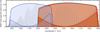 |
Fig. 3 Total transmission of the spectra’s first order (solid line) and ten times total transmission of the spectra’s zeroth order (dashed line) for the BGS000 (blue), RGS000 (light red), RGS180 (orange), and RGS270 (dark red) grism channels. The total transmission accounts for the transmission of the grisms themselves, of CoLA and CaLA, and includes the detector quantum efficiency. For comparison, the Fabry–Pérot etalon spectrum (light grey) is shown as measured in the laboratory with a Lambda 900 spectrometer, in arbitrary data units. The contributions from neither the dichroic nor telescope are accounted for in these measurements as Euclid mirrors as well as its dichroic were not emulated during the instrument tests. |
4 NISP spectroscopic optical quality
This section describes the optical quality of the NISP spectroscopic channel, when a grism is moved into the NISP science beam. First, RGS000, RGS180, and BGS000 are discussed, then the special case of RGS270, for which a non-conformance has been identified during instrument tests, rendering it in-operational for science use.
4.1 Optical quality of RGS000, RGS180, and BGS000
The NISP optical quality was assessed by evaluating the radii that encircle 50% and 80% of the PSF’s total energy – in the following these radii are referred to as EE50 and EE80, respectively. In the spectroscopic channel, this verification was done for every grism of the NI-FWA at three monochromatic wavelengths: 1300 nm, 1500 nm, and 1800 nm for all three red grisms and 900 nm, 1120 nm, and 1340 nm for the blue grism. Additionally, we tested image quality of both RGS000 and RGS180 with a ±4◦ grism wheel rotation offset to validate that offsetting the grism positions by this amount would not degrade image quality. This additional measurement was part of an evaluation of a modified survey strategy to overcome the reduced quality of data from RGS270 (see Sect. 4.2).
The image quality was evaluated with an analysis of monochromatic PSF images taken at the four corners of the NISP FoV. Because the NISP plate scale of 0.″3 per pixel under-samples the PSF, hundreds of PSF images were acquired around each position, dithering by a tenth of a pixel around the target position in the NISP image plane. This dithering, obtained by moving the telescope on its axes, allowed us to spatially over-sample the PSFs and reduced the statistical uncertainties on the EE50 and EE80 measurements.
Before measuring PSF properties, images acquired by the NISP instrument were corrected for pixel quantum efficiency and conversion gain, and a NISP residual thermal background acquired under ‘dark test conditions’, i.e. with the NISP NI-FWA in closed position and all light sources turned off. An automatic procedure, derived from the work of Jiang et al. (2016), was used to locate the PSF within the 2k × 2k pixels of the target detectors. Once located, a 20 × 20 pixel stamp centred on the expected PSF position was extracted from the images and PSF metrics were extracted by image analyses. Every extracted sub-image was controlled by eye, and, for example, detector cosmetic defects misidentified as PSFs by our algorithm were rejected from the analyses. An intra-pixel capacitance (IPC) correction, relying on a Richardson–Lucy deconvolution method (Lucy 1974; Richardson 1972) using IPC coefficients previously measured during detector characterisation as the deconvolution kernel, was applied to each extracted stamp. However, it should be noted that the spread of the measured EE50 and EE80 distributions were much wider than the correction factor applied through this IPC deconvolution. The IPC signal leaking to neighbouring pixels was measured to be very small, of 2.87 ± 0.01% losses in the central pixel that are non-equally redistributed to the eight immediately adjacent pixels (Le Graët et al. 2022).
Figure 4 shows one example of a single exposure of a NISP PSF acquisition. The left panel is a full frame image (i.e. 2k × 2k pixels) from one detector, and the artificial point source at the top. A ring-like structure is visible surrounding the PSF, which resulted from scattered light at the exit of the pinhole. Since the ring radius is very large compared to the PSF diameter, it was easily disregarded in the analyses. However, these rings were quite useful in validating that the blind search algorithm indeed successfully located the PSF. In the centre panel of Fig. 4 a zoom into the small box around the PSF is shown. The diffuse circular feature to the right of the compact PSF is produced by light emission coming from the fibre core passing through a non-perfectly blocking neutral density filter around the pinhole. This was meant to block light throughout the full NISP wavelength range. It however appeared that instead it had a transmission increasing with wavelength, starting with an optical density >5 at 900 nm and reaching an optical density of ≃4.5 at 1800 nm, creating this patch. The rightmost panel shows another zoom step into the PSF, with contrast adjusted to prevent display saturation.
The EE50 and EE80 were deduced from PSF model fitting with the following model:
 (1)
where (y, z) are the spatial coordinates in the pixel mosaic reference frame,
(1)
where (y, z) are the spatial coordinates in the pixel mosaic reference frame,  is a PSF model of parameters
  – for the functions that were considered, see below –
  is a C∞-Bell function (Boyd 2006) of parameters
  – which is used to model the contribution from the fibre core – and B, a constant introduced to account for a residual constant background. As the fit is limited to a small stamp of 20 × 20 pixels centred on the PSF, a constant background is a good first approximation at these scales. Note that the z axis is defined such that the light dispersed by RGS000 along a spectral trace has its wavelength increase with z.
As shown in Fig. 4, the NISP optical design concentrates most of the photon energy within a single pixel, yielding a PSF with a FWHM of the order of 0.7 pixel. Such a small PSF makes the estimation of EE50 or EE80 particularly challenging. Thus, to estimate the reliability of our estimates, we tested three different functions  to model the PSF profile.
An asymmetric-Gaussian function for which amplitude, centroid position, width along the y and z axes as well as inclination with respect to the y axis are free parameters. When using this model, EE50 is evaluated as
 , with σ⊥ the width of the PSF in the cross-dispersion direction. We used the cross-dispersion direction to minimise the impact of the monochromator bandwidth on the estimate of EE50. However, such an estimation might be underestimating the true width, by assuming the PSF is having a Gaussian profile and neglecting potential contributions from a non-Gaussian tail.
The sum of two asymmetric-Gaussian functions, hereafter refereed as a dual-Gaussian profile, for which the respective amplitude, common centroid position, individual width along the y and z axes, as well as common inclination are free parameters. To avoid any degeneracy in the model fitting, the amplitude and width of the larger Gaussian was defined by a multiplicative factor relative to that of the narrower Gaussian. This model tends to better account for potential non-Gaussian tails in the PSF profile.
An elliptical Moffat profile (Moffat 1969; Serre et al. 2010) for which amplitude, scale factor, ellipticity, and inclination with respect to the RGS000’s cross-dispersion direction are free parameters. This model also include non-Gaussian tails in the measured PSFs.
Because the asymmetric-Gaussian profile may not be able to catch the faint extended tail of the PSF, we did not use an analytical estimate of EE80, as we used for the EE50, but instead evaluated the EE80 after having subtracted the contributions from the fibre-core and background in the image, both derived from the model fitting. In this case EE80 is estimated by searching for the radius of the circle – centred onto the PSF centroid position – that encapsulates 80% of the total signal in the background-free image. However, when working with the two other models, to avoid introducing errors when subtracting the background or fibre-core model from the PSF image, the EE50 and EE80 were instead evaluated on the fitted model. In those cases, the radii were determined by evaluating the apertures containing 50% and 80% of the total signal from the PSF model, using either the dual-Gaussian or Moffat components of the model, and excluding both background and fibre-core contributions. However, as the monochromator did not have infinitely narrow bandwidth, and hence PSFs are slightly extended along the dispersion direction, both the EE50 and EE80 are slightly overestimated as this estimation disregards PSF asymmetry.
The fits of the PSF using the models presented in Sect. 1 are performed on each individual PSF exposure. The spatial sampling provided by dithering allows us to derive the statistical distribution of the PSF model parameters, which are discussed in the following paragraph.
The reduced χ2-distributions of the three models have a median value of ≃1.04 for the asymmetric-Gaussian model, ≃0.97 for the dual-Gaussian model, and ≃1.02 for the Moffat profile. These values are too similar to prefer one model over the others. For every model a few cases show χ2 values larger than 1000. These were found to be correlated between the three models and are associated with the PSF being located close to hot or pixels with ‘defects’ like cosmic ray hits, Random Telegraph Noise, etc. that were not properly accounted for in our data reduction. We subsequently excluded these cases with biased fit results, removing PSFs with reduced χ2 > 5, which result in excluding about 5% of the PSFs. Additionally, we rejected any PSF with an unphysically large maximum signal >10 000 e− s – given the photon flux provided by the optical ground equipment setup.
Figure 5 shows the relative differences in the measured position of the PSF between the different PSF models. With a standard deviation lower than 0.1 pixels and a mean of (7–10) × 10−3 pixels, depending on the histogram, we concluded that all three models predict the same PSF centroid position with an error of the order of one tenth of a pixel. As all three models locate PSF at roughly the same position, it is safe to consider they all identify the same PSF, which enables a comparison of the three profiles.
Despite the differences in the profile definition, the three models provide similar encircled energy values. Given the goal to assess the NISP spectroscopy image quality from PSF size we conclude that these models overall provide robust estimates.
In Fig. 6, the overall image quality is shown, expressed as mean and spread of PSF EE50 and EE80 across the NISP FoV, derived from the three PSF models. These are compared to an ideal optical diffraction-limited system (shaded area) and to the scientific requirements (dashed area). The boxes for each model represent mean, and first and third quartile of their values across the FoV – they are the combined result of the accuracy of our measurement and the actual PSF-size variations. Similarly, the width of the ideal model band shows the variations of the theoretical PSF across the FoV. One can see from this figure that the image quality of the NISP grisms is close to the theoretical expectation from an ideal system, with EE50 ≃0.6 times smaller than the scientific requirements <0.″3 at 1500 nm. A more detailed investigation of the four target fields shows variations in the median value of both EE50 and EE80, suggesting a smooth variation of PSF size across the FoV. However, these are smaller than the spread due to measurement uncertainties and were disregarded.
To make sure that NISP grisms could also be operated with a rotational positioning offset of ±4◦ without an impact on image quality (for the rationale see the next section), additional acquisition with tilted grisms were made during the ground test campaign. Figure 7 compares the image quality for RGS000 and RGS180 for their nominal position and ±4◦ offset. There are no differences. For clarity, this figure is only using the asymmetric-Gaussian profile as it has the smallest dispersion in the estimated EE50 – but since all models lead to similar estimates of EE50, this result also holds for the other models.
One has to keep in mind that the data presented here were taken without the Euclid telescope system, and hence the telescope PSF has to be accounted for when extrapolating the measured NISP performance to in-flight conditions. Ground test of the Euclid PLM, which contains both instruments as well as the whole Euclid optical system, were conducted in summer 2022 at Centre Spatial de Liège (CSL) by Airbus Defence and Space. Although these tests are outside the scope of this paper, we can report that while Euclid’s telescope was prone to gravity, which stressed the mechanical structure of the primary mirror, analysis did not reveal any degradation beyond expectations.
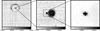 |
Fig. 4 Left: 2k × 2k image of a single NISP detector showing the first-order dispersed image of a monochromatic PSF at 1800 nm taken with NISP RGS000. The corresponding zeroth order is not visible in this image because it falls into detector gaps about 800 pixels above the first-order PSF. Centre: zoom-in showing the surrounding area of the PSF in a region of 40 × 40 pixels. Right: zoom in on a region of 10 × 10 pixels centred on the PSF. Here, the colour scale has been adapted to not have the central core of the PSF saturated as in the left and central image. For a detailed description of image features, see the main text. |
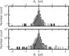 |
Fig. 5 Differences in the measured position of the PSF centroid for the various models used. Top: difference in position in the cross-dispersion direction (δ⊥). Bottom: difference in position in the dispersion direction (δ∥). In both panels, the number count axis is logarithmic. The black histogram compares the elliptical Moffat profile to the dual-Gaussian profile. The grey histogram compares the asymmetric-Gaussian profile to the dual-Gaussian profile. The light grey histogram compares the asymmetric-Gaussian profile with the elliptical Moffat profile. |
4.2 Addressing RGS270 non-conformity
One consequence of the Euclid telescope (Refregier et al. 2010; Laureijs et al. 2011; Euclid Collaboration: Mellier et al. 2025) having an off-axis three-mirror Korsch design (Korsch 1977) is that in order to obtain high-quality images at all positions the NISP focal plane has to be tilted by an angle of 4.◦8267 with respect to the optical axis (Euclid Collaboration: Jahnke et al. 2025), as illustrated in Fig. 8. The grisms RGS000 and RGS180 are dispersing light in the direction parallel to the zNISP axis, i.e. perpendicular to the focal plane tilt. For this reason the focal length for exactly (and only) these two specific dispersions directly is identical for all wavelengths of a given object, as in an on-axis telescope. On the other hand for grism RGS270, with a dispersion direction perpendicular to RGS000 and RGS180, the dispersion is running in a direction perpendicular to the zNISP axis, i.e. in the direction of the focal plane tilt. The curvature of the grating grooves in the RGS270 grism design was introduced specifically to correct for the tilt of the NISP focal plane, creating in-focus images on the focal plane at any wavelength.
However, during our ground test campaign at instrument level we observed that images from grism RGS270 were partially defocused. This can be seen in Fig. 9, which compares Fabry–Pérot spectrograms acquired with RGS000 and RGS270 during NISP ground test campaign. Focusing on the middle image presenting the RGS270 2D spectrogram, one can see that the bluest part of the spectrum (left-hand side) has a narrow and well focused PSF. In contrast to this, with increasing wavelength towards the right, the PSF gets successively wider and at the reddest end even shows a ring-like appearance. There is clearly an increasing de-focus with increasing wavelength.
After investigations, we concluded that the RGS270 grism was built using an improper interpretation of its optical design: the definition of the RGS270 optical reference frame was not properly propagated to the NISP mechanical reference frame – which are oriented inversely to each other. The main consequence of this error resulted in all models built for RGS270 to disperse light in the opposite direction to the design definition. As a result the focus compensation by the curved grating groove was going in the wrong direction.
A ‘Tiger Team’ composed of Euclid Consortium members investigated potential hardware solutions, including various possibilities to replace the RGS270 grisms that were built, as well as options to modify Euclid’s surveys. After an assessment of both the risks for the mission induced by dismantling the NISP instrument and the time required to build a new RGS270 grism, a survey solution was proposed by the consortium and approved by the ESA. This was based on a detailed analysis of a modification of survey and observation parameters, which we discuss in the following.
To obtain the additional spectral orientation angles needed for decontamination of overlapping spectra, the survey >solution involved to modify the survey strategy using NISP settings that rotate the NI-GWA by ±4◦ away from its nominal positioning of the grisms with respect to the centre of the beam, when observing with either RGS000 or RGS180. This in turn creates spectra tilted by ±4◦ versus the nominal orientation of spectra from RGS000 and RGS180. After an in-depth simulation of different survey strategies we ended up with an optimal spectroscopic observation sequence. Each field is observed four times, with grisms used in the following order: RGS000 → RGS180+4◦ → RGS000–4◦ → RGS180.
The advantage of this observation sequence, executed in the ‘K pattern’ of telescope dithering offsets for each sky position (Euclid Collaboration: Scaramella et al. 2022; Euclid Collaboration: Mellier et al. 2025), creates a geometry formed by the stacked spectra that offers even more dispersion angles than the initial observation sequence, for disentangling spectra during the offline data processing on the ground. The largest drawback is that by slight rotation angle of the grism wheel, the nominal aperture of the grism – defined by a baffle installed in front of the grating – is shifted away from the nominal beam centre, introducing slight vignetting at the edge of the FoV. This vignetting has been estimated from Zemax simulation to result in 10% flux losses at ±0.◦385 field angle, i.e. distance from the centre of the FoV, which is reduced to 0% flux losses at field angle <0.◦17. A on-sky simulation, involving the official Euclid data reduction pipeline, demonstrated that this vignetting level is largely compensated for by the detector quantum efficiency and an optical throughput, which are both higher than scientifically required, and that the spatial structure can also easily be accounted for in the pipeline. Larger tilts were also investigated but the increasing vignetting level quickly reduces the options for modifying the Euclid survey strategy along this line.
As a conclusion, the RGS270 is kept on board the NISP instrument to maintain the centre of gravity during mission operation, but it will not be used for Euclid’s surveys. While an extensive dataset was acquired for RGS270 during ground testing, in the following the performance of RGS270 is not discussed any further.
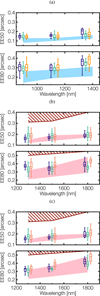 |
Fig. 6 NISP grism image quality as a function of wavelength, compared to the expectation from an ideal model limited by optical diffraction (shaded region) and to NISP scientific requirements (dashed region), for the grisms BGS000 (a), RGS000 (b), and RGS180 (c). For each grism, the upper panel shows the EE50 estimated with the asymmetric-Gaussian (dark blue), dual-Gaussian (green), and Moffat profile (yellow). The bottom panel shows the corresponding EE80. An artificial wavelength shift was applied to increase readability. |
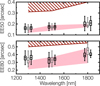 |
Fig. 7 No image quality change between nominal and ±4◦ offsets. Compared are EE50 (top panel) and EE80 (bottom panel) for nominal and offset positions, combining data from RGS000 and RGS180. The central grey boxes at 1300 nm, 1500 nm, and 1800 nm correspond to the encircled energy measured with the grism wheel in nominal position. The boxes to its left and right correspond to measurements done with −4◦ and +4◦ offsets, respectively. An artificial wavelength shift was applied to increase readability. For clarity, the plot is restricted to the encircled energy estimate using the asymmetric-Gaussian profile. |
 |
Fig. 8 Ray tracing of the NISP Optical Assembly for three sources located at the centre and at two opposing edges of the focal plane. Light rays are shown, for each source, at wavelengths of 1250 nm (red), 1550 nm (green), and 1850 nm (blue), dispersed by grism RGS270. The dichroic element is located in the pupil plane of the telescope outside of NISP and is not part of the instrument. |
 |
Fig. 9 Top: image of the Fabry–Pérot etalon spectrum acquired with the NISP grism RGS000 during the instrument test campaign. Middle: image of the Fabry–Pérot etalon spectrum acquired with the NISP grism RGS270 during the instrument test campaign. Bottom: spot size of the Fabry– Pérot emission lines displayed as radial profiles at 1300 nm (A), 1540 nm (B), and 1840 nm (C). Measurement points are marked by open circle for RGS000 and dots for RGS270. The dashed lines are a radial-profile fit with a double Gaussian to emphasise the shape of the PSF. This functional form allows one of the two Gaussian to have the negative amplitude needed to reproduce the ring-shape of the RGS270’s PSF at large wavelengths. |
5 NISP spectroscopic dispersion
An important part of the NISP ground test campaign was to establish a preliminary assessment of the grism’s dispersion law as mounted inside the instrument, in preparation for the instrument calibration in-flight and NISP’s in-flight operations. This section details the procedure used to calibrate the NISP spectral dispersion on the ground, explaining how the calibration datasets were acquired and analysed, before we discuss the validity and precision of this calibration.
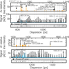 |
Fig. 10 Calibration spectra for the NISP BGS000 (upper panel) and RGS000 grisms (lower panel). For each grism the 2D image of the argon spectral lamp spectrum is shown at the bottom, the argon 1D spectrum (cyan) compared to the Fabry–Pérot etalon spectrum (black) in the centre, and the reference argon spectrum in vacuum from Kramida et al. (2022) at the top. |
5.1 On-ground spectral dispersion calibration
To estimate spectral dispersion functions of the NISP grisms, the Fabry–Pérot etalon spectrum was projected with the telescope simulator to 144 individual points on the NISP FoV. For every pointing a short exposure of ≃13 s was taken before the telescope simulator moved to the next field point. Additionally, at all positions corresponding to the centre of a NISP detector, we also used the argon spectral lamp to obtain spectra as reference and control.
To avoid any bias induced by a small but still different alignment of the grism wheel after multiple repositioning, all measurements at these 144 points were made without turning the grism wheel. Only once a 144-pointing scan with a given grism was completed, the grism wheel was moved to position the next grism. This test sequence was used for all four grisms – meaning the grisms BGS000, RGS270, RGS000, and RGS180 each at nominal positioning as well with the grisms RGS000 and RGS180 with a ±4◦ rotation offset. Also, from the point of view of the calibration, we chose to consider the rotated grism positions RGS000±4◦ and RGS180±4◦ to be independent grisms of their own and not to consider them to be identical to RGS000 or RGS180.
Before going into the details of the calibration, Fig. 10 presents examples of the first-order spectrogram for the blue and red grisms acquired during the NISP ground tests. The middle panels each show and compare spectrograms of the Fabry–Pérot etalon with those of the argon spectral lamp. The top panels show reference argon spectra in vacuum in these wavelength ranges, taken from the National Institute of Standards and Technology (NIST) database (Kramida et al. 2022). By comparing the reference argon spectra with those observed with NISP (middle and bottom panels) one can identify the strongest argon emission lines present in both the BGE and RGE bandpasses. The middle panels also identify the Fabry–Pérot transmission peaks. For clarity, we limit the labelling to two peaks but based on the Fabry–Pérot calibration data all other transmission peaks were clearly identified2. The middle and bottom panels do not cover the spectrogram of the zeroth order, which is located about 500 pixel away off the left-hand side.
Upon close inspection of the bottom panels, we can see that both show a slight periodic excess. This is a charge persistence signal from the previous Fabry–Pérot etalon exposure. However, persistence did not affect the exposure of the Fabry–Pérot etalon itself, since the pointing position was changed between subsequent exposures and the Fabry–Pérot light source was brighter than the spectral lamp.
One central calibration for the NISP grisms is to describe the relation to convert wavelength for a source at any position into a position onto the focal plane. This is first established independently for each of the 144 spectrograms by modelling the 2D spectral trace with the following parametric function:
 (2)
(2)
Here (y, z) are spatial coordinates of a spectral feature on the focal plane, with y and z axis defined to be parallel to RGS000’s cross-dispersion and dispersion direction, respectively. (y0, z0) are spatial reference coordinates, Ti/j(λ′), are Chebyshev polynomials of the first kind defined in the [λmin, λmax] wavelength range, and Cκ the Chebyshev coefficients, with κ being either y or z. The (y, z) coordinates of the Fabry–Pérot transmission peaks were measured by fitting the observed peaks with the PSF profile described in Sect. 4, providing position with an accuracy of ≃1/10th of a pixel.
This work uses as a reference the centroid position of the spectral zeroth order, which is defined to be the position of the in-band zeroth order’s wavelength with minimal transmission. This reference position is estimated from a template fit of the 2D image of the zeroth-order spectrogram with a Fabry–Pérot template.
The transmission of the optical ground equipment has some residual knowledge uncertainties. To limit the impact of this, the Fabry–Pérot template is constructed by taking the averaged profile of its first-order spectrogram measured with the corresponding grism, corrected by the first-order transmission efficiency. In this way the template is considered to be representative of the photon flux at the entrance pupil of the NISP instrument. To account for the zeroth order, the template is then multiplied by the zeroth-order transmission efficiency (see Fig. 3) and convolved with a PSF profile before being adjusted to the 2D images of the zeroth order. Parameters of the fit are (i) the centroid position of the template, defined to be the central wavelength of the grism band-pass, where the zeroth-order transmission efficiency is at its minimum, (ii) a stretch factor converting wavelength to pixel, (iii) the dispersion direction angle, and (iv) parameters of the PSF profile defined in Sect. 1, which account for the contribution of the fibre core.
An example of such a template fit is shown in Fig. 11, which presents the measured image of the Fabry–Pérot zeroth-order spectrogram in (A) with the model in (B) and the residual in (C) and (D). Due to the prisms onto the NISP’s grisms, the zeroth order are slightly dispersed, extending over several tens of pixels. Additionally, the grating’s blaze function is optimised to maximise transmission in the first order – around 1500 nm for the red grisms and 1100 nm for the blue grism – while minimising transmission at the same wavelengths for the zeroth order. As a result, instead of appearing as a point-like feature, as would be expected for a purely dispersive grating, NISP’s zeroth order takes the form of an elongated, double-peaked structure. We tested the different PSF profiles we listed in Sect. 4 and concluded that they all provide similar results without any of them outperforming the others. As for modelling the monochromatic PSF, the usage of either of the profiles described in Sect. 4 led to similar centroiding of the zeroth order with negligible impact on the derived calibration parameters. The zeroth-order position errors at 1σ were determined using χ2-profiling and subsequently propagated to the centroid position of the Fabry–Pérot transmission peaks during the calibration of individual first-order spectrograms. Analysing the distribution of measured uncertainties in the zeroth-order positions, we obtain mean uncertainties of 0.051 ± 0.006, pixels with a standard deviation of 0.15 pixels in the cross-dispersion direction and 0.12 ± 0.02, pixels with a standard deviation of 0.4 pixels in the dispersion direction. This highlights that positioning is more precise in the cross-dispersion direction, as the profile of the zeroth order is significantly thinner in this direction, leading to better constraint.
Coefficients of the Chebyshev polynomial as described in Eq. (2) are evaluated from a recursive χ2-fit. In the recursion, outliers were rejected at every iteration, each identified as spectral features located >5σ away from the fitted spectral trace. Recursion stopped when no further outlier were identified. This allowed us to automatically reject some of the Fabry–Pérot transmission peaks that were insufficiently characterised by our PSF modelling due to nearby hot or bad pixels. Chebyshev polynomials were expanded up to the third order in the cross-dispersion direction and up to the fourth order in the dispersion direction. For the blue grism calibration the expansion was limited to the third order in both directions. The level of the expansion order was chosen in order for the averaged reduced χ2 to be the closest to 1. With the above expansion order, the averaged reduced χ2 is of the order of 0.92±0.03. However, we noticed that the χ2 distribution is skewed towards lower values. This is due to the limited accuracy of the template fit on a few of the zeroth-order images that propagated to the first-order spectra and leads to large uncertainties in the relative position errors of some peaks’ positions, (y − y0).
Up to this point, the Fabry–Pérot spectrograms were modelled independently of each other, leading to calibration coefficients  that smoothly vary across the FoV depending on the location of the zeroth order. To complete the calibration, the spatial dependence of each of the
  coefficients is then fitted by a bi-dimensional Chebyshev polynomial defined as
 (3)
(3)
with aij the calibration parameters to be evaluated and Ti/j(κ′) the Chebyshev polynomials of the first kind, with κ′ being either y′ or z′ defined in the ![Mathematical equation: $\left[ {\kappa _{\min }^\prime ,\kappa _{\max }^\prime } \right]$](/articles/aa/full_html/2026/03/aa55859-25/aa55859-25-eq12.png) range as
range as
 (4)
(4)
Here ![Mathematical equation: $\left[ {\kappa _{\min }^\prime ,\kappa _{\max }^\prime } \right]$](/articles/aa/full_html/2026/03/aa55859-25/aa55859-25-eq14.png) are the limits of the focal plane array, set to [−85, +85] mm for both the y and z axes. Again, the evaluation of the aij parameters is carried out by a χ2 fit. The tables that summarise the calibration coefficients for each of the grisms are presented in Appendix A. The advantage of Eq. (2) is that, through the set of coefficients
are the limits of the focal plane array, set to [−85, +85] mm for both the y and z axes. Again, the evaluation of the aij parameters is carried out by a χ2 fit. The tables that summarise the calibration coefficients for each of the grisms are presented in Appendix A. The advantage of Eq. (2) is that, through the set of coefficients  , it simultaneously describes the spectral dispersion and the curvature of the spectra, including non-linear effects induced by optical field distortion. Furthermore, by modelling each
  coefficient over the entire FoV using Eq. (3), one directly obtains a 2D mapping of both dispersion and curvature through the higher-order coefficients i or j greater than or equal to 2.
Theoretically, in a perfect optical system with constant grating groove, one expects the spectrograms to rotate around their un-deflected wavelength when the grating is rotated around its centre. However, with the complexity of the NISP instrument itself, the mechanical uncertainties on the wheel position after its rotation, and on the pointing of the telescope simulators, it was not possible to precisely measure and confirm the position of the rotation centre for each of the spectrograms. The choice was made to minimise the bias induced by the uncertainty on the location of each spectrum’s centre of rotation by considering each grism’s orientation as an independent grism to be calibrated. We tested the hypothesis that the rotation centre of the spectrograms was either their un-deflected wavelength or the zeroth order3. However, the calibration error derived from such a nominal position was found to be outside of our scientific requirement once it was applied to the rotated grisms, despite being calculated at the sub-pixel level.
Once we obtained the calibration parameters, we computed a predicted position of the Fabry–Pérot emission line using Eqs. (2) and (3) and compared the reconstructed and measured positions. This comparison is shown in Fig. 12. For clarity, we only show the results of the comparison for the blue grism BGS000 (in blue) and for the combined distribution of RGS000 and RGS000±4 (in yellow) as well as for the combined distribution of RGS180 and RGS180±4 (in purple). The calibration error we derived from this comparison is found to be lower than 7 × 10⁻⁴ mm (i.e. < 0.04 pixel) in the cross-dispersion direction and lower than 1 × 10⁻³ mm (i.e. <0.06 pixel) in the dispersion direction for each grism.
Additionally, we noticed that every spectrum for which the zeroth and first orders were located on two different detectors shows a local offset in the estimated values of both the  and
and  coefficients, while the higher order coefficients of the parametrisation remained compatible with the coefficients estimated for any spectrogram fully falling onto a single detector. This offset behaves as if those spectra have a longer separation between the position of their zeroth and first orders, breaking the otherwise rather smooth variation of the
  and
and  coefficients across the FoV. Instead, we concluded that this offset has its origin in a bias induced by a limited precision of the detector metrology: this provides physical positions of the NISP detectors within the focal plane and was used to convert positions measured in pixels on a given detector to positions in the NISP focal plane reference frame. However, the detector metrology was only determined at room temperature by measuring the position of reference marks engraved on the mechanical structure of each detector, using an optical camera mounted on a metrology bench. This method only provided a precision of the order of one pixel (i.e. ≃18 µm). The NISP focal plane metrology at operational temperature was therefore computed relying on the thermal model of the NISP instrument to predict, with limited precision, how thermal stress would modify the focal plane.
We tried to re-calibrate the detector metrology at cold using the spectroscopic data themselves by aligning first-order spectra dispersed over multiple detectors. However, due to the small number of sources available (i.e. one single spectrum per NISP exposure in the entire NISP focal plane), a re-computation with sufficient precision for the spectroscopic calibration was not possible. We therefore left our cold reference-metrology as is and checked that the calibration parameters remain within 3σ when computing calibration parameters with or without the spectra showing an offset in the  and
and  coefficients.
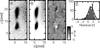 |
Fig. 11 Example of the outcome of a template fit of the zeroth-order spectrogram. Panel A: image of the Fabry–Pérot zeroth-order spectrogram as acquired by the RGS000. Panel B: modelled image resulting from the template fit. Panel C: residual of the template fit. Panel D: residual distribution. |
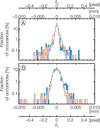 |
Fig. 12 Normalised histograms of the distance between measured Fabry–Pérot emission lines and their positions predicted from calibration parameters in the cross-dispersion direction, δ⊥ (A), and in the dispersion direction, δ∥ (B), for BGS000 (blue), RGS000 and RGS000±4 combined (yellow), and RGS180 and RGS180±4 combined (purple). |
5.2 Validation of the spectroscopic dispersion law
During the NISP ground test campaign, we acquired 16 spectrograms of the argon spectral lamp with each of the BGS000, RGS000, and RGS180. An argon spectrogram was observed every time the telescope simulator pointed to the centre of one of the 16 NISP detectors. This was achieved by replacing the Fabry–Pérot’s fibre feeds within our optical ground equipment with feeds connected to the argon spectral lamp. No other modifications were made to the instrument configuration or telescope simulator pointing. These argon spectrograms were used to validate the spectroscopic dispersion law that we derived from the Fabry–Pérot etalon calibration.
Similar to what was done for the Fabry–Pérot’s spectrogram, we extracted argon emission line positions based on model fitting of the 2D emission line profile. However, the detection process was significantly impacted by a substantial level of detector persistence charge signal from the previous Fabry–Pérot’s exposure acquired at the same pointing as for the spectral lamp acquisition. A visual inspection of the initially identified line was conducted, to reject persistence signal peaks that are miss-identified as argon emission lines by the automated peak-search algorithm, as well as ambiguous line detection. In the cases where it was challenging to differentiate between actual emission lines and persistence signal, the line was masked from the analysis.
Additionally, we extracted the zeroth-order position from a template fit, replacing the Fabry–Pérot template with the argon spectral energy distribution (SED) template whenever the zeroth order was visible on the 2D spectrogram. This was primarily possible for acquisitions with the BGS000 grism. Contrary to this, the signal was below the detectable signal-to-noise ratio for the red grisms. Since we did not move the telescope simulator when changing the light source, we assumed for those cases that the zeroth-order position of the argon spectrogram was the same as that of the Fabry–Pérot spectrogram from the previous exposure.
When inspecting argon spectrograms captured with the BGS000, we found that four of them had very weak signal for the zeroth order resulting in the template fit failing to converge, positioning the zeroth order at about seven pixels away from visually determined position. These spectra were also excluded from our analyses.
Using calibration parameters that were derived from the Fabry–Pérot spectrogram analysis (see Sect. 5.1), we estimated the position of the argon emission lines relative to the zeroth-order position and compared the predicted positions with the measured position. The bias resulting from this comparison is reported in Table 1, defined as the average of the distribution as shown in Fig. 13. It is induced by the persistence present in the images that tend to bias either the centroiding of the argon lines themselves or the estimate of the zeroth-order position. As was described above, for the BGS000 an argon SED template was used to evaluate the zeroth-order position, while for both red grisms this was taken from the previous exposure, assuming the telescope did not move between exposures. As a consequence, the weakness of the zeroth order and the persistence signal present in the BGS000 spectrogram leads to a larger bias than what is observed for the corresponding distribution of the red grisms. Nonetheless, despite this bias, we found that the predicted position of the argon lines fall within a distance of ≃0.5 pixels of the measured lines, which validates our calibration parametrisation.
Average distance, standard deviation, and mean bias error between measured and predicted argon line positions across NISP’s FoV.
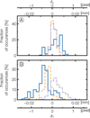 |
Fig. 13 Histograms of the distances between measured and predicted argon line positions across the NISP FoV in the cross-dispersion direction, δ⊥ (A), and in the dispersion direction, δ∥ (B) – for the argon spectrograms captured with BGS000 (blue line), RGS000 (dashed yellow line), and RGS180 (dot-dashed purple line). |
6 NISP spectroscopic performance
While calibration parameters have been computed on the basis of Chebyshev polynomials, it is more convenient to convert the obtained spectroscopic dispersion laws into regular polynomials to assess properties and performance of the grism’s dispersion. In that case, the dispersion laws take the following form:
 (5)
where
(5)
where  , with κ being either y or z, are the regular polynomial coefficients in cross-dispersion (κ = y) and dispersion direction (κ = z). When converted to regular polynomials, the coefficients of zero degree
  are related to the Cartesian distance that separate the first order of the spectra to the reference used in this work, i.e. the position of the zeroth order. The first degree coefficients
  are related to the dispersion dλ/dκ of the spectra while coefficients of higher degree define the curvature of the spectra, which is linked to the non-linearity of the dispersion law and optical distortions of the system.
For clarity and simplicity, the forthcoming discussion is confined to the description of the dispersion law averaged over the NISP FoV. Table A.1 reports the dispersion coefficients in both the Chebyshev and regular basis and reveals that when the grisms are centred onto their nominal position, the cross-dispersion coefficient  is about two orders of magnitude lower than the dispersion coefficient
  . This aligns with the intended design of the grisms, which primarily focuses on dispersing light in a single direction. Optical and mechanical distortions as well as the manufacturing limitations contribute to the distortion of the spectral track in both directions. However, even with those limitations, the higher-order coefficients (
 with i > 1) are small enough for the dispersion to be nearly a linear dispersion law mostly directed towards the z axis.
In contrast, when the grisms are tilted by ±4◦, the cross-dispersion coefficient  increases to be one order of magnitude lower than the dispersion coefficient
  . This discrepancy with the nominal position arises due to the dispersion occurring in both directions when the dispersion grating is rotated by ±4◦.
Under the formalism used in this work, the dispersion of NISP’s grisms predominantly takes place in the z direction. As a consequence, our focus now shifts to the discussion of the regular Pz polynomials.
In the context of slitless spectroscopy, spectral resolution is defined by a combination of both the intrinsic instrument PSF and the characteristics of the targeted object’s size, shape, and surface brightness distribution. Referring to the definition provided in Euclid’s scientific requirement, we define NISP’s resolving power ℛ as
 (6)
(6)
Here, ∆λ corresponds to the per-pixel spectral dispersion along the dispersion direction4 and is expressed in µm/px. The  corresponds to the FWHM of the target source with an axisymmetric Gaussian profile of effectives variance
  . This effective FWHM results from the convolution between the luminosity profile of the source and the PSF and can be expressed as
 (7)
(7)
The FWHMPSF(λ) is the FWHM of the PSF, in pixels, at a given wavelength λ, and FWHMsrc corresponds to the FWHM, in pixels, of the target and depends on the source’s surface brightness distribution.
When considering grisms RGS000 and RGS180 in their nominal position, the regular polynomial Pz(λ) given in Eq. (5) describes the parametrisation for the grism’s dispersion law in the dispersion direction. Its first-order coefficient (wz1) can be related to the grism’s dispersion (dz/dλ). To obtain an estimate of the per-pixel dispersion ∆λ = dλ/dz one needs to first invert this polynomial. Given our parametrisation, Pz(λ) is continuously differentiable and non-null in the bandpass of the grisms; hence, Pz(λ) is invertible in the neighbourhood of λ, with its inverse also being differentiable at b = Pz(λ) such that
 (8)
(8)
The constant term in the derivative of the inverse function  gives an estimate of the dispersion ∆λ at a wavelength λ within in the grism’s bandpass.
Figure 14 presents the variation across the FoV of the dispersion coefficients at the mid-bandpass wavelength, for all combinations of grism’s rotation that were tested. The dispersion smoothly varies across the NISP FoV following a radial gradient with its maximum, or minimum, on the left-hand side of the focal plane at about mosaic coordinates (−80, 0) mm. Notice the difference between the two red grisms: RGS000 has an average dispersion of the order of +1.37 nm px−1 while RGS180’s average dispersion is of the order of −1.37 nm px−1. The negative sign of the RGS180 dispersion originates from its design, which imposes a dispersion of the light in the opposite direction from RGS000. But on overall, RGS000 and RGS180 have a very similar absolute dispersion in terms of value and profile over the focal plane array, leading to a similar performance for both grisms. Note that, to highlight these similarities and due to the negative dispersion value of RGS180, colour scale for RGS180 is reversed relative to that of RGS000. In contrast, BGS000 has a lower dispersion with an average value of the order of 1.24 nm px−1. All these values are compatible with the design-specifications for each grism.
Combining this estimate of the dispersion with the measured PSF size, NISP’s resolving power can be derived using Eqs. (6) and (7). The result is summarised in Fig. 15, which shows NISP’s averaged resolving power for a source of 0.″5 FWHM. The averaged resolving power from the blue grism increases from about ℛ ≃ 440 at 900 nm to ≃690 at 1300 nm, while both red grisms see their resolving power increase from ℛ ≃ 550 at 1300 nm to ≃740 at 1800 nm. These values have to be compared to the NISP scientific requirements of a resolving power ℛ ≥ 260 for the blue grism and ℛ ≥ 380 for the red grisms and for a typical source size of 0.″5. The combination of the high optical quality of the grisms and the NISP camera and collimator lenses ensures that NISP fulfils its requirements in terms of spectral dispersion and resolving power.
In addition to the measurements described in this work, ground tests were conducted to verify compliance with stray light requirements from in-field and out-of-field sources. These confirmed that parasitic signals are below scientific performance thresholds. No further characterisation was done, as the objective was limited to performance verification and time dedicated to the test campaign was constrained.
Again, shorter tests were conducted at the PLM level with the addition of the Euclid mirrors and dichroic element to the light path. This allowed us to verify that the addition of the folding mirrors as well as the transmission of the NIR light beam through the dichroic did not significantly modify NISP’s spectral dispersion, resolving power as well as optical performances.
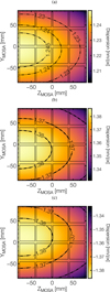 |
Fig. 14 NISP’s grism dispersion across the NISP focal plane reference frame identified as ℛMOSA, with MOSA standing for the pixel mosaic: blue grism BGS000 dispersion at 1 µm (a), red grism RGS000 dispersion at 1.5 µm (b), and red grism RGS180 dispersion at 1.5 µm (c). In each panel, the squares represent the physical positions of the NISP detectors. In this representation we see the focal plane as an incoming photon will see it. |
7 Conclusions and available data products
The NISP instrument integration was completed in 2019. Before its delivery to ESA for its integration into the PLM of the Euclid spacecraft, the NISP instrument underwent a series of tests in a vacuum and cold environment to validate its operation mode as well as to validate its performance in view of the forthcoming flight operation. During the test campaigns that took place in the beginning of 2020, the optical performance of NISP was verified.
One of the measurement campaigns conducted under vacuum at cold temperatures was dedicated to the verification of the image quality provided by NISP’s grisms as well as to the verification and validation of their dispersion. These are key properties in the accurate determination of the cosmological redshifts needed to derive cosmological parameters in galaxy clustering analyses.
While a non-conformity was revealed for the grism RGS270, which resulted in the modification of the Euclid survey strategy, the analysis of the ground dataset presented in this work shows that NISP’s grisms BGS000, RGS000, and RGS180 have an extremely high image quality with a PSF encircled energy size well below the scientific requirements and very close to that of an ideal, solely diffraction-limited instrument.
Secondly, these tests allowed us to verify that the spectral dispersion of NISP lies above requirements and showed that NISP’s resolving power (ℛ) is greater than 480 from 1000 nm to 1800 nm. The RGS000, RGS180, RGS270, and BGS000 throughput for the zeroth and first spectral orders at the centre of the NISP focal plane array are available at an ESA server5. Available throughput numbers include contributions from the grisms, the telescope, and NISP Optical Assembly (NI-OA), as well as the mean detector quantum efficiency. For convenience, the tables are available in both ASCII and FITS format.
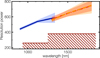 |
Fig. 15 NISP’s averaged resolving power for the BGS000 (line), RGS000 (dashed), and RGS180 (dot-dashed) grisms as a function of wavelength, assuming a source size of 0.″5 FWHM. The shaded areas illustrate the variation in the resolving power due to the variation in the PSF and the variation in the dispersion, ∆λ, across the FoV. The hatched region shows the ‘forbidden’ region below the scientific requirements. |
Acknowledgements
The Euclid Consortium acknowledges the European Space Agency and a number of agencies and institutes that have supported the development of Euclid, in particular the Agenzia Spaziale Italiana, the Austrian Forschungsförderungsgesellschaft funded through BMK, the Belgian Science Policy, the Canadian Euclid Consortium, the Deutsches Zentrum für Luft- und Raumfahrt, the DTU Space and the Niels Bohr Institute in Denmark, the French Centre National d’Etudes Spatiales, the Fundação para a Ciência e a Tecnologia, the Hungarian Academy of Sciences, the Ministerio de Ciencia, Innovación y Universidades, the National Aeronautics and Space Administration, the National Astronomical Observatory of Japan, the Netherlandse Onderzoekschool Voor Astronomie, the Norwegian Space Agency, the Research Council of Finland, the Romanian Space Agency, the State Secretariat for Education, Research, and Innovation (SERI) at the Swiss Space Office (SSO), and the United Kingdom Space Agency. A complete and detailed list is available on the Euclid web site (www.euclid-ec.org).
References
- Bodendorf, C., Geis, N., Grupp, F., et al. 2019, Astronomical optics: Design, manufacture, and test of space and ground systems II, eds. T. B. Hull, D. W. Kim, & P. Hallibert, 11116, 111160Y [Google Scholar]
- Bonnefoi, A., Bon, W., Niclas, M., et al. 2016, Space telescopes and instrumentation 2016: Optical, infrared, and millimeter wave, eds. H. A. MacEwen, G. G. Fazio, M. Lystrup, et al., 9904, 99042V [Google Scholar]
- Bougoin, M., Lavenac, J., Pamplona, T., et al. 2017, in International Conference on Space Optics – ICSO 2016, 10562 (SPIE), 1329 [Google Scholar]
- Boyd, J. P. 2006, J. Sci. Comput., 29, 1 [Google Scholar]
- Costille, A., Caillat, A., Grange, R., Pascal, S., & Rossin, C. 2014, in Advances in Optical and Mechanical Technologies for Telescopes and Instrumentation, 9151, eds. R. Navarro, C. R. Cunningham, & A. A. Barto, International Society for Optics and Photonics (SPIE), 91515E [Google Scholar]
- Costille, A., Beaumont, F., Prieto, E., Carle, M., & Fabron, C. 2016a, in Advances in Optical and Mechanical Technologies for Telescopes and Instrumentation II, 9912 (SPIE), 1390 [Google Scholar]
- Costille, A., Carle, M., Fabron, C., et al. 2016b, in Proceedings of SPIE – The International Society for Optical Engineering, 9904 [Google Scholar]
- Costille, A., Carle, A., Beaumont, F., et al. 2017, in International Conference on Space Optics – ICSO 2016, 10562 (SPIE), 937 [Google Scholar]
- Costille, A., Beaumont, F., Prieto, E., et al. 2018, in Advances in Optical and Mechanical Technologies for Telescopes and Instrumentation III, 10706 (SPIE), 498 [Google Scholar]
- Costille, A., Caillat, A., Rossin, C., et al. 2019, International Conference on Space Optics — ICSO 2018, 11180, 1118013 [Google Scholar]
- Cropper, M., Pottinger, S., Niemi, S., et al. 2016, in Space Telescopes and Instrumentation 2016: Optical, Infrared, and Millimeter Wave [Google Scholar]
- Euclid Collaboration (Scaramella, R., et al.) 2022, A&A, 662, A112 [NASA ADS] [CrossRef] [EDP Sciences] [Google Scholar]
- Euclid Collaboration (Schirmer, M., et al.) 2022, A&A, 662, A92 [NASA ADS] [CrossRef] [EDP Sciences] [Google Scholar]
- Euclid Collaboration (Cropper, M., et al.) 2025, A&A, 697, A2 [Google Scholar]
- Euclid Collaboration (Jahnke, K., et al.) 2025, A&A, 697, A3 [Google Scholar]
- Euclid Collaboration (Mellier, Y., et al.) 2025, A&A, 697, A1 [Google Scholar]
- Grupp, F., Prieto, E., Geis, N., et al. 2012, in Space Telescopes and Instrumentation 2012: Optical, Infrared, and Millimeter Wave, 8442 (SPIE), 358 [Google Scholar]
- Jiang, J., Lei, L., & Guangjun, Z. 2016, Opt. Eng., 55, 063101 [Google Scholar]
- Korsch, D. 1977, Appl. Opt., 16, 2074 [NASA ADS] [CrossRef] [Google Scholar]
- Kramida, A., Ralchenko, Y., Reader, J., & Team, N. A. 2022, National Institute of Standards and Technology, Gaithersburg, MD, version 5.10 [Online] [Google Scholar]
- Laureijs, R., Amiaux, J., Arduini, S., et al. 2011, arXiv e-prints [arXiv:1110.3193] [Google Scholar]
- Le Graët, J., Secroun, A., Barbier, R., et al. 2022, in Society of Photo-Optical Instrumentation Engineers (SPIE) Conference Series, 12191, X-Ray, Optical, and Infrared Detectors for Astronomy X, eds. A. D. Holland, & J. Beletic, 121911M [Google Scholar]
- Lucy, L. B. 1974, AJ, 79, 745 [Google Scholar]
- Maciaszek, T., Ealet, A., Jahnke, K., et al. 2016, in Space Telescopes and Instrumentation 2016: Optical, Infrared, and Millimeter Wave, 9904, eds. H. A. MacEwen, G. G. Fazio, M. Lystrup, et al., International Society for Optics and Photonics (SPIE), 99040T [Google Scholar]
- Maciaszek, T., Ealet, A., Gillard, W., et al. 2022, in Space Telescopes and Instrumentation 2022: Optical, Infrared, and Millimeter Wave, 12180, eds. L. E. Coyle, S. Matsuura, & M. D. Perrin, (SPIE), 121801K [Google Scholar]
- Moffat, A. F. J. 1969, A&A, 3, 455 [NASA ADS] [Google Scholar]
- Moore, K. E., Nicholson, M. G., & Warwick, J. R. 2004, in Optical Design and Engineering, 5249, ed. L. Mazuray, P. J. Rogers, & R. Wartmann, (SPIE), 400 [Google Scholar]
- Refregier, A., Amara, A., Kitching, T. D., et al. 2010, Euclid Imaging Consortium Science Book, [arXiv:1001.0061] [Google Scholar]
- Richardson, W. H. 1972, J. Opt. Soc. Am., JOSA, 62, 55 [Google Scholar]
- Riva, M., Carty, J., Barriere, J., et al. 2011, in 14th European Space Mechanisms and Tribology Symposium – SPIE Vol. 8442, 14 [Google Scholar]
- Serre, D., Villeneuve, E., Carfantan, H., et al. 2010, in Adaptive Optics Systems II, 7736 (SPIE), 1498 [Google Scholar]
For reference see the calibrated Fabry–Pérot SED in Fig. 2.
This, strictly speaking, is not physically possible given the grism design, but this was nevertheless also tested, since at first approximation the zeroth order could be a proxy for the rotation centre.
Along the z-axis for RGS000 and RGS180 in nominal position and in a mixture of y and z axis when those grisms are at ±4◦ inclination.
Appendix A Ground calibration coefficients
Table A.1 presents the averaged calibration coefficients used to model the spectral dispersion of the NISP grism. The table provides the Chebyshev polynomial coefficients directly derived from a fit of Eq. (3) to the ground dataset for all grisms but RGS270 and averaged over the NISP focal plane surface. For convenience, the table provides as well the equivalent averaged coefficients for regular polynomials. Those were obtained through the analytical transformation from the Chebyshev basis into the regular polynomial basis. Tables A.2 to A.8 give the aij calibration coefficients for Eq. (3), used to model spatial dependence of the  coefficient needed in Eq. (2).
Averaged calibration coefficients given in the Chebyshev basis,  , and in their regular polynomial basis,
  .
.


All Tables
Average distance, standard deviation, and mean bias error between measured and predicted argon line positions across NISP’s FoV.
Averaged calibration coefficients given in the Chebyshev basis, , and in their regular polynomial basis, .
All Figures
|
Fig. 1 Schematic view of the NISP instrument detailing its subsystems. Right: view of the whole instrument as integrated. Left: detailed view with an open wheel cavity, showing the locations of the two wheels to select spectral elements. Not shown are the ‘warm’ electronics, which are used for commands and data processing; they are located away from the main NISP instrument assembly in Euclid’s service module (Maciaszek et al. 2016). The subsystem names and functions are described in the main text. |
| In the text | |
|
Fig. 2 Cross-section of a NISP grisms. The prism wedge (light blue) has an added curved basis surface onto which the filter coating is deposited (yellow), while the grooves of the dispersion grating (dark blue) are directly engraved onto the flat hypotenuse surface of the prism. The grisms are characterised by their prism angle (A), the groove height (H), and the blaze angle (β). |
| In the text | |
|
Fig. 3 Total transmission of the spectra’s first order (solid line) and ten times total transmission of the spectra’s zeroth order (dashed line) for the BGS000 (blue), RGS000 (light red), RGS180 (orange), and RGS270 (dark red) grism channels. The total transmission accounts for the transmission of the grisms themselves, of CoLA and CaLA, and includes the detector quantum efficiency. For comparison, the Fabry–Pérot etalon spectrum (light grey) is shown as measured in the laboratory with a Lambda 900 spectrometer, in arbitrary data units. The contributions from neither the dichroic nor telescope are accounted for in these measurements as Euclid mirrors as well as its dichroic were not emulated during the instrument tests. |
| In the text | |
|
Fig. 4 Left: 2k × 2k image of a single NISP detector showing the first-order dispersed image of a monochromatic PSF at 1800 nm taken with NISP RGS000. The corresponding zeroth order is not visible in this image because it falls into detector gaps about 800 pixels above the first-order PSF. Centre: zoom-in showing the surrounding area of the PSF in a region of 40 × 40 pixels. Right: zoom in on a region of 10 × 10 pixels centred on the PSF. Here, the colour scale has been adapted to not have the central core of the PSF saturated as in the left and central image. For a detailed description of image features, see the main text. |
| In the text | |
|
Fig. 5 Differences in the measured position of the PSF centroid for the various models used. Top: difference in position in the cross-dispersion direction (δ⊥). Bottom: difference in position in the dispersion direction (δ∥). In both panels, the number count axis is logarithmic. The black histogram compares the elliptical Moffat profile to the dual-Gaussian profile. The grey histogram compares the asymmetric-Gaussian profile to the dual-Gaussian profile. The light grey histogram compares the asymmetric-Gaussian profile with the elliptical Moffat profile. |
| In the text | |
|
Fig. 6 NISP grism image quality as a function of wavelength, compared to the expectation from an ideal model limited by optical diffraction (shaded region) and to NISP scientific requirements (dashed region), for the grisms BGS000 (a), RGS000 (b), and RGS180 (c). For each grism, the upper panel shows the EE50 estimated with the asymmetric-Gaussian (dark blue), dual-Gaussian (green), and Moffat profile (yellow). The bottom panel shows the corresponding EE80. An artificial wavelength shift was applied to increase readability. |
| In the text | |
|
Fig. 7 No image quality change between nominal and ±4◦ offsets. Compared are EE50 (top panel) and EE80 (bottom panel) for nominal and offset positions, combining data from RGS000 and RGS180. The central grey boxes at 1300 nm, 1500 nm, and 1800 nm correspond to the encircled energy measured with the grism wheel in nominal position. The boxes to its left and right correspond to measurements done with −4◦ and +4◦ offsets, respectively. An artificial wavelength shift was applied to increase readability. For clarity, the plot is restricted to the encircled energy estimate using the asymmetric-Gaussian profile. |
| In the text | |
|
Fig. 8 Ray tracing of the NISP Optical Assembly for three sources located at the centre and at two opposing edges of the focal plane. Light rays are shown, for each source, at wavelengths of 1250 nm (red), 1550 nm (green), and 1850 nm (blue), dispersed by grism RGS270. The dichroic element is located in the pupil plane of the telescope outside of NISP and is not part of the instrument. |
| In the text | |
|
Fig. 9 Top: image of the Fabry–Pérot etalon spectrum acquired with the NISP grism RGS000 during the instrument test campaign. Middle: image of the Fabry–Pérot etalon spectrum acquired with the NISP grism RGS270 during the instrument test campaign. Bottom: spot size of the Fabry– Pérot emission lines displayed as radial profiles at 1300 nm (A), 1540 nm (B), and 1840 nm (C). Measurement points are marked by open circle for RGS000 and dots for RGS270. The dashed lines are a radial-profile fit with a double Gaussian to emphasise the shape of the PSF. This functional form allows one of the two Gaussian to have the negative amplitude needed to reproduce the ring-shape of the RGS270’s PSF at large wavelengths. |
| In the text | |
|
Fig. 10 Calibration spectra for the NISP BGS000 (upper panel) and RGS000 grisms (lower panel). For each grism the 2D image of the argon spectral lamp spectrum is shown at the bottom, the argon 1D spectrum (cyan) compared to the Fabry–Pérot etalon spectrum (black) in the centre, and the reference argon spectrum in vacuum from Kramida et al. (2022) at the top. |
| In the text | |
|
Fig. 11 Example of the outcome of a template fit of the zeroth-order spectrogram. Panel A: image of the Fabry–Pérot zeroth-order spectrogram as acquired by the RGS000. Panel B: modelled image resulting from the template fit. Panel C: residual of the template fit. Panel D: residual distribution. |
| In the text | |
|
Fig. 12 Normalised histograms of the distance between measured Fabry–Pérot emission lines and their positions predicted from calibration parameters in the cross-dispersion direction, δ⊥ (A), and in the dispersion direction, δ∥ (B), for BGS000 (blue), RGS000 and RGS000±4 combined (yellow), and RGS180 and RGS180±4 combined (purple). |
| In the text | |
|
Fig. 13 Histograms of the distances between measured and predicted argon line positions across the NISP FoV in the cross-dispersion direction, δ⊥ (A), and in the dispersion direction, δ∥ (B) – for the argon spectrograms captured with BGS000 (blue line), RGS000 (dashed yellow line), and RGS180 (dot-dashed purple line). |
| In the text | |
|
Fig. 14 NISP’s grism dispersion across the NISP focal plane reference frame identified as ℛMOSA, with MOSA standing for the pixel mosaic: blue grism BGS000 dispersion at 1 µm (a), red grism RGS000 dispersion at 1.5 µm (b), and red grism RGS180 dispersion at 1.5 µm (c). In each panel, the squares represent the physical positions of the NISP detectors. In this representation we see the focal plane as an incoming photon will see it. |
| In the text | |
|
Fig. 15 NISP’s averaged resolving power for the BGS000 (line), RGS000 (dashed), and RGS180 (dot-dashed) grisms as a function of wavelength, assuming a source size of 0.″5 FWHM. The shaded areas illustrate the variation in the resolving power due to the variation in the PSF and the variation in the dispersion, ∆λ, across the FoV. The hatched region shows the ‘forbidden’ region below the scientific requirements. |
| In the text | |
Current usage metrics show cumulative count of Article Views (full-text article views including HTML views, PDF and ePub downloads, according to the available data) and Abstracts Views on Vision4Press platform.
Data correspond to usage on the plateform after 2015. The current usage metrics is available 48-96 hours after online publication and is updated daily on week days.
Initial download of the metrics may take a while.