| Issue |
A&A
Volume 707, March 2026
|
|
|---|---|---|
| Article Number | A228 | |
| Number of page(s) | 21 | |
| Section | Cosmology (including clusters of galaxies) | |
| DOI | https://doi.org/10.1051/0004-6361/202556177 | |
| Published online | 17 March 2026 | |
Euclid preparation
LXXVIII. Full-shape modelling of two-point and three-point correlation functions in real space
1
Dipartimento di Fisica e Astronomia, Università di Bologna, Via Gobetti 93/2, 40129 Bologna, Italy
2
INAF-Osservatorio di Astrofisica e Scienza dello Spazio di Bologna, Via Piero Gobetti 93/3, 40129 Bologna, Italy
3
INAF-Osservatorio Astronomico di Brera, Via Brera 28, 20122 Milano, Italy
4
INFN-Sezione di Genova, Via Dodecaneso 33, 16146 Genova, Italy
5
Dipartimento di Fisica, Università di Genova, Via Dodecaneso 33, 16146 Genova, Italy
6
Universität Bonn, Argelander-Institut für Astronomie, Auf dem Hügel 71, 53121 Bonn, Germany
7
INAF-Osservatorio Astronomico di Trieste, Via G. B. Tiepolo 11, 34143 Trieste, Italy
8
IFPU, Institute for Fundamental Physics of the Universe, via Beirut 2, 34151 Trieste, Italy
9
INFN, Sezione di Trieste, Via Valerio 2, 34127 Trieste TS, Italy
10
Institute of Space Sciences (ICE, CSIC), Campus UAB, Carrer de Can Magrans s/n, 08193 Barcelona, Spain
11
Laboratoire Univers et Théorie, Observatoire de Paris, Université PSL, Université Paris Cité, CNRS, 92190 Meudon, France
12
Université Paris-Saclay, Université Paris Cité, CEA, CNRS, AIM, 91191 Gif-sur-Yvette, France
13
SISSA, International School for Advanced Studies, Via Bonomea 265, 34136 Trieste TS, Italy
14
Institut d’Estudis Espacials de Catalunya (IEEC), Edifici RDIT, Campus UPC, 08860 Castelldefels, Barcelona, Spain
15
Aix-Marseille Université, CNRS, CNES, LAM, Marseille, France
16
Technion Israel Institute of Technology, Israel
17
Aix-Marseille Université, Université de Toulon, CNRS, CPT, Marseille, France
18
Dipartimento di Fisica “Aldo Pontremoli”, Università degli Studi di Milano, Via Celoria 16, 20133 Milano, Italy
19
INFN Gruppo Collegato di Parma, Viale delle Scienze 7/A, 43124 Parma, Italy
20
Dipartimento di Fisica e Astronomia “G. Galilei”, Università di Padova, Via Marzolo 8, 35131 Padova, Italy
21
INFN-Padova, Via Marzolo 8, 35131 Padova, Italy
22
Laboratoire d’Annecy-le-Vieux de Physique Theorique, CNRS & Universite Savoie Mont Blanc, 9 Chemin de Bellevue, BP 110 Annecy-le-Vieux, 74941 ANNECY Cedex, France
23
ICSC – Centro Nazionale di Ricerca in High Performance Computing, Big Data e Quantum Computing, Via Magnanelli 2 Bologna, Italy
24
INAF – Osservatorio Astronomico di Brera, via Emilio Bianchi 46, 23807 Merate, Italy
25
Max Planck Institute for Extraterrestrial Physics, Giessenbachstr. 1, 85748 Garching, Germany
26
School of Mathematics and Physics, University of Surrey, Guildford, Surrey GU2 7XH, UK
27
Centre National d’Etudes Spatiales – Centre spatial de Toulouse, 18 avenue Edouard Belin, 31401 Toulouse Cedex 9, France
28
INFN-Sezione di Bologna, Viale Berti Pichat 6/2, 40127 Bologna, Italy
29
Department of Physics “E. Pancini”, University Federico II, Via Cinthia 6, 80126 Napoli, Italy
30
INAF-Osservatorio Astronomico di Capodimonte, Via Moiariello 16, 80131 Napoli, Italy
31
Dipartimento di Fisica, Università degli Studi di Torino, Via P. Giuria 1, 10125 Torino, Italy
32
INFN-Sezione di Torino, Via P. Giuria 1, 10125 Torino, Italy
33
INAF-Osservatorio Astrofisico di Torino, Via Osservatorio 20, 10025 Pino Torinese (TO), Italy
34
European Space Agency/ESTEC, Keplerlaan 1, 2201 AZ Noordwijk, The Netherlands
35
Institute Lorentz, Leiden University, Niels Bohrweg 2, 2333 CA Leiden, The Netherlands
36
Leiden Observatory, Leiden University, Einsteinweg 55, 2333 CC Leiden, The Netherlands
37
INAF-IASF Milano, Via Alfonso Corti 12, 20133 Milano, Italy
38
INAF-Osservatorio Astronomico di Roma, Via Frascati 33, 00078 Monteporzio Catone, Italy
39
INFN-Sezione di Roma, Piazzale Aldo Moro 2 – c/o Dipartimento di Fisica Edificio G. Marconi, 00185 Roma, Italy
40
Centro de Investigaciones Energéticas, Medioambientales y Tecnológicas (CIEMAT), Avenida Complutense 40, 28040 Madrid, Spain
41
Port d’Informació Científica, Campus UAB, C. Albareda s/n, 08193 Bellaterra (Barcelona), Spain
42
INFN section of Naples, Via Cinthia 6, 80126 Napoli, Italy
43
Institute for Astronomy, University of Hawaii, 2680 Woodlawn Drive Honolulu, HI 96822, USA
44
Dipartimento di Fisica e Astronomia “Augusto Righi” – Alma Mater Studiorum Università di Bologna, Viale Berti Pichat 6/2, 40127 Bologna, Italy
45
Instituto de Astrofísica de Canarias, Vía Láctea, 38205 La Laguna, Tenerife, Spain
46
Institute for Astronomy, University of Edinburgh, Royal Observatory, Blackford Hill Edinburgh EH9 3HJ, UK
47
European Space Agency/ESRIN, Largo Galileo Galilei 1, 00044 Frascati, Roma, Italy
48
ESAC/ESA, Camino Bajo del Castillo, s/n. Urb. Villafranca del Castillo, 28692 Villanueva de la Cañada, Madrid, Spain
49
Université Claude Bernard Lyon 1, CNRS/IN2P3, IP2I Lyon, UMR 5822, Villeurbanne F-69100, France
50
Institut de Ciències del Cosmos (ICCUB), Universitat de Barcelona (IEEC-UB), Martí i Franquès 1, 08028 Barcelona, Spain
51
Institució Catalana de Recerca i Estudis Avançats (ICREA), Passeig de Lluís Companys 23, 08010 Barcelona, Spain
52
UCB Lyon 1, CNRS/IN2P3, IUF, IP2I Lyon, 4 rue Enrico Fermi, 69622 Villeurbanne, France
53
Departamento de Física, Faculdade de Ciências, Universidade de Lisboa, Edifício C8 Campo Grande, PT1749-016 Lisboa, Portugal
54
Instituto de Astrofísica e Ciências do Espaço, Faculdade de Ciências, Universidade de Lisboa, Campo Grande, 1749-016 Lisboa, Portugal
55
Department of Astronomy, University of Geneva, ch. d’Ecogia 16, 1290 Versoix, Switzerland
56
Université Paris-Saclay, CNRS, Institut d’astrophysique spatiale, 91405 Orsay, France
57
Aix-Marseille Université, CNRS/IN2P3, CPPM, Marseille, France
58
INAF-Istituto di Astrofisica e Planetologia Spaziali, via del Fosso del Cavaliere 100, 00100 Roma, Italy
59
Space Science Data Center, Italian Space Agency, via del Politecnico snc, 00133 Roma, Italy
60
INFN-Bologna, Via Irnerio 46, 40126 Bologna, Italy
61
School of Physics, HH Wills Physics Laboratory, University of Bristol, Tyndall Avenue Bristol BS8 1TL, UK
62
INAF-Osservatorio Astronomico di Padova, Via dell’Osservatorio 5, 35122 Padova, Italy
63
Universitäts-Sternwarte München, Fakultät für Physik, Ludwig-Maximilians-Universität München, Scheinerstrasse 1, 81679 München, Germany
64
INFN-Sezione di Milano, Via Celoria 16, 20133 Milano, Italy
65
Institute of Theoretical Astrophysics, University of Oslo, P.O. Box 1029 Blindern, 0315 Oslo, Norway
66
Jet Propulsion Laboratory, California Institute of Technology, 4800 Oak Grove Drive Pasadena, CA 91109, USA
67
Felix Hormuth Engineering, Goethestr. 17, 69181 Leimen, Germany
68
Technical University of Denmark, Elektrovej 327, 2800 Kgs. Lyngby, Denmark
69
Cosmic Dawn Center (DAWN), Denmark
70
Max-Planck-Institut für Astronomie, Königstuhl 17, 69117 Heidelberg, Germany
71
NASA Goddard Space Flight Center, Greenbelt, MD 20771, USA
72
Department of Physics and Astronomy, University College London, Gower Street London WC1E 6BT, UK
73
Department of Physics and Helsinki Institute of Physics, Gustaf Hällströmin katu 2, 00014 University of Helsinki, Finland
74
Université de Genève, Département de Physique Théorique and Centre for Astroparticle Physics, 24 quai Ernest-Ansermet, CH-1211 Genève 4, Switzerland
75
Department of Physics, P.O. Box 64, 00014 University of Helsinki, Finland
76
Helsinki Institute of Physics, Gustaf Hällströmin katu 2 University of Helsinki Helsinki, Finland
77
Laboratoire d’etude de l’Univers et des phenomenes eXtremes, Observatoire de Paris, Université PSL, Sorbonne Université, CNRS, 92190 Meudon, France
78
SKA Observatory, Jodrell Bank Lower Withington Macclesfield, Cheshire SK11 9FT, UK
79
Centre de Calcul de l’IN2P3/CNRS, 21 avenue Pierre de Coubertin, 69627 Villeurbanne Cedex, France
80
University of Applied Sciences and Arts of Northwestern Switzerland, School of Computer Science, 5210 Windisch, Switzerland
81
Department of Physics, Institute for Computational Cosmology, Durham University, South Road Durham DH1 3LE, UK
82
Université Paris Cité, CNRS, Astroparticule et Cosmologie, 75013 Paris, France
83
CNRS-UCB International Research Laboratory, Centre Pierre Binétruy, IRL2007, CPB-IN2P3, Berkeley, USA
84
University of Applied Sciences and Arts of Northwestern Switzerland, School of Engineering, 5210 Windisch, Switzerland
85
Institut d’Astrophysique de Paris, 98bis Boulevard Arago, 75014 Paris, France
86
Institut d’Astrophysique de Paris, UMR 7095, CNRS, and Sorbonne Université, 98 bis boulevard Arago, 75014 Paris, France
87
Institute of Physics, Laboratory of Astrophysics, Ecole Polytechnique Fédérale de Lausanne (EPFL), Observatoire de Sauverny, 1290 Versoix, Switzerland
88
Telespazio UK S.L. for European Space Agency (ESA), Camino bajo del Castillo, s/n, Urbanizacion Villafranca del Castillo Villanueva de la Cañada, 28692 Madrid, Spain
89
Institut de Física d’Altes Energies (IFAE), The Barcelona Institute of Science and Technology, Campus UAB, 08193 Bellaterra (Barcelona), Spain
90
DARK, Niels Bohr Institute, University of Copenhagen, Jagtvej 155, 2200 Copenhagen, Denmark
91
Waterloo Centre for Astrophysics, University of Waterloo, Waterloo, Ontario N2L 3G1, Canada
92
Department of Physics and Astronomy, University of Waterloo, Waterloo, Ontario N2L 3G1, Canada
93
Perimeter Institute for Theoretical Physics, Waterloo, Ontario N2L 2Y5, Canada
94
Institute of Space Science, Str. Atomistilor nr. 409 Măgurele Ilfov 077125, Romania
95
Consejo Superior de Investigaciones Cientificas, Calle Serrano 117, 28006 Madrid, Spain
96
Universidad de La Laguna, Departamento de Astrofísica, 38206 La Laguna, Tenerife, Spain
97
Institut für Theoretische Physik, University of Heidelberg, Philosophenweg 16, 69120 Heidelberg, Germany
98
Institut de Recherche en Astrophysique et Planétologie (IRAP), Université de Toulouse, CNRS, UPS, CNES, 14 Av. Edouard Belin, 31400 Toulouse, France
99
Université St Joseph; Faculty of Sciences, Beirut, Lebanon
100
Departamento de Física, FCFM, Universidad de Chile, Blanco Encalada 2008 Santiago, Chile
101
Universität Innsbruck, Institut für Astro- und Teilchenphysik, Technikerstr. 25/8, 6020 Innsbruck, Austria
102
Satlantis, University Science Park, Sede Bld 48940 Leioa-Bilbao, Spain
103
Department of Physics, Royal Holloway, University of London, TW20 0EX, UK
104
Instituto de Astrofísica e Ciências do Espaço, Faculdade de Ciências, Universidade de Lisboa, Tapada da Ajuda, 1349-018 Lisboa, Portugal
105
Cosmic Dawn Center (DAWN)
106
Niels Bohr Institute, University of Copenhagen, Jagtvej 128, 2200 Copenhagen, Denmark
107
Universidad Politécnica de Cartagena, Departamento de Electrónica y Tecnología de Computadoras, Plaza del Hospital 1, 30202 Cartagena, Spain
108
Centre for Information Technology, University of Groningen, P.O. Box 11044, 9700 CA, Groningen, The Netherlands
109
Kapteyn Astronomical Institute, University of Groningen, PO Box 800, 9700 AV, Groningen, The Netherlands
110
Infrared Processing and Analysis Center, California Institute of Technology, Pasadena, CA 91125, USA
111
Dipartimento di Fisica e Scienze della Terra, Università degli Studi di Ferrara, Via Giuseppe Saragat 1, 44122 Ferrara, Italy
112
Istituto Nazionale di Fisica Nucleare, Sezione di Ferrara, Via Giuseppe Saragat 1, 44122 Ferrara, Italy
113
INAF, Istituto di Radioastronomia, Via Piero Gobetti 101, 40129 Bologna, Italy
114
Astronomical Observatory of the Autonomous Region of the Aosta Valley (OAVdA), Loc. Lignan 39, I-11020 Nus (Aosta Valley), Italy
115
Université Côte d’Azur, Observatoire de la Côte d’Azur, CNRS, Laboratoire Lagrange, Bd de l’Observatoire CS 34229, 06304 Nice cedex 4, France
116
Department of Physics, Oxford University, Keble Road Oxford, OX1 3RH, UK
117
Aurora Technology for European Space Agency (ESA), Camino bajo del Castillo, s/n, Urbanizacion Villafranca del Castillo Villanueva de la Cañada, 28692 Madrid, Spain
118
Zentrum für Astronomie, Universität Heidelberg, Philosophenweg 12, 69120 Heidelberg, Germany
119
Department of Mathematics and Physics E. De Giorgi, University of Salento, Via per Arnesano CP-I93, 73100 Lecce, Italy
120
INFN, Sezione di Lecce, Via per Arnesano CP-193, 73100 Lecce, Italy
121
INAF-Sezione di Lecce, c/o Dipartimento Matematica e Fisica Via per Arnesano, 73100 Lecce, Italy
122
INAF-Osservatorio Astronomico di Brera, Via Brera 28, 20122 Milano, Italy, and INFN-Sezione di Genova Via Dodecaneso 33, 16146 Genova, Italy
123
ICL, Junia, Université Catholique de Lille, LITL, 59000 Lille, France
124
Instituto de Física Teórica UAM-CSIC, Campus de Cantoblanco, 28049 Madrid, Spain
125
CERCA/ISO, Department of Physics, Case Western Reserve University, 10900 Euclid Avenue Cleveland, OH 44106, USA
126
Technical University of Munich, TUM School of Natural Sciences, Physics Department, James-Franck-Str. 1, 85748 Garching, Germany
127
Max-Planck-Institut für Astrophysik, Karl-Schwarzschild-Str. 1, 85748 Garching, Germany
128
Departamento de Física Fundamental. Universidad de Salamanca, Plaza de la Merced s/n., 37008 Salamanca, Spain
129
Instituto de Astrofísica de Canarias (IAC); Departamento de Astrofísica, Universidad de La Laguna (ULL), 38200 La Laguna, Tenerife, Spain
130
Université de Strasbourg, CNRS, Observatoire astronomique de Strasbourg, UMR 7550, 67000 Strasbourg, France
131
Center for Data-Driven Discovery, Kavli IPMU (WPI), UTIAS, The University of Tokyo, Kashiwa, Chiba 277-8583, Japan
132
Ludwig-Maximilians-University, Schellingstrasse 4, 80799 Munich, Germany
133
Max-Planck-Institut für Physik, Boltzmannstr. 8, 85748 Garching, Germany
134
Dipartimento di Fisica – Sezione di Astronomia, Università di Trieste, Via Tiepolo 11, 34131 Trieste, Italy
135
Jodrell Bank Centre for Astrophysics, Department of Physics and Astronomy, University of Manchester, Oxford Road Manchester, M13 9PL, UK
136
California Institute of Technology, 1200 E California Blvd Pasadena, CA 91125, USA
137
Department of Physics & Astronomy, University of California Irvine, Irvine, CA 92697, USA
138
Departamento Física Aplicada, Universidad Politécnica de Cartagena, Campus Muralla del Mar, 30202 Cartagena, Murcia, Spain
139
Instituto de Física de Cantabria, Edificio Juan Jordá Avenida de los Castros, 39005 Santander, Spain
140
Observatorio Nacional, Rua General Jose Cristino 77-Bairro Imperial de Sao Cristovao Rio de Janeiro, 20921-400, Brazil
141
CEA Saclay, DFR/IRFU, Service d’Astrophysique Bat. 709, 91191 Gif-sur-Yvette, France
142
Institute of Cosmology and Gravitation, University of Portsmouth, Portsmouth, PO1 3FX, UK
143
Department of Computer Science, Aalto University, PO Box 15400 Espoo, FI-00 076, Finland
144
Instituto de Astrofísica de Canarias, c/ Via Lactea s/n, La Laguna 38200, Spain. Departamento de Astrofísica de la Universidad de La Laguna Avda. Francisco Sanchez La Laguna, 38200, Spain
145
Ruhr University Bochum, Faculty of Physics and Astronomy, Astronomical Institute (AIRUB), German Centre for Cosmological Lensing (GCCL), 44780 Bochum, Germany
146
Department of Physics and Astronomy, Vesilinnantie 5, 20014 University of Turku, Finland
147
Serco for European Space Agency (ESA), Camino bajo del Castillo, s/n, Urbanizacion Villafranca del Castillo Villanueva de la Cañada, 28692 Madrid, Spain
148
ARC Centre of Excellence for Dark Matter Particle Physics, Melbourne, Australia
149
Centre for Astrophysics & Supercomputing, Swinburne University of Technology, Hawthorn, Victoria 3122, Australia
150
Department of Physics and Astronomy, University of the Western Cape, Bellville, Cape Town, 7535, South Africa
151
DAMTP, Centre for Mathematical Sciences, Wilberforce Road Cambridge, CB3 0WA, UK
152
Kavli Institute for Cosmology Cambridge, Madingley Road Cambridge, CB3 0HA, UK
153
Department of Astrophysics, University of Zurich, Winterthurerstrasse 190, 8057 Zurich, Switzerland
154
Department of Physics, Centre for Extragalactic Astronomy, Durham University, South Road Durham, DH1 3LE, UK
155
Institute for Theoretical Particle Physics and Cosmology (TTK), RWTH Aachen University, 52056 Aachen, Germany
156
IRFU, CEA, Université Paris-Saclay, 91191 Gif-sur-Yvette Cedex, France
157
Oskar Klein Centre for Cosmoparticle Physics, Department of Physics, Stockholm University, Stockholm, SE-106 91, Sweden
158
Astrophysics Group, Blackett Laboratory, Imperial College London, London, SW7 2AZ, UK
159
Univ. Grenoble Alpes, CNRS, Grenoble INP, LPSC-IN2P3, 53 Avenue des Martyrs, 38000 Grenoble, France
160
INAF-Osservatorio Astrofisico di Arcetri, Largo E. Fermi 5, 50125 Firenze, Italy
161
Dipartimento di Fisica, Sapienza Università di Roma, Piazzale Aldo Moro 2, 00185 Roma, Italy
162
Centro de Astrofísica da Universidade do Porto, Rua das Estrelas, 4150-762 Porto, Portugal
163
Instituto de Astrofísica e Ciências do Espaço, Universidade do Porto, CAUP, Rua das Estrelas, PT4150-762 Porto, Portugal
164
HE Space for European Space Agency (ESA), Camino bajo del Castillo, s/n, Urbanizacion Villafranca del Castillo Villanueva de la Cañada, 28692 Madrid, Spain
165
Theoretical astrophysics, Department of Physics and Astronomy, Uppsala University, Box 516, 751 37 Uppsala, Sweden
166
Mathematical Institute, University of Leiden, Einsteinweg 55, 2333 CA, Leiden, The Netherlands
167
Institute of Astronomy, University of Cambridge, Madingley Road Cambridge, CB3 0HA, UK
168
Univ. Lille, CNRS, Centrale Lille, UMR 9189 CRIStAL, 59000 Lille, France
169
Department of Astrophysical Sciences, Peyton Hall, Princeton University, Princeton, NJ 08544, USA
170
Space physics and astronomy research unit, University of Oulu, Pentti Kaiteran katu 1, FI-90014 Oulu, Finland
171
Institut de Physique Théorique, CEA, CNRS, Université Paris-Saclay, 91191 Gif-sur-Yvette Cedex, France
172
Center for Computational Astrophysics, Flatiron Institute, 162 5th Avenue, 10010 New York, NY, USA
★ Corresponding author: This email address is being protected from spambots. You need JavaScript enabled to view it.
Received:
30
June
2025
Accepted:
21
October
2025
Abstract
We investigated the accuracy and range of validity of the perturbative model for the two-point (2PCF) and three-point (3PCF) correlation functions in real space in view of the forthcoming analysis of the Euclid mission spectroscopic sample. We took advantage of clustering measurements from four snapshots of the Flagship I N-body simulations at z = {0.9,1.2,1.5,1.8}, which mimic the expected galaxy population in the ideal case, i.e. in the absence of observational effects such as purity and completeness. For the 3PCF we considered all available triangular configurations given a minimal separation (rmin). We first assessed the model performance by fixing the cosmological parameters and evaluating the goodness of fit provided by the perturbative bias expansion in the joint analysis of the two statistics, finding an overall agreement with the data down to separations of 20 h−1 Mpc. Subsequently, we built on the state-of-the-art analysis and extended it to include the dependence on three cosmological parameters: the amplitude of scalar perturbations (As), the matter density (ωcdm), and the Hubble parameter (h). To achieve this goal, we developed an emulator capable of generating fast and robust modelling predictions for the two summary statistics, which thus enables an efficient sampling of the joint likelihood function. We therefore present the first joint full-shape analysis of the real-space 2PCF and 3PCF, testing the consistency and constraining power of the perturbative model across both probes and assessing its performance in a combined likelihood framework. We explored possible systematic uncertainties induced by the perturbative model at small scales, finding an optimal scale cut of rmin = 30 h−1 Mpc for the 3PCF when imposing an additional limitation on the nearly isosceles triangular configurations included in the data vector. This work is part of a series of papers in which we validate theoretical models for galaxy clustering measurements in preparation for the Euclid mission.
Key words: large-scale structure of Universe
© The Authors 2026
 Open Access article, published by EDP Sciences, under the terms of the Creative Commons Attribution License (https://creativecommons.org/licenses/by/4.0), which permits unrestricted use, distribution, and reproduction in any medium, provided the original work is properly cited.
This article is published in open access under the Subscribe to Open model. This email address is being protected from spambots. You need JavaScript enabled to view it. to support open access publication.
1. Introduction
The Euclid mission (Laureijs et al. 2011) is, along with the Dark Energy Spectroscopic Instrument (DESI; DESI Collaboration 2016), Vera Rubin Observatory (Ivezic et al. 2009), and Nancy Grace Roman Telescope initiatives (Dore et al. 2019), a stage IV (Albrecht et al. 2006) observational campaign expected to significantly advance our understanding of the Universe by mapping cosmological perturbations on an unprecedented volume. Euclid will combine two major probes of the large-scale structure: galaxy clustering and weak lensing. The scientific potential of this combination, along with a description of the instrumentation that will enable it, is described in the recent overview paper Euclid Collaboration: Mellier et al. (2025). The spectroscopic galaxy sample, in particular, will cover the redshift range 0.9 ≤ z ≤ 1.8, collecting redshift measurements for millions of Hα-emitting galaxies across a total area of 14 000 deg2.
Galaxy clustering exploits the statistical properties of the fluctuations in the galaxy distribution at large scales, measuring and analysing, in the standard approach, its correlation functions, starting with the two-point correlation function (2PCF) or its Fourier-space counterpart, the power spectrum. A major contribution to cosmological studies over the past two decades came from using the baryonic acoustic oscillations (BAOs) present in the 2PCF as a standard ruler to reconstruct the background expansion (Seo & Eisenstein 2003; Eisenstein et al. 2005; Percival et al. 2007; Wang et al. 2017; Zhao et al. 2017; Adame et al. 2025). Additional constraints come from the anisotropy induced on two-point correlators by redshift-space distortions (Peacock et al. 2001; Guzzo et al. 2008; Beutler et al. 2017; Grieb et al. 2017; Pezzotta et al. 2017; Hou et al. 2018) and, more generally, from the full-shape analysis of their redshift-space multipoles, with the aim of extracting all available information from the clustering measurements (Sánchez et al. 2013, 2017; D’Amico et al. 2020; Ivanov et al. 2020; Tröster et al. 2020; Adame et al. 2025).
In recent years, the inclusion in galaxy clustering analyses of higher-order correlation functions – such as the three-point correlation function (3PCF) and, in Fourier space, the bispectrum – has become increasingly standard. These statistics quantify the non-Gaussian properties of the galaxy distribution as a random field. Different sources of non-Gaussianity are directly related to non-linearities in the evolution of matter perturbations (Fry 1984), galaxy bias (Fry & Gaztañaga 1993; Fry 1994; Frieman & Gaztanaga 1994), and redshift-space distortions (Hivon et al. 1995; Scoccimarro et al. 1999), or possibly to a primordial non-Gaussian component due to inflationary physics (Verde et al. 2000; Scoccimarro 2000; Scoccimarro et al. 2004). The joint analysis of the galaxy power spectrum and bispectrum has been performed over the last few years in several studies involving Baryon Oscillations Spectroscopic Survey (BOSS) datasets (Dawson et al. 2013) datasets, leading to improvements in constraints on cosmological parameters in the context of the standard model and its extensions (see e.g. Gil-Marín et al. 2017; D’Amico et al. 2020; Philcox & Ivanov 2022) and better constraints on initial conditions (D’Amico et al. 2025; Cabass et al. 2022).
The full exploitation of the information provided by the 3PCF in configuration space, despite its clear advantages over the bispectrum in terms of accounting for survey geometry effects, has long been hampered by the computational cost of its estimation in large datasets. Early studies focused on a subset of all potentially measurable configurations, focusing on the galaxy properties and non-linear bias (Jing & Börner 2004; Gaztañaga et al. 2005; McBride et al. 2011; Marín 2011; Marín et al. 2013; Moresco et al. 2017) and the detection of acoustic features (Gaztañaga et al. 2009; Moresco et al. 2021). The introduction of an estimator based on a spherical harmonic expansion (Slepian & Eisenstein 2015, 2018) has substantially reduced the computational burden, enabling a full exploitation of the information potentially encoded in the 3PCF (Slepian et al. 2017, 2018).
Yet, in a likelihood analysis, an additional disadvantage of the 3PCF compared to the bispectrum is still present at the level of the evaluation of the theoretical model. Predictions for configuration-space statistics are typically obtained from a first evaluation of their Fourier-space counterpart. For the 2PCF, this mapping is efficiently handled using the FFTLog algorithm (Hamilton 2000) in one dimension. In the case of the 3PCF, while some works applied the 1D fast Fourier transform (FFT) to leading-order (LO) perturbative predictions (Slepian & Eisenstein 2017; Sugiyama et al. 2021; Veropalumbo et al. 2022), more general methods instead adopted a 2D FFT (Fang et al. 2020) to transform any bispectrum model, when expanded into spherical harmonics, into its configuration-space equivalent (Umeh 2021; Guidi et al. 2023; Farina et al. 2026; Pugno et al. 2025).
Cosmological perturbation theory (PT) plays a crucial role in our understanding of galaxy clustering at large scales (see Bernardeau et al. 2002, for a classical review). Significant effort has been made in the past decade to identify all potential effects that could lead to biased estimates of cosmological parameters if ignored. This includes the impact of small-scale matter fluctuations on large-scale clustering; this motivated the development of the effective field theory of large-scale structure (EFTofLSS; Baumann et al. 2012; Carrasco et al. 2012), non-local (Chan et al. 2012; Baldauf et al. 2012), re-normalised (McDonald 2006; McDonald & Roy 2009; Assassi et al. 2014; Eggemeier et al. 2019), higher derivative bias (Bardeen et al. 1986; Fujita et al. 2020), and infrared re-summation (Blas et al. 2016b). Here we set aside, for the sake of brevity, redshift-space distortion effects, which are extremely important in actual data analysis but not relevant for this work. The state-of-the-art model, which is a perturbative prediction at the next-to-leading order (NLO) for the power spectrum and at the LO for the bispectrum, is at the basis of current full-shape analyses of the galaxy power spectrum, bispectrum, and 2PCF. A full-shape analysis involving the 3PCF (on equal footing) is still lacking due to the computational burden of its numerical evaluation.
This work is part of a series of papers in preparation for the Euclid mission. The series provides an extensive validation of analytical and, in some cases, numerical models for galaxy clustering statistics. Paper I focused on the real-space power spectrum (Euclid Collaboration: Pezzotta et al. 2024).
Here we instead explore the range of validity of perturbative models in describing real-space measurements of the 2PCF and 3PCF in synthetic catalogues that reproduce the density and clustering amplitude expected for the Euclid spectroscopic sample. In addition, we apply such models to a full-shape joint analysis of the two statistics. To do so, we developed an emulator for both 2PCF and 3PCF predictions as a function of three cosmological parameters, the amplitude of scalar perturbations (As), the cold dark matter (CDM) density parameter (ωcdm), and the reduced Hubble parameter (h). This constitutes an important step towards a complete, configuration-space analysis of galaxy clustering datasets in general and towards the goals of the Euclid mission more specifically.
This paper is organised as follows. In Sects. 2 and 3 we introduce the basic definitions of Fourier-space and configuration-space correlators along with a brief overview of their theoretical model in PT. Section 4 presents the synthetic galaxy catalogues and the simulation on which they are based, the 2PCF and 3PCF measurements, and the theoretical model for the relative covariance matrices. In Sect. 5 we describe the fitting procedure and the performance metrics employed to assess model accuracy and precision. Our results are presented in Sects. 6 and 7: we first fix the cosmological parameters to assess the goodness of fit (GoF) of the model and then explore the full-shape analysis of 2PCF and 3PCF in order to constrain the same parameters. Lastly, in Sect. 8 we present our conclusions. In Appendix B we include a more detailed description of the 2PCF and 3PCF emulator and its validation.
2. Definitions and conventions
For convenience, we use the following notation to refer to the integration over the infinite volume of a loop variable, q,
 (1)
(1)
and we also adopt the following convention for the Fourier transform and its inverse
 (2)
(2)
 (3)
(3)
Under the assumption of statistical homogeneity and isotropy, the power spectrum P(k) of a generic density contrast δ(k) is therefore defined as
 (4)
(4)
where k := |k1|. The corresponding two-point function ξ(r) := ⟨δ(x)δ(x + r)⟩, where r := |r|, can be obtained as its Fourier transform, is
 (5)
(5)
where jn represent the spherical Bessel functions of n-th order. Similarly, the bispectrum B(k1, k2, k3), i.e. the 3PCF of the Fourier-space density contrast δ(k), is defined as
 (6)
(6)
Here the Dirac delta distribution forces the three wave vectors {k1, k2, k3} to form a closed triangle, so that k3 can be written as a function of k1, k2 and the cosine of the angle between k1 and k2, denoted as μ12 := k1 ⋅ k2/k1k2. We can therefore consider an expansion with such an angle dependence in Legendre polynomials,
 (7)
(7)
with coefficients defined as
 (8)
(8)
The 3PCF, in configuration space, is defined, adopting the notation rij := ri − rj, as
 (9)
(9)
and, in the same way, the dependence on the angle between r12 and r13 can be expanded in Legendre polynomials as
 (10)
(10)
where now we define the cosine μ12, 13 := r12 ⋅ r13/(r12r13) and the coefficients are given by
 (11)
(11)
The relation between the 3PCF and the bispectrum can be expressed in terms of their respective multipoles Bℓ and ζℓ as
 (12)
(12)
As we will see, the expansion in multipoles will be crucial to defining an efficient estimator for the 3PCF and for a fast evaluation of its theoretical prediction.
3. Theoretical models
This section provides a brief introduction to the real-space modelling of the 2PCF and 3PCF in cosmological PT (Bernardeau et al. 2002). We considered specifically a one-loop expression for the 2PCF accounting for a general bias expansion (Desjacques et al. 2018), corresponding to the EFTofLSS expression described in a companion paper (Euclid Collaboration: Kärcher et al., in prep.), to which we refer the reader for further details. The prediction for the 3PCF is instead at tree level in PT.
3.1. Eulerian perturbation theory and galaxy bias
In Eulerian PT, the equations describing the evolution of the matter density and velocity field, which are continuity and Euler equations, are solved perturbatively assuming the density contrast δ(x) to be small at large scales. The non-linear solution is given by the sum of the solution to the linearised equations plus higher-order corrections.
In addition, the relation between the galaxy density contrast δg(x) and the matter field δ(x) is also given in terms of a perturbative expansion. The terms relevant for the one-loop power spectrum and 2PCF models are given by
 (13)
(13)
where 𝒢2 and Γ3 are non-local operators, defined as
![Mathematical equation: $$ \begin{aligned}&\mathcal{G} _2 (\Phi |\mathbf x ) := \big [\partial _i \partial _j \Phi (\mathbf x ) \big ]^2 - [\partial ^2 \Phi (\mathbf x )]^2, \end{aligned} $$](/articles/aa/full_html/2026/03/aa56177-25/aa56177-25-eq14.gif) (14)
(14)
 (15)
(15)
and Φ(x) and Φv(v) represent the gravitational and velocity potential. The bias relation in Eq. (13) consists of all operators built from second derivatives of the gravitational and velocity potential. It includes the linear (b1) and quadratic (b2), local bias contributions (Kaiser 1984; Szalay 1988; Coles et al. 1993; Fry & Gaztañaga 1993), omitting the cubic local operator that leads to a correction that can be absorbed in a re-normalised linear bias parameter (Szalay 1988; McDonald 2006; McDonald & Roy 2009; Assassi et al. 2014; Eggemeier et al. 2019). It also includes non-local contributions (b𝒢2, bΓ3) induced by non-linear evolution (Catelan et al. 1998; Chan et al. 2012; Baldauf et al. 2012) and higher derivative correction to linear bias (b∇2; Bardeen et al. 1986; Desjacques 2008; Fujita et al. 2020). For a detailed review, see Desjacques et al. (2018).
The most general and conservative assumption in fitting the galaxy correlation models to their measurements consist in considering all bias parameters as free, independent parameters to be determined by the data along with the cosmological parameters. On the other hand, we do know that the bias parameters are correlated, and large portions of the parameter space are in fact non-physical. We can take advantage of specific relations among the bias parameters to reduce the number of nuisance parameters. We considered two such relations. The first, given by
 (16)
(16)
is a quadratic fit obtained by Eggemeier et al. (2020) to the excursion-set prediction of Sheth et al. (2013). The second relation, given instead by
 (17)
(17)
is derived in Eggemeier et al. (2019) assuming the evolution of conserved galaxy number density (hence, ‘coevolution’) after formation, with the subscript ℒ indicates the corresponding Lagrangian quantities at the formation moment.
The resulting, perturbative expression for the galaxy power spectrum in real space, Pg(k), omitting stochastic contributions irrelevant for the 2PCF prediction, then reads
 (18)
(18)
The linear, tree level, leading term is simply proportional to the linear matter power spectrum,
 (19)
(19)
while the one-loop correction in standard PT is
 (20)
(20)
 (21)
(21)
where the kernels describing non-linear matter density evolution and non-linear bias are
 (22)
(22)
![Mathematical equation: $$ \begin{aligned} K_3(\mathbf k _1, \mathbf k _2, \mathbf k _3) =&\, b_1 F_3(\mathbf k _1, \mathbf k _2, \mathbf k _3) + b_2 F_2(\mathbf k _1, \mathbf k _2) \nonumber \\&+ 2 b_{\mathcal{G} _2}\,S(\mathbf k _1, \mathbf k _{12})\,F_2(\mathbf k _2, \mathbf k _3) \nonumber \\&+ 2b_{\Gamma _3}\,S(\mathbf k _1, \mathbf k _{12})\,\big [F_2(\mathbf k _2, \mathbf k _3) - G_2(\mathbf k _2, \mathbf k _3) \big ] , \end{aligned} $$](/articles/aa/full_html/2026/03/aa56177-25/aa56177-25-eq23.gif) (23)
(23)
with
 (24)
(24)
 (25)
(25)
 (26)
(26)
The last term in the power spectrum model accounts for the fully degenerate contributions from the effective field theory (EFT) matter counter-terms depending on the effective speed of sound, cs (Baumann et al. 2012; Carrasco et al. 2012) and the higher derivative correction to linear bias,
 (27)
(27)
 (28)
(28)
with the parameter c0 := b1cs2 + b∇ 2δ. Finally, the expression for the galaxy bispectrum at tree-level in PT is simply
 (29)
(29)
where, again, we neglect shot-noise contributions.
3.2. Infrared re-summation
The expressions described above do not account for the additional smearing of the baryonic features due to non-linear evolution (Eisenstein et al. 2007; Smith et al. 2007; Crocce & Scoccimarro 2008; Matsubara 2008; Desjacques et al. 2010; Baldauf et al. 2015; Senatore & Zaldarriaga 2015). We modeled this effect in the power spectrum following the approach of Blas et al. (2016a) in terms of a wiggle-no wiggle splitting of the linear power spectrum,
 (30)
(30)
obtained adopting the specific procedure of Vlah et al. (2016) (see Appendix C in Euclid Collaboration: Pezzotta et al. 2024, for a detailed description).
The linear galaxy power spectrum in real space is then replaced by a LO contribution,
![Mathematical equation: $$ \begin{aligned} P_{\rm g}^\mathrm{{IR,\, LO}}(k)=b_1^2\left[P_{\rm {nw}}(k)+ \mathrm{e} ^{-k^2\Sigma ^2}P_{\rm w}(k)\right], \end{aligned} $$](/articles/aa/full_html/2026/03/aa56177-25/aa56177-25-eq31.gif) (31)
(31)
with the constant Σ2 representing the anisotropic variance of the relative displacement field (Eisenstein et al. 2007),
![Mathematical equation: $$ \begin{aligned} \Sigma ^2 =&\frac{1}{6\pi ^2}\int _0^{k_S} {\mathrm{d} } q\,P_{\rm {nw}}(q)\,\left[1-j_0\left(\frac{q}{k_{\rm {osc}}}\right)+2j_2\left(\frac{q}{k_{\rm {osc}}}\right)\right], \end{aligned} $$](/articles/aa/full_html/2026/03/aa56177-25/aa56177-25-eq32.gif) (32)
(32)
where kosc = 1/ℓosc is the wavenumber associated with the BAOs scale ℓosc = 110 h−1 Mpc, while kS = 0.2 h Mpc−1 is an upper limit of integration whose specific choice does not lead to significant differences on the final result. To give an idea, for the redshift values considered in this work, z ∈ {0.9, 1.2, 1.5, 1.8}, we obtain Σ ∈ {8.72, 6.82, 5.22, 4.34}.
The one-loop prediction is now included in the NLO correction as
 (33)
(33)
where the last term denotes the galaxy power spectrum one-loop correction evaluated in terms of the LO matter power spectrum, which is, schematically,
![Mathematical equation: $$ \begin{aligned} P_{\rm {g},\, \mathrm{{nw}}}^\mathrm{{IR,\,1-loop}} (k) := P_{\rm g}^\mathrm{{1-loop}} \, [P_{\rm {nw}} (k) +\mathrm{e} ^{-k^2\Sigma ^2}P_{\rm {w}}(k)]. \end{aligned} $$](/articles/aa/full_html/2026/03/aa56177-25/aa56177-25-eq34.gif) (34)
(34)
The tree-level bispectrum expression is replaced instead by the LO prediction (Ivanov & Sibiryakov 2018)
![Mathematical equation: $$ \begin{aligned} B_{\rm g}^\mathrm{{tree, LO}}(k_1, k_2, k_3) =&\ 2\, b_1^2\,K_2(\mathbf k _1, \mathbf k _2) \nonumber \\&\times \left[P_{\rm {nw}}(k_1)\,P_{\rm {nw}}(k_2) \right. +\mathrm{e} ^{-k_1^2\Sigma ^2}\,P_{\rm {w}}(k_1)\,P_{\rm {nw}}(k_2) \nonumber \\&\left.+\mathrm{e} ^{-k_2^2\Sigma ^2}\,P_{\rm w}(k_2)P_{\rm {nw}}(k_1)\right] + \mathrm{{2\ perm}}. \end{aligned} $$](/articles/aa/full_html/2026/03/aa56177-25/aa56177-25-eq35.gif) (35)
(35)
In what follows we retain, for clarity, the notation of Sect. 3.1 for all contributions to each correlation function, while we assume as implicit the implementation of infrared re-summation as described here.
3.3. Evaluation of 2PCF and 3PCF
The 2PCF was computed from the power spectrum of Eq. (18) according to the Hankel transform of Eq. (5), implemented using the FFTLog approach of Hamilton (2000). The decomposition in Legendre polynomials of the 3PCF defined in Eq. (10) allows us to apply an analogous procedure to this statistic. We can in fact consider the 2D extension of the FFTLog algorithm proposed by Fang et al. (2020) for an efficient evaluation of the integral in Eq. (12) over the Bℓ(k1, k2) functions, (see Umeh 2021; Guidi et al. 2023; Farina et al. 2026; Pugno et al. 2025, for further details).
However, the implementation of the 2DFFTLog approach still constitutes a computational burden when considered in the context of Monte Carlo sampling of a likelihood function over a large parameter space. For this reason, we developed an emulator for the 3PCF for a full set of cosmological and nuisance parameters. This allowed us to efficiently extend the full-shape analysis of the 2PCF to include the next, higher-order statistic. In fact, our emulator provides all contributions to the 2PCF and 3PCF where a combination of bias parameters can be factorised and describes the cosmological dependence of each term on the scalar amplitude parameter (As), the matter density (ωcdm), and the Hubble parameter (h). A detailed description of the emulator, along with validation tests, can be found in Appendix B.
4. Data
We validated our theoretical model against a set of synthetic galaxy catalogues obtained from the Euclid Flagship I N-body simulation. The catalogues adopt a halo occupation distribution (HOD) prescription to describe the population of Hα galaxies expected for the Euclid spectroscopic sample. We provide below a concise description of the galaxy catalogues, referring the reader to Euclid Collaboration: Pezzotta et al. (2024) for further details.
4.1. Euclid simulation
The Flagship I simulation uses the PKDGRAV3 code (Potter et al. 2017) to track the evolution of two trillion dark matter particles in a box of size L = 3780 h−1 Mpc, with a mass resolution, mp ∼ 2.398 × 10⁹h−1 M⊙. It assumes a flat, ΛCDM cosmology with the fiducial parameters given in Table 11.
Fiducial parameters of the flat ΛCDM model.
We considered four comoving snapshots at redshift z = 0.9, 1.2, 1.5, and 1.8. In each snapshot, a friends-of-friends halo catalogue with a minimum mass corresponding to ten particles, is constructed. Galaxies are then assigned to these halos using a HOD prescription derived from the Flagship I light cone catalogue, designed to reproduce the Model 3 distribution of Pozzetti et al. (2016). Specifically, the HOD parameters are are chosen to match the expected selection function of the Euclid spectroscopic sample with a Hα flux limit of fHα > 2 × 10⁻¹⁶ erg cm−2 s−1, as outlined by Euclid Collaboration: Scaramella et al. (2022). Table 2 shows for each snapshot the total number of galaxies, the number density and a value for the linear bias obtained from measurements of the galaxy and matter power spectra. For a more detailed description of the mock galaxy catalogue we refer the reader, again, to Euclid Collaboration: Pezzotta et al. (2024).
Key properties of the synthetic galaxy catalogues.
We fitted our model to measurements from the full simulation volume, which is approximately three to six times larger than the effective volume of the Euclid redshift bins assumed for the forecasts analysis of Euclid Collaboration: Blanchard et al. (2020). The large simulation volume enables a stringent test of the model, which ensures that any residual theory systematic error is well within the expected precision of future measurements.
The catalogue we used does not take into account observational systematic effects such as target incompleteness, sample purity, and the impact of the angular footprint or radial selection function. A comprehensive exploration of such effects is left to other works (see Euclid Collaboration: Monaco et al., (in prep.); Euclid Collaboration: Risso et al. 2026).
4.2. Clustering measurements
We estimated the 2PCF using the natural estimator (Peebles 1973):
 (36)
(36)
where NDD(r) and NRR(r) represent the pair counts, as a function of separation r, in the data and a random distribution with, in this ideal case, constant density. This is equivalent to the usual Landy–Szalay estimator (Landy & Szalay 1993) in the case of a cubic box with periodic boundary conditions (they should both lead to the same variance). We took advantage of this property to also estimate analytically the number of pairs from the random catalogue as
![Mathematical equation: $$ \begin{aligned} N_{\rm {RR}}(r) \, = \, \frac{4\pi }{3}\bar{n}^2 V \left[ \left(r + \frac{\Delta r}{2}\right)^3 - \left(r - \frac{\Delta r}{2}\right)^3 \right], \end{aligned} $$](/articles/aa/full_html/2026/03/aa56177-25/aa56177-25-eq39.gif) (37)
(37)
where we assume a separation bin of size Δr centred on r,  being the mean galaxy number density and V the volume of the box.
We measured the 2PCF in the four snapshots for separations ranging from rmin = 0 h−1 Mpc to rmax = 150 h−1 Mpc. We used linearly spaced bins with a width of Δr = 5 h−1 Mpc. The results are displayed in the top panels of Fig. 1, where each column represents one of the four redshift snapshots. In the analysis presented in Sects. 6 and 7, we restricted the 2PCF data vector to separations r ≤ rmax = 140 h−1 Mpc.
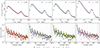 |
Fig. 1. Top panels: 2PCF measurements for four comoving snapshots from the Flagship I simulation of the Model 3 HOD. Bottom panels: Same but for the 3PCF measurements. The triangular configurations are ordered by increasing values of r12, r13, and r23 under the condition r12 ≤ r13 ≤ r23, as depicted in Fig. A.1. The circles are colour-coded according to the η, while the vertical grey lines mark a group of triangles that share the same value of the smaller side (r12). |
The Landy–Szalay estimator for the 2PCF can be easily extended to the analogous estimator for the 3PCF, constructed in terms of triplet counts (see e.g. Szapudi & Szalay 1998). However, since such an estimator scales with the number of galaxies Ng as 𝒪(Ng3), its computational cost quickly becomes prohibitive when it comes to very large datasets such as those we considered here, where Ng is around 108. To resolve this issue, Slepian & Eisenstein (2015) introduced an estimator based on the spherical harmonics decomposition (SHD), which improves significantly the computational efficiency. In this approach, the dependence of the 3PCF on the angle between the triangle sides r12 and r13 is expanded in terms of Legendre polynomials according to Eq. (10). As a result, the full estimator  is written as a function of an estimator
  of the expansion coefficients as
 (38)
(38)
thereby reducing the computational complexity to 𝒪(Ng2). The coefficients are estimated as
 (39)
(39)
where NDDD, ℓ, NDDR, ℓ, NDRR, ℓ, and NDRR, ℓ are, in turn, the coefficients of the Legendre expansion of the triplets counts from the galaxy catalogue, from the random and the two mixed terms, directly evaluated in the approach of Slepian & Eisenstein (2015). Again, since we are working with a simulation box with periodic boundary conditions, it is possible to simplify the evaluation of the coefficients  and derive an analytical expression for the monopole of the random triplet counts NRRR, 0.
The SHD estimator is known to be less efficient for isosceles or nearly isosceles triangle configurations (i.e. with r12 ≃ r13). In these cases, a large value of ℓmax is required to recover results consistent with those of the standard, direct-counting, estimator. Indeed, for isosceles triangles each coefficient of the expansion in Eq. (10) is the result of an integration over the bispectrum down to small, non-linear scales, beyond the range of validity of the perturbative model. On the other hand, using a fixed ℓmax ensures internal consistency between measurements and theory. To mitigate this issue, we introduced the quantity (see e.g. Veropalumbo et al. 2022)
 (40)
(40)
with Δr being the separation bin size, to parametrise the proximity of a given configuration to the isosceles case. Fixing a lower limit (ηmin) amounts to excluding isosceles, or nearly isosceles configurations.
In the bottom panels of Fig. 1 we present the 3PCF measurements for the four snapshots. The triangle index is defined by increasing value of r12, r13, and r23 under the condition r12 ≤ r13 ≤ r23, as depicted in Fig. A.1. The measurements include all configurations with side lengths from rmin = 0 h−1 Mpc to rmax = 150 h−1 Mpc in bins of width Δr = 5 h−1 Mpc. We expanded the 3PCF up to ℓmax = 10, which strikes an ideal balance between computational efficiency and information content. A more detailed description of the numerical implementation and validation of the SHD estimator for the 3PCF will be given in Euclid Collaboration: Veropalumbo et al. (in prep.), while a similar presentation of the 2PCF estimator is given in Euclid Collaboration: de la Torre et al. (2025).
4.3. Covariance
We made use of a covariance matrix obtained from an analytical model for both two- and three-point functions. We worked in the Gaussian approximation, so all covariance depends simply on the galaxy power spectrum, and we further assumed a linear model for this spectrum.
For the 2PCF covariance we have (Grieb et al. 2016; Lippich et al. 2019)
 (41)
(41)
where V is the box volume,  are the bin-averaged, zeroth-order Bessel functions (see Eq. A19 in Grieb et al. 2016), while
 (42)
(42)
is the linear galaxy power spectrum including a Poisson shot-noise contribution,  being the galaxy number density. For each redshift snapshot, we computed the covariance matrix using the bias and density values listed in Table 2. As noted by Smith (2009), a more detailed treatment of discrete tracers introduces additional terms in the covariance – particularly relevant at low number density – even under Gaussian assumptions. These include contributions from combinatoric sampling effects, which are not included in our model; this is sufficient given the number density of the simulated dataset.
For the 3PCF covariance, we followed the expression proposed in Slepian & Eisenstein (2015), rigorously validated in Veropalumbo et al. (2022). This again takes advantage of the SHD writing the covariance between two measurements  and
and  as
as
 (43)
(43)
where 𝒞ζ, ℓℓ′(r12, r13; r′12, r′13) represents the covariance between the coefficients  and
and  . This, in turn, is given by
![Mathematical equation: $$ \begin{aligned} \mathcal{C} _{\zeta ,\ell \ell \prime }&(r_i, r_j;r\prime _i, r\prime _j )= \\ \nonumber =&\frac{(2\ell +1)\, (2\ell \prime +1)\, (-1)^{\ell +\ell \prime }}{(2\pi )^6\,V}\!\int \!{\mathrm{d} } p_1 \, {\mathrm{d} } p_2 \, {\mathrm{d} } p_3 \, \delta _{\rm {D}}(\mathbf p _{123}) \\ \nonumber&\times P_{\rm {tot}}(p_1) \, P_{\rm {tot}}(p_2) \, P_{\rm {tot}}(p_3) \bar{j}_\ell (p_1r_i) \, \bar{j}_\ell (p_2r_j) \, {\mathcal{L} }_\ell (\mu _{12}) \\ \nonumber&\times \left[\bar{j}_{\ell \prime }(p_1r_i\prime ) \, \bar{j}_{\ell \prime }(p_2r_j\prime ) \, {\mathcal{L} }_{\ell \prime }(\mu _{12})+5\ \mathrm{{perm}.}\right]. \end{aligned} $$](/articles/aa/full_html/2026/03/aa56177-25/aa56177-25-eq56.gif) (44)
(44)
We refer the reader to Slepian & Eisenstein (2015) for a detailed description of the practical evaluation of this expression.
In the Gaussian approximation, the cross-covariance between the two- and three-point functions vanishes, as the only contributions arise from the bispectrum of the density field and the connected 5-point function (see e.g. Sefusatti et al. 2006). While these terms are expected to introduce non-negligible correlations – potentially at the ∼20% level for amplitude-related parameters – we neglected them in this work for consistency with the Gaussian covariance framework. This choice is justified by the scope of our analysis, which focuses on validating the modelling pipeline rather than delivering optimal cosmological constraints.
5. Likelihood analysis and performance metrics
We define in the section the likelihood function we adopted to fit the parameters of our model to the simulation measurements. We also introduce the statistical tools we used to determine the range of validity of the model in terms of the GoF, the level of theoretical uncertainties introduced by the model, and the ability to constrain cosmological parameters.
5.1. Likelihood function
We adopted a Gaussian likelihood function for both the 2PCF and the 3PCF measurements. We thus have
 (45)
(45)
where vector θ denotes the model parameters while the χ2 for the 2PCF is given by
![Mathematical equation: $$ \begin{aligned} \chi ^2_{\rm \xi }(\mathbf {\theta} ) = \sum _{i,j=1}^{N_{r}} \big [ \xi _i(\mathbf {\theta} ) - \hat{\xi }_i \big ] \ C^{-1}_{\xi , ij} \ \big [ \xi _j(\mathbf {\theta} ) - \hat{\xi }_j \big ], \end{aligned} $$](/articles/aa/full_html/2026/03/aa56177-25/aa56177-25-eq58.gif) (46)
(46)
with ξ(θ) and  representing respectively the 2PCF theoretical prediction and its measurements and with the sum running over the separation bins ri and rj, Nr being the total number of bins, corresponding to the size of the data vector. Similarly, for the 3PCF we have
 (47)
(47)
with
![Mathematical equation: $$ \begin{aligned} \chi ^2_{\zeta }(\mathbf {\theta} ) = \sum _{i,j=1}^{N_{\rm t}} \big [ \zeta _i(\mathbf {\theta} ) - \hat{\zeta }_i \big ] \ C^{-1}_{\zeta , ij} \ \big [ \zeta _j(\mathbf {\theta} ) - \hat{\zeta }_j \big ], \end{aligned} $$](/articles/aa/full_html/2026/03/aa56177-25/aa56177-25-eq61.gif) (48)
(48)
with the sum now extending over all triangular configuration up to their total number (Nt).
The likelihood of joint measurements of the 2PCF and 3PCF is simply given by
 (49)
(49)
and, correspondingly, the joint χ2 will be
 (50)
(50)
since, as mentioned above, we neglected the cross-covariance between the two statistics.
We sampled the posterior using the emcee code2 (Foreman-Mackey et al. 2013), implementing an affine-invariant ensemble sampler, which is particularly well suited to high-dimensional parameter spaces. We employed 50 walkers in each run and ensured that the chains are terminated only after exceeding 100 integrated autocorrelation times, thereby ensuring full convergence.
The model parameters, along with uniform priors assumed in all likelihood evaluations, are outlined in Table 3. The choice of large intervals is meant to ensure uninformative priors.
Cosmological and nuisance parameters of the 2PCF and 3PCF models.
5.2. Performance metrics
Our main goal is the assessment of the range of validity of the model, determining the minimum scale, rmin, down to which the model can still accurately describe the measurements without introducing significant systematic uncertainties to the recovered cosmological parameters. As in the companion paper (Euclid Collaboration: Pezzotta et al. 2024), this task is carried out using three performance metrics: a GoF, a figure of bias (FoB), and figure of merit (FoM) as defined below.
5.2.1. Goodness of fit
For an assessment on the GoF, we simply used the standard χ2 test. The χ2 definitions for the 2PCF, 3PCF, and joint at a given point θ in the parameter space are given in Eqs. (46), (48), and (50). The posterior-averaged value, ⟨χ2⟩post, is then compared to the thresholds from the χ2 distribution at the 68% and 95% confidence levels, determined in terms of the appropriate number of degrees of freedom, computed as the difference between the size of the data vector and the number of model parameters.
5.2.2. Figure of bias
We quantified the uncertainties in recovering a subset of fiducial, cosmological parameters (θfid) due to model systematic uncertainties in terms of an FoB defined as
![Mathematical equation: $$ \begin{aligned} \mathrm{{FoB}}(\mathbf {\theta} ) = \left[ \left( \langle \mathbf {\theta} \rangle _{\rm {post}} - \mathbf {\theta} _{\rm {fid}} \right)^\mathrm{T} S^{-1}(\mathbf {\theta} ) \left( \langle \mathbf {\theta} \rangle _{\rm {post}} - \mathbf {\theta} _{\rm {fid}} \right) \right]^{1/2}, \end{aligned} $$](/articles/aa/full_html/2026/03/aa56177-25/aa56177-25-eq64.gif) (51)
(51)
where ⟨θ⟩post represents the parameter averaged over the posterior distribution, while S(θ) is the parameters’ covariance matrix, evaluated from the same posterior distribution.
When θ consists of a single parameter, the FoB measures the deviation of the posterior mean from the fiducial value in units of the parameter’s standard deviation, with FoB values of one and two corresponding to the 68% and 95% confidence levels, respectively. However, when dealing with multiple parameters, these thresholds must be recalculated by integrating a multivariate normal distribution over the appropriate number of dimensions. For instance, in the case of three parameters relevant for the results of Sect. 7, the 68% and 95% confidence levels correspond to FoB values of 1.87 and 2.80, respectively.
5.2.3. Figure of merit
Finally, we defined an FoM (Albrecht et al. 2006; Wang 2008) to quantify the constraining power of our model over a specific range of scales and under given bias assumptions:
![Mathematical equation: $$ \begin{aligned} \mathrm{{FoM}}(\mathbf {\theta} ) = \frac{1}{\sqrt{\det [S(\mathbf {\theta} )]}} , \end{aligned} $$](/articles/aa/full_html/2026/03/aa56177-25/aa56177-25-eq65.gif) (52)
(52)
where det[S(θ)] is the determinant of the covariance matrix of the parameters of interest. This represents the hyper-volume enclosed by the hyper-surface defined by the covariance matrix S(θ). Therefore, a larger FoM indicates tighter constraints on the model parameters.
6. Galaxy bias
In this section we assess the range of validity of our bias model for both the 2PCF and 3PCF. Our focus will be then on the GoF test, keeping fixed the cosmological parameters at their fiducial values. We considered both the case where all bias parameters are free and the case where the bias relations mentioned above is assumed to reduce the parameter space. We also needed to make sure that no significant running of the bias parameters was present, i.e. there was no significant variation in the recovered parameters, as a function of the minimal scale defining the data vectors.
6.1. Maximal model
We started with the maximal model (see e.g. Oddo et al. 2021), with all bias parameters free, with the priors given in Table 3. In Fig. 2 we show the χ2 averaged over the posterior distribution for the four redshift snapshots and for the 2PCF, 3PCF, and joint 2PCF+3PCF data vector.
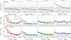 |
Fig. 2. GoF test for the bias 2PCF and 3PCF models with fixed cosmological parameters as a function of the minimal scale, |


We notice in the first place that while the one-loop 2PCF model provides a good fit for all scales considered, the tree-level 3PCF prediction fails for separations below 20 h−1 Mpc at z = 0.9, with a better performance at higher redshift. Under the choice of ηmin = 1, Eq. (40), including configurations closer to the isosceles case, the validity of the model is further restricted to rmin > 20 h−1 Mpc at z = 0.9 and rmin > 10 h−1 Mpc for z = 1.2 and above.
In Fig. 3 we show the marginalised 2D constraints on the nuisance parameters (bias and counter-term) from the 2PCF analysis against the joint 2PCF plus 3PCF analysis for several values of  . This shows in the first place the peculiar and significant constraining power of higher-order statistics on linear and non-linear bias. This is particularly evident in the reduction of the posterior uncertainty on the non-linear parameter b2 and non-local parameters b𝒢2 and bΓ3. It further shows that down to
  no running of the bias parameter is evident, with all analyses at different rmin consistently reducing the posterior uncertainty.
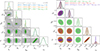 |
Fig. 3. Left panel: Marginalised 2D constraints at confidence intervals of 68.3% and 99.5%, on the nuisance parameters (bias and counter-term) from the 2PCF analysis (grey shaded areas) against the joint 2PCF and 3PCF analysis for several values of |


The plots include, as a vertical grey band, an estimate of the value of the linear bias b1 obtained from a comparison of the galaxy power spectrum with measurements of the matter power spectrum in Euclid Collaboration: Pezzotta et al. (2024). We find that the inclusion of the 3PCF consistently yields posterior distributions for b1 that are visually closer to the reference value across all the minimum scale cuts explored. While the 2PCF-only results remain statistically consistent, they exhibit broader posteriors, reflecting a stronger degeneracy with other model parameters. We revisit this aspect in the context of cosmological parameter constraints in the following section.
6.2. Bias relations
The right panel of Fig. 3 shows the same results for the joint analysis with rmin = 30 h−1 Mpc and ηmin = 3 (green contours), here compared to the same set-up but with the additional assumptions of two bias relations. We considered, in particular, the b𝒢2(b1) relation alone, Eq. (16), (red contours) and its combination with the relation for bΓ3 of Eq. (17). We display only the results for the z = 1.5 snapshots, noticing that for the measurements at other redshifts we obtain qualitatively similar results.
We notice that in both cases, the bias relations provide a reduction of the parameter space by one and two parameters, respectively, without affecting the b1, b2 constraints. On this specific contour in fact we do not observe any induced systematic shift as we do not notice any appreciable reduction in the uncertainty. This is noticeable instead on the c0 parameter, describing the combined effect of the EFT counter-term and higher derivative bias. These results provide some evidence that the bias relations can be used to speed up the likelihood evaluation without compromising the main results. We return to this point when discussing cosmological parameters constraints.
We close the section by noticing that the adoption of one or two bias relations does not lead to any worsening of the GoF, in terms of the χ2 test. We avoid a dedicated figure since the difference with the maximal model case would be barely visible.
7. Cosmological parameters from the joint, full-shape analysis
In this section we present the results for the full-shape, joint analysis of 2PCF and 3PCF aiming at constraining three cosmological parameters: the amplitude of scalar fluctuations (As), the CDM density (ωcdm), and the Hubble constant (h). This minimal set captures the main physical effects to which large-scale structure observables are directly sensitive: As determines the amplitude of fluctuations and is probed by the power spectrum and bispectrum; ωcdm governs the growth history and the shape of the clustering signal; and h fixes the physical scales through the matter–radiation equality scale and the sound horizon, affecting the shape of correlation functions in real space. Limiting our analysis to these parameters highlights the constraining power of the full-shape information.
To the best of our knowledge, this is the first attempt at estimating the improvement due to adding the 3PCF to the full-shape analysis of the 2PCF, although still limited to real space. Until now, 3PCF analyses have been restricted to template fitting, i.e. using fixed-shape models to extract cosmological information from the BAO scale position or from the anisotropy induced by redshift-space distortions, rather than performing full-shape parameter inference, due to the considerable computational demands of a full cosmology-dependent 3PCF model.
A key ingredient, to achieve this goal, is the emulator described in Appendix B. Constructed using a PyTorch3 framework, the emulator has undergone extensive testing and has been fully integrated into the same sampler. The emulator extends to the 2PCF prediction, further enhancing the overall efficiency of our analysis.
Figure 4 shows marginalised constraints on cosmological parameters As, ωcdm, h, and on the linear bias b1 derived from the joint 2PCF and 3PCF analysis as a function of the minimal scale rmin that characterises the 3PCF data vector, with the minimal separation in the 2PCF measurements fixed at  . The four columns span the different redshifts. As in Fig. 2, varying shades of these colours correspond to different choices for the parameter ηmin. The dashed black lines denote the fiducial values assumed for the simulations, together with the grey line that shows the same fiducial values for b1 considered in Fig. 3. Overall, the results show good agreement between the emulated predictions and the expected values. For large values of rmin, the estimates for As and b1 tend to deviate further from the expected values, largely due to projection effects caused by a large degeneracy between these parameters. On the other hand, moving to the small-scale regime, a possible failure of the model to recover the fiducial values is only evident for ωcdm at the lowest redshift of z = 0.9. Below rmin = 40 h−1 Mpc, the estimates for As and b1(z) exhibit a slight dependence on the choice of ηmin, with the case of ηmin = 1 leading to more biased values for these parameters, particularly at low redshift.
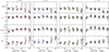 |
Fig. 4. Marginalised constraints on the cosmological parameters and linear bias from a joint 2PCF and 3PCF analysis. The posterior mean along with its uncertainties is displayed as a function of the minimal scale ( |


In Fig. 5 we present the performance metrics corresponding to the results of Fig. 4, all as a function of the minimal scales  , with
  fixed at 25 h−1 Mpc, and for the same three different values of ηmin. The top panels show the posterior-averaged ⟨χ2⟩post. The grey bands denote the 68% and 99.7% confidence levels for the χ2 distribution. We find a good fit for
  except for the lowest redshift where
  ensures a safer result. This is naturally consistent with the results at fixed cosmology. The middle panels show the FoB, defined in terms of the parameters As, ωcdm, and h. The uncertainties are shown again in two shades of grey, corresponding to 68% and 95% confidence levels. The model provides overall unbiased results except for the first separation bin at rmin = 10 h−1 Mpc, for all redshifts and for all values of ηmin. Finally, the bottom panels of Fig. 5 show the FoM, defined again in terms of the three cosmological parameters. The FoM increases significantly across the whole separation range (notice the log-scale on the y-axis) and presents also larger values in the lowest redshift snapshots. In addition, the choice of a low value for ηmin can also make a large difference, since this increase the size of the data vector and relative S/N.
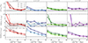 |
Fig. 5. Performance metrics for the full-shape, joint analysis of the 2PCF and the 3PCF. All quantities are shown as a function of the minimal scale ( |


The left plot of Fig. 6 shows the constraints on the cosmological parameters at z = 0.9 plus the linear bias obtained from the combined statistics for different choices of  and ηmin, compared to the 2PCF-only constraints where we include an additional, informative Gaussian prior on b1 for illustrative purposes defined by a 10% error on the best-fit value obtained from the joint analysis. This is required by the strong degeneracy between As and b1 in the 2PCF likelihood. This degeneracy is still present in the joint analysis, although significantly reduced without imposing any prior on b1. We obtain a discrepancy with the fiducial value of As at confidence interval of 68.3% for the configuration with
  and ηmin = 2, while the discrepancy is smaller for the other parameters, despite the additional degeneracy between h and ωcdm. Interestingly, no tension is visible on the h and ωcdm constraints.
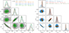 |
Fig. 6. Left panel: Marginalised 2D and 1D posterior distributions at z = 0.9 from the joint 2PCF and 3PCF analysis of the cosmological parameters h, ωcdm, and As and the linear bias parameter b1 for various 3PCF scale cuts ( |


The same results are found with no relevant difference for all snapshots, as described in Fig. C.1. We remind the reader that the posterior distributions are not statistically independent since each realisation is a different snapshot of the same evolving dark matter perturbations, sharing the same initial seeds. We observe that at lower redshifts the constraints are tighter due to the larger density of the galaxy distribution and that, in general, both h and ωcdm exhibit accurate estimates of the fiducial values. The largest discrepancy, at the limit of the confidence interval of 99.5% contour, is obtained for As at z = 1.2. We notice that now also the linear bias parameter is correctly recovered at all redshifts.
In the right plot of Fig. 6, we compare the maximal model with all free parameters, assuming  and ηmin = 3, to the results obtained assuming the bias relation of Eq. (16) for
  , and its combination with the relation for bΓ3 of Eq. (17), showing the same set of parameters as in the right plot. Overall, we notice how the adoption of the bias relations enhances the precision of the cosmological parameter constraints. Notably, the 2D posterior distribution of As and b1, affected by a strong degeneracy, benefits the most from this additional information, although, again, we notice a slightly biased estimate for As. As presented in Fig. C.2, which shows the full set of parameters, the bΓ3 relation greatly reduces the uncertainty on the higher derivatives and/or counter-term parameter c0, as in the bias-only case.
8. Conclusions
In this work we provide a validation of PT models for the 2PCF and 3PCF in real space across a redshift range and against a synthetic galaxy catalogue representative of the Euclid spectroscopic galaxy survey (see e.g. Euclid Collaboration: Mellier et al. 2025).
We took advantage of galaxy clustering measurements obtained from four redshift snapshots of the Flagship I simulation populated with the HOD following the Model 3 prescription of Pozzetti et al. (2016). In particular, we determined HOD parameters by selecting galaxies with a Hα flux limit of fHα = 2 × 10⁻¹⁶ erg cm−2 s−1. The 3PCF measurements in particular, presented in Sect. 4, are based on the SHD introduced by Slepian & Eisenstein (2015); see also Euclid Collaboration: Veropalumbo et al. (in prep). This estimator allowed us to measure all 3PCF configurations while keeping a manageable computational cost.
The galaxy 2PCF is modelled at the NLO within the framework of EFTofLSS, involving up to five nuisance parameters: b1, b2, b𝒢2, bΓ3, and the parameter c0, which describes an EFT counter-term and higher-derivative bias. The 3PCF, on the other hand, was modelled at the LO in PT, with the tree-level expression depending only on the bias parameters b1, b2, and b𝒢2.
We first assessed the GoF provided by the model via a χ2 test and explored its range of validity as a function of the minimal scale included in the data vector and of the additional parameter ηmin Eq. (40), progressively excluding nearly isosceles triangles from the analysis (Sect. 6). The predictions for these configurations are, in fact, affected by systematic uncertainties when the Legendre expansion of Eq. (10) is limited to a relatively small number of multipoles, as in any practical application. We find that the tree-level model for the 3PCF fails below separations of 20 h−1 Mpc when ηmin ≥ 2, while a larger minimum scale should be considered for when ηmin = 1. Commonly adopted relations between bias parameters, such as those for b𝒢2(b1) and bΓ3(b1), can help reduce the parameter space without affecting the determination of the other bias parameters, except for the c0 parameter.
The main results of the paper, presented in Sect. 7, are from a joint, full-shape analysis of the 2PCF and 3PCF, carried out with the aim of constraining three cosmological parameters: As, ωcdm, and h. Cosmological analyses involving the 3PCF have so far been based on template fitting (see e.g. Slepian et al. 2017; Slepian & Eisenstein 2018; Veropalumbo et al. 2021; Sugiyama et al. 2021; Farina et al. 2026), as a direct evaluation of the 3PCF model is computationally too expensive. To overcome this hurdle, we developed an emulator able to provide fast and accurate full predictions for both 2PCF and 3PCF, thereby enabling a complete joint analysis of the two statistics.
In this case, in addition to the χ2 test, we adopted an FoB and an FoM to quantify the model’s systematic uncertainties along with its ability to constrain cosmological parameters. Focusing only on the results for the joint analysis, since only this configuration allows us to properly constrain all three parameters without informative priors, we find that a conservative choice for the scale cuts is given by  and ηmin = 3. A more aggressive configuration with
  and ηmin = 2 is still acceptable, although a tension at the confidence interval of 68.3% with the fiducial value As begins to show. This finding aligns with conclusions drawn from previous methodological studies on the galaxy bias model (see e.g. Veropalumbo et al. 2022, for further details). On the other hand, selecting ηmin = 1 led to more unstable results, particularly at lower redshifts.
Adopting bias relations provides only a limited advantage in a bias-only analysis. However, when cosmological parameters are included, it can lead to tighter constraints, most notably on As, particularly in the case of Eq. (16).
In conclusion, we confirm that, as expected, the combination of 2PCF and 3PCF in real space provides greater constraining power with respect to the 2PCF alone, effectively breaking the degeneracy between As and b1(z). We also expect the improvement to be less pronounced in redshift space, where the 2PCF multipoles typically show reduced degeneracies among cosmological and bias parameters. This work represents a first step towards a full-shape joint analysis in redshift space that, out of necessity, will require tools such as the emulator developed here. In this perspective, this study paves the way for the application of emulated predictions in comparisons to real data, setting the stage for a complete analysis of galaxy clustering data in configuration space that will be on the same footing as power spectrum and bispectrum joint analyses.
This work is part of a series of preparation papers aimed at validating theoretical models for the analysis of galaxy clustering statistics from the Euclid spectroscopic sample. A first assessment of the real-space model for the galaxy power spectrum has been presented in Euclid Collaboration: Pezzotta et al. (2024). The cases of the redshift space power spectrum and 2PCF will be presented respectively in Euclid Collaboration: Camacho et al. (in prep.) and Euclid Collaboration: Kärcher et al. (in prep.). In addition, the redshift-space, joint power spectrum and bispectrum, and 2PCF-3PCF cases will appear in Euclid Collaboration: Pardede et al. (in prep.) and Euclid Collaboration: Pugno et al. (in prep.). Finally, another study will explore the BAO signal in the redshift-space 3PCF.
Acknowledgments
We thank Krister Nagainis, Adi Nusser and Andrea Enia for useful discussions. MG and MM acknowledge support from the research grant ‘Optimizing the extraction of cosmological information from Large Scale Structure analysis in view of the next large spectroscopic surveys’ from MIUR, PRIN 2022 (grant 2022NY2ZRS 001). MM acknowledges the financial contribution from the grant ASI n. 2024-10-HH.0 “Attività scientifiche per la missione Euclid – fase E. The Euclid Consortium acknowledges the European Space Agency and a number of agencies and institutes that have supported the development of Euclid, in particular the Agenzia Spaziale Italiana, the Austrian Forschungsförderungsgesellschaft funded through BMK, the Belgian Science Policy, the Canadian Euclid Consortium, the Deutsches Zentrum für Luft- und Raumfahrt, the DTU Space and the Niels Bohr Institute in Denmark, the French Centre National d’Etudes Spatiales, the Fundação para a Ciência e a Tecnologia, the Hungarian Academy of Sciences, the Ministerio de Ciencia, Innovación y Universidades, the National Aeronautics and Space Administration, the National Astronomical Observatory of Japan, the Netherlandse Onderzoekschool Voor Astronomie, the Norwegian Space Agency, the Research Council of Finland, the Romanian Space Agency, the State Secretariat for Education, Research, and Innovation (SERI) at the Swiss Space Office (SSO), and the United Kingdom Space Agency. A complete and detailed list is available on the Euclid web site (www.euclid-ec.org).
References
- Adame, A. G., Aguilar, J., Ahlen, S., et al. 2025, JCAP, 02, 021 [CrossRef] [Google Scholar]
- Albrecht, A., Bernstein, G., Cahn, R., et al. 2006, arXiv e-prints [arXiv:astro-ph/0609591] [Google Scholar]
- Assassi, V., Baumann, D., Green, D., & Zaldarriaga, M. 2014, JCAP, 08, 056 [CrossRef] [Google Scholar]
- Baldauf, T., Seljak, U., Desjacques, V., & McDonald, P. 2012, Phys. Rev. D, 86, 083540 [NASA ADS] [CrossRef] [Google Scholar]
- Baldauf, T., Mirbabayi, M., Simonović, M., & Zaldarriaga, M. 2015, Phys. Rev. D, 92, 043514 [NASA ADS] [CrossRef] [Google Scholar]
- Bardeen, J. M., Bond, J. R., Kaiser, N., & Szalay, A. S. 1986, ApJ, 304, 15 [Google Scholar]
- Baumann, D., Nicolis, A., Senatore, L., & Zaldarriaga, M. 2012, JCAP, 07, 051 [CrossRef] [Google Scholar]
- Bernardeau, F., Colombi, S., Gaztañaga, E., & Scoccimarro, R. 2002, Phys. Rep., 367, 1 [Google Scholar]
- Beutler, F., Seo, H.-J., Saito, S., et al. 2017, MNRAS, 466, 2242 [Google Scholar]
- Blas, D., Garny, M., Ivanov, M. M., & Sibiryakov, S. 2016a, JCAP, 07, 052 [Google Scholar]
- Blas, D., Garny, M., Ivanov, M. M., & Sibiryakov, S. 2016b, JCAP, 07, 028 [CrossRef] [Google Scholar]
- Cabass, G., Ivanov, M. M., Philcox, O. H. E., Simonović, M., & Zaldarriaga, M. 2022, Phys. Rev. Lett., 129, 021301 [Google Scholar]
- Carrasco, J. J. M., Hertzberg, M. P., & Senatore, L. 2012, J. High Energy Phys., 9, 82 [Google Scholar]
- Catelan, P., Lucchin, F., Matarrese, S., & Porciani, C. 1998, MNRAS, 297, 692 [CrossRef] [Google Scholar]
- Chan, K. C., Scoccimarro, R., & Sheth, R. K. 2012, Phys. Rev. D, 85, 083509 [CrossRef] [Google Scholar]
- Coles, P., Moscardini, L., Lucchin, F., Matarrese, S., & Messina, A. 1993, MNRAS, 264, 749 [Google Scholar]
- Crocce, M., & Scoccimarro, R. 2008, Phys. Rev. D, 77, 023533 [NASA ADS] [CrossRef] [Google Scholar]
- D’Amico, G., Gleyzes, J., Kokron, N., et al. 2020, JCAP, 05, 005 [Google Scholar]
- D’Amico, G., Lewandowski, M., Senatore, L., & Zhang, P. 2025, Phys. Rev. D, 111, 063514 [Google Scholar]
- Dawson, K. S., Schlegel, D. J., Ahn, C. P., et al. 2013, AJ, 145, 10 [Google Scholar]
- DESI Collaboration (Aghamousa, A., et al.) 2016, arXiv e-prints [arXiv:1611.00036] [Google Scholar]
- Desjacques, V. 2008, Phys. Rev. D, 78, 103503 [CrossRef] [Google Scholar]
- Desjacques, V., Crocce, M., Scoccimarro, R., & Sheth, R. K. 2010, Phys. Rev. D, 82, 103529 [CrossRef] [Google Scholar]
- Desjacques, V., Jeong, D., & Schmidt, F. 2018, Phys. Rep., 733, 1 [Google Scholar]
- Dore, O., Hirata, C., Wang, Y., et al. 2019, BAAS, 51, 341 [Google Scholar]
- Eggemeier, A., Scoccimarro, R., & Smith, R. E. 2019, Phys. Rev. D, 99, 123514 [NASA ADS] [CrossRef] [Google Scholar]
- Eggemeier, A., Scoccimarro, R., Crocce, M., Pezzotta, A., & Sánchez, A. G. 2020, Phys. Rev. D, 102, 103530 [NASA ADS] [CrossRef] [Google Scholar]
- Eisenstein, D. J., Zehavi, I., Hogg, D. W., et al. 2005, ApJ, 633, 560 [Google Scholar]
- Eisenstein, D. J., Seo, H.-J., & White, M. 2007, ApJ, 664, 660 [Google Scholar]
- Euclid Collaboration (Blanchard, A., et al.) 2020, A&A, 642, A191 [NASA ADS] [CrossRef] [EDP Sciences] [Google Scholar]
- Euclid Collaboration (Scaramella, R., et al.) 2022, A&A, 662, A112 [NASA ADS] [CrossRef] [EDP Sciences] [Google Scholar]
- Euclid Collaboration (Pezzotta, A., et al.) 2024, A&A, 687, A216 [Google Scholar]
- Euclid Collaboration (de la Torre, S., et al.) 2025, A&A, 700, A78 [Google Scholar]
- Euclid Collaboration (Mellier, Y., et al.) 2025, A&A, 697, A1 [Google Scholar]
- Euclid Collaboration (Risso, I., et al.) 2026, A&A, 707, A233 [Google Scholar]
- Fang, X., Eifler, T., & Krause, E. 2020, MNRAS, 497, 2699 [NASA ADS] [CrossRef] [Google Scholar]
- Farina, A., Veropalumbo, A., Branchini, E., & Guidi, M. 2026, J. Cosmol. Astropart. Phys., 2026, 028 [Google Scholar]
- Foreman-Mackey, D., Hogg, D. W., Lang, D., & Goodman, J. 2013, PASP, 125, 306 [Google Scholar]
- Frieman, J. A., & Gaztanaga, E. 1994, ApJ, 425, 392 [Google Scholar]
- Fry, J. N. 1984, ApJ, 279, 499 [NASA ADS] [CrossRef] [Google Scholar]
- Fry, J. N. 1994, Phys. Rev. Lett., 73, 215 [Google Scholar]
- Fry, J. N., & Gaztañaga, E. 1993, ApJ, 413, 447 [NASA ADS] [CrossRef] [Google Scholar]
- Fujita, T., Mauerhofer, V., Senatore, L., Vlah, Z., & Angulo, R. 2020, JCAP, 01, 009 [CrossRef] [Google Scholar]
- Gaztañaga, E., Norberg, P., Baugh, C. M., & Croton, D. J. 2005, MNRAS, 364, 620 [Google Scholar]
- Gaztañaga, E., Cabré, A., Castander, F., Crocce, M., & Fosalba, P. 2009, MNRAS, 399, 801 [Google Scholar]
- Gil-Marín, H., Percival, W. J., Verde, L., et al. 2017, MNRAS, 465, 1757 [Google Scholar]
- Grieb, J. N., Sánchez, A. G., Salazar-Albornoz, S., & Dalla Vecchia, C. 2016, MNRAS, 457, 1577 [NASA ADS] [CrossRef] [Google Scholar]
- Grieb, J. N., Sánchez, A. G., Salazar-Albornoz, S., et al. 2017, MNRAS, 467, 2085 [NASA ADS] [Google Scholar]
- Guidi, M., Veropalumbo, A., Branchini, E., Eggemeier, A., & Carbone, C. 2023, JCAP, 08, 066 [Google Scholar]
- Guzzo, L., Pierleoni, M., Meneux, B., et al. 2008, Nature, 451, 541 [Google Scholar]
- Hamilton, A. J. S. 2000, MNRAS, 312, 257 [NASA ADS] [CrossRef] [Google Scholar]
- Hivon, E., Bouchet, F. R., Colombi, S., & Juszkiewicz, R. 1995, A&A, 298, 643 [Google Scholar]
- Hou, J., Sánchez, A. G., Scoccimarro, R., et al. 2018, MNRAS, 480, 2521 [NASA ADS] [CrossRef] [Google Scholar]
- Ivanov, M. M., & Sibiryakov, S. 2018, JCAP, 07, 053 [Google Scholar]
- Ivanov, M. M., Simonović, M., & Zaldarriaga, M. 2020, JCAP, 05, 042 [CrossRef] [Google Scholar]
- Ivezic, Z., Tyson, J. A., Axelrod, T., et al. 2009, Am. Astron. Soc. Meeting Abstr., 213, 460.03 [Google Scholar]
- Jing, Y. P., & Börner, G. 2004, ApJ, 607, 140 [Google Scholar]
- Kaiser, N. 1984, ApJ, 284, L9 [NASA ADS] [CrossRef] [Google Scholar]
- Landy, S. D., & Szalay, A. S. 1993, ApJ, 412, 64 [Google Scholar]
- Laureijs, R., Amiaux, J., Arduini, S., et al. 2011, arXiv e-prints [arXiv:1110.3193] [Google Scholar]
- Lazeyras, T., Wagner, C., Baldauf, T., & Schmidt, F. 2016, JCAP, 02, 018 [Google Scholar]
- Lippich, M., Sánchez, A. G., Colavincenzo, M., et al. 2019, MNRAS, 482, 1786 [NASA ADS] [CrossRef] [Google Scholar]
- Marín, F. 2011, ApJ, 737, 97 [Google Scholar]
- Marín, F. A., Blake, C., Poole, G. B., et al. 2013, MNRAS, 432, 2654 [Google Scholar]
- Matsubara, T. 2008, Phys. Rev. D, 77, 063530 [NASA ADS] [CrossRef] [Google Scholar]
- McBride, C. K., Connolly, A. J., Gardner, J. P., et al. 2011, ApJ, 739, 85 [Google Scholar]
- McDonald, P. 2006, Phys. Rev. D, 74, 103512 [CrossRef] [Google Scholar]
- McDonald, P., & Roy, A. 2009, JCAP, 08, 020 [CrossRef] [Google Scholar]
- Moresco, M., Marulli, F., Moscardini, L., et al. 2017, A&A, 604, A133 [NASA ADS] [CrossRef] [EDP Sciences] [Google Scholar]
- Moresco, M., Veropalumbo, A., Marulli, F., Moscardini, L., & Cimatti, A. 2021, ApJ, 919, 144 [NASA ADS] [CrossRef] [Google Scholar]
- Oddo, A., Rizzo, F., Sefusatti, E., Porciani, C., & Monaco, P. 2021, JCAP, 11, 038 [CrossRef] [Google Scholar]
- Peacock, J. A., Cole, S., Norberg, P., et al. 2001, Nature, 410, 169 [Google Scholar]
- Peebles, P. J. E. 1973, ApJ, 185, 413 [Google Scholar]
- Percival, W. J., Cole, S., Eisenstein, D. J., et al. 2007, MNRAS, 381, 1053 [Google Scholar]
- Pezzotta, A., de la Torre, S., Bel, J., et al. 2017, A&A, 604, A33 [NASA ADS] [CrossRef] [EDP Sciences] [Google Scholar]
- Philcox, O. H. E., & Ivanov, M. M. 2022, Phys. Rev. D, 105, 043517 [CrossRef] [Google Scholar]
- Potter, D., Stadel, J., & Teyssier, R. 2017, Comput. Astrophys. Cosmol., 4, 2 [NASA ADS] [CrossRef] [Google Scholar]
- Pozzetti, L., Hirata, C. M., Geach, J. E., et al. 2016, A&A, 590, A3 [NASA ADS] [CrossRef] [EDP Sciences] [Google Scholar]
- Pugno, A., Eggemeier, A., Porciani, C., & Kuruvilla, J. 2025, JCAP, 01, 075 [Google Scholar]
- Sánchez, A. G., Kazin, E. A., Beutler, F., et al. 2013, MNRAS, 433, 1202 [Google Scholar]
- Sánchez, A. G., Scoccimarro, R., Crocce, M., et al. 2017, MNRAS, 464, 1640 [Google Scholar]
- Scoccimarro, R. 2000, ApJ, 542, 1 [Google Scholar]
- Scoccimarro, R., Couchman, H. M. P., & Frieman, J. A. 1999, ApJ, 517, 531 [NASA ADS] [CrossRef] [Google Scholar]
- Scoccimarro, R., Sefusatti, E., & Zaldarriaga, M. 2004, Phys. Rev. D, 69, 103513 [Google Scholar]
- Sefusatti, E., Crocce, M., Pueblas, S., & Scoccimarro, R. 2006, Phys. Rev. D, 74, 023522 [NASA ADS] [CrossRef] [Google Scholar]
- Senatore, L., & Zaldarriaga, M. 2015, JCAP, 02, 013 [NASA ADS] [CrossRef] [Google Scholar]
- Seo, H.-J., & Eisenstein, D. J. 2003, ApJ, 598, 720 [Google Scholar]
- Sheth, R. K., Chan, K. C., & Scoccimarro, R. 2013, Phys. Rev. D, 87, 083002 [NASA ADS] [CrossRef] [Google Scholar]
- Slepian, Z., & Eisenstein, D. J. 2015, MNRAS, 454, 4142 [NASA ADS] [CrossRef] [Google Scholar]
- Slepian, Z., & Eisenstein, D. J. 2017, MNRAS, 469, 2059 [Google Scholar]
- Slepian, Z., & Eisenstein, D. J. 2018, MNRAS, 478, 1468 [Google Scholar]
- Slepian, Z., Eisenstein, D. J., Brownstein, J. R., et al. 2017, MNRAS, 469, 1738 [Google Scholar]
- Slepian, Z., Eisenstein, D. J., Blazek, J. A., et al. 2018, MNRAS, 474, 2109 [Google Scholar]
- Smith, R. E. 2009, MNRAS, 400, 851 [NASA ADS] [CrossRef] [Google Scholar]
- Smith, R. E., Scoccimarro, R., & Sheth, R. K. 2007, Phys. Rev. D, 75, 063512 [NASA ADS] [CrossRef] [Google Scholar]
- Sugiyama, N. S., Saito, S., Beutler, F., & Seo, H.-J. 2021, MNRAS, 501, 2862 [Google Scholar]
- Szalay, A. S. 1988, ApJ, 333, 21 [NASA ADS] [CrossRef] [Google Scholar]
- Szapudi, I., & Szalay, A. S. 1998, ApJ, 494, L41 [NASA ADS] [CrossRef] [Google Scholar]
- Tröster, T., Sánchez, A. G., Asgari, M., et al. 2020, A&A, 633, L10 [NASA ADS] [CrossRef] [EDP Sciences] [Google Scholar]
- Umeh, O. 2021, JCAP, 05, 035 [Google Scholar]
- Verde, L., Wang, L., Heavens, A. F., & Kamionkowski, M. 2000, MNRAS, 313, 141 [Google Scholar]
- Veropalumbo, A., Sáez Casares, I., Branchini, E., et al. 2021, MNRAS, 507, 1184 [Google Scholar]
- Veropalumbo, A., Binetti, A., Branchini, E., et al. 2022, JCAP, 09, 033 [Google Scholar]
- Vlah, Z., Seljak, U., Yat Chu, M., & Feng, Y. 2016, JCAP, 03, 057 [CrossRef] [Google Scholar]
- Wang, Y. 2008, Phys. Rev. D, 77, 123525 [NASA ADS] [CrossRef] [Google Scholar]
- Wang, Y., Zhao, G.-B., Chuang, C.-H., et al. 2017, MNRAS, 469, 3762 [Google Scholar]
- Zhao, G.-B., Wang, Y., Saito, S., et al. 2017, MNRAS, 466, 762 [Google Scholar]
For the slight difference with respect to Potter et al. (2017), we refer the reader to the explanation in Euclid Collaboration: Pezzotta et al. (2024).
Appendix A: Dataset
In Fig. A.1 we illustrate how the triangle sides, rij, vary as a function of the triangle index, with each side shown with dashed lines of different colours.
In Fig. A.2 we show the cumulative signal-to-noise ratio (S/N) for the two statistics as a function of the minimal separation rmin computed using the expressions above for the covariance and the  and
and  measurements as
 (A.1)
(A.1)
and
 (A.2)
(A.2)
with t and t′ corresponding respectively to the triplets {r12,r13,r23} and {r′12,r′13,r′23}. The S/N for the 2PCF is, as might be expected, higher than the 3PCF, but only slightly, and less so at lower redshifts. The two indeed become comparable at mildly non-linear scales. We notice as well that the total signal for the subset of 3PCF configurations defined by ηmin = 2 can (see Eq. 40) be larger by a factor of a few with respect to the subset defined by ηmin = 2, and, again, it increases at low z.
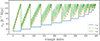 |
Fig. A.1. Triangle sides (rij) as a function of the triangle index, following the condition r12 ≤ r13 ≤ r23. |
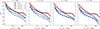 |
Fig. A.2. Cumulative S/N for the 2PCF and 3PCF measurements computed with the predicted Gaussian covariance according to Eqs. (A.1) and (A.2), as a function of the minimal scale included, rmin. |
Appendix B: 2PCF and 3PCF emulators
As detailed in Sect. 5, to efficiently sample the likelihood function as across the three cosmological parameters, we developed an emulator to obtain model predictions rapidly and accurately, in the first place, for the 3PCF, but also extending it to include the 2PCF. Indeed, the computational cost of the predictions for the coefficients ζℓ via Eq. (12) as well as the loop integrals coupled to the Hankel transform of Eq. (5) for the 2PCF makes it impractical to explore a broad range of cosmological parameters directly.
Neural network architecture of the emulator.
To address this issue, we constructed an emulator implemented in PyTorch4. The neural network, whose architecture is described in Table B.1, was trained using input samples drawn from a Latin hypercube sampling of the 3D, cosmological parameter space. This spans the ranges 109As ∈ [1.045, 3.135], h ∈ [0.63, 0.73], and ωcdm ∈ [0.09, 0.15]. The full models of both 2PCF and 3PCF can be written as sums of contributions each factorising the dependence on bias and nuisance parameters. This means that we can keep the analytical dependence on these parameters emulating the cosmology-dependence of each individual contribution. The emulator’s predictions were subsequently validated against a test set drawn from an independent sample to ensure their accuracy and reliability.
The metric chosen for assessing the emulator’s performance compares the systematic error Δξ on each separation bin for which r ≥ 7.5 h−1 Mpc for the 2PCF and Δζ on each triangular configuration for the 3PCF to their statistical error estimated from the covariance computed in Sect. 4 and with the binning choice adopted there. The statistical error is therefore relative to an observed volume of about 54 h−3 Gpc3, larger than any redshift bin expected for the Euclid spectroscopic sample (Euclid Collaboration: Blanchard et al. 2020). In particular, we required that the ratios Δξ/σξ and Δζ/σζ stayed, on average, below the 10% level. The distribution of this metric depends on both the separation (r) and the triangle configuration under consideration, the bias contributions, as well as on the sampled values of the cosmological parameters. This is illustrated by the normalised histograms shown in Fig. B.1. In this test, involving the full model predictions, we assumed a unitary linear bias b1 and c0, the bias relations presented in Eqs. (16) and (17), and the fitting function for b2(b1) obtained from numerical simulations in Lazeyras et al. (2016). All distributions, for both 2PCF and 3PCF at all four redshifts, are characterised by a median value for Δξ/σξ or Δζ/σζ well below 10%, decreasing slightly with redshift.
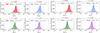 |
Fig. B.1. Normalised histogram of the ratio between the difference between emulated and exact modelling 2PCF predictions and the corresponding uncertainty, Δξ/σξ (top four panels). Different colours refer to different redshift snapshot, while the dashed black line represents the median of the distribution. The same quantity for the 3PCF, Δζ/σζ, is shown in the bottom four panels, for the different redshifts. |
This assessment ensures that the emulation process for both the 2PCF and the 3PCF is sufficiently accurate for the analysis presented in this work, but, in practice, also for a direct application to Euclid data or measurements from Stage IV surveys. We estimated a possible effect of systematic errors in the emulated prediction by adding in quadrature the mean value of Δξ and Δζ to the diagonal of the two covariance matrices finding no appreciable difference.
Finally, we notice that the emulator reduces the computational time required for the 3PCF evaluation from approximately 5 minutes per cosmological model to the order of 10−3 seconds.
Appendix C: Cosmological constraints
As a complement to the left panel of Fig. 6, in the in the top right, top left and bottom left panels of Fig. C.1 we present here the corresponding results at higher redshifts, namely z = 1.2, 1.5, and 1.8. We find that the same qualitative conclusions drawn at z = 0.9 continue to hold across redshift, with a general improvement in the precision of parameter inference at lower redshifts. A mild bias in the inferred values of As and b1 is observed, though still well within statistical compatibility with the expected values. We interpret this as a residual effect of projection, and note that all snapshots share the same seed. Moreover, we combined all redshift snapshots to derive constraints on the cosmological parameters As, ωcdm, h, as shown in bottom right panel Fig. C.1. In this combined analysis, we treated the cosmological parameters as shared across all redshifts while allowing the bias parameters to vary independently for each redshift bin, reflecting the expected evolution of galaxy bias with redshift. The combined constraints show significant improvement in precision compared to individual redshift analyses, demonstrating the enhanced constraining power achievable by combining multiple redshifts snapshots. We note that these snapshots are correlated as they share the same simulation seed, which should be taken into account when interpreting the statistical significance of the improvement.
Finally, in Fig C.2 we show the full extension of the right panel of Fig. 6, including all model parameters and, in particular, the non-linear galaxy bias terms, b2, b𝒢2, and bΓ3, and the EFT parameters, c0. This figure also illustrates how the impact of consistency relations on the bias parameter constraints becomes increasingly important as cosmological parameters are marginalised over, with the strongest effects visible for the degeneracy between As and b1. This highlights the critical role of consistency relations in enabling accurate cosmological inference once the cosmological parameter space is opened.
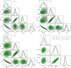 |
Fig. C.1. Top right, top left, and bottom left: Joint 2PCF+3PCF cosmological constraints and the linear bias b1 for individual redshift snapshots at z = 1.2, z = 1.5, and z = 1.8, following the format of Fig. 6. Bottom right: Combined cosmological constraints from all redshift bins (z = 0.9, 1.2, 1.5, and 1.8). |
All Tables
All Figures
|
Fig. 1. Top panels: 2PCF measurements for four comoving snapshots from the Flagship I simulation of the Model 3 HOD. Bottom panels: Same but for the 3PCF measurements. The triangular configurations are ordered by increasing values of r12, r13, and r23 under the condition r12 ≤ r13 ≤ r23, as depicted in Fig. A.1. The circles are colour-coded according to the η, while the vertical grey lines mark a group of triangles that share the same value of the smaller side (r12). |
| In the text | |
|
Fig. 2. GoF test for the bias 2PCF and 3PCF models with fixed cosmological parameters as a function of the minimal scale, |
| In the text | |
|
Fig. 3. Left panel: Marginalised 2D constraints at confidence intervals of 68.3% and 99.5%, on the nuisance parameters (bias and counter-term) from the 2PCF analysis (grey shaded areas) against the joint 2PCF and 3PCF analysis for several values of |
| In the text | |
|
Fig. 4. Marginalised constraints on the cosmological parameters and linear bias from a joint 2PCF and 3PCF analysis. The posterior mean along with its uncertainties is displayed as a function of the minimal scale ( |
| In the text | |
|
Fig. 5. Performance metrics for the full-shape, joint analysis of the 2PCF and the 3PCF. All quantities are shown as a function of the minimal scale ( |
| In the text | |
|
Fig. 6. Left panel: Marginalised 2D and 1D posterior distributions at z = 0.9 from the joint 2PCF and 3PCF analysis of the cosmological parameters h, ωcdm, and As and the linear bias parameter b1 for various 3PCF scale cuts ( |
| In the text | |
|
Fig. A.1. Triangle sides (rij) as a function of the triangle index, following the condition r12 ≤ r13 ≤ r23. |
| In the text | |
|
Fig. A.2. Cumulative S/N for the 2PCF and 3PCF measurements computed with the predicted Gaussian covariance according to Eqs. (A.1) and (A.2), as a function of the minimal scale included, rmin. |
| In the text | |
|
Fig. B.1. Normalised histogram of the ratio between the difference between emulated and exact modelling 2PCF predictions and the corresponding uncertainty, Δξ/σξ (top four panels). Different colours refer to different redshift snapshot, while the dashed black line represents the median of the distribution. The same quantity for the 3PCF, Δζ/σζ, is shown in the bottom four panels, for the different redshifts. |
| In the text | |
|
Fig. C.1. Top right, top left, and bottom left: Joint 2PCF+3PCF cosmological constraints and the linear bias b1 for individual redshift snapshots at z = 1.2, z = 1.5, and z = 1.8, following the format of Fig. 6. Bottom right: Combined cosmological constraints from all redshift bins (z = 0.9, 1.2, 1.5, and 1.8). |
| In the text | |
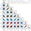 |
Fig. C.2. Same as the right panel of Fig. 6 but showing the full set of model parameters. |
| In the text | |
Current usage metrics show cumulative count of Article Views (full-text article views including HTML views, PDF and ePub downloads, according to the available data) and Abstracts Views on Vision4Press platform.
Data correspond to usage on the plateform after 2015. The current usage metrics is available 48-96 hours after online publication and is updated daily on week days.
Initial download of the metrics may take a while.