| Issue |
A&A
Volume 707, March 2026
|
|
|---|---|---|
| Article Number | A99 | |
| Number of page(s) | 21 | |
| Section | Cosmology (including clusters of galaxies) | |
| DOI | https://doi.org/10.1051/0004-6361/202556374 | |
| Published online | 27 February 2026 | |
A comparative test of different pressure profile models in clusters of galaxies using recent ACT data
Department of Physics, Xi’an Jiaotong–Liverpool University, Suzhou Dushu Lake Science and Education Innovation District, Suzhou Industrial Park 111 Ren’ai Road Suzhou 215123, People’s Republic of China
★ Corresponding author: This email address is being protected from spambots. You need JavaScript enabled to view it.
Received:
11
July
2025
Accepted:
13
January
2026
Abstract
Context. The electron pressure profile is a convenient tool to characterize the thermodynamic state of a galaxy cluster, with several studies adopting a “universal” functional form.
Aims. This study aims at using Sunyaev-Zel’dovich (SZ) data to test four different functional forms for the cluster pressure profile: generalized Navarro-Frenk-White (gNFW), β-model, polytropic, and exponential. The goal is to assess to what level they are universal over a population-level cluster sample.
Methods. A set of 3496 ACT–DR4 galaxy clusters, spanning the mass range [1014,1015.1] M⊙ and the redshift range [0, 2], is stacked on the ACT–DR6 Compton parameter y map over ∼13 000 deg2. An angular Compton profile is then extracted and modeled using the theoretical pressure recipes, whose free parameters are constrained against the measurement via a multistage Markov chain Monte Carlo approach. The analysis is repeated over cluster subsamples spanning narrower mass and redshift ranges.
Results. All functional forms are effective in reproducing the measured y profiles within their error bars, without a clearly favored model. While best-fit estimates are in broad agreement with previous findings, hints of residual subsample dependency are detected favoring higher amplitudes and steeper profiles in high-mass, low-redshift clusters.
Conclusions. Population-level cluster studies based on SZ data alone are likely unable to accurately constrain different pressure profile models. Residual trends at the population level as well as scatter at the individual cluster level undermine the universal pressure model assumption whenever high precision is required. Finally, functional forms that differ from the gNFW prove equally effective while being more physically motivated.
Key words: galaxies: clusters: general / galaxies: clusters: intracluster medium / large-scale structure of Universe
© The Authors 2026
 Open Access article, published by EDP Sciences, under the terms of the Creative Commons Attribution License (https://creativecommons.org/licenses/by/4.0), which permits unrestricted use, distribution, and reproduction in any medium, provided the original work is properly cited.
This article is published in open access under the Subscribe to Open model. This email address is being protected from spambots. You need JavaScript enabled to view it. to support open access publication.
1. Introduction
As the largest virialized structures in our Universe, clusters of galaxies encode a wealth of information about cosmology and astrophysics alike (Voit 2005; Allen et al. 2011). The task of linking cluster observational properties with theoretical models generally requires proper characterization of the intracluster medium (ICM), which contains the majority of a cluster’s baryonic mass (≲90%) in the form of a hot (107–108 K) and diffuse (10−4–10−2 cm−3) plasma composed primarily of ionized hydrogen and helium (Markevitch & Vikhlinin 2007).
The high temperature of the ICM has traditionally been exploited by observations in X-ray wavelengths (Sarazin 1988; Voges et al. 1999; Hicks et al. 2008; Mehrtens et al. 2012; Bulbul et al. 2024). In more recent years, cluster surveys in radio wavelengths have also gained relevance (Birkinshaw 1999; Carlstrom et al. 2002) by targeting the cosmic microwave background spectral distortion signature of the Sunyaev-Zel’dovich (SZ) effect (Sunyaev & Zeldovich 1972). The latter is proportional to the Compton parameter y, which quantifies the line-of-sight (LoS) integrated electron pressure. Sunyaev-Zel’dovich observations have been used not only to compile cluster catalogs of increasing size (Planck Collaboration XXVII 2016; Hilton et al. 2021; Kornoelje et al. 2025), but also to construct maps of the Compton parameter over extended regions of the sky (Planck Collaboration XXII 2016; Coulton et al. 2024).
From a theoretical point of view, it is customary to model the ICM as a spherically symmetric gas distribution, whose properties depend on the nominal radial separation from the cluster center. By combining the radial dependence of the ICM temperature and density, and considering that the ICM is ionized, the electron pressure profile is the most suitable physical quantity to characterize a cluster’s thermodynamic state. While real systems are expected to show deviations from this spherical symmetry, due to, for example, asphericities or local turbulence (Weinberger et al. 2017; Adam et al. 2025), radial profiles can still provide a mean baseline that is effective in reproducing integrated quantities such as the total cluster mass or the total X-ray/SZ fluxes. As such, they are fundamental ingredients in scaling relations between cluster masses and their observational proxies (Kravtsov et al. 2006; Vikhlinin et al. 2009; Planck Collaboration V 2013; Gallo et al. 2024). More crucially, if gravity dominates the cluster formation process, theory predicts the ICM to be approximately self-similar, implying that clusters of different masses and redshifts can be mapped onto each other through simple scaling relations for density, temperature, and pressure (Kaiser 1986; Arnaud et al. 2010). It is therefore interesting to test this self-similarity scenario and assess whether the same functional form for the radial pressure profile can be adopted to model the ICM in clusters with different masses and at different redshifts. This would imply the existence of a “universal” recipe, in which the electron pressure depends exclusively on a scaled separation from the cluster center, and in which the dependence on the cluster mass and redshift can be conveniently factorized out as a global scaling function.
Several studies in the literature have focused on a specific version of such a model, generally referred to as the “universal pressure profile” (UPP; Nagai et al. 2007; Arnaud et al. 2010) obtained as a generalization of the Navarro–Frenk–White (NFW) parameterization used to model dark matter profiles from simulations (Navarro et al. 1997). The aforementioned studies tested the UPP against cluster observations to constrain the parameters entering its functional form. Studies targeting reduced samples of high mass clusters (Nagai et al. 2007; Arnaud et al. 2010; Planck Collaboration V 2013; Pointecouteau et al. 2021; He et al. 2021) benefit from high-quality data of well-resolved systems. Their results, however, are somewhat limited in their range of applicability and are most likely affected by sample biases. More worryingly, the existing best-fit estimates for the UPP parameters show large scatter across different studies, hinting at the existence of strong degeneracies, which hamper a solid physical interpretation of individual parameter values. On the other end of the scale, large population studies (Gong et al. 2019; Tramonte et al. 2023) can provide results with a broader range of applicability. However, they are more affected by possible systematics in the dataset and by a loss of precision when the average profiles are applied to individual objects.
The study in Tramonte et al. (2023, hereafter T23) was the first to test the universal pressure profile model on a complete and representative sample of galaxy clusters. The sample merged the contributions of different existing cluster catalogs derived from optical observations, for a total of 23 820 objects spanning the mass range [1014,1015.1] M⊙ and the redshift range [0.02, 0.98]. The study measured the averaged cluster Compton parameter profile by stacking these clusters on the Compton parameter maps based on Planck (Planck Collaboration XXII 2016) and Atacama Cosmology Telescope (ACT, Madhavacheril et al. 2020) data. The UPP was then tested by comparing its predicted y profiles with the measurements. The study also considered cluster subsamples to explore possible evolutions of the model with different cluster mass and redshift regimes. Overall, the fitted profile model was effective in reproducing the SZ measurements in all cases, with the best-fit parameter values being broadly consistent with previous results in the literature. Although individual parameter values were found to depend on the chosen cluster subsample, the study did not provide any compelling evidence for a residual dependence on the cluster mass and redshift.
The present study is a new attempt at testing theoretical models for the ICM on Compton parameter profiles extracted from cluster stacks on y-maps, considering a population-level sample (∼103 clusters) and recent ACT data. While the methodology is similar to the one followed in T23, there are some important differences. First, the ACT y-map adopted in this study is considerably larger than the one used in T23, by a factor of ∼6 in the footprint area. Second, this study considers a homogeneous cluster catalog constructed via a blind search on the same SZ data employed for the y map. The cluster sample used in T23, on the contrary, was a heterogeneous combination of different catalogs built from optical data and as such suffered from possible systematic effects in the mass definition1. Finally, the scope of this work is broader, as it considers not only UPP parameterization but also different recipes for modeling the electron pressure distribution in the ICM. Again, the goal is first to test whether these models can be effective in reproducing observed features in the cluster SZ emission and subsequently to assess possible residual dependencies of the model parameters on cluster mass and redshift (as deviations from universality).
This paper is organized as follows. Sec. 2 describes the dataset used in this study. The y-profile measurement procedure and results are presented in Sec. 3, while the theoretical modeling is detailed in Sec. 4. Sec. 5 explains the parameter estimation approach and results, while Sec. 6 discusses the findings. Finally, conclusions are drawn in Sec. 7. The present study adopts a spatially flat Lambda cold dark matter cosmological model with fiducial parameter values h = 0.674, Ωm = 0.315, Ωb = 0.0493, σ8 = 0.811, and ns = 0.965 (Planck Collaboration VI 2020).
2. Data
The Compton parameter map and cluster catalog considered in the present analysis are described in the following subsections. Figure 1 provides a visual representation of the combined dataset.
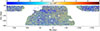 |
Fig. 1. Visual representation of the dataset employed in this study. The ACT DR6 Compton parameter map is plotted on an equirectangular projection – the white region highlighting the mask footprint. The blue spots show the positions of the 4195 clusters from the ACT DR5 catalog. |
2.1. Compton parameter map
This study employs the Compton parameter map described in Coulton et al. (2024), which is publicly available at the NASA Legacy Archive for Microwave Background Data (LAMBDA) page for AdvACT products2. The map was generated via a blind component separation pipeline – an adapted version of the internal linear combination (ILC) method in wavelet frame – applied to individual frequency maps from Planck NPIPE, ACT DR4, and DR6 (the two experiments being complementary in terms of spatial resolution). The final footprint was constrained by the ACT observing area to approximately one third of the sky, or ∼13 000 deg2, and the final map resolution is 1.6 arcmin. The map was delivered in a flat plate carrée (equirectangular) projection on a 2D frame, with axes parallel to the right ascension (RA) and declination (Dec) directions, and pixel uniform size of 0.5′ in both RA and Dec. The present study also makes use of the associated sky mask, also provided as part of the data release, which combines the Planck Galactic plane mask covering 30% of the sky, an ACT footprint mask, and a mask of the bright extended sources in the individual frequency maps.
As discussed in Coulton et al. (2024), cosmic infrared background (CIB) residuals in the Compton map can be a potential source of contamination. Such residuals can be modeled as modified blackbodies in their frequency spectral energy distribution (SED), and subtracted. The result is a set of CIB de-projected Compton parameter maps, also available as part of the data release, which differ on the adopted values of the parameters entering the CIB SED functional form. The reference also warns, however, that existing uncertainty on the actual CIB SED can result in incomplete removal of this contaminant from the final map. Moreover, further de-projections come at the price of possibly removing a part of the target tSZ signal. For these reasons, the standard y-map (without any CIB de-projection) was adopted as the fiducial map in the present study. The impact of possible CIB residuals on the results of this study is discussed in Appendix A, where it is shown that, at the reconstructed profile level, using de-projected versions of the map yields differences within the overall uncertainties.
2.2. Cluster catalog
This study employs the galaxy cluster catalog described in Hilton et al. (2021), which is publicly available at the NASA LAMBDA page for ACTPol products3. Cluster candidates were identified via a blind search on ACT DR5 co-added 98 and 150 GHz maps using a multifrequency matched filter. Masking of bright point sources and of regions with high dust emission (galactic latitudes |b|< 20° plus others identified on Planck 353 GHz map), high-flux on the ACT 150 GHz maps, or deemed unfit after visual inspection, resulted in an effective search area of 13 211 deg2. The search yielded 8878 cluster candidates detected with signal-to-noise ratio (S/N) > 4; of these, 4195 objects were confirmed as clusters after cross-matching with optical/IR surveys, which also provided redshift estimates for the detections. Spectroscopic redshift estimates are available for 1648 (∼39.3%) objects, the remaining ∼60.7% only quoting photometric redshift estimates.
Cluster masses were estimated using the scaling relation from Arnaud et al. (2010) to convert the SZ signal to mass. Estimates are quoted as spherical overdensity masses M500, i.e., enclosing a region whose mean density is equal to 500 times the critical density of the Universe at that redshift. As the aforementioned scaling assumes hydrostatic equilibrium in the ICM, the resulting masses are known to underestimate the true cluster masses (see, e.g., Miyatake et al. 2019, and reference therein). The catalog also provides bias-corrected mass estimates obtained using a common richness-based weak-lensing (WL) mass calibration factor, which shows that SZ-estimated masses underestimate WL-estimated ones by ∼30%. The cluster mass values M500 adopted in this study, however, are those quoted in the catalog as obtained directly from the SZ measurements, without correcting for the bias derived from the assumptions of hydrostatic equilibrium.
As the optical/IR confirmation results in very high purity (the probability for a detection to be an actual cluster), the selection function of this catalog is determined by its completeness (the probability of a real cluster to be detected). The latter was evaluated to be larger than 90% for masses M500 > 3.8 × 10¹⁴ M⊙ at redshift z = 0.5 (the median redshift of the sample). While this average value was found to have a very mild redshift dependence, the completeness evaluated in different regions of the cluster search areas showed high levels of inhomogeneity, which is a result of ACT observational scanning strategy. In the present study, the selection function is naturally accounted for in the theoretical modeling, as explained in Sec. 4.1.
Before concluding this section, it is relevant to acknowledge the impact of Eddington bias on the catalog employed in this study and hence on the cluster signals measured in Sec. 3. As the catalog was generated via a blind search on the same dataset employed to generate the y-map, noise fluctuations in the map potentially overestimate the y signal of the cataloged clusters. The effect is especially relevant for low-mass systems, which if located on top of a positive noise fluctuation can still enter the catalog even though their true SZ signal is slightly below the detection threshold. A complete selection function to correct for this effect would need to factor in the effects of map noise, filtering, detection pipeline, and intrinsic scatter in the SZ flux to the mass scaling relation, detection thresholds, and survey inhomogeneity. Such a selection is not available, particularly not as an explicit function of cluster mass and redshift. While the uncorrected Eddington bias does overestimate the amplitude of the reconstructed profiles, it also biases high the cataloged cluster mass values adopted to model the profiles theoretically in Sec. 4.1. As stated, these masses are indeed those obtained directly from the SZ measurement, uncorrected for any bias or selection effect. In other words, the amplitude overestimation equally affects the measured and the modeled y profiles. The resulting best-fit parameter values are then reasonably robust despite the bias. Furthermore, the conclusions from this study mostly focus on the comparison and viability of different theoretical models for the cluster pressure profile, rather than on the search for an ultimate universal set of parameter values.
3. Measurements
As anticipated in Sec. 1, cluster Compton parameter profiles are the primary observable considered in this study for testing ICM theoretical models. This section describes the methodology adopted to reconstruct such profiles and assesses the results.
3.1. Cluster samples
As visible from Fig. 1, some clusters from the ACT DR5 catalog lie outside the map footprint. The catalog was queried to select only the clusters that do not overlap with the mask described in Sec. 2.1, resulting in a total of 3946 objects. This catalog was split into smaller samples spanning different mass and redshift ranges. This analysis considers three mass bins bound by edge points [14.0, 14.3, 14.6, 15.1] (in units log10(M500/M⊙), with bias-uncorrected catalog masses M500) and three redshift bins, bound by edge points [0.0, 0.4, 0.8, 2.0]. The catalog was then binned in both mass and redshift over this grid, resulting in nine nonoverlapping samples (one for each combination of a mass bin and a redshift bin); six marginalized cases (the full mass span of the catalog for each redshift bin and the full redshift span of the catalog for each mass bin); and the complete unmasked catalog, for a total of 16 different samples.
Fig. 2 shows the catalog distributions in mass and redshift, highlighting the edges of the chosen bins. Due to the highly nonuniform trends of these distributions, each (M, z) bin has a substantially different number of clusters. The right panel in Fig. 2 also shows some degree of correlation between the two quantities. The most massive clusters are generally found at the lowest redshifts, as expected from a bottom-up scenario for structure formation. It is also possible to notice a slight rightward shift in the point distribution for higher redshifts, which is likely evidence of Malmquist bias affecting the cluster catalog. Again, these features were properly accounted for as selection effects in the theoretical modeling (Sec. 4.1).
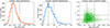 |
Fig. 2. Left and middle panels: distribution in mass and redshift of the full cluster sample adopted in this study. Right: catalog scatter across these two quantities. In all panels, the dashed lines mark the edges of the chosen bins in the corresponding quantity. |
3.2. Stacks
Each of the 16 samples was stacked on the ACT map to obtain a measurement of the integrated cluster emission. The stacking procedure is ultimately a weighted average that employs the Compton parameter map as the “signal” map and the mask as the “weight” map with pixels valued 0 or 14. For the generic i-th cluster, a square region centered on its nominal position was extracted from both the y map and the weight map, resulting in two sub-maps Yi and Wi, respectively. The final, stacked map was obtained as
 (1)
(1)
where N is the number of clusters in the considered sample and W is the total weight of the stack.
Because the ACT Compton parameter map was delivered in an equirectangular projection with a uniform pixelization in both coordinate axes, pixels located farther from the celestial equator subtend a smaller solid angle on the sky. More precisely, a pixel with generic declination δ spans an effective RA range shorter by a factor cos δ compared to a pixel on the equator (δ = 0). As the y map extends down to latitudes of ∼ − 60°, this implies that pixels at the lower edge of the map would actually subtend a solid angle which is about half of their nominal size. If not corrected for, this effect would produce spurious elongations along the RA direction of any features within the final stacks; such ellipticities would in turn result in an artificial stretching of the associated angular profiles.
This effect was corrected for at the level of the individual cluster sub-maps Yi and Wi, prior to the stack sums in Eq. (1). In those sub-maps, the RA separation of each pixel from the cluster is multiplied by the cosine of the cluster declination. The sub-maps were then projected onto a common frame consisting of a square map centered on the cluster nominal coordinates, with size 30′×30′ and 320 pixels in each axis. The extension of this frame was chosen to ensure the final stacks are able to capture all features of the cluster emission, down to its outskirts. The resolution was chosen to be high enough to retain information from the resolution of the parent ACT Compton map. Clearly, the shape of the region initially trimmed out of the ACT map was not a square but a rectangle, whose RA side was 30′/cos δc where δc is the declination of the considered cluster. This ensured that, after the declination correction, the rectangle would fit exactly into the reference stack frame.
This approach is an important upgrade compared to the stacking procedure adopted in T23, where all pixels were assumed to have equal area and individual cluster regions were simply trimmed out of the map and stacked. That study, however, employed the ACT-DR4 y maps, which did not extend more than ∼19° away from the equator. This results in declination correction factors always below ∼5%, justifying the approximation adopted in that work.
A summary table of the stacks obtained for all the 16 cluster samples is shown in Fig. 3. To better show the features in the averaged cluster signal, each color scale was saturated to the extreme values in the corresponding map, and the plot area focuses on a smaller 12′×12′ around the center. In all cases, the cluster emission is clearly detected with a high contrast against the background. We can notice that the contrast is the highest for the top mass bin, which yields the highest peak amplitude. We can also notice that higher redshift stacks appear smaller in angular size, an effect due to the increase in the angular diameter distance within the probed redshift range. Although some irregularities affect the signal contours, the declination correction performed during the stack results in overall round profiles with no clear evidence of residual ellipticities.
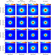 |
Fig. 3. Summary plot showing the stacks on the ACT y-map of all the 16 cluster samples, described in Sec. 3.1, with labels clarifying the associated mass and redshift intervals. Although the final stack maps are 30′×30′ in size, this figure zooms in on the central 12′×12′ square to better show the details in the cluster signal. |
3.3. Profiles
A circularly symmetrized angular Compton parameter profile y(θ) was extracted from each of the 16 stacks. Pixels in each stack map were assigned to bins in the radial separation from the center, and the average of all the pixels within the i-th ring was taken as the value of the Compton profile at the corresponding mean angular separation, y(θi). The size of each angular separation bin was set to 0.5′, which is the same as the resolution of the original ACT Compton parameter map.
As we are interested in the y amplitude with respect to the mean map background level, from each of the 16 profiles a zero-level profile was subtracted, determined as follows. For each of the 16 samples, the associated stack was repeated 500 times (following the same procedure described in Sec. 3.2), but this time shuffling the coordinates of the clusters within the allowed Compton map footprint. This results in 500 randomized-amplitude profiles, whose average was taken as the zero-level profile subtracted from the real cluster profiles. Fig. 4 shows the result of this approach. For each sample, individual lines represent the profiles extracted from each randomized stack. The thicker central line shows their average, and the dotted lines show the 1-sigma confidence interval. The figure shows that all average profiles are well compatible with zero. As expected, we observe larger scatter in the samples containing a lower number of clusters, an effect particularly evident in the largest mass bin. Although the average profiles are not exactly zero and as such are to be subtracted from the real cluster profiles, their mean value is negligible compared to the peak amplitude of the profiles extracted from the stacks. In summary, this test shows no relevant zero-level systematics affecting our stacks.
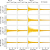 |
Fig. 4. Estimation of the mean background level in the stacks. For each mass and redshift bin, the colored bundle represents the set of all 500 profiles extracted from the shuffled stacks. The solid darker line shows their average, taken as the zero-level profile, and the dashed black lines show the 68% confidence interval around the mean. |
Uncertainties on the measured profiles and correlation values between different angular bins were evaluated via covariance matrices. For each cluster sample, another set of 500 randomized stacks was produced. This time each new cluster sample was generated via a bootstrap approach by randomly selecting the same number of clusters from the corresponding original (M, z) sample allowing repetition. The covariance matrix Cov(θi, θj) between the two angular bins θi and θj was then obtained as
![Mathematical equation: $$ \begin{aligned} C(\theta _i,\theta _j) = \dfrac{1}{N_{\rm rand}} \sum _{k = 1}^{N_{\rm rand}} [{ y}_k(\theta _i)-\bar{{ y}}(\theta _i)] [{ y}_k(\theta _j)-\bar{{ y}}(\theta _j)], \end{aligned} $$](/articles/aa/full_html/2026/03/aa56374-25/aa56374-25-eq2.gif) (2)
(2)
where Nrand = 500 is the number of random realizations, the index k identifies the individual random stack, and  is the average value of the profile at the angular bin θi, across all random realizations:
 (3)
(3)
The correlation matrix Corr(θi, θj) can be computed normalizing the covariance matrix as in
 (4)
(4)
The correlation matrices for all 16 stacks are shown in Fig. 5 and are a measurement of the level of statistical independence between bin pairs. The figure shows that residual correlations persist even for largely separated bins, with the effect being more pronounced for the lowest-redshift samples yielding the broader profiles.
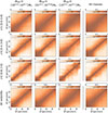 |
Fig. 5. Correlation matrices associated with the reconstructed Compton parameter profiles over the relevant angular span, for all mass and redshift bins. |
The profiles for all 16 stacks are shown in Fig. 6, grouping different redshift bins for each individual mass bin. These profiles are zero-level subtracted and show the 1-sigma uncertainty as a shaded region. The latter was estimated, for each bin θi, as the square root of the corresponding diagonal entry in the covariance matrix,  . Exclusively for visualization purposes, these profiles (and their uncertainties) were evaluated with a finer angular resolution, with a bin size of 0.1′ (the same consideration holds for the background estimation profiles in Fig. 4). Notice that, while the stack maps extend to angular separations of ∼15′ from the center, these plots show the profiles only up to 11′, as in all cases this separation is enough to make the Compton parameter amplitude compatible with the zero level. This upper limit of 11′ was maintained also in the modeling part of the present study. All panels in Fig. 6 also include the ACT beam, whose angular profile was computed assuming a perfectly Gaussian shape with full width at half maximum (FWHM) equal to 1.6′, showing that all Compton profiles are resolved with the resolution of the ACT y-map.
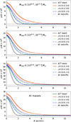 |
Fig. 6. Circularly symmetrized Compton parameter angular profiles extracted from the 16 stacks shown in Fig. 3, background subtracted, and showing the 1-sigma uncertainty per bin as a shaded region. Profiles are grouped according to their mass bin, showing different redshift bins in each panel. The ACT beam profile is included for comparison. |
To conclude this section, following the standard approach for correlated data, the significance of the measurement of each profile can be quantified via a chi-square as in
 (5)
(5)
where Nb = 22 is the total number of bins considered over the angular range from 0 to 11′, and I is the inverse covariance matrix corrected by the Hartlap factor (Hartlap et al. 2007)
 (6)
(6)
(Nrand = 500 is the number of random realizations used to estimate the covariance matrices). In this expression, y(θi) is to be regarded as the difference between the measurement and the null hypothesis (i.e., no signal, y = 0). Higher χ2 values were therefore obtained for profiles that deviate more from zero and were thus detected with higher significance (the same approach was adopted in T23). Because the value of the χ2 from Eq. (5) scales with Nb, an effective significance per angular bin was calculated as χb2 = χ2/Nb. Values of χb2 > 1 indicate that, on average, the measured profile deviates from zero (the null hypothesis) more than expected from the noise. The per-bin significance values are quoted in Table 1 for all 16 samples. The table shows that the profiles were reconstructed with a very high significance of 10–20 in all cases.
Statistics of the cluster samples employed in this study.
4. Model
The following subsections detail the theoretical modeling of the measurements presented in Sec. 3. The approach adopted to model the joint contribution of different clusters to the measured y-profiles is presented in Sec. 4.1. The specific theoretical recipes for the ICM pressure profiles, instead, are detailed in Sec. 4.2.
4.1. The Compton parameter profile for a cluster sample
Each Compton profile y(θ) reconstructed in Sec. 3.3 merges the contributions of clusters of different masses and redshifts. In principle, if the Compton parameter profile yi(θ) generated by the i-th cluster is known, the mean profile obtained with the stack of a given cluster sample can be predicted as
 (7)
(7)
where Ncl is the number of clusters in the sample. To be comparable to the measured profiles, the smoothing effect introduced by ACT beam should be accounted for. In real space, this is implemented mathematically via a convolution between the emission profile y(θ) and the beam profile B(θ):
 (8)
(8)
We can reasonably assume the beam profile to be a perfect Gaussian (normalized to unit integral) as in
![Mathematical equation: $$ \begin{aligned} B(\theta ) = \frac{1}{\sigma \sqrt{2\pi }}\exp {\left[-\frac{\theta ^2}{2\sigma ^2}\right]}, \end{aligned} $$](/articles/aa/full_html/2026/03/aa56374-25/aa56374-25-eq11.gif) (9)
(9)
where  and FWHM = 1.6’ for ACT. As the stack weight maps W are practically uniform in all stack cases (with central amplitude differences ≲1%) Eqs. (7) and (8) represent the mathematical equivalent of the stacking process, but for the theoretical profiles. Strictly speaking, the stack is the average of the individual cluster profiles already convolved with the beam; however, since both stack and beam smoothing are linear operations, convolving the average profile is the same as averaging the convolved profiles.
Despite its apparent simplicity, this approach for predicting the measured profiles is computationally demanding and not suitable for the statistical inference study presented in Sec. 5. Indeed, for each cluster sample, this would require the computation of ∼102–103y-profiles (depending on the chosen mass-redshift bin) for each step of the parameter estimation code, which requires about ∼105 iterations to converge (Sec. 5).
A more general and efficient approach to perform the average is to consider the generic profile y(θ; M500, z) of a cluster of mass M500 at redshift z, and integrate it over mass and redshift as in
 (10)
(10)
where d2V/dzdΩ(z) is the comoving volume element, dn/dM500(M500, z) is the halo mass function, and S(M500, z) is a selection function quantifying any deviation of the sample cluster abundance from the theoretical mass function. The normalization factor ncl is the total number density (per unit solid angle) of clusters within the sample mass span [Mlow, Mtop] and redshift span [zlow, ztop]:
 (11)
(11)
In other words, the mean Compton profile of a cluster sample is the weighted average of the quantity y(θ; M500, z) over the sample mass and redshift spans, with the weighting function being the product of the comoving volume element, the mass function, and the selection function. While the comoving volume element is uniquely defined for a given cosmology and widely used parameterizations for the halo mass function exist in the literature, the selection function is a quite challenging component to quantify. An effective selection modeling should include a number of effects such as instrumental sensitivity and observational strategy, performance of the cluster finding algorithm, and subsequent catalog cuts. Furthermore, the result should be expressed in terms of a suitable function of mass and redshift. This task is impractical, especially considering the importance of a proper characterization of the function S(M, z) to not bias the model testing.
A way to circumvent this issue, introduced in Gong et al. (2019) and also adopted in T23, is to split both the mass and redshift spans into a suitable set of smaller intervals, and approximating the Compton parameter profiles of all clusters within a given interval with the one of a hypothetical cluster whose mass and redshift are equal to the interval midpoints. This way, Eqs. (10) and (11) become
 (12)
(12)
where NM and Nz are respectively the number of mass and redshift intervals,  and
and  are the midpoints of the i-th mass and j-th redshift intervals, and Nij is the number of clusters in the corresponding cross mass-redshift interval (the quantity Ncl is again the number of clusters in each of the stacked samples). Thanks to the weighting Nij factors, the average estimate of the Compton parameter profile via Eq. (12) naturally encodes the selection associated with each sample.
Clearly, Eq. (12) introduces an approximation in the theoretical prediction, which improves with larger values for NM and Nz. A compromise must be made with computational efficiency, which rather favors lower values for NM and Nz. Given, for instance, a cluster sample with a fixed number of mass and redshift intervals, the accuracy in the estimation of the average profile depends on how many clusters there are in the sample and how their M500 and z values differ from the selected interval midpoints. It is then reasonable to expect that the interval numbers NM and Nz depend on the considered cluster sample. This study adopts NM = 4, NM = 3, and NM = 7 for the lowest, intermediate, and highest mass bin, respectively, and Nz = 6, Nz = 3, and Nz = 4 for the lowest, intermediate, and highest redshift bin, respectively. The marginalized bins use the union of all the intervals from individual bins, so NM = 14 and Nz = 13 (now intervals have different sizes). These values were chosen to yield averaged profiles whose difference from the full computation in Eq. (7) is well below the uncertainties in the measured y-profiles, over the full range of θ.
This approach simplifies the theoretical prediction for a chosen cluster sample into the task of computing NM × Nz Compton parameter profiles, i.e., ∼10 − 100 (depending on the chosen cluster sample) in order of magnitude, which is considerably faster compared to the ∼103 profiles in the most populated bins. This allows us to incorporate the prediction into a suitable parameter estimation code. Moreover, because Eq. (12) uses the number of clusters within each interval instead of individual cluster masses, this strategy is also somewhat less sensitive to possible uncertainties affecting the mass estimates (as long as those uncertainties are smaller than the chosen interval size).
4.2. The Compton parameter profile for individual clusters
We are now left with the problem of computing the Compton parameter profile y(θ; M500, z) for chosen values of the cluster mass M500 and redshift z. As anticipated in Sec. 1, the Compton parameter can be obtained via the LoS integral of the electron pressure Pe. More precisely, for a cluster of mass M500 at redshift z, the Compton parameter value at a separation θ from the center can be computed as
 (13)
(13)
In the equation above, ℓ is the LoS distance variable, DA(z) is the angular diameter distance to the redshift z of the cluster, and the LoS integration extends out to
 (14)
(14)
where Rcl is the radius of the cluster. It is customary to set Rcl = 5 R500, where the overdensity radius can be computed from the cataloged masses5M500 as
![Mathematical equation: $$ \begin{aligned} R_{500} = \left[ \frac{3M_{500}}{4\pi \cdot 500\,\rho _{\rm c}(z)} \right]^{1/3}, \end{aligned} $$](/articles/aa/full_html/2026/03/aa56374-25/aa56374-25-eq20.gif) (15)
(15)
with ρc(z) being the critical density of the Universe at redshift z. It is possible to verify that extending the range of integration in Eq. (13) using values of Rcl higher than 5 R500 adds only a negligible contribution to the integral.
The problem now has narrowed to the choice of a suitable functional form for the electron pressure profile Pe(r; M500, z), with r being the radial separation from the cluster center. If we assume that different clusters share the same functional form for the profile shape, it should be possible to factorize out the dependence on r as in
 (16)
(16)
The function ℙ(x) is supposed to reproduce the profile shape for clusters of any mass and redshift. Clearly, in order to account for the different ICM spatial extension in clusters of different mass, ℙ should be a function of a scaled radial separation x = r/rs, with rs being a suitable scale radius. The latter can be defined as
 (17)
(17)
where c500 is a universal concentration parameter quantifying the deviation of the scale radius rs from the overdensity radius R500, with lower values of c500 resulting in broader profiles. As Eq. (17) clearly shows, c500 is initially taken to be independent of mass and redshift. This assumption is put to a test in Sec. 5.
The first factor in Eq. (16) is an overall amplitude independent of the separation from the cluster center, which depends on the cluster mass and redshift. A convenient choice for this factor is a generalization of the characteristic cluster pressure P500 in the self-similar model:
![Mathematical equation: $$ \begin{aligned} \xi (M_{500},z) = \xi _0\, h^2 \,E^{8/3}(z)\left[\frac{M_{500}}{2.1h\times 10^{14}\,\mathrm{M}_{\odot }}\right]^{2/3+\alpha }, \end{aligned} $$](/articles/aa/full_html/2026/03/aa56374-25/aa56374-25-eq23.gif) (18)
(18)
where ξ0 = 3.367 × 10⁻³ keV cm−3, E(z) = H(z)/H0 encodes the redshift evolution of the Hubble parameter, and h = H0/100 km s−1 Mpc−1 is the dimensionless Hubble constant. For the case α = 0, the expression above represents the characteristic pressure P500, which quantifies the pressure at radius R500 required to prevent the gravitational collapse of a cluster of mass M500 at redshift z. The study conducted in Arnaud et al. (2010) showed that to remove residual mass dependencies in the universal pressure model, an extra contribution α = 0.12 should be added to the mass exponent of M500. This study includes the same additional scaling, as in principle the function ξ(M500, z) should include all the mass and redshift dependence. Again, this hypothesis is tested in Sec. 5. Notice that, as the scaled profile ℙ(x) also contains an adjustable amplitude factor, the actual absolute value of the function ξ(M500, z) is not crucial. What is important, however, is the functional dependence on mass and redshift shown in Eq. (18).
The core of the present study is actually to test different parameterizations for the scaled profile ℙ(x) by comparing the predicted mean y-profile against those extracted from ACT data. Based on its definition, it is already clear that ℙ(x) depends at least on two parameters: an overall amplitude and a concentration c500 used to define the scale radius. Any additional parameters entering the computation of ℙ(x) depend on its functional form, for which the present analysis considers the following four cases.
4.2.1. The universal pressure profile
The UPP6 reads
![Mathematical equation: $$ \begin{aligned} \mathbb{P} (x) = \frac{P_0}{x^{\gamma }\left[1+x^{\alpha }\right]^{(\beta -\gamma )/\alpha }}, \end{aligned} $$](/articles/aa/full_html/2026/03/aa56374-25/aa56374-25-eq24.gif) (19)
(19)
where apart from the overall normalization P0, the parameters γ, α, and β quantify the profile slopes at small (x ≪ 1), intermediate (x ≃ 1), and large (x ≫ 1) separations from the cluster center.
This generalized NFW (gNFW) functional form was first proposed in Nagai et al. (2007) to fit cluster pressure profiles reconstructed merging simulation results with Chandra-based X-ray data. The UPP was later the subject of a number of different studies aimed at testing its validity range or providing novel estimates on its parameters (see, e.g., Arnaud et al. 2010; Planck Collaboration V 2013; Sayers et al. 2016; Gong et al. 2019; Ma et al. 2021; He et al. 2021; Pointecouteau et al. 2021; Gallo et al. 2024, and references therein). The UPP was also the base model adopted in T23, where its parameter values showed no detectable residual dependencies on M500 or z within the error bars.
Despite proving effective in reproducing observed X-ray and SZ cluster emissions, the UPP functional form presents a few drawbacks, such as its unphysical divergence at x = 0, or the strong degeneracies existing between the different slope parameters. As a result of this last feature, the best-fit parameter values quoted in the aforementioned studies exhibit strong scatter (see for instance Table 1 in T23). In other words, while the combined effect of all parameter values in Eq. (19) provides a consistent prediction, the value assigned to each parameter individually alone cannot be trusted, thus preventing (to some extent) a proper physical characterization of the ICM pressure distribution.
In the present study, the free parameters considered for this functional form are P0, α and β. As is customary in other studies to test the UPP against SZ observables, the parameter γ was fixed to a nominal value of 0.31.
4.2.2. The β-model profile
Under the assumption of hydrostatic equilibrium and isothermality in the ICM, the electron number density profile can be conveniently fit using the functional form
![Mathematical equation: $$ \begin{aligned} n_{\rm e} = n_{\rm e0}\left[1+\left(\frac{r}{r_{\rm c}}\right)^2 \right]^{-\frac{3}{2}\beta }, \end{aligned} $$](/articles/aa/full_html/2026/03/aa56374-25/aa56374-25-eq25.gif) (20)
(20)
which is known as the isothermal β-model (Cavaliere & Fusco-Femiano 1976, 1978). Here, rc is a suitable core radius, ne0 is the central density, and the slope parameter β has typical values of ∼0.7. This is a well established model for cluster density profiles and has long been used to fit X-ray surface brightness in clusters (Birkinshaw 1999; Sarazin 1988). The theoretical motivations for this model and its evident simplicity come at the price of some inaccuracies when fitting extended datasets (Arnaud 2009). The recent study in Braspenning et al. (2025) proposes a more effective, modified version of this profile. This too comes at the price of a substantial increase in complexity and a set of seven free parameters.
This work adopts a simpler approach based on the original profile in Eq. (20). Under the assumption of isothermality, the electron pressure profile follows the same functional form as the density profile. It is then reasonable to propose the following functional form for the scaled cluster pressure profile:
![Mathematical equation: $$ \begin{aligned} \mathbb{P} (x) = P_0 \left[1+x^2 \right]^{-\frac{3}{2}\beta }, \end{aligned} $$](/articles/aa/full_html/2026/03/aa56374-25/aa56374-25-eq26.gif) (21)
(21)
where the normalization P0 and the slope β are free parameters. To some extent, this profile choice relaxes the assumption of isothermality, as the free slope β can accommodate possible variations in the temperature; nonetheless, temperature is still assumed to share the same scale radius rs as the density and to follow a similar decreasing trend for increasing separations from the center. Hereafter this profile is referred to as the β-model profile (BMP).
4.2.3. The polytropic profile
The polytropic assumption implies a simple power-law relation between a gas pressure P and density ρ in the form P ∝ ρΓ, where Γ is known as the polytropic index. Similarly to the case of the β-model approach, the polytropic one also assumes hydrostatic equilibrium; however, it is less restrictive as it does not require isothermality. This assumption was explored in the work by Bulbul et al. (2010) in combination with a NFW profile for the density distribution generalized by a parameter β, which quantifies the steepness of the gravitational potential. This results in a β-dependent functional form for the pressure profile, which in the limit β → 2 (corresponding to a standard NFW density profile) reads
![Mathematical equation: $$ \begin{aligned} \mathbb{P} (x) = P_0\left[\frac{1}{x}\ln (1+x) \right]^{n+1}, \end{aligned} $$](/articles/aa/full_html/2026/03/aa56374-25/aa56374-25-eq27.gif) (22)
(22)
where the exponent term n is related to the polytropic index via n = 1/(Γ − 1). Notice that in the equation above the singularity at x = 0 is only apparent because for x → 0 the function has limit P0. Hereafter the functional form in Eq. (22) is referred to as the polytropic profile (PTP). Although fixing β may result in a partial loss of applicability (particularly near cluster cores), the present study uses Eq. (22) as an additional model for the cluster pressure profile, again with the goal of using fewer parameters to mitigate their degeneracy. The free parameters considered for this functional form are P0 and n.
4.2.4. The exponential universal profile
This study also considers a new ansatz to model the scaled profile in the form
 (23)
(23)
which for clear reasons is labeled the “exponential universal profile” (EUP). While it is not justified by any simulation-based or analytical result, this profile is intended to be a simplified extension of the UPP. In this framework, the exponential factor e−γx replaces the UPP power factor x−γ, thus solving the central divergence. The function (1 + x)−ζ mimics the UPP bracket factor but with a simplified form, which can help remove the tight degeneracy between the UPP exponents α and β. In the present study, the free parameters considered for this functional form are P0, γ and ζ.
5. Model testing
This section is dedicated to a direct comparison between the angular Compton parameter profiles measured from the ACT y-map in Sec. 3, and those predicted using the theoretical recipe described in Sec. 4, using each of the universal models listed in Sec. 4.2. The goal is first to infer best-fit estimates on the model parameters to match the measurements, and second to assess which of the models can best reproduce the profile features reconstructed from observations. The results can also reveal parameter best-fit values drifts (if any) with mass and redshift, as this comparison was conducted for all of the 16 cluster samples considered in this study.
5.1. Parameter estimation method
For each profile model, its free parameters plus the concentration c500 were estimated with a Markov chain Monte Carlo (MCMC) approach implemented via the Python package emcee7, based on the affine invariant sampler from Goodman & Weare (2010). This method enables us to extensively sample the parameter space and reconstruct the posterior distributions on individual and pairs of parameters, thus allowing us to infer their best-fit values.
The MCMC runs are based on the following chi-squared definition:
![Mathematical equation: $$ \begin{aligned} \chi ^2(\Theta ) = \sum _{i = 1}^{N_{\rm b}}\sum _{j = 1}^{N_{\rm b}} \left[{ y}_i(\Theta )-{ y}_i^\mathrm{(m)}\right]\,C^{-1}_{ij}\,\left[{ y}_j(\Theta )-{ y}_j^\mathrm{(m)}\right], \end{aligned} $$](/articles/aa/full_html/2026/03/aa56374-25/aa56374-25-eq29.gif) (24)
(24)
where Nb is the number of angular bins, the indices i and j select a specific bin, y(Θ) is the Compton profile predicted using the parameter set Θ (and the corresponding theoretical model), y(m) is the measured Compton profile for the chosen cluster sample, and C−1 is the inverse of the covariance matrix for the same cluster sample (Sec. 3.3).
For each parameter, a flat prior probability distribution was adopted, within reasonable ranges justified by previous results in the literature. The procedure was repeated for each profile model and each cluster sample, yielding 64 MCMC runs consisting of 12 walkers and 500 000 steps, enough to ensure convergence. Chains were then trimmed to remove the first 10% (assumed to be a standard burn-in) and thinned according to the autocorrelation length estimated by the code (typically in the range of a few hundred).
5.2. Practical implementation
While the measured angular profiles plotted in Fig. 7 extend out to 11 arcmin, interesting profile features only occur at quite smaller angular scales. An initial MCMC run employing the full 11 arcmin range performed quite poorly in reproducing the profile shape near the origin, as error bars are considerably smaller at large angular separations. As a result, large θ points have a high statistical weight and tend to anchor the profile at its tail, while producing nonoptimal agreement in the center. For this reason, the data profiles employed in the MCMC runs were trimmed to a maximum angular separation of 7 arcmin.
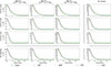 |
Fig. 7. Comparison between the best-fit theoretical predictions of the Compton parameter profiles and the measured data values, for all cluster samples considered in this study. The legend at the bottom specifies the meaning of each plot component. |
A first fit run conducted by letting all parameters free yielded best-fit estimates capable of reproducing the measured profiles within their error bars. However, due to the strong degeneracies existing between model parameters, the posteriors probability distributions appeared broad and poorly constrained, strongly hinting at the possibility of the results being prior driven. This was especially true for the parameter c500, which appeared with error bars in the range 0.2–0.5 over a prior range of 2–3 (depending on the considered model).
To mitigate the effect of parameter degeneracy, a second round of fits was conducted. Initially, c500 was fit alone while all other model parameters were fixed to their best-fit values obtained in the first fit round. Subsequently, these new estimates of c500 were kept fixed while fitting all remaining parameters. This approach noticeably tightened the final constraints and improved the quality of the posterior distributions, as discussed in Sec. 6.1.
Another strong limiting factor to a robust MCMC convergence is the substantial correlation existing between different profile bins, as clearly noticeable in the measured covariance matrices (Fig. 5). These off-diagonal contributions arise from the averaging procedure, smoothing of the maps, and instrumental effects. When combined with the strong parameter degeneracy in a MCMC run, they lead to highly multimodal and unstable posteriors, particularly for the outer radial bins where nominal errors are very small. In the second round of fits, a diagonal-only covariance was then adopted for stability, enabling the robust estimation of the main profile parameters while limiting sensitivity to potentially spurious correlations in the outer bins.
5.3. Results
The resulting parameter best-fit values for all the combinations of model profiles and cluster samples are listed in Tables 2 to 5. In these tables, the values of c500 are those obtained from the fit of the concentration alone, while the values of the remaining parameter are those obtained while keeping c500 fixed. The tables also quote the prior range adopted for each parameter and the final reduced chi-squared values used to assess the goodness of fit. The reduced chi-squared is defined as χr2 = χ2(Θbf)/Nd.o.f., where χ2(Θbf) is the chi-squared derived from Eq. (24) using the best-fit parameter set Θbf, and the number of degrees of freedom Nd.o.f. is computed as the number of fitted data points minus the number of free parameters. These chi-squared values refer to the final fit in which c500 was kept fixed to the tabulated values, and the other parameters were allowed to vary.
Parameter estimation results for the UPP parameterization.
Parameter estimation results for the BMP parameterization.
Parameter estimation results for the PTP parameterization.
Parameter estimation results for the EUP parameterization.
To avoid cluttering the main text, all plots for the posterior distributions on the model parameters are shown separately in Appendix B. A direct comparison between the data and all the best-fit predictions is instead shown in Fig. 7, where for each cluster sample the measured profile points are plotted together with the theoretical profiles. To better show the level of agreement between data and theory, Fig. 8 shows instead the residuals computed as differences between each predicted profile and the measured profile.
A final goal of this study is to assess possible marginal dependencies of the parameters on the chosen mass and redshift bin. To this aim, the best-fit values of the same parameter for different cluster samples are visually compared in Fig. 9. The figure summarizes the constrained magnitudes of all parameters for all theoretical models and is intended to easily reveal the existence of possible trends.
6. Discussion
6.1. About the output of the MCMC runs
An evaluation of the results from the model testing can begin with an overview of the posterior contours shown in Appendix B. The final best-fit values for the concentration c500 are very similar to those obtained in the first fitting round, which is expected since the other parameters were kept fixed. The associated uncertainties, however, became considerably smaller. The final posterior distributions on c500 are shown in Fig. B.1, where all four pressure profile models are overplotted in each data-sample panel. The figure shows that these posteriors are narrow and yield final error bars of order 0.01–0.02; such uncertainties are in fact underestimated, as they arise from the artificially broken degeneracy with the remaining parameters and from the use of diagonalized covariances in the MCMC runs. To provide a more realistic uncertainty estimate, Fisher-matrix errors for c500 were computed using both the full and the diagonal covariance matrices evaluated at the best-fit model. The ratio of these errors defines an inflation factor applied to the MCMC-derived uncertainties. This procedure preserves the best-fit parameter values while restoring an uncertainty that reflects the effective number of independent modes in the full covariance. These corrected uncertainties are those quoted for c500 in Tables 2 to 5. The calculated inflation factors were found in the range 1.1–2.3. Although this confirms the presence of nonnegligible correlations, it does not drastically increase the size of the error bars. In summary, the uncertainties reported for c500, while corrected to provide a more conservative estimate, may still underestimate the fully marginalized constraints that would result from sampling all parameters simultaneously with the full covariance.
The posteriors on the remaining parameters obtained from the last MCMC stage are shown in Figs. B.2 to B.5. For a given pressure-profile model, the contours derived from the different cluster samples exhibit broadly consistent shapes. This is especially true for the BMP and PTP cases, for which only two parameters were fit. The UPP and EUP models, which involve three free parameters, display a larger degree of variation across samples. This behavior reflects the residual parameter degeneracies that remain even in a reduced parameter setting and is particularly evident for the UPP case.
In fact, similar features can be noted in the findings of previous studies that fit the UPP on SZ profiles, as in Gong et al. (2019, Figs. 5 and 7), Planck Collaboration V (2013, Fig. 5), and T23, Figs. 19 to 22, with the latter providing an extensive discussion on this issue. The present study offers an advantage with respect to the UPP-based analysis of T23 by relying on a smaller set of free parameters. Cluster positions in T23 were based on optical data and could be offset from the peak of the SZ signal, thus necessitating fits for two parameters that quantify the statistical properties of such miscentering. This analysis, on the contrary, employs cluster positions determined via matched-filter search directly on ACT co-added maps, which are then expected to be representative of the SZ signal peaks. Furthermore, the theoretical modeling in T23 adopted cluster masses from scaling relations calibrated on WL data. When testing the UPP profile, this required introducing a bias factor to convert masses into the Arnaud et al. (2010) definition, which assumes hydrostatic equilibrium in the ICM. The present study, however, employs the “uncorrected” masses (as quoted in the ACT cluster catalog); therefore, the introduction of the hydrostatic bias is not necessary. The combination of these two reductions in model complexity, together with the effective breaking of the degeneracy with c500, leads to stabler UPP fits in this work compared to the results of T23. In summary, the modest variations observed among the contours in Appendix B are consistent with expectations given the different data samples and profile models.
The shapes of the posterior contours for the UPP model are similar to those shown in Planck Collaboration V (2013) and Gong et al. (2019), although in our case the removal of the degeneracy with c500 shows overall narrower posteriors between the other pairs of parameters. Posteriors obtained for the BMP and PTP pressure profiles show a clear positive correlation between P0 and β in the former, and between P0 and n in the latter. This is expected, as the fitted observable is the LoS-integrated pressure. Hence, steeper profiles (larger β or n) require higher peak amplitudes (larger P0) to yield the same integral over the cluster span. In the case of the UPP or EUP, interpreting degeneracy directions is complicated by the presence of multiple exponents in the functional form. Mild anticorrelation is observed between α and β, which is expected from the UPP functional form with γ fixed. Similarly, a strong anticorrelation is visible between γ and ζ in the EUP, as they both contribute to steepen the profile. For both profile models, the amplitude P0 is generally found to be positively correlated with the “stronger” exponent (β in the UPP, ζ in the EUP) while being anticorrelated with the other.
6.2. About the agreement between theory and data
Fig. 7 shows good agreement between the measured Compton profiles and those predicted theoretically using the best-fit parameters, for all different profile models. Fig. 8 shows the residual differences between predictions and measurements and enables a more detailed view of their level of agreement up to 7′ from the cluster center, which is the effective range employed in the fits. The residual plots confirm a substantial agreement between data and models, with more visible fluctuations near the core where error bars are larger. Once again, such deviations are not unusual in this context: similar deviations have been found in previous fits of pressure profile models against cluster data as in Gong et al. (2019) and T23.
The goodness of fit can be assessed more quantitatively with the χr2 values from Tables 2 to 5. Values depend on the chosen cluster sample but are mostly below unity. In fact, some cases are substantially below unity, hinting at overfitting possibly due to the diagonalization of the covariance. Other cases, instead, denote poorer levels of agreement with the data. This almost always occurs for the intermediate redshift bin, which yields χr2 values mostly above unity. An inspection of Fig. 8 reveals in fact poorer agreement between the fitted curves and data points at large radii (being clearly visible at θ ≳ 5′), signaling that the models struggle to accommodate the Compton profile decrease in the cluster outskirts in this redshift range. Specifically, models in this region tend to underestimate the amplitude, potentially suggesting that even after subtracting the estimated zero-level in each stack, small residual large-scale signals in the maps could still contribute to a modest excess in the outskirts. For all other cases, the χr2 estimates overall confirm the initial assessment that all profile models effectively reproduce the angular dependence of the cluster Compton signal.
Also, there is no compelling indication of which model should be favored; χr2 fluctuations across different cluster samples for the same model profile are larger than average χr2 differences between different models. The goodness of fit, in each case, is mostly determined by the performance of the MCMC in retrieving a global minimum, not by different efficiencies of the underlying theoretical model. The BMP and UPP model could perhaps be deemed the most and least favored, respectively, as χr2 are overall smaller for the former and larger for the latter. This conclusion, however, only holds by a relatively small difference. It is also interesting to notice that the UPP and EUP profiles, despite having one additional free parameter, do not always yield lower χr2 values compared to the BMP and PTP profiles. As discussed, including more parameters in the profile fitting risks increasing model degeneracy, thus making a robust MCMC convergence more challenging.
6.3. About trends in the best-fit parameters
The set of 16 different samples allows us to assess possible residual dependencies of the profile parameters on mass and/or redshift. The error bars quoted in Tables 2–5 indicate that, for the same profile model, best-fit parameters obtained from different data samples can differ beyond the 68% confidence level. This tension likely results from overall underestimated error bars due to the measures implemented to achieve a robust MCMC fitting, as discussed in Secs. 6.1 and 5.2. The variations in best-fit parameter estimates across different mass and redshift bins are visually summarized in Fig. 9, which can also be useful to recognize possible patterns.
The normalization parameter P0 hints at an increase in higher masses and lower redshifts. This is very clear for the EUP model and marginally visible for the UPP model. In the case of the BMP and PTP profiles, a noticeable exception is the highest-mass, highest-redshift bin, whose amplitude is considerably larger than this trend would suggest. The χr2 for this data sample, however, is on the high side compared to the same redshift bin values in Tables 3 and 4, and the error bars quoted on P0 are the highest. Hence, despite being a clear outlier from the proposed trend, this bin also provides looser constraints and lower agreement between theory and data. The work in Gong et al. (2019) also detected a marginal redshift dependence in the profile amplitude, which the author corrected by adding an additional exponent η < 0 to the E(z) factor in Eq. (18), thus mitigating the profile amplitude increase with redshift. The finding in the present study goes in the same direction, favoring a higher normalization for lower redshifts.
As for the other parameters, it is not possible to identify any clear trend for the concentration c500 in any of the considered models. Similar considerations apply to the UPP parameter α and the EUP parameter γ. The slopes UPP β, BMP β, PTP n, and EUP ζ seem to follow a trend similar to the profile normalization (with varying extent depending on the considered model), which can be expected from their positive correlation with P0 as visible in the parameter posterior probability contours. This hints at a steeper profile decrease at higher masses and lower redshifts.
In summary, the observed marginal trends in the amplitude and slope suggest that ICM pressure in the most massive and lowest-redshift clusters has higher peak values and steeper decreases at their outskirts. This finding may indeed have a physical origin: this description fits the most evolved systems that have reached equilibrium (typically cool-core clusters). Conversely, lower-mass and higher-redshift clusters tend to be more disturbed systems, with hot gas more likely spread out by mergers and turbulence (Zhang et al. 2011; Lovisari et al. 2020). In principle, this scenario should result in a similar trend for the concentration, with higher values of c500 at high masses and low redshifts; however, the plots in Fig. 9 show no compelling evidence for this. Once more, this could be a result of parameter degeneracy, as the concentration values are largely determined by the first MCMC round, which fits all parameters simultaneously. In this scenario, the normalization and slope parameters might be “absorbing” the changes in c500, effectively erasing any quantifiable concentration trend in the best-fit estimates.
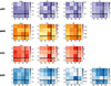 |
Fig. 9. Visual representation of the constrained parameters dependence on the chosen mass and redshift bin. Each row refers to a different theoretical model, and each plot to a specific parameter. Mass and redshift bins are labeled with a number subscript or with “A” for “All”. |
6.4. About the constrained parameter values
To conclude this section, it is worth commenting on the values obtained for individual parameters. Starting from the concentration c500, which is common to all profile models, its best-fit values are generally above 2. In fact, if the calculation of the overdensity radius in Eq. (15) had used the bias-corrected masses from the ACT catalog (on average 30% larger), then the resulting R500 would have been ∼9% larger, and the same increase would have been observed in the best-fit concentration parameters (thus adding one or two decimal units to the retrieved values of c500). Still, this is well within the range covered by estimates from the literature. While lower concentration values were favored in previous studies of the UPP profile (e.g., Arnaud et al. 2010; Gong et al. 2019), other studies adopting either UPP or polytropic functional forms quotes or hints at values of c500 higher than 2 (e.g., Bulbul et al. 2010; McDonald et al. 2014; Ma et al. 2021; Ghirardini et al. 2019; Ettori et al. 2019; Tramonte et al. 2023).
The remaining UPP parameter estimates are in broad agreement with literature findings. Figure 10 shows a direct comparison between the UPP profile ℙ(x) computed using the best fit parameters from this study (for all cluster sample cases) and the same profile computed using the parameters quoted in previous studies. These include the studies by Nagai et al. (2007) and Arnaud et al. (2010), who fit the profile on a reduced sample of high-significance clusters, the study by Ma et al. (2021), who fit the profile on cross-correlations between SZ and lensing data (the latter including both shear and convergence), and the study by T23, who fit the profile on a population-level sample of galaxy clusters using both Planck and ACT maps. The independent variable in the figure is defined as  , where x is the independent variable used so far in this study, in order to include the effect of the concentration parameter from different references. The comparison shows that the predictions obtained with the current analysis are in substantial agreement with the ones from the literature. Some marginal difference can be found in the outskirts, where the profile fit in this study tends to decrease more slowly.
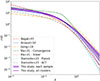 |
Fig. 10. Comparison between the UPP ℙ(x) predictions calculated using the parameters quoted in different studies. For the present study, the solid line shows the prediction from the parameter fit on the full cluster sample, while the shaded region encompasses the predictions from all different samples. |
In the case of the BMP model, the best-fit values for the slope β are in the range [0.9, 1.3]. These are slightly higher than previous estimates based on studies of clusters with X-ray data, typically pointing toward β values in the range ∼0.5 − 0.8 (Birkinshaw 1999; Croston et al. 2008), although values β > 1 have occasionally been reported8 (Ettori 2000; Vikhlinin et al. 2006). The higher slopes obtained in this study might be due to the scaling of the radial separation by the radius rs defined via the concentration parameter c500. The referenced studies, instead, all scaled the separation using the “core” radius of the cluster rc, defined as the very central region of the cluster where its density can be approximated as uniform. There is no fixed relation between R500 and rc in a cluster, with some cases having ratios of a few units and others larger than 10 (Vikhlinin et al. 2006), with higher values typically assigned to relaxed, cool-core systems. In general, it is safe to say that rc < rs is always satisfied. As our BMP model is scaled by rs instead of rc, it is therefore reasonable to expect higher values of β. In fact, the values quoted in Table 3 are not as high as they could be expected from using rs instead of rc. Since β and c500 are expected to be anticorrelated, as they change the profile amplitude in the same direction, it is possible that lower slope values are allowed by the slightly higher concentration estimates obtained for the BMP (c500 ∼ 2.0 − 2.6).
As for the PTP model, the best-fit estimates are also consistent with previous findings. The studies by Eckert et al. (2013) and Ghirardini et al. (2019) point to polytropic index values Γ ∼ 1.2 (more broadly, in the range Γ ∼ 1.1 − 1.3). The latter translates into an exponent n ∼ 5 in agreement with the values listed in Table 4. The study in Ghirardini et al. (2019) also provides constraints on the concentration at c500 ∼ 2.6, supporting the present findings of concentrations c500 > 2.
Finally, the constraints from the EUP model do not have any term of comparison in the literature. It is perhaps worth commenting that the parameter γ was constrained to quite low values (< 1) to mitigate the exponential cutoff of the profile amplitude at large radii. The estimates for the polynomial exponent ζ are instead in between the values constrained for the parameters α and β for the UPP model, hinting at a similar power-law decrease in the intermediate-to-large radial range.
7. Conclusions
This study measured the integrated Compton parameter profile of a population-level sample of 3496 galaxy clusters extracted from the ACT-DR4 catalog by means of stacks on the ACT-DR6 y-map, which covers a sky area of ∼13 000 deg2 with a resolution of 1.6′. The clusters span a mass range [1014,1015.1] M⊙ and a redshift range [0, 2], with mass and redshift each split into three smaller bins to yield nine disjoint cluster subsamples and six subsamples obtained by marginalizing over one variable at a time. For all samples, the averaged Compton parameter profiles were measured with high significance per bin in the range χb2 ∼ 10 − 20.
These profiles were modeled by theoretically integrating the cluster pressure along the line of sight and performing the relevant sample averages. Pressure profiles were modeled in a “universal” approach, whereby the cluster mass and redshift dependence is factorized out as a common factor and the pressure only depends on the separation from the cluster center scaled via a suitable concentration parameter c500. As for the actual pressure profile form, four different models were considered: a gNFW model (UPP), a β-profile model (BMP), a polytropic model (PTP), and a new ansatz including a pressure exponential decay (EUP). Each model came with a different set of free parameters to be constrained against observations. A set of multistage MCMC runs, designed to break the strong degeneracy of the model-specific parameters with c500, was employed to compare the predicted and measured y profiles and reconstruct the posterior probability distribution on such parameters. Best-fit estimates were obtained and tabulated, and the associated predictions were compared to the data.
All models proved effective in reproducing the observed angular dependence of the averaged Compton profiles for all cluster samples, within the error bars. The constrained values of individual parameters were in broad agreement with literature findings. In particular, the predicted UPP pressure profile was found to be compatible with the predictions from previous studies. For a given pressure model, individual parameters were found to exhibit some tension across different cluster samples. The error bars, however, are likely underestimated overall, as a result of the staged MCMC fitting and the removal of correlations in different angular bins implemented to ensure robust convergence. For some parameters these residual dependencies on mass and redshift hinted at an overall trend: high-mass, low-redshift clusters (typically the most dynamically relaxed systems) favor higher amplitudes and steeper profiles than predicted by the universal model.
While similar to the analysis conducted in T23, this study differs in the detailed implementation of the analysis and in its overall goals. The cluster SZ stack in this study was conducted on a more extended y map and employed a refined pipeline, which corrects for the pixel area distortion. Furthermore, this study used a homogeneous cluster sample extracted from ACT co-added maps, unlike the sample in T23, derived from a heterogeneous mix of catalogs based on optical observations. This mitigated the effect of residual biases in the mass definition and allowed us to forego the usage of miscentering parameters in cluster SZ modeling. Furthermore, this study did not employ the hydrostatic mass bias at any point in the analysis, always referring to the SZ-based mass estimates from the catalog. The result is a reduction in the number of free parameters, which helped mitigate degeneracy effects and likely allowed us to detect residual trends in some of their best-fit values. Finally, while T23 only focused on UPP parameterization, this study aimed at comparing the efficiency of different pressure profile models.
Compared to the study of individual and well-resolved clusters, stacks have the advantage of enabling the inclusion of lower mass objects and performing population-level studies, which may highlight possible drifts with the model parameters for different regimes, as indeed proven in the present work. At the same time, however, it has also shown how very different pressure profile parameterizations are almost equally effective in fitting the data. This may suggest that population-level studies of the cluster pressure profile, using SZ data alone, lack the required constraining power to discriminate among competing models. A clear drawback of using either SZ or X-ray cluster data is that the “true,” underlying 3D pressure profile is not directly observable. Measurement always contains LoS-integrated quantities, which enable different functional forms and different parameter combinations, to yield the same prediction. A joint study of both cluster SZ (proportional to the integrated density) and X-ray (proportional to the integrated square of the density) emission could help break the degeneracy, even though it requires a suitable ansatz for the radial temperature dependence. This approach has already been explored (Planck Collaboration V 2013; Sayers et al. 2016), although it has not been applied to a population-level sample.
In this context, while the UPP gNFW parameterization has become a default choice in several astrophysical and cosmological studies involving the ICM profile, there appears to be no substantial reason to prefer it over other, more physically motivated profiles such as the β-model or the polytropic model. While a strongly steep profile in the center may be favored by numerical simulations of dark matter halos Navarro et al. (1997), this has not always been confirmed by observations (Sand et al. 2004; Newman et al. 2013; Li et al. 2023) and, even more so, could not be applicable to the baryonic component. This might be the reason why flatter-core profiles, such as the BMP or the EUP in the present study, are still effective in fitting the measured cluster SZ signal. The usage of the gNFW parameterization can still be justified as a matter of convenience and continuity with previous studies; however, given its ad hoc fitting-oriented nature, and the heavy degeneracies intrinsic to its functional form, any further attempt at constraining its parameter values would not provide any real insight into the physics of the ICM.
On a different note, the marginal dependence of some parameters on cluster mass and redshift challenges the applicability of a universal model assumption. Clusters of galaxies span up to 3 orders of magnitude in mass and are continuously evolving systems, particularly at higher redshifts. While the idea of a common, underlying pressure profile form is theoretically appealing, no universal model would ever be able to exactly capture variations in individual systems or even in different mass and/or redshift regimes – at least not without increasing the number of model parameters to where their individual values lose clear physical meaning. Even the previously cited studies that adopt such physically motivated profiles as the BMP or the PTP, typically use them in combination with others (e.g., gNFW forms) or in more elaborate parameterizations with an extended parameter set. This does not mean, however, that universal forms should be abandoned: they are still capable of capturing average cluster properties with a large range of applicability, and are especially useful in cosmology-oriented studies.
A final conclusion of this work is perhaps that, whenever an analytical description of the ICM pressure is required, a compromise must be reached between modeling precision and the model’s physical interpretability and universality. Future studies can further investigate this tension using increasingly extended datasets. For example, the ACT collaboration has recently announced its largest cluster sample to date (ACT-DES-HSC Collaboration 2025), which is expected to be released publicly as part of data release 6 and can be employed for a natural extension of the present analysis.
Acknowledgments
The author acknowledges financial support from the XJTLU Research Development Fund (RDF) grant with number RDF-22-02-068.
References
- ACT-DES-HSC Collaboration (Aguena, M., et al.) 2025, Open J. Astrophys., submitted [arXiv:2507.21459] [Google Scholar]
- Adam, R., Eynard-Machet, T., Bartalucci, I., et al. 2025, A&A, 694, A182 [NASA ADS] [CrossRef] [EDP Sciences] [Google Scholar]
- Allen, S. W., Evrard, A. E., & Mantz, A. B. 2011, ARA&A, 49, 409 [Google Scholar]
- Arnaud, M. 2009, A&A, 500, 103 [NASA ADS] [CrossRef] [EDP Sciences] [Google Scholar]
- Arnaud, M., Pratt, G. W., Piffaretti, R., et al. 2010, A&A, 517, A92 [CrossRef] [EDP Sciences] [Google Scholar]
- Birkinshaw, M. 1999, Phys. Rep., 310, 97 [Google Scholar]
- Braspenning, J., Schaye, J., Schaller, M., Kugel, R., & Kay, S. T. 2025, MNRAS, 536, 3784 [Google Scholar]
- Bulbul, G. E., Hasler, N., Bonamente, M., & Joy, M. 2010, ApJ, 720, 1038 [NASA ADS] [CrossRef] [Google Scholar]
- Bulbul, E., Liu, A., Kluge, M., et al. 2024, A&A, 685, A106 [NASA ADS] [CrossRef] [EDP Sciences] [Google Scholar]
- Carlstrom, J. E., Holder, G. P., & Reese, E. D. 2002, ARA&A, 40, 643 [Google Scholar]
- Cavaliere, A., & Fusco-Femiano, R. 1976, A&A, 49, 137 [NASA ADS] [Google Scholar]
- Cavaliere, A., & Fusco-Femiano, R. 1978, A&A, 70, 677 [NASA ADS] [Google Scholar]
- Coulton, W., Madhavacheril, M. S., Duivenvoorden, A. J., et al. 2024, Phys. Rev. D, 109, 063530 [NASA ADS] [CrossRef] [Google Scholar]
- Croston, J. H., Pratt, G. W., Böhringer, H., et al. 2008, A&A, 487, 431 [NASA ADS] [CrossRef] [EDP Sciences] [Google Scholar]
- Eckert, D., Molendi, S., Vazza, F., Ettori, S., & Paltani, S. 2013, A&A, 551, A22 [NASA ADS] [CrossRef] [EDP Sciences] [Google Scholar]
- Ettori, S. 2000, MNRAS, 318, 1041 [Google Scholar]
- Ettori, S., Ghirardini, V., Eckert, D., et al. 2019, A&A, 621, A39 [NASA ADS] [CrossRef] [EDP Sciences] [Google Scholar]
- Gallo, S., Douspis, M., Soubrié, E., & Salvati, L. 2024, A&A, 686, A15 [NASA ADS] [CrossRef] [EDP Sciences] [Google Scholar]
- Ghirardini, V., Ettori, S., Eckert, D., & Molendi, S. 2019, A&A, 627, A19 [NASA ADS] [CrossRef] [EDP Sciences] [Google Scholar]
- Gong, Y., Ma, Y.-Z., & Tanimura, H. 2019, MNRAS, 486, 4904 [Google Scholar]
- Goodman, J., & Weare, J. 2010, Commun. Appl. Math. Comput. Sci., 5, 65 [Google Scholar]
- Hartlap, J., Simon, P., & Schneider, P. 2007, A&A, 464, 399 [NASA ADS] [CrossRef] [EDP Sciences] [Google Scholar]
- He, Y., Mansfield, P., Rau, M. M., Trac, H., & Battaglia, N. 2021, ApJ, 908, 91 [NASA ADS] [CrossRef] [Google Scholar]
- Hicks, A. K., Ellingson, E., Bautz, M., et al. 2008, ApJ, 680, 1022 [Google Scholar]
- Hilton, M., Sifón, C., Naess, S., et al. 2021, ApJS, 253, 3 [Google Scholar]
- Kaiser, N. 1986, MNRAS, 222, 323 [Google Scholar]
- Kornoelje, K., Bleem, L. E., Rykoff, E. S., et al. 2025, ApJ, submitted [arXiv:2503.17271] [Google Scholar]
- Kravtsov, A. V., Vikhlinin, A., & Nagai, D. 2006, ApJ, 650, 128 [Google Scholar]
- Li, P., Tian, Y., Júlio, M. P., et al. 2023, A&A, 677, A24 [NASA ADS] [CrossRef] [EDP Sciences] [Google Scholar]
- Lovisari, L., Schellenberger, G., Sereno, M., et al. 2020, ApJ, 892, 102 [Google Scholar]
- Ma, Y.-Z., Gong, Y., Tröster, T., & Van Waerbeke, L. 2021, MNRAS, 500, 1806 [Google Scholar]
- Madhavacheril, M. S., Hill, J. C., Næss, S., et al. 2020, Phys. Rev. D, 102, 023534 [Google Scholar]
- Markevitch, M., & Vikhlinin, A. 2007, Phys. Rep., 443, 1 [Google Scholar]
- McCarthy, F., & Hill, J. C. 2024, Phys. Rev. D, 109, 023528 [Google Scholar]
- McDonald, M., Benson, B. A., Vikhlinin, A., et al. 2014, ApJ, 794, 67 [Google Scholar]
- Mehrtens, N., Romer, A. K., Hilton, M., et al. 2012, MNRAS, 423, 1024 [NASA ADS] [CrossRef] [Google Scholar]
- Miyatake, H., Battaglia, N., Hilton, M., et al. 2019, ApJ, 875, 63 [Google Scholar]
- Nagai, D., Kravtsov, A. V., & Vikhlinin, A. 2007, ApJ, 668, 1 [Google Scholar]
- Navarro, J. F., Frenk, C. S., & White, S. D. M. 1997, ApJ, 490, 493 [Google Scholar]
- Newman, A. B., Treu, T., Ellis, R. S., et al. 2013, ApJ, 765, 24 [NASA ADS] [CrossRef] [Google Scholar]
- Planck Collaboration V. 2013, A&A, 550, A131 [NASA ADS] [CrossRef] [EDP Sciences] [Google Scholar]
- Planck Collaboration XXII. 2016, A&A, 594, A22 [NASA ADS] [CrossRef] [EDP Sciences] [Google Scholar]
- Planck Collaboration XXVII. 2016, A&A, 594, A27 [NASA ADS] [CrossRef] [EDP Sciences] [Google Scholar]
- Planck Collaboration VI. 2020, A&A, 641, A6 [NASA ADS] [CrossRef] [EDP Sciences] [Google Scholar]
- Pointecouteau, E., Santiago-Bautista, I., Douspis, M., et al. 2021, A&A, 651, A73 [NASA ADS] [CrossRef] [EDP Sciences] [Google Scholar]
- Sand, D. J., Treu, T., Smith, G. P., & Ellis, R. S. 2004, ApJ, 604, 88 [NASA ADS] [CrossRef] [Google Scholar]
- Sarazin, C. L. 1988, X-ray Emission from Clusters of Galaxies (Cambridge: Cambridge University Press) [Google Scholar]
- Sayers, J., Golwala, S. R., Mantz, A. B., et al. 2016, ApJ, 832, 26 [Google Scholar]
- Sunyaev, R. A., & Zeldovich, Y. B. 1972, Comments Astrophys. Space Phys., 4, 173 [NASA ADS] [EDP Sciences] [Google Scholar]
- Tramonte, D., Ma, Y.-Z., Yan, Z., et al. 2023, ApJS, 265, 55 [CrossRef] [Google Scholar]
- Vikhlinin, A., Kravtsov, A., Forman, W., et al. 2006, ApJ, 640, 691 [Google Scholar]
- Vikhlinin, A., Burenin, R. A., Ebeling, H., et al. 2009, ApJ, 692, 1033 [Google Scholar]
- Voges, W., Aschenbach, B., Boller, T., et al. 1999, A&A, 349, 389 [NASA ADS] [Google Scholar]
- Voit, G. M. 2005, Rev. Mod. Phys., 77, 207 [Google Scholar]
- Weinberger, R., Ehlert, K., Pfrommer, C., Pakmor, R., & Springel, V. 2017, MNRAS, 470, 4530 [CrossRef] [Google Scholar]
- Zhang, Y. Y., Andernach, H., Caretta, C. A., et al. 2011, A&A, 526, A105 [NASA ADS] [CrossRef] [EDP Sciences] [Google Scholar]
Although a substantial part of the analysis in T23 was dedicated to correcting possible biases from different mass definitions and showing their effects fall largely below the final error bars, that work still acknowledged this as a potential source of systematics.
Although the map is initially apodized, every mask pixel with a value lower than 1 is set to 0.
Notice that for consistency with the mass definition used in this study, the mass in Eq. (15) assumes hydrostatic equilibrium and is thus bias-uncorrected.
Although all the functional forms for ℙ explored in this study are universal (i.e., they lose dependence on the cluster mass and redshift), the term “universal profile” is used only in this particular case to remain consistent with the literature.
These reports, however, refer to extended versions of the β-model, which includes additional parameters, so this comparison is only marginally relevant.
Appendix A: Effect of CIB contamination on the profile reconstruction
Residual contamination from the CIB, a diffuse remnant of various astrophysical processes occurred throughout cosmic history (particularly dust emission and redshifted light from distant galaxies) is a potential source of bias of any analysis based on Compton parameter maps. In order to assess whether the presence of CIB residuals in the ACT DR6 Compton parameter map constitutes a source of significant bias, the same procedure for cluster stacking and profile reconstruction, as described in Sec. 3, was repeated using different versions of the ACT y-map obtained de-projecting the CIB component. As anticipated in Sec. 2.1, the CIB SED is modeled as a modified blackbody, whose functional form includes the CIB temperature TCIB and an emissivity parameter β. Coulton et al. (2024) adopted the fiducial values TCIB = 10.7 K and β = 1.7, as derived in McCarthy & Hill (2024); the previous release of the ACT y-maps (Madhavacheril et al. 2020), instead, adopted the values TCIB = 24 K and β = 1.2.
The ACT-DR6 release includes de-projected maps for different values of the CIB temperature and emissivity; given the existing uncertainty on these parameters, the effect of CIB contaminations on the Compton profiles reconstructed in this study is assessed considering all six combinations for the values TCIB = 10.7 K, 24.0 K and β = 1.0, 1.7, 2.0. For each of these maps and each of the cluster samples considered in this study, the Compton profile yCIB(θ) is reconstructed and compared with the corresponding fiducial profile y(θ); the residuals Δy(θ) = yCIB(θ)−y(θ) are then computed and plotted in Fig. A.1.
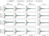 |
Fig. A.1. Effect of CIB contamination on the reconstructed profiles, shown as residuals Δy(θ) between the profiles obtained from the CIB de-projected maps, and the fiducial profiles obtained from the unprojected map. Results are shown for all the 16 cluster samples employed in this study, and for different versions of the CIB de-projected maps (as shown in the legend at the top). The uncertainties associated with the fiducial profiles are also shown as shaded gray regions. |
The figure shows that CIB de-projection does indeed have an effect on the reconstructed profiles, with higher values for the CIB temperature and for the emissivity generally yielding higher y amplitudes (i.e., less contamination). We can also see, however, that these variations are generally within the uncertainties of the unprojected profiles, and while they always result in a decrement at the profile peak, they tend to be centered around the fiducial profiles at higher angular separations. We can also notice that the fiducial CIB parameter values adopted in Coulton et al. (2024) do not correspond to any of the extreme cases, yielding a profile relatively close to the unprojected one. From these considerations, it is possible to conclude that CIB contaminations are not an important source of systematics in this study, and while their presence should be acknowledged, their impact on the final results of the present analysis is expected to be negligible.
Appendix B: Contour plots
This section presents the parameter posterior distributions as obtained from the multistage MCMC runs for all pressure models. As described in Sec. 5.2, an initial MCMC run was launched to obtain a set of baseline best-fit values for all parameters. In the subsequent run, all parameters except c500 were fixed to those baseline values; the resulting 1D posterior distributions on c500 are plotted in Fig. B.1, for all combinations of datasets and pressure profile models. The following figures, instead, show the posterior distributions obtained in the last MCMC run, in which c500 was fixed to its constraints from the previous round, while the other parameters were allowed to vary. In order, results are shown for the UPP (Fig. B.2), the BMP (Fig. B.3), the PTP (Fig. B.4), and the EUP (Fig. B.5) pressure profile models. Given the large number of subsamples and parameters, posterior contour plots are presented in a compact layout; individual panels and labels are best inspected by zooming in on the electronic version.
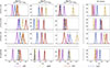 |
Fig. B.1. Posterior 1D probability distributions for the fit on c500, with the remaining parameters fixed. Results are shown for all mass and redshift bins, and for all four models. The vertical dashed lines mark the best-fit values quoted in Tables 2 to 5. |
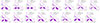 |
Fig. B.2. Posterior contour plots for the parameters entering the UPP model. The dashed lines mark the best-fit values quoted in Table 2. |
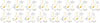 |
Fig. B.3. Posterior contour plots for the parameters entering the BMP model. The dashed lines mark the best-fit values quoted in Table 3. |
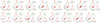 |
Fig. B.4. Posterior contour plots for the parameters entering the PTP model. The dashed lines mark the best-fit values quoted in Table 4. |
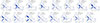 |
Fig. B.5. Posterior contour plots for the parameters entering the EUP model. The dashed lines mark the best-fit values quoted in Table 5. |
All Tables
All Figures
|
Fig. 1. Visual representation of the dataset employed in this study. The ACT DR6 Compton parameter map is plotted on an equirectangular projection – the white region highlighting the mask footprint. The blue spots show the positions of the 4195 clusters from the ACT DR5 catalog. |
| In the text | |
|
Fig. 2. Left and middle panels: distribution in mass and redshift of the full cluster sample adopted in this study. Right: catalog scatter across these two quantities. In all panels, the dashed lines mark the edges of the chosen bins in the corresponding quantity. |
| In the text | |
|
Fig. 3. Summary plot showing the stacks on the ACT y-map of all the 16 cluster samples, described in Sec. 3.1, with labels clarifying the associated mass and redshift intervals. Although the final stack maps are 30′×30′ in size, this figure zooms in on the central 12′×12′ square to better show the details in the cluster signal. |
| In the text | |
|
Fig. 4. Estimation of the mean background level in the stacks. For each mass and redshift bin, the colored bundle represents the set of all 500 profiles extracted from the shuffled stacks. The solid darker line shows their average, taken as the zero-level profile, and the dashed black lines show the 68% confidence interval around the mean. |
| In the text | |
|
Fig. 5. Correlation matrices associated with the reconstructed Compton parameter profiles over the relevant angular span, for all mass and redshift bins. |
| In the text | |
|
Fig. 6. Circularly symmetrized Compton parameter angular profiles extracted from the 16 stacks shown in Fig. 3, background subtracted, and showing the 1-sigma uncertainty per bin as a shaded region. Profiles are grouped according to their mass bin, showing different redshift bins in each panel. The ACT beam profile is included for comparison. |
| In the text | |
|
Fig. 7. Comparison between the best-fit theoretical predictions of the Compton parameter profiles and the measured data values, for all cluster samples considered in this study. The legend at the bottom specifies the meaning of each plot component. |
| In the text | |
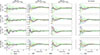 |
Fig. 8. Same as in Fig. 7, but showing residuals Δy between theoretical predictions and data values. |
| In the text | |
|
Fig. 9. Visual representation of the constrained parameters dependence on the chosen mass and redshift bin. Each row refers to a different theoretical model, and each plot to a specific parameter. Mass and redshift bins are labeled with a number subscript or with “A” for “All”. |
| In the text | |
|
Fig. 10. Comparison between the UPP ℙ(x) predictions calculated using the parameters quoted in different studies. For the present study, the solid line shows the prediction from the parameter fit on the full cluster sample, while the shaded region encompasses the predictions from all different samples. |
| In the text | |
|
Fig. A.1. Effect of CIB contamination on the reconstructed profiles, shown as residuals Δy(θ) between the profiles obtained from the CIB de-projected maps, and the fiducial profiles obtained from the unprojected map. Results are shown for all the 16 cluster samples employed in this study, and for different versions of the CIB de-projected maps (as shown in the legend at the top). The uncertainties associated with the fiducial profiles are also shown as shaded gray regions. |
| In the text | |
|
Fig. B.1. Posterior 1D probability distributions for the fit on c500, with the remaining parameters fixed. Results are shown for all mass and redshift bins, and for all four models. The vertical dashed lines mark the best-fit values quoted in Tables 2 to 5. |
| In the text | |
|
Fig. B.2. Posterior contour plots for the parameters entering the UPP model. The dashed lines mark the best-fit values quoted in Table 2. |
| In the text | |
|
Fig. B.3. Posterior contour plots for the parameters entering the BMP model. The dashed lines mark the best-fit values quoted in Table 3. |
| In the text | |
|
Fig. B.4. Posterior contour plots for the parameters entering the PTP model. The dashed lines mark the best-fit values quoted in Table 4. |
| In the text | |
|
Fig. B.5. Posterior contour plots for the parameters entering the EUP model. The dashed lines mark the best-fit values quoted in Table 5. |
| In the text | |
Current usage metrics show cumulative count of Article Views (full-text article views including HTML views, PDF and ePub downloads, according to the available data) and Abstracts Views on Vision4Press platform.
Data correspond to usage on the plateform after 2015. The current usage metrics is available 48-96 hours after online publication and is updated daily on week days.
Initial download of the metrics may take a while.