| Issue |
A&A
Volume 707, March 2026
|
|
|---|---|---|
| Article Number | A388 | |
| Number of page(s) | 27 | |
| Section | Extragalactic astronomy | |
| DOI | https://doi.org/10.1051/0004-6361/202557025 | |
| Published online | 25 March 2026 | |
Investigating the origin of radio emission in candidate super-Eddington accreting black holes
1
Instituto de Astrofísica de Andalucía, Glorieta de Astronomía, Granada IAA-CSIC, Spain
2
Département de physique, de génie physique et d’optique, Université Laval, Québec, (QC), G1V 0A6, Canada
3
Istituto Nazionale di Astrofisica, Osservatorio di Padova, Vicolo dell’Osservatorio 5, 35122, Padova, Italy
4
European Southern Observatory (ESO), Alonso de Córdova, 3107, Casilla 19, Santiago 19001, Chile
5
Department of Physics and Astronomy, Texas Tech University, Box 41051, Lubbock 79409-1051, TX, USA
6
Institute of Physics, Laboratory of Astrophysics, École Polytechnique Fédérale de Lausanne (EPFL), Observatoire de Sauverny, Versoix CH-1290, Switzerland
7
Dipartimento di Fisica e Astronomia “G. Galilei”, Università di Padova, Vicolo dell’Osservatorio 3, 35122, Padova, Italy
8
Istituto Nazionale di Astrofisica, Osservatorio di Cagliari, Via della Scienza 5, 09047, Selargius, Italy
9
Max-Planck-Institut für Radioastronomie, Auf dem Hügel 69, 53121, Bonn, Germany
10
ICRA, Physics Department, University La Sapienza, Roma, Italy
★ Corresponding author: This email address is being protected from spambots. You need JavaScript enabled to view it.
Received:
28
August
2025
Accepted:
26
January
2026
Abstract
Context. Recent studies show that the radio power of quasars accreting at very high rates can reach surprisingly high values. These studies suggest that this radio emission could originate from star formation (SF); however, the lack of data does not rule out the presence of a jetted active galactic nucleus (AGN).
Aims. We investigated the origin of the radio emission of a sample of 18 super-Eddington candidates, over a wide range of redshifts. These sources are expected to have an extreme radiative output per unit black hole mass, show high-velocity outflows, and are therefore thought to be prime mover of galactic evolution via radiative and mechanical feedback.
Methods. We present new Karl G. Jansky Very Large Array (VLA) observations at the L, C, and X bands of these sources, which we combined with observations from the LOw-Frequency ARray (LOFAR) Two-meter Sky Survey (LoTSS) and the Very Large Array Sky Survey (VLASS). We also used optical and IR data to derive estimates of accretion and wind parameters, as well as star formation rates (SFRs), which we compared with those derived from the radio emission.
Results. Based on radio variability, luminosity, morphology, radio spectral properties, radio versus IR estimates of SFR, and radio-to-mid IR flux ratio, we find that seven of our 18 targets likely have radio emission predominantly arising from SF, six from a combination of SF and AGN-related mechanisms, and only three from a core or jetted AGN origin. This result is consistent with previous studies and supports the prevalence of lower-power radio structures associated with star-forming activity rather than relativistic jets in the high Eddington ratio regime. In the same sample, however, the data suggest that three sources simultaneously exhibit super-Eddington accretion and relativistic ejections.
Key words: galaxies: jets / quasars: general / galaxies: star formation
© The Authors 2026
 Open Access article, published by EDP Sciences, under the terms of the Creative Commons Attribution License (https://creativecommons.org/licenses/by/4.0), which permits unrestricted use, distribution, and reproduction in any medium, provided the original work is properly cited.
This article is published in open access under the Subscribe to Open model. This email address is being protected from spambots. You need JavaScript enabled to view it. to support open access publication.
1. Introduction
The main sequence (MS) of quasars is a classification scheme based on their spectral properties, most commonly represented by the plane of the intensity ratio RFeII = W(Fe IIλ4570)/W(Hβ) (where W(Fe IIλ4570) is the equivalent width of the multiplet mix between 4434 Å and 4684 Å and W(Hβ) the equivalent width of the broad component of the Hβ emission line) and the full width at half maximum (FWHM) of the Hβ emission line. It is a powerful tool for analyzing the observational properties of type 1 active galactic nuclei (AGNs; e.g., Sulentic et al. 2000a; Marziani et al. 2018). The MS is relevant for quasar astronomy because several observational and physical properties, such as the prominence of outflows and the prevalence of jetted sources, change systematically along it. There is a growing consensus that the main factors shaping the MS are the Eddington ratio (L/LEdd) and the viewing angle, defined as the angle between the line of sight and the AGN symmetry axis (e.g., Panda et al. 2019). Quasars can be divided into two broad populations based on their position in the MS: population A (narrower Hβ lines, with FWHM < 4000 km s−1) and population B (broad Hβ lines, with FWHM > 4000 km s−1). The subpopulation of quasars located toward the high RFeII end of the MS, called the extreme population A (xA), is characterized by extreme observational parameters and is linked to a high Eddington ratio (Marziani & Sulentic 2014; Du et al. 2016). They exhibit a distinctive UV spectrum that makes them easily recognizable even at high redshift (Martínez-Aldama et al. 2018). The highest radiators per unit mass should be preferentially found at high redshift. Indeed, the most luminous, intrinsically blue composite spectra of the quasar population closely resemble the UV spectra of the highest radiators at low and moderate redshifts (Nardini et al. 2019). They are believed to be in an early stage of evolution (Mathur 2000), and may constitute the dominant source of ionizing photons in the reionization epoch.
A recent analysis shows that radio powers can reach surprisingly high values in xA objects (Ganci et al. 2019), with some entering the radio-loud (RL) regime, defined by Kellermann’s parameter (the ratio Rk between radio flux density at 5 GHz and the optical flux density at 5100 Å; Kellermann et al. 1989), above ten. The strong radio emission from RL sources is typically associated with the presence of a relativistic jet, whereas in radio-quiet (RQ) sources the jet is expected to be nonrelativistic or intrinsically weaker. Star formation (SF) is considered an important contributor, especially at lower powers and frequencies: the fraction of star-forming galaxies increases at fluxes below S1.4 GHz ≃ 10 mJy (e.g., Condon 1989; Smolcic et al. 2017; Mancuso et al. 2017), although other mechanisms more closely related to the AGN have been proposed.
The sample of strong FeII emitters from (Ganci et al. 2019) has high radio powers. Nevertheless, they obey the far-infrared (FIR)-radio correlation for star-forming galaxies and RQ quasars. Moreover, a large fraction (75%) of RL narrow-line Seyfert 1 galaxies (RL NLSy1s) shows mid-IR emission properties consistent with SF being the dominant contributor to radio emission (Caccianiga et al. 2015; Järvelä et al. 2022). Therefore, it is reasonable to suggest that the radio emission from most sample sources in the Ganci et al. (2019) sample is dominated by processes that are not related to AGNs. Nevertheless, the lack of data leaves open the possibility that sources could also harbor a relatively low radio-power relativistic jet or outflow. This scenario applies to sources with relatively low black hole mass, as jet power scales nonlinearly with black hole mass (Heinz & Sunyaev 2003). Indeed, in recent years, a number of objects characterized by prominent FeII emission and formally classified as RQ have been shown to be jetted (e.g., Lähteenmäki et al. 2018; Berton et al. 2018, 2020; Järvelä et al. 2021; Marziani et al. 2021; Vietri et al. 2022).
Among the RL sources from the Ganci et al. (2019) sample, Mrk 231, is a low-z, high-luminosity prototypical xA source. Sulentic et al. (2006) described Mrk 231 as a high-luminosity, highly accreting quasar misplaced at late cosmic epochs. Its emission line properties are extreme in terms of FeII emission, the CIVλ1549 blueshift, and the blueward asymmetry of Hβ. It is a broad absorption line (BAL) quasar that suffers some internal extinction and shows extreme absorption troughs in radial velocity (Sulentic et al. 2006; Veilleux et al. 2016). The unresolved core of Mrk 231 was found to be highly variable and to have a high brightness temperature (Condon et al. 1991). Superluminal radio components have been detected in Mrk 231, along with relation between BALs, radio ejections, and continuum change (Reynolds et al. 2017), illustrating the complex interplay between thermal and nonthermal nuclear emission that is perhaps typical of sources accreting at extremely high rates. Nevertheless, according to the location in the diagram of Ganci et al. (2019), the dominant emission mechanism is SF. This inference is consistent with the enormous CO luminosity of its AGN host (Rigopoulou et al. 1996).
Notwithstanding Mrk 231, the vast majority of extreme radiators remain poorly studied, especially their radio properties. Strong FeII emitters have a high accretion rate, possibly at super-Eddington levels (Du et al. 2016), although their radiative output is expected to remain within a factor ∼2 above the Eddington limit (Mineshige et al. 2000). High L/LEdd can coexist with powerful jetted radio emission (log Pν > 1031 erg s−1 Hz−1). There is no physical impossibility in this respect (Czerny et al. 2018), and recent studies consider the relativistic jet and nonrelativistic wide angle outflows as two aspects of a hydromagnetically driven wind (Reynolds et al. 2017). Concomitant high accretion and high radio power are observed in compact steep-spectrum (CSS) radio sources (e.g., Wu 2009). General relativistic magnetohydrodynamic simulations can also reproduce high L/LEdd sources with jets (McKinney et al. 2017; Liska et al. 2022). Our view is likely biased by the relative rarity of these sources at low-z (O’Dea 1998), especially by the scarcity of high-quality UV and optical spectra, and by their rather preliminary interpretation that, in the past, ignored the MS trends. The basic question is whether the RL sources in the xA spectral bins of the MS are truly jetted (as RL NLSy1s are; Foschini et al. 2015) or are dominated by radio emission from SF.
Generally, RL extreme accretors may appear indistinguishable in the Hβ spectral range from their RQ counterparts, as both RQ and RL strong-FeII emitters show a large blueshift in their [O III] profiles (Berton et al. 2016; Berton & Järvelä 2021). The radio power may be associated with a relatively small black hole mass. They could represent systems in an early evolutionary stage, with spin-up enabled by a recent accretion event (Mathur 2000; Sulentic et al. 2000a), but the possibility of radio emission from SF calls into question the role of radio-mode AGN feedback as a cosmologically relevant process in massive galaxy formation. This class of sources is believed to represent highly accreting quasars observed at very early cosmic epochs, as demonstrated by the NLSy1-like object recently discovered at z = 6.56 (Wolf et al. 2023). Sources in the reionization epoch may accrete at super-Eddington rates, with their associated starbursts serving as the primary source of ionizing photons (e.g., Decarli et al. 2017). Several of the highest-redshift quasars have been detected in the radio, implying extremely powerful radio emission (e.g., Belladitta et al. 2019). However, it remains unclear which mechanism dominates: SF or black hole activity. Establishing their relative contributions in high accretors is expected to provide strong constraints on the ability of nuclear activity to serve as the main source of ionizing photons during the reionization epoch.
In this work, we analyze the observations carried out with the Karl G. Jansky Very Large Array (VLA) of a sample of 18 xA sources with intensity ratio RFeII ≳ 1 from Marziani et al. (2003), Sani et al. (2010) and Ganci et al. (2019). We supplement these with radio survey observations, as well as optical and IR data, to determine the origin of the radio emission. Section 2 presents the sample and the data reduction process, while Section 3 presents the analysis of these datasets. We discuss our findings in Section 4 and summarize our results in Section 5. Appendix C presents an analysis of optical and IR data relevant for interpreting the radio observations. We adopt H0 = 70 km s−1 Mpc−1, ΩM = 0.3, and Ωvac = 0.7.
2. Sample selection and data reduction
Table 1 presents our complete sample and contains a total of 18 sources, the optical spectra of which are classified as xA objects in the MS (i.e., RFeII ≳1). Throughout the paper, we refer to the sources by their short names as listed in column 2 of Table 1. We emphasize that this condition is thought to be associated with black holes exhibiting the highest radiative output per unit mass (e.g., Marziani et al. 2001; Sun & Shen 2015; Du et al. 2016; Panda et al. 2019; Marziani et al. 2025). Among these sources, several show multifrequency evidence of extraordinary activity levels, which may indicate super-Eddington accretion (Marziani et al. 2025, and references therein). Five of these sources were taken from the radio survey of Ganci et al. (2019), with the remainder supplemented by low-z sources from Sani et al. (2010) and Marziani et al. (2003) detected in FIR.
Sample targets.
In optically selected quasar samples, RL sources tend to concentrate at the extremes of the MS. Figure 1 shows the incidence and radio power as a function of spectral type along the quasar MS for the sources detected by FIRST in the sample of (Marziani et al. 2013). Most powerful radio sources are found among B spectral types; when observed pole-on, they appear core-dominated with narrower lines, allowing them to populate part of spectral type A1 (Wills & Browne 1986; Jarvis & McLure 2006; Ganci et al. 2019). Surprisingly, xA spectral types show a threefold increase in the prevalence of radio-detected sources, but with a systematically lower radio power.
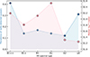 |
Fig. 1. Prevalence of FIRST-detected type 1 AGNs (Marziani et al. 2013) (blue circles and cyan shading) and median radio power (red circles and pink shading) as a function of spectral type along the quasar main sequence. |
Radio emission properties found in one domain, such as the xA regime defined by RFeII ≳ 1 (spectral types A3 and A4; see Sulentic et al. 2002), can be generalized to other sources with similar spectral characteristics. However, these results do not extend to quasars with markedly different spectral types along the MS, particularly those at the extreme end of population B. In simple terms, population B sources may exhibit radio power comparable to xA quasars, yet the origin of that radio emission could be fundamentally different, most likely jet-driven (Zamfir et al. 2008; Ganci et al. 2019).
An additional consideration in interpreting these data concerns the spatial origin of the FIR emission. Relativistic jets are nuclear phenomena, and the presence of radio lobes corroborates jet activity, whereas SF can be nuclear, circumnuclear, or distributed across the host. Because the available measurements do not spatially resolve the FIR emission attributed to SF, we cannot exclude a contribution from a mildly beamed (i.e., weakly Doppler-boosted) or misaligned relativistic jet.
2.1. VLA data
We obtained the radio observations from the VLA project 20B-081 (PI: M. Berton). These comprise 17 datasets, each including a single target, except one dataset containing two sources, J1209+5611 and J1301+5902. All observations were carried out from 4 December 2020 to 8 December 2020 in three bands: L (1.5 GHz), C (5 GHz), and X (10 GHz). Due to the COVID pandemic, the data were taken in a nonstandard configuration, with two arms fully extended in the A-configuration and one arm in the more compact B-configuration, except for one antenna moved to the end of the arm. Fig. A.2 shows the antenna positions during the observations of J00418+4021 on 4 December 2020, along with the associated uv plane coverage of the L-band scan. This nonuniform configuration may have slightly affected the image quality, producing a slightly elongated synthesized beam; however, the overall impact appears negligible, as the rms noise is consistent with the expected values. We used 8-bit samplers for the L band, with center frequencies of 1.25 and 1.75 GHz; for the C band, 8-bit samplers centered at 4.72 and 5.75 GHz; and for the X band, two 3-bit samplers centered at 9 and 11 GHz. Each target was observed for a total of 10 minutes per band, which, accounting for amplitude and phase calibration and overheads, corresponded to 20 minutes per band.
We applied the CASA (Casa et al. 2022) pipeline version 6.4.1.12 to each dataset. We visually inspected the outputs to ensure that the pipeline performed well on all datasets. After calibration, the target observations for each band were split into individual measurement sets. We did not perform any (time or frequency) averaging. We individually imaged each dataset using TCLEAN in CASA (version 6.5.2.26). We used two Taylor coefficients to model the spectral structure of the emission across each band and applied W-projection corrections with 14, 4, and 2 planes, for the L, C, and X bands, respectively, to correct for the wide-field noncoplanar baseline effect (Cornwell et al. 2008). We adopted cell sizes of 0.2″, 0.07″, and 0.03″ for the L, C, and X-band images, respectively, and image sizes of 9000 pixels × 9000 pixels = 30′×30′, 7500 pixels × 7500 pixels = 8.75′×8.75′, and 9000 pixels × 9000 pixels = 4.5′×4.5′ (approximate sizes of the FWHM of the field of view at the respective frequencies). Due to the presence of very bright sources near J11292–0424, J15455+4846 and J17014+5149, we increased the size of the L-band image, which significantly improved the image quality. We used the multi-scale CLEAN algorithm from Cornwell (2008) with scales of 0, 5, and 15 pixels to probe structures on different scales. We applied Briggs weighting with a robust factor of 0.5, an intermediate between natural and uniform weighting. We performed a round of phase self-calibration to improve the overall dynamic range for J11292–0424, whose field encompassed the brightest source, and for 12562+5652, which is the brightest target. Finally, we calculated wideband primary beam corrections with the CASA task WIDEBANDPBCOR, listing all the spectral windows and the middle channel. Fig. A.1 shows cutouts of the final images, and Table B.1 lists the obtained beam sizes, rms, and dynamic ranges (DRs). The noise level in each image was evaluated by averaging the rms noise in the four corners of the cutouts, i.e., near the sources but in regions free of other bright radio sources. On average, the rms values are ∼30, 10, and 8 μJy/beam for the L-, C-, and X-band images, respectively (which are close to the noise expected for such observations based on the VLA exposure calculator), except for J12562+5652, whose brightness limits the noise reachable. Table B.2 lists flux densities enclosed within 5σ contours (or peak flux densities for compact sources). To test the robustness of these measurements, we compared them with integrated flux densities derived from 2D Gaussian fits. We used the CASA task IMFIT for this test and obtained values within ±5% from the 5σ-contour method for sources with an elliptical morphology, confirming the validity of this approach. For flux calibration, we assumed a relative error of 5% for all VLA bands1. The uncertainties were then calculated as the sum in quadrature of the rms and the calibration error. Of the 18 sources observed with the VLA, 17 are detected at X band and 16 at L and C bands. For undetected sources, we report 5σ upper limits in Table B.2.
2.2. Complementary radio data
To complement our VLA observations, we included radio observations from the LOw-Frequency ARray (LOFAR) Two-metre Sky Survey (LoTSS) DR2 (Shimwell et al. 2022) and the Very Large Array Sky Survey (VLASS) (Lacy et al. 2020). We searched for our sources in LoTSS DR2 by first identifying the full-bandwidth Stokes I continuum mosaic (with a central frequency of 144 MHz) that best covers each target and downloaded the corresponding fits file at full resolution. Fig. A.1 shows cutouts around these sources, while the beam sizes, rms, and DRs of the mosaic are listed in Table B.1. We determined the noise level in the same way as for the VLA images, by averaging the rms noise in the four corners of the cutouts. The LOFAR images have beam sizes of 6″ × 6″ and an average noise of approximately 0.1 mJy/beam. We detected all ten sources covered by LoTSS DR2. Table B.2 lists flux densities enclosed within 5σ contours (or peak flux densities for spatially unresolved sources). We assumed a relative flux calibration error of 10% (Shimwell et al. 2022), and we calculated the uncertainties as the sum in quadrature of the rms and the calibration error.
We obtained the VLASS images (central frequency 3 GHz) covering our sources through the Canadian Astronomy Data Centre (CADC) portal. All sources are covered by the survey, in either quick look (QL) or single epoch (SE) continuum images, in at least two epochs. We selected SE images, when available, to extract fluxes, as they serve as the reference continuum images for each VLASS epoch; otherwise, we used the QL image from the epoch closest in time to the VLA observations (see column 8 of Table B.1). The images have beam sizes of approximately 2 − 4″ and an average noise of about 0.1 mJy/beam. Table B.2 lists flux densities encompassed within 5σ contours (or peak flux densities for spatially unresolved sources). We assumed flux calibration relative errors of 3% for SE images and 10% for SE and QL images, with uncertainties calculated as the sum in quadrature of the rms and the calibration error. We also extracted flux from all epochs and plotted each source’s flux variation in Fig. A.3. For sources detected in at least two epochs, we computed the variability index using the formula from Aller et al. (1992),
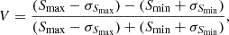 (1)
(1)
where Smin and Smax are the maximum and minimum values of the flux density over all epochs of observations, and σSmin and σSmax are their associated errors. Fig. A.3 shows the resulting variability indices. Negative values of V correspond to cases in which the error is greater than the observed scatter of the data. Three sources exceed V = 0.1, which makes them potential candidates for variable objects (e.g., Kunert-Bajraszewska et al. 2025): J12091+5611, J12562+5652, and J15455+4846. For these sources, the SE flux was adopted for the subsequent analysis, and we verified that it corresponds to the epoch closest in time to the VLA observations.
2.3. Optical and IR data
The optical data are from three main sources: the Marziani et al. (2003) atlas of low-z type 1 AGNs covering the Hβ spectral range; the Marziani et al. (2022) comparative analysis, in which the Hβ spectral range is paired with the rest-frame UV blend at λ1900; and the SDSS. In addition, the spectrum of J00418+4021 was digitized from a published plot (Halpern & Oke 1987). The continuum signal-to-noise ratio (S/N) is ≳20 excluding J00418+4021. The spectral resolution is λ/δλ ∼ 2000 for the SDSS data and λ/δλ ∼ 1000 for the other spectra. We fit the SDSS and Marziani et al. (2003) spectra using the same multicomponent, nonlinear analysis used in Marziani et al. (2022). We paid particular attention to fitting the [O III]λλ4959,5007 lines, as well as to detecting a possible blueshifted (outflow) component in Hβ. Appendix C reports the results of a multicomponent nonlinear analysis of the Hβ and [O III]λ5007 lines, plus accretion parameters (Eddington ratio and black hole mass estimates derived from optical spectra).
We used IR fluxes extracted from the Wide-field Infrared Survey Explorer (WISE; Wright et al. 2010), as well as FIR fluxes from the Infrared Astronomical Satellite (IRAS) survey (Neugebauer et al. 1984), except for J14063+2223, which lacks IRAS data at 100 μm; for this source, we used the flux from the Infrared Space Observatory (ISO) survey (Kessler et al. 1996). Table B.3 lists the IR and FIR fluxes used in the analysis. We also considered data from AKARI (Murakami et al. 2007), ISO, Spitzer MIPS, and Herschel. The AKARI 60 μm fluxes are available only four objects (listed in Table 1), and are ≈20% lower than the IRAS fluxes, as expected from comparisons with more precise data from newer telescopes (Serjeant & Hatziminaoglou 2009). Therefore, we expected the SFR to be consistent with those derived from IRAS data, assuming the same normalization used in Section 3.4.
3. Results
3.1. Radio loudness
We calculated the Kellermann parameter RK (Kellermann et al. 1989), using the radio flux density at 1.4 GHz and the optical flux density at 5100 Å from the second column of Table C.1. The observed radio flux density fν, o reported in Table B.2, was converted to the rest frame by applying a K-correction, fν, e = fν, o[(1 + z)( − α + 1)] (Ganci et al. 2019), where the spectra index α is reported in the sixth column of Table B.4. We classified sources as RL when RK ≥ 10 and as RQ when RK < 10, where RK is computed from the 1.4 GHz radio fluxes reported in Table B.2 and the optical fluxes at 5100 Å (Appendix C). Applying this criterion to our sample yields a large fraction of RL sources (eight out of 18). However, we note that RK ≥ 10 is not, by itself, a sufficient condition to demonstrate the presence of a relativistic jet, especially among xA quasars (Zamfir et al. 2008; Ganci et al. 2019). Using a more restrictive condition, log RK ≥ 1.8 (i.e., RK ≥ 70), as suggested by Zamfir et al. (2008) for the lower boundary of the RL phenomenon when analyzing FRII sources, we would classify only J00418+4021 and J14258+3946 as RL. We also note that the optical continuum of J00418+4021 may be underestimated, which would make J14258+3946 the sole bona-fide RL source in the sample.
3.2. Radio morphology
Following Berton et al. (2018), we define three morphological classes reflecting the properties of the sources seen in the maps, using the ratio (ℛ) of the peak to the total flux density of each source:
-
Compact: sources with ℛ ≥ 0.95, labeled as C in Table B.2
-
Intermediate: sources with 0.75 ≤ ℛ < 0.95, labeled as I in Table B.2.
-
Extended: sources with ℛ < 0.75, labeled as E in Table B.2.
Most sources in our sample are compact; however, at the lowest frequency band (LOFAR data) a much higher fraction of the sources are extended (60% at 144 MHz versus 11% at 1.5 GHz, 17% at 3 GHz, 11% at 5 GHz, and 11% at 10 GHz, respectively).
Overall, only three targets show clear extended emission at most frequencies: J00418+4021, J12562+5652, and J17014+5149. J00418+4021 and J12562+5652 exhibit faint diffuse emission, especially visible at lower frequencies, surrounding their bright core. In contrast, the radio emission of J17014+5149 resolves into two distinct point-like sources at high frequency.
Figure 2 presents the distribution of radio morphologies detected across the various redshifts of our sources. Extended emission is detected even among our highest-redshift sources. At the highest redshift (0.75, J12075+1506), the highest-resolution images resolve structures down to 2–3 kpc, sufficient to resolve relativistic jets or SF regions.
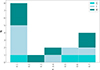 |
Fig. 2. Radio morphology distribution across source redshifts. The letter C indicates compact emission at all observed frequencies, I indicates intermediate morphology detected in at least one band, and E indicates the presence of diffuse emission in at least one band. |
3.3. Radio spectral index
Multifrequency radio observations allow us to precisely measure the spectral index, which helps to determine the origin of the radio emission. We adopt Sν ∝ να, where α is the spectral index. We measured the spectral index between bands as follows:
 (2)
(2)
where S1 and S2 are the flux densities at the observing frequencies ν1 and ν2, respectively. To determine the global spectral index across the available frequency range, we fit the fluxes using NUMPY.POLYFIT for sources with detection in at least three bands. We calculated the uncertainties in the spectral indices using standard error propagation. Table B.4 lists all the spectral indices and Fig. B.1 shows the spectrum of each source detected in at least three bands. Among the three sources exhibiting significant variability in VLASS observations, the flux from J12562+5652 in the nonsimultaneous observations at 144 MHz and 3 GHz falls outside the fitted spectral slope.
For the few sources that showed extended emission at lower frequencies, the large mismatch in resolution with higher-frequency images prevented a spatially resolved analysis of the spectral index. In the case of J17014+5149, where two distinct point-like sources are resolved at C and X bands, we calculated the spectral indices of each point-like source. We used the CASA task IMSMOOTH to smooth the X-band image to the C-band beam (which has the lowest spatial resolution) and then applied the CASA task IMREGRID to regrid the X-band image using the C-band image as a reference. We extracted fluxes from both point-like sources and obtained identical values within the uncertainties of α5 − 10 = −1.0 ± 0.1. This result is consistent with the spectral index calculated from the integrated flux of the sources.
A common approach for characterizing radio spectra involves the use of radio color-color diagrams. Figure 3 shows the spectral indices in the following pairings: α0.144 − 1.5 versus α1.5 − 3, α1.5 − 3 versus α3 − 5, and α3 − 5 versus α5 − 10. To mitigate the effects of nonsimultaneous observations, missing LOFAR images, and VLASS nondetections, we also show a color-color diagram including only the L, C, and X-band VLA observations: α1.5 − 5 versus α5 − 10 in Figure 3. No sources show ultra-steep drop-offs (blue region, Figure B.1, right panel), which would indicate relic emission caused by significant cooling since the last AGN activity, leading to a spectrum with exceptional steepening (α < −2) at high frequencies. This result is consistent with Fraix-Burnet et al. (2017), in which xA sources are interpreted as AGNs in an early evolutionary stage.
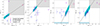 |
Fig. 3. Spectral indices plotted as α1.5 − 5 vs. α0.144 − 1.5, α3 − 5 vs. α1.5 − 3, α5 − 10 vs. α3 − 5, and α5 − 10 vs. α1.5 − 5. Markers are colored according to the dominating mechanism responsible for the detected radio emission (Table 2). The dashed line indicates the 1 : 1 ratio of equal slopes, while the horizontal and vertical dotted lines correspond to α = −0.5. The region showing flat or inverted spectra, which may be associated with a core-dominated jet or a corona, is shaded gray. The region with a spectral index α = −0.8 ± 0.4 and a scatter of 0.2, possibly related to SF, is shaded turquoise. The region showing very steep spectral slopes with α5 − 10 < −2 in the right-hand panel, which may imply possible relic emission, is shaded blue. |
We calculate the radio luminosities of the detected sources using
 (3)
(3)
where L1.4 GHz is the radio luminosity (W Hz−1) at 1.4 GHz, DL is the luminosity distance (Mpc) calculated with Astropy using the redshifts in Table 1, α is the fit spectral index, and S1.4 GHz is the integrated radio flux density at 1.4 GHz extrapolated using the fitted spectral index. These luminosities are reported in Table B.4.
The radio-to-mid IR flux ratio is a useful tool to identify the source of radio emission since it differs significantly for jet-dominated AGNs (i.e., blazars) and star-forming galaxies. Following Caccianiga et al. (2015), we calculated the two-point spectral index between 1.5 GHz and 22 μm, defined as
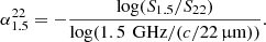 (4)
(4)
Here, S22 is the 22 μm flux density, plus the Q22 parameter, defined as
 (5)
(5)
Blazars, in which the radio emission is dominated by the relativistic jet, exhibit steep  indices, whereas star-forming IR galaxies have
  , with SF as the main contributor to the radio emission Caccianiga et al. (2015). Fig. 4 shows the distribution of radio-to-mid-IR flux ratios for the detected sources. All sources have
  below ∼ − 0.1 except for two: J12091+5611 (
 = 0.02) and J14258+3946 (
 = 0.16). The distribution is narrower than that reported in Caccianiga et al. (2015). We find only a few objects with intermediate values: J12091+5611 (
 = 0.02), J12366+5630 (
 = –0.14), and J14475+3455 (
 = –0.16). For these sources, the radio emission most likely arises from a combination of jet and SF.
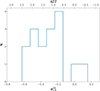 |
Fig. 4. Two-point spectral index between radio (1.4 GHz) and mid-IR (22 μm). All sources have |

The flux densities at 22 μm measured for our sources, we used to derived the Q22 parameter, could be affected by broad emission bands from polycyclic aromatic hydrocarbon (PAH) molecules. The PAH bands are tracers of SF activity, and the 11.3 μm feature is believed to remain a tracer even in the presence of an AGN (Diamond-Stanic & Rieke 2012). Given the redshifts of our sample, the Q22 parameter could be primarily affected by the relatively weak PAH feature at ≈17 μm (Smith et al. 2007). With a typical observed-frame equivalent width of ∼0.5 Å, this feature is expected to contribute slightly more than ∼10% to the total flux in the S22 band. Polycyclic aromatic hydrocarbon (PAH) features are also expected to be fainter in type 1 AGNs, due to dilution or destruction by the AGN radiation field (Xie & Ho 2022). A systematic analysis of the MIR properties of the present sample would be valuable, given the mixed nature of these sources, but is beyond the scope of the present work. However, we used Q22 not as an SF diagnostic but to identify excess radio emission that lowers Q22 and increases  . We therefore classify the two sources in the blazar domain (i.e., with
  ) as dominated by a radio core or jet.
3.4. Star formation estimates
We estimated star formation rates (SFRs) from the IR and radio luminosities following the methodology of Ganci et al. (2019). Using the starburst calibration from Kennicutt (1998), we computed the SFR based on the IR luminosity as
 (6)
(6)
where SFR60 μm is in M⊙ yr−1 and L60 μm is in erg/s, calculated from the 60 μm flux densities obtained from IRAS and ISO data as
 (7)
(7)
with KFIR being the K correction in the FIR, estimated following Equation 10 of Ganci et al. (2019). Its value is of order unity, varying within the range ∼1 − 1.4. The SFR derived from 60 − 70 μm approximately samples the peak of the emission from warmer dust (50–60 K). Galaxies with hotter dust (e.g., very compact starbursts) have a higher 60 μm/100 μm ratio than cooler, more quiescent disks. Conversely, cold cirrus tails can depress L60 μm relative to the total FIR emission. We also considered L(FIR) from IRAS data at 60 μm and 100 μm, calculated as a linear combination of these wavelengths following Helou et al. (1985, see Table B.3). The total L(FIR) is comparable to L60 μm, with some scatter due to differences in the 100 μm/60μm ratio, which ranges from ≈0.8 to 2. Because the FIR emissions at 60 μm and 100 μm can have different origins, it is preferable to use the 60 μm scaling for comparison with radio emission, as it is expected to be more closely connected to recent star formation. However, for sources at z ≳ 0.5, the wavelength entering the 60 μm band is λ ≲ 60/(1 + z)≲40 μm. Even at 60 μm, there is a danger of contamination from the hot dust emission in the AGN torus (Mor & Netzer 2012; Netzer et al. 2016; Fuller et al. 2019). Nonetheless, for the highest redshift sources with usable FIR data, J15455+4846 and J17014+5149, both the 60 μm scaling and the L(FIR) yield SFRs that are within a factor of two of those derived from ISO data, which includes the flux at 150 μm following the scaling by Stickel et al. (2000).
We compared the L60 μm estimates with the radio pseudo-SFR for each object following Eq. (22) of Molnár et al. (2021):
 (8)
(8)
where pSFRradio is in M⊙ yr−1 and L1.4 GHz is in W Hz−1. The resulting values are displayed in Table B.4. The pSFRradio assumes that all detected radio emission detected is synchrotron emission associated with supernova remnants, which is not valid for sources with an AGN-related contribution. Fig. 5 shows the FIR SFR estimate versus radio pseudo-SFR for all radio-detected sources with IRAS 60 μm data. For comparison, we included star-forming galaxies, RQ quasars, and RL quasars from Bonzini et al. (2015), with their pSFRradio converted using eq. 22 of Molnár et al. (2021). All ten sources with measured FIR SFR and radio pseudo-SFR approximately follow the 1:1 ratio line of equal SFR.
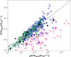 |
Fig. 5. Star formation rate (SFR) estimate from FIR luminosity vs. radio pseudo-SFR for all sources radio-detected and with IRAS 60 μm data (black diamonds). Star-forming galaxies (green circles), RQ quasars (blue circles) and RL quasars (pink circles) are from Bonzini et al. (2015), with their pSFRradio converted using Eq. 22 of Molnár et al. (2021). The dashed line is the 1:1 ratio line of equal SFR. |
3.5. Classification of the dominating radio mechanism
The radio emission from sources in our sample may arise from a combination of SF, AGN-driven winds or outflows, relativistic jets, and/or accretion disc coronal emission (Chen et al. 2022). For each source, we identified the dominating mechanisms based on the combination of several indicators, as detailed in Table 2. For reference, we also show the calculated Kellermann parameter, Rk, for each source, although it was not used in the classification. Figure 6 shows the classification scheme adopted in this work, with details given below.
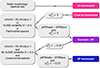 |
Fig. 6. Summary of the classification scheme used to identify the dominant radio emission mechanism for each sources in our sample, based on the combination of indicators compiled in Table 2. |
Dominant radio mechanism indicators and overall source classification.
We first consider the radio luminosity, which for starbursts typically does not exceed νLν, int = 1E+40 erg s−1 (Sargsyan & Weedman 2009). We adopt the limit from Zamfir et al. (2008), log L1.4 GHz = 31.6 erg s−1 Hz−1. This indicates that the radio emission from at least four of our 18 sources must have an AGN-related component (core or jet). We note three sources of our sample with significant radio variability at 3 GHz (V > 0.1), namely J12091+5611, J12562+5652, and J15455+4846, which indicates a core- or jet-related origin. We also consider the shape of the radio spectra obtained in Section 3.3. Star formation (SF) produces a synchrotron spectrum with α = −0.8 ± 0.4, no significant curvature from 1 − 10 GHz, and a spectral turnover at a few hundred megahertz. Radio emission from AGN jets has steeper spectral slopes with increasing frequencies, indicating the aging of the relativistic electron population due to inverse-Compton, synchrotron, ionization, or bremsstrahlung energy losses. A core-dominated jet or accretion disk corona produces optically thick synchrotron emission, characterized by a flat or inverted spectrum. Among the 16 detected sources in at least three bands, two show flat or inverted spectra between 144 MHz (or 1.5 GHz) and 10 GHz, namely J12562+5652 and J14258+3946, with fitted spectral indices of 0.5 ± 0.3 and 1.0 ± 0.2, respectively. Both are RL sources. J12562+5652 shows some extended emission, particularly at 144 MHz; however, because it is the brightest source in the sample, the limited dynamical range achievable with the short VLA exposure may have prevented the detection of faint extended emission at higher frequencies (note the unusually high rms values reported in Table B.1 for this target). This effect explains why the flux density measured at 144 MHz appears to be well above the fit spectral slope. J14258+3946 is the most luminous source in our sample and also has the highest  = 0.16.
The nonsimultaneity of the observations (LOFAR and VLASS) and the mismatch in resolution between frequencies prevent a clear differentiation between SF and jet origin for the remaining sources with linear or curved spectrum.
J17014+5149 is the only source in which we resolve two symmetric radio jets. The two distinct point-like sources resolved at higher frequencies exhibit identical α5 − 10 = −1.0 ± 0.1 (within the uncertainties). It also has the second highest radio luminosity of the sample. Based on this morphology, we classify J17014+5149 as jet-dominated. For the remaining sources, their morphologies, or mere presence or absence of extended emission, do not allow us to further constrain the classification.
Although correlation is not causation, we consider that the ten sources with pSFRradio ≃ SFR60 μm likely have radio emission originating from SF (see Fig. 5). None of these sources lie below the correlation, indicating that the entire detected radio emission can originate from SF. In addition to this criterion, we consider the two-point spectral index between radio and mid-IR (see Figure 4). We separated sources with  , typical of star-forming IR galaxies, from those with
  , which are more typical of core or jets. For the remaining sources, the radio emission likely originates from a combination of AGN and SF. Only one source, J12075+1506, for which IR data are not available, cannot be classified following the scheme in Figure 6. However, since it has log L1.4 GHz > 31.6 erg s−1 Hz−1 and
  , we interpret the origin of its emission as a combination of AGN and SF.
Overall, we find that seven of our 18 targets likely have radio emission dominantly from SF, while six show a combination of SF and AGN-related mechanisms. Only three sources (all RL) indicate a core- or jet-only AGN origin for the detected radio emission. Among the eight RL sources, we classify one as SF-dominated and four as exhibiting a combination of SF and AGN-related mechanisms.
3.6. Bremsstrahlung radio emission
Free-free (bremsstrahlung) emission arises from hot, ionized gas. The mechanism itself operates independently of bulk motion, while a BLR or a NLR wind could contribute to or enhance such emission, particularly by providing a more extended or structured ionized medium. Most super-Eddington sources in our sample exhibit evidence of [O III]λλ4959,5007 outflows (see the multicomponent, nonlinear analysis of the [O III]λλ4959,5007 line and the wind parameter estimates in Appendix C), which in some cases are powerful enough to dominate the line emission. For sources with high Eddington ratios, free-free emission associated with a wind could plausibly contribute to their radio output (Blundell & Kuncic 2007; Chen et al. 2024).
As discussed in Sect. 3.3, the radio spectral indices of our sample are generally inconsistent with solely optically thin or thick bremsstrahlung emission (Baskin & Laor 2021) or with emission from a corona. The energetics of the [O III]λ5007 outflows also disfavor bremsstrahlung emission as the origin of the radio power.
The mass of the gas emitting the [O III]λ5007 lines can be computed using a conversion between line luminosity and gas mass (Cano-Díaz et al. 2012; Carniani et al. 2015; Marziani et al. 2016b, 2017; Fiore et al. 2017):
![Mathematical equation: $$ \begin{aligned} M_{\rm [OIII]} \sim 1\cdot 10^6 L_{44}\left(\frac{Z}{5\,Z_\odot }\right)^{-1} n_{4}^{-1}\,\mathrm{M} _\odot , \end{aligned} $$](/articles/aa/full_html/2026/03/aa57025-25/aa57025-25-eq27.gif) (9)
(9)
where the line luminosity is expressed in units of 1044 erg s−1, the metallicity is scaled to five times solar, and the density is normalized to 104 cm−3. Given the free-free emissivity jff (Rybicki & Lightman 1979), the radio power expected from the emitting gas is
![Mathematical equation: $$ \begin{aligned} P_{\nu ,\mathrm{[OIII]} } \sim \frac{M_{\rm [OIII]}}{n \mu m_{\rm p}} j_{\rm ff}&\sim&2.9 \cdot 10^{29} \bar{g}_{10} \, T_{\rm e,10\,000}^{-1/2} Z_{5} ^{-1} \cdot \\&n_{\rm 4} L_{\mathrm{[OIII]} ,44}\,\mathrm {erg\,s}^{-1}\,\mathrm{Hz}^{-1} \nonumber , \end{aligned} $$](/articles/aa/full_html/2026/03/aa57025-25/aa57025-25-eq28.gif) (10)
(10)
where  is the average Gaunt factor normalized to ten (Van Hoof et al. 2014, 2015; Chluba et al. 2020). The typical density of the spatially resolved NLR is n ≳ 103 cm−3 (Singha et al. 2022, cf. Kakkad et al. 2018), while the innermost part of the NLR in NGC 5548 has an estimated density of n ∼ 105 cm−3 (Peterson et al. 2013). We therefore scaled the equation for the radio-power to n ∼ 104 cm−3. With this density, the observed median [O III]λ5007 luminosity of ∼1042 erg s−1 (Appendix C) is insufficient to explain the observed radio power, especially if L1.4 GHz ≳ 1031 erg s−1 Hz−1. In the case of a compact NLR (Zamanov et al. 2002), however, a higher density of ∼105 cm−3 in the [O III]λ5007 emitting region could account for powers comparable to L1.4 GHz ∼ 1029 erg s−1 Hz−1.
3.7. Correlation analysis
3.7.1. Accretion parameters versus radio spectral indices
Laor et al. (2019) compared the radio spectral index of a sample of 25 RQ Palomar–Green (PG) quasars with their Eddington ratios, the FWHM of the Hβ line, the flux ratio RFeII, and MBH. They found that RQ and RL quasars display different trends. For the RQ quasars, the radio spectral indices correlate with both the FWHM of the Hβ line and the Eddington ratio. High Eddington ratio sources have steeper radio spectrum, indicative of an extended optically thin synchrotron source, such as a weak jet or wind component. In contrast, lower Eddington ratio sources have flatter radio spectra, indicative of a compact, optically thick synchrotron source, such as a compact core, a weak jet base, or an accretion disk corona. Radio-loud (RL) quasars do not show such a correlation, but their radio spectral indices correlate with MBH: most quasars with MBH > 109 M⊙ have steeper spectral indices (< − 0.5), dominated by extended lobe emission, whereas MBH < 109 M⊙ quasars have spectral indices > − 0.5, and their radio emission is unresolved.
We compare these results with our sample in Fig. 7. The distribution of our sources mainly overlaps that of the RQ quasars from Laor et al. (2019). Most of the xA data points (those classified as SF-dominated or having a combination of core and jet emission plus SF, all with α5 − 10 ≲ –0.5) are consistent with the high L/LEdd branch of Laor et al. (2019). One source in our sample (J12562+5652 ≡ Mark 231) is notable for its inverted spectrum (α5 − 10 > 0), and may correspond more closely to the RL regime of Laor et al. (2019). An important difference is that two core-jet dominated objects show RFeII > 1, while all RL sources of Laor et al. (2019) show RFeII ≲ 0.5, and these core-jet dominated sources in our sample have Eddington ratios close to unity.
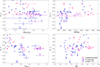 |
Fig. 7. Spectral index α5 − 10 vs. the Eddington ratio, the FWHM of the Hβ line (in km/s), the flux ratio RFeII, and MBH. Markers are colored according to the dominant mechanism responsible for the detected radio emission (Table 2). Blue and pink filled circles indicate RQ and RL quasars, respectively, from Laor et al. (2019). |
3.7.2. Correlation of radio, IR, and optical data
The data enable a correlation analysis between radio, IR, and optical spectral properties. Fig. C.2 presents the results for most of the parameters measured in this work (from Tables B.4, C.1, C.2 and C.4, or computed as explained in the previous sections). Apart from some predictable correlations (e.g., MBH and L/LEdd with luminosity), correlations between RFeII and L/LEdd have been observed or predicted in several previous studies (Marziani et al. 2001; Sun & Shen 2015; Du et al. 2016; Marziani et al. 2025, and references therein). This correlation is relatively weak, as nearly all sources in the sample are strong Fe II-emitters, implying low equivalent widths despite broad [O III]λλ4959,5007 and blueward asymmetries in both Hβ and [O III]λ5007. The anti-correlation between [O III]λ5007 blue peak shift and its FWHM is typical of compact, wind-dominated narrow-line regions (NLR, Zamanov et al. 2002; Marziani et al. 2016b; Coatman et al. 2016; Deconto-Machado et al. 2023). A notable result is the absence of a strong correlation (rP ≲ 0.3) between radio power and [O III]λ5007 and Hβ mass outflow rates Ṁ Hβ.
3.7.3. Principal component analysis
The Eigenvector 1 (E1) of quasars has been retrieved in samples where the RFeII range is ≈0 − 2 (Boroson & Green 1992). In the present sample, the median RFeII is approximately 1.19, with the first quartile at RFeII ≈ 1.09, and only one object (J10255+5140) exhibiting RFeII ≈0.8. Given the correlation between RFeII and L/LEdd (Du et al. 2016; Panda et al. 2019) and the relatively small variation of L/LEdd for RFeII ≳ 1 (Marziani et al. 2025), we do not expect to detect E1 in our sample. The principle component analysis (PCA) applied to our sample reveals only one eigenvector with a clear physical meaning. Fig. 8 presents the projection of the targets and the loads of each vector along principal component 1 (PC1). The PC1 carries ≈34% of the sample variance, slightly more than the original E1; however, it is associated with luminosity trends, i.e., the original eigenvector 2 of Boroson & Green (1992). The left panel of Fig. 8 shows our sources aligned along the PC1: the least and most luminous occupy opposite ends of the vector.
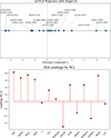 |
Fig. 8. Results of the PCA analysis. Top: 1D projection of sources along the PC1. Bottom: Vector loading along the PC1. |
4. Discussion
4.1. Significance of the high RFeII and jetted super-Eddington candidates
In our sample, three sources (J12091+5611, J14258+3946, and J17014+5149; all RL) have radio emission predominantly produced by a core or jetted AGN. Fig. 1 shows that the prevalence of radio-detected and genuinely jetted sources from an optically selected sample depends on the location along the MS. A rigorous assessment of the incidence of jetted sources requires homogeneous datasets and well-defined parent samples, which are not currently available. As a pragmatic proxy, one may consider NLSy1s, although only a minority satisfy the condition RFeII ≳ 1. Although the most powerful radio sources belong to spectral type B, a population of lower-power, yet jetted, objects appears among NLSy1s (Komossa et al. 2006; Foschini et al. 2015; Foschini 2020; Ojha et al. 2024, 2026). About 7% of NLSy1s are RL, with an even smaller fraction (∼2.5%) reaching very high radio loudness (RK > 100) (Orienti et al. 2015). Far fewer sources appear in the γ-ray domain: ≲30 are currently known (Foschini 2020; Foschini et al. 2022; Dalla Barba et al. 2026). Moreover, objects with reliable measurements (i.e., high S/N optical spectra) that simultaneously satisfy RFeII ≳ 1 and show clear evidence of jets, as indicated by a high radio-loudness parameter log RK ≳ 1.8 (Zamfir et al. 2008), are extremely rare. A search in the recent catalog by Paliya et al. (2023) returns only a handful of candidates among ∼28,000 NLSy1s. Among these, only a few of the γ-ray emitters would be classified as xA. Garnica et al. (2025) report a few additional jetted candidates in their sample, defined by RFeII ≳ 0.9. Furthermore, some observational studies report compact or jet-like radio emission in high-Eddington systems among X-ray quasars detected by eROSITA (e.g., Khorunzhev et al. 2021; Wolf et al. 2021; Obuchi et al. 2025).
Super-Eddington accretors with relativistic ejections imply that thick, wind-dominated accretion flows can still generate and sustain magnetically driven, collimated jets. Such coexistence is expected in a magnetically arrested disk (MAD) regime because super-Eddington disks are geometrically thick and tend to create a low-density polar funnel while simultaneously launching a wide-angle wind from the disk surface (McKinney et al. 2015; Yang et al. 2023). The main threat to a highly relativistic jet is mass loading (baryons and radiation) in or near the funnel, which can reduce jet magnetization and terminal Lorentz factor (McKinney et al. 2015). The identification of jetted super-Eddington candidates is therefore of particular importance for understanding the accretion process, and the sources identified in the present work should be considered for dedicated studies.
4.2. High-rate accretion and star formation
The analysis presented in the previous sections indicates that SF contributes to the radio emission of many sources in our sample. Indeed, most sources exhibit radio spectral indices consistent with either SF or optically thin jet emission. However, correlations between IR and radio properties reveal a high prevalence of composite-origin or even SF-dominated systems, highlighting the importance of multiwavelength analysis using several indicators.
We selected our sample based on the optical selection criterion RFeII ≳1, which isolates spectral types A3 and A4 within the 4DE1 formalism (Sulentic et al. 2000b). This selection is independent of radio properties, thereby avoiding any explicit bias toward RL or RQ AGN. Sources in the A3 and A4 bins are generally interpreted as radiating at high Eddington ratios, a key driver of E1. They are characterized by strong Fe II emission, narrow Balmer lines, and weak but semi-broad C IVλ1549, all hallmarks of high accretion states. This reflects the coexistence of a virialized low-ionization BLR coexisting with an outflowing, mildly ionized system involving both broad and narrow lines (Collin-Souffrin & Lasota 1988; Elvis 2000; Marziani et al. 2010). Our high-Eddington-ratio sample reveals a high prevalence of composite or SF-dominated radio systems. Our results confirm previous SDSS-based statistical findings: a significant fraction of high-RFeII sources exhibit either composite radio emission or emission dominated by SF (Bonzini et al. 2015; Ganci et al. 2019). Consistent results were also found in analyses of NLSy1 samples (Sani et al. 2010; Caccianiga et al. 2015), which contain a large fraction of highly accreting sources (although not all NLSy1s are highly accreting sources; see Marziani et al. 2018). The evidence indicates that in the high-Eddington-ratio regime, the prevalence of powerful relativistic jets decreases, whereas other forms of radio emission–such as compact or diffuse low-power radio structures associated with winds, disk instabilities, or star-forming activity–become more common. The relative paucity of high-radio-power sources in low MBH AGNs may support a mechanism in which the radio power scales with MBH, such as energy extraction from a spinning black hole threaded by magnetic fields (Blandford & Znajek 1977; Foschini 2014; Foschini et al. 2024).
The E1 main sequence, even at low redshifts, permits an evolutionary interpretation (Fraix-Burnet et al. 2017): from highly accreting low mass AGNs to evolved, massive black holes accreting at rates just sufficient to sustain radiatively efficient accretion (Giustini & Proga 2019). Figure 7 of Yue et al. (2025) shows cumulative MBH distributions for AGN whose low-frequency radio is AGN- and SF-dominated, presented across luminosity and redshift grids. A key finding is the consistent offset: AGN-dominated quasars exhibit systematically higher black hole masses than SF-dominated quasars across all bins. For a sample with high RFeII ≳1, which maps to spectral types A3 and A4 and high Eddington ratios, the results of Yue et al. (2025) are particularly informative: sources with lower MBH are expected to have relatively higher L/LEdd at fixed luminosity due to the inverse relation between L/LEdd and MBH for a given bolometric output. The star-formation-dominated quasars, which likely correspond to high-L/LEdd systems in our sample, tend to be less massive than their jetted counterparts. This behavior extends consistently from low redshift to beyond the cosmic noon, suggesting a common pattern in quasar evolution and black hole growth, where SF, possibly due to merger-induced gas enhancement near the active nucleus, coexists in the early phases of black hole growth. As quasars evolve from xA to extreme population B, black hole masses increase, and the circumnuclear stellar system also evolves, with some stars following accretion-modified stellar evolution patterns (e.g., Wang et al. 2010, 2009; Cantiello et al. 2021; Fabj & Samsing 2024). Ultimately, the most massive black holes are expected to be surrounded by a stellar graveyard (Marziani et al. 2025).
5. Conclusions
We present new VLA observations at L, C and X bands for a sample of 18 quasars accreting at very high rates, complemented with LoTSS and VLASS observations. We identified the dominating mechanism behind the detected radio emission of these sources based on a combination of several indicators: radio variability, luminosity, morphology, radio spectral properties, and radio-to-mid IR flux ratio. Seven of our 18 targets likely have radio emission dominantly from SF, six show a combination of SF and AGN-related mechanisms, and only three sources appear to have radio emission originating solely from a core or jetted AGN. These results are consistent with previous studies and suggest that, in the high–Eddington-ratio regime, radio emission is more commonly associated with lower-power structures related to SF than with relativistic jets. This fits the common quasar evolutionary pattern, in which SF coexists during early black hole growth phases. A PCA analysis confirms the tendency toward homogeneous properties of our samples – consistent with a common spectral type – with the first eigenvector associated with luminosity-dependent effects.
We complemented this analysis with a multicomponent nonlinear decomposition of Hβ and [O III]λλ4959,5007 lines, from which we derived estimates of accretion and wind parameters. Although these sources are candidate super-Eddington quasars, their NLR and BLR winds produce only modest feedback, particularly at low-luminosity. We estimated the bremsstrahlung emission associated with the conditions required for the formation of the [O III]λλ4959,5007 lines under photoionization from the active nucleus, but find no clear evidence of its contribution to the total radio power in our sample.
With its unparalleled sensitivity and angular resolution, the upcoming Square Kilometre Array Observatory will enable similar studies and allow us to probe the evolution of these objects at much earlier times (e.g., Latif et al. 2024).
Acknowledgments
MLGM and LVM acknowledge financial support from the grant CEX2021-001131-S funded by MICIU/AEI/10.13039/501100011033, from the grant PID2021-123930OB-C21 funded by MICIU/AEI/10.13039/501100011033 and by ERDF/EU. MLGM acknowledges financial support from NSERC via the Discovery grant program and the Canada Research Chair program. AdO and PM acknowledge financial support from the Spanish MCIU through project PID2022-140871NB-C21 by “ERDF A way of making Europe”, and from the Severo Ochoa grant CEX2021-515001131-S funded by MCIN/AEI/10.13039/501100011033. LOFAR is the Low Frequency Array designed and constructed by ASTRON. It has observing, data processing, and data storage facilities in several countries, which are owned by various parties (each with their own funding sources), and which are collectively operated by the ILT foundation under a joint scientific policy. The ILT resources have benefited from the following recent major funding sources: CNRS-INSU, Observatoire de Paris and Université d’Orléans, France; BMBF, MIWF-NRW, MPG, Germany; Science Foundation Ireland (SFI), Department of Business, Enterprise and Innovation (DBEI), Ireland; NWO, The Netherlands; The Science and Technology Facilities Council, UK; Ministry of Science and Higher Education, Poland; The Istituto Nazionale di Astrofisica (INAF), Italy. This research has made use of the NASA/IPAC Extragalactic Database (NED), which is operated by the Jet Propulsion Laboratory, California Institute of Technology, under contract with the National Aeronautics and Space Administration. This research has made use of the NASA/IPAC Infrared Science Archive, which is funded by the National Aeronautics and Space Administration and operated by the California Institute of Technology.
References
- Aller, M. F., Aller, H. D., & Hughes, P. A. 1992, ApJ, 399, 16 [NASA ADS] [CrossRef] [Google Scholar]
- Azzalini, A. 1985, Scand. J. Stat., 12, 171 [Google Scholar]
- Baskin, A., & Laor, A. 2021, MNRAS, 508, 680 [NASA ADS] [CrossRef] [Google Scholar]
- Belladitta, S., Moretti, A., Caccianiga, A., et al. 2019, A&A, 629, A68 [NASA ADS] [CrossRef] [EDP Sciences] [Google Scholar]
- Bentz, M. C., Peterson, B. M., Netzer, H., Pogge, R. W., & Vestergaard, M. 2009, ApJ, 697, 160 [Google Scholar]
- Berton, M., & Järvelä, E. 2021, Universe, 7, 188 [NASA ADS] [CrossRef] [Google Scholar]
- Berton, M., Foschini, L., Ciroi, S., et al. 2016, A&A, 591, A88 [NASA ADS] [CrossRef] [EDP Sciences] [Google Scholar]
- Berton, M., Congiu, E., Järvelä, E., et al. 2018, A&A, 614, A87 [NASA ADS] [CrossRef] [EDP Sciences] [Google Scholar]
- Berton, M., Järvelä, E., Crepaldi, L., et al. 2020, A&A, 636, A64 [NASA ADS] [CrossRef] [EDP Sciences] [Google Scholar]
- Bischetti, M., Piconcelli, E., Vietri, G., et al. 2017, A&A, 598, A122 [NASA ADS] [CrossRef] [EDP Sciences] [Google Scholar]
- Blandford, R. D., & Znajek, R. L. 1977, MNRAS, 179, 433 [NASA ADS] [CrossRef] [Google Scholar]
- Blundell, K. M., & Kuncic, Z. 2007, ApJ, 668, L103 [NASA ADS] [CrossRef] [Google Scholar]
- Bonzini, M., Mainieri, V., Padovani, P., et al. 2015, MNRAS, 453, 1079 [Google Scholar]
- Boroson, T. A., & Green, R. F. 1992, ApJS, 80, 109 [Google Scholar]
- Caccianiga, A., Antón, S., Ballo, L., et al. 2015, MNRAS, 451, 1795 [NASA ADS] [CrossRef] [Google Scholar]
- Cano-Díaz, M., Maiolino, R., Marconi, A., et al. 2012, A&A, 537, L8 [NASA ADS] [CrossRef] [EDP Sciences] [Google Scholar]
- Cantiello, M., Jermyn, A. S., & Lin, D. N. C. 2021, ApJ, 910, 94 [NASA ADS] [CrossRef] [Google Scholar]
- Carniani, S., Marconi, A., Maiolino, R., et al. 2015, A&A, 580, A102 [NASA ADS] [CrossRef] [EDP Sciences] [Google Scholar]
- Casa, T., Bean, B., Bhatnagar, S., et al. 2022, PASP, 134, 114501 [NASA ADS] [CrossRef] [Google Scholar]
- Chen, S., Stevens, J. B., Edwards, P. G., et al. 2022, MNRAS, 512, 471 [Google Scholar]
- Chen, S., Laor, A., Behar, E., et al. 2024, ApJ, 975, 35 [Google Scholar]
- Chluba, J., Ravenni, A., & Bolliet, B. 2020, MNRAS, 492, 177 [Google Scholar]
- Coatman, L., Hewett, P. C., Banerji, M., & Richards, G. T. 2016, MNRAS, 461, 647 [NASA ADS] [CrossRef] [Google Scholar]
- Collin-Souffrin, S., & Lasota, J.-P. 1988, PASP, 100, 1041 [NASA ADS] [CrossRef] [Google Scholar]
- Condon, J. J. 1989, ApJ, 338, 13 [NASA ADS] [CrossRef] [Google Scholar]
- Condon, J. J., Huang, Z.-P., Yin, Q. F., & Thuan, T. X. 1991, ApJ, 378, 65 [NASA ADS] [CrossRef] [Google Scholar]
- Cornwell, T. J. 2008, IEEE J. Sel. Topics Signal Process., 2, 793 [Google Scholar]
- Cornwell, T. J., Golap, K., & Bhatnagar, S. 2008, IEEE J. Sel. Topics Signal Process., 2, 647 [Google Scholar]
- Cracco, V., Ciroi, S., Berton, M., et al. 2016, MNRAS, 462, 1256 [NASA ADS] [CrossRef] [Google Scholar]
- Crepaldi, L., Berton, M., Dalla Barba, B., et al. 2025, A&A, 696, A74 [NASA ADS] [CrossRef] [EDP Sciences] [Google Scholar]
- Cresci, G., Mainieri, V., Brusa, M., et al. 2015, ApJ, 799, 82 [Google Scholar]
- Czerny, B., Beaton, R., Bejger, M., et al. 2018, Space Sci. Rev., 214, 32 [Google Scholar]
- Dalla Barba, B., Foschini, L., Berton, M., et al. 2026, A&A, 705, A122 [NASA ADS] [CrossRef] [EDP Sciences] [Google Scholar]
- Decarli, R., Walter, F., Venemans, B. P., et al. 2017, Nature, 545, 457 [Google Scholar]
- Deconto-Machado, A., Del Olmo Orozco, A., Marziani, P., Perea, J., & Stirpe, G. M. 2023, A&A, 669, A83 [NASA ADS] [CrossRef] [EDP Sciences] [Google Scholar]
- Deconto-Machado, A., Del Olmo, A., & Marziani, P. 2024, A&A, 691, A15 [NASA ADS] [CrossRef] [EDP Sciences] [Google Scholar]
- Di Matteo, T., Springel, V., & Hernquist, L. 2005, Nat, 433, 604 [Google Scholar]
- Diamond-Stanic, A. M., & Rieke, G. H. 2012, ApJ, 746, 168 [Google Scholar]
- D’Onofrio, M., Marziani, P., Chiosi, C., & Negrete, C. A. 2024, Universe, 10, 254 [CrossRef] [Google Scholar]
- Du, P., & Wang, J.-M. 2019, ApJ, 886, 42 [NASA ADS] [CrossRef] [Google Scholar]
- Du, P., Wang, J.-M., Hu, C., et al. 2016, ApJ, 818, L14 [NASA ADS] [CrossRef] [Google Scholar]
- Elvis, M. 2000, ApJ, 545, 63 [NASA ADS] [CrossRef] [Google Scholar]
- Fabj, G., & Samsing, J. 2024, MNRAS, 535, 3630 [Google Scholar]
- Ferland, G. J., Done, C., Jin, C., Landt, H., & Ward, M. J. 2020, MNRAS, 494, 5917 [Google Scholar]
- Fiore, F., Feruglio, C., Shankar, F., et al. 2017, A&A, 601, A143 [NASA ADS] [CrossRef] [EDP Sciences] [Google Scholar]
- Foschini, L. 2014, Int. J. Mod. Phys. Conf. Ser., 28, 1460188 [NASA ADS] [CrossRef] [Google Scholar]
- Foschini, L. 2020, Universe, 6, 136 [NASA ADS] [CrossRef] [Google Scholar]
- Foschini, L., Berton, M., Caccianiga, A., et al. 2015, A&A, 575, A13 [NASA ADS] [CrossRef] [EDP Sciences] [Google Scholar]
- Foschini, L., Lister, M. L., Andernach, H., et al. 2022, Universe, 8, 587 [NASA ADS] [CrossRef] [Google Scholar]
- Foschini, L., Dalla Barba, B., Tornikoski, M., et al. 2024, Universe, 10, 156 [Google Scholar]
- Fraix-Burnet, D., D’Onofrio, M., & Marziani, P. 2017, Front. Astron. Space Sci., 4 [Google Scholar]
- Fuller, L., Lopez-Rodriguez, E., Packham, C., et al. 2019, MNRAS, 483, 3404 [NASA ADS] [CrossRef] [Google Scholar]
- Ganci, V., Marziani, P., D’Onofrio, M., et al. 2019, A&A, 630, A110 [NASA ADS] [CrossRef] [EDP Sciences] [Google Scholar]
- Garnica, K., Dultzin, D., Marziani, P., & Panda, S. 2025, The spectral energy distribution of extreme population A quasars [Google Scholar]
- Giustini, M., & Proga, D. 2019, A&A, 630, A94 [NASA ADS] [CrossRef] [EDP Sciences] [Google Scholar]
- Greene, J. E., & Ho, L. C. 2005, ApJ, 630, 122 [NASA ADS] [CrossRef] [Google Scholar]
- Halpern, J. P., & Oke, J. B. 1987, ApJ, 312, 91 [NASA ADS] [CrossRef] [Google Scholar]
- Harrison, C. M., Alexander, D. M., Mullaney, J. R., & Swinbank, A. M. 2014, MNRAS, 441, 3306 [Google Scholar]
- Heinz, S., & Sunyaev, R. A. 2003, MNRAS, 343, L59 [Google Scholar]
- Helou, G., Soifer, B. T., & Rowan-Robinson, M. 1985, ApJ, 298, L7 [Google Scholar]
- Ishibashi, W., & Fabian, A. C. 2012, MNRAS, 427, 2998 [NASA ADS] [CrossRef] [Google Scholar]
- Jarrett, T. H., Cohen, M., Masci, F., et al. 2011, ApJ, 735, 112 [Google Scholar]
- Järvelä, E., Berton, M., & Crepaldi, L. 2021, Front. Astron. Space Sci., 8 [Google Scholar]
- Järvelä, E., Dahale, R., Crepaldi, L., et al. 2022, A&A, 658, A12 [NASA ADS] [CrossRef] [EDP Sciences] [Google Scholar]
- Jarvis, M. J., & McLure, R. J. 2006, MNRAS, 369, 182 [CrossRef] [Google Scholar]
- Kakkad, D., Groves, B., Dopita, M., et al. 2018, A&A, 618, A6 [NASA ADS] [CrossRef] [EDP Sciences] [Google Scholar]
- Kakkad, D., Mainieri, V., Vietri, G., et al. 2020, A&A, 642, A147 [NASA ADS] [CrossRef] [EDP Sciences] [Google Scholar]
- Kakkad, D., Sani, E., Rojas, A. F., et al. 2022, MNRAS, 511, 2105 [NASA ADS] [CrossRef] [Google Scholar]
- Kellermann, K. I., Sramek, R., Schmidt, M., Shaffer, D. B., & Green, R. 1989, AJ, 98, 1195 [Google Scholar]
- Kennicutt, R. C. 1998, ARA&A, 36, 189 [NASA ADS] [CrossRef] [Google Scholar]
- Kessler, M. F., Steinz, J. A., Anderegg, M. E., et al. 1996, A&A, 315, L27 [NASA ADS] [Google Scholar]
- Khorunzhev, G. A., Meshcheryakov, A. V., Medvedev, P. S., et al. 2021, Astron. Lett., 47, 123 [NASA ADS] [CrossRef] [Google Scholar]
- King, A., & Muldrew, S. I. 2016, MNRAS, 455, 1211 [CrossRef] [Google Scholar]
- King, A., & Pounds, K. 2015, ARA&A, 53, 115 [NASA ADS] [CrossRef] [Google Scholar]
- Komossa, S., Voges, W., Xu, D., et al. 2006, AJ, 132, 531 [NASA ADS] [CrossRef] [Google Scholar]
- Kunert-Bajraszewska, M., Krauze, A., Kimball, A. E., et al. 2025, ApJS, 277, 50 [Google Scholar]
- Lacy, M., Baum, S. A., Chandler, C. J., et al. 2020, PASP, 132, 035001 [Google Scholar]
- Laha, S., Reynolds, C. S., Reeves, J., et al. 2020, Nat. Astron., 5, 13 [Google Scholar]
- Lähteenmäki, A., Järvelä, E., Ramakrishnan, V., et al. 2018, A&A, 614, L1 [NASA ADS] [CrossRef] [EDP Sciences] [Google Scholar]
- Laor, A., Baldi, R. D., & Behar, E. 2019, MNRAS, 482, 5513 [NASA ADS] [CrossRef] [Google Scholar]
- Latif, M. A., Whalen, D. J., & Mezcua, M. 2024, MNRAS, 527, L37 [Google Scholar]
- Leighly, K. M., & Moore, J. R. 2004, ApJ, 611, 107 [Google Scholar]
- Liska, M. T. P., Musoke, G., Tchekhovskoy, A., Porth, O., & Beloborodov, A. M. 2022, ApJ, 935, L1 [NASA ADS] [CrossRef] [Google Scholar]
- Mancuso, C., Lapi, A., Prandoni, I., et al. 2017, ApJ, 842, 95 [Google Scholar]
- Martínez-Aldama, M. L., Del Olmo, A., Marziani, P., et al. 2018, A&A, 618, A179 [NASA ADS] [CrossRef] [EDP Sciences] [Google Scholar]
- Martínez-Aldama, M. L., Zajacek, M., Czerny, B., & Panda, S. 2020, ApJ, 903, 86 [CrossRef] [Google Scholar]
- Marziani, P., & Sulentic, J. W. 2014, MNRAS, 442, 1211 [NASA ADS] [CrossRef] [Google Scholar]
- Marziani, P., Sulentic, J. W., Zwitter, T., Dultzin-Hacyan, D., & Calvani, M. 2001, ApJ, 558, 553 [NASA ADS] [CrossRef] [Google Scholar]
- Marziani, P., Sulentic, J. W., Zamanov, R., et al. 2003, ApJS, 145, 199 [NASA ADS] [CrossRef] [Google Scholar]
- Marziani, P., Sulentic, J. W., Negrete, C. A., et al. 2010, MNRAS, 409, 1033 [Google Scholar]
- Marziani, P., Sulentic, J. W., Plauchu-Frayn, I., & Olmo, A. D. 2013, A&A, 555, A89 [NASA ADS] [CrossRef] [EDP Sciences] [Google Scholar]
- Marziani, P., Martínez Carballo, M. A., Sulentic, J. W., et al. 2016a, Ap&SS, 361, 29 [NASA ADS] [CrossRef] [Google Scholar]
- Marziani, P., Sulentic, J. W., Stirpe, G. M., et al. 2016b, Ap&SS, 361, 3 [NASA ADS] [CrossRef] [Google Scholar]
- Marziani, P., Negrete, C. A., Dultzin, D., et al. 2017, Front. Astron. Space Sci., 4, 16 [NASA ADS] [CrossRef] [Google Scholar]
- Marziani, P., Dultzin, D., Sulentic, J. W., et al. 2018, Front. Astron. Space Sci., 5, 6 [CrossRef] [Google Scholar]
- Marziani, P., Berton, M., Panda, S., & Bon, E. 2021, Universe, 7, 484 [NASA ADS] [CrossRef] [Google Scholar]
- Marziani, P., Olmo, A. D., Negrete, C. A., et al. 2022, ApJS, 261, 30 [NASA ADS] [CrossRef] [Google Scholar]
- Marziani, P., Garnica Luna, K., Floris, A., et al. 2025, Universe, 11, 69 [Google Scholar]
- Mathur, S. 2000, MNRAS, 314, L17 [NASA ADS] [CrossRef] [Google Scholar]
- McKinney, J. C., Dai, L., & Avara, M. J. 2015, MNRAS, 454, L6 [NASA ADS] [CrossRef] [Google Scholar]
- McKinney, J. C., Chluba, J., Wielgus, M., Narayan, R., & Sadowski, A. 2017, MNRAS, 467, 2241 [Google Scholar]
- Mejía-Restrepo, J. E., Lira, P., Netzer, H., Trakhtenbrot, B., & Capellupo, D. M. 2018, Nat. Astron., 2, 63 [CrossRef] [Google Scholar]
- Mineshige, S., Kawaguchi, T., Takeuchi, M., & Hayashida, K. 2000, PASJ, 52, 499 [NASA ADS] [CrossRef] [Google Scholar]
- Molnár, D. C., Sargent, M. T., Leslie, S., et al. 2021, MNRAS, 504, 118 [CrossRef] [Google Scholar]
- Mor, R., & Netzer, H. 2012, MNRAS, 420, 526 [NASA ADS] [CrossRef] [Google Scholar]
- Murakami, H., Baba, H., Barthel, P., et al. 2007, PASJ, 59, S369 [CrossRef] [Google Scholar]
- Nardini, E., Lusso, E., Risaliti, G., et al. 2019, A&A, 632, A109 [NASA ADS] [CrossRef] [EDP Sciences] [Google Scholar]
- Negrete, C. A., Dultzin, D., Marziani, P., & Sulentic, J. W. 2012, ApJ, 757, 62 [NASA ADS] [CrossRef] [Google Scholar]
- Negrete, C. A., Dultzin, D., Marziani, P., et al. 2018, A&A, 620, A118 [NASA ADS] [CrossRef] [EDP Sciences] [Google Scholar]
- Netzer, H. 2013, The Physics and Evolution of Active Galactic Nuclei [Google Scholar]
- Netzer, H. 2019, MNRAS, 488, 5185 [NASA ADS] [CrossRef] [Google Scholar]
- Netzer, H., & Marziani, P. 2010, ApJ, 724, 318 [NASA ADS] [CrossRef] [Google Scholar]
- Netzer, H., Lani, C., Nordon, R., et al. 2016, ApJ, 819, 123 [Google Scholar]
- Neugebauer, G., Habing, H. J., van Duinen, R., et al. 1984, ApJ, 278, L1 [NASA ADS] [CrossRef] [Google Scholar]
- Obuchi, S., Ichikawa, K., Yamada, S., et al. 2025, Discovery of an X-ray Luminous Radio-Loud Quasar at z = 3.4: A Possible Transitional Super-Eddington Phase, version, Number, 1 [Google Scholar]
- O’Dea, C. 1998, PASP, 110, 493 [CrossRef] [Google Scholar]
- Ojha, V., Singh, V., Berton, M., & Järvelä, E. 2024, MNRAS, 529, L108 [Google Scholar]
- Ojha, V., Wu, X. B., Ho, L. C., et al. 2026, ArXiv e-prints [arXiv:2602.09171] [Google Scholar]
- Orienti, M., D’Ammando, F., Larsson, J., et al. 2015, MNRAS, 453, 4038 [Google Scholar]
- Osterbrock, D. E., & Ferland, G. J. 2006, Astrophysics of gaseous nebulae and active galactic nuclei [Google Scholar]
- Paliya, V. S., Stalin, C. S., Domínguez, A., & Saikia, D. J. 2023, MNRAS, 527, 7055 [NASA ADS] [CrossRef] [Google Scholar]
- Panda, S., Marziani, P., & Czerny, B. 2019, ApJ, 882, 79 [NASA ADS] [CrossRef] [Google Scholar]
- Peterson, B. M., Denney, K. D., De Rosa, G., et al. 2013, ApJ, 779, 109 [NASA ADS] [CrossRef] [Google Scholar]
- Reynolds, C., Punsly, B., Miniutti, G., O’Dea, C. P., & Hurley-Walker, N. 2017, ApJ, 836, 155 [Google Scholar]
- Rigopoulou, D., Lawrence, A., White, G. J., Rowan-Robinson, M., & Church, S. E. 1996, A&A, 305, 747 [NASA ADS] [Google Scholar]
- Runnoe, J. C., Brotherton, M. S., & Shang, Z. 2012, MNRAS, 422, 478 [Google Scholar]
- Rybicki, G. B., & Lightman, A. P. 1979, Radiative processes in astrophysics [Google Scholar]
- Sani, E., Lutz, D., Risaliti, G., et al. 2010, MNRAS, 403, 1246 [Google Scholar]
- Sargsyan, L. A., & Weedman, D. W. 2009, ApJ, 701, 1398 [NASA ADS] [CrossRef] [Google Scholar]
- Serjeant, S., & Hatziminaoglou, E. 2009, MNRAS, 397, 265 [NASA ADS] [CrossRef] [Google Scholar]
- Shapovalova, A. I., Popović, L. V., Burenkov, A. N., et al. 2012, ApJS, 202, 10 [NASA ADS] [CrossRef] [Google Scholar]
- Shen, Y. 2013, BASI, 41, 61 [Google Scholar]
- Shen, Y., Grier, C. J., Horne, K., et al. 2024, ApJS, 272, 26 [NASA ADS] [CrossRef] [Google Scholar]
- Shimwell, T. W., Hardcastle, M. J., Tasse, C., et al. 2022, A&A, 659, A1 [NASA ADS] [CrossRef] [EDP Sciences] [Google Scholar]
- Singha, M., Husemann, B., Urrutia, T., et al. 2022, A&A, 659, A123 [NASA ADS] [CrossRef] [EDP Sciences] [Google Scholar]
- Smith, J. D. T., Draine, B. T., Dale, D. A., et al. 2007, ApJ, 656, 770 [Google Scholar]
- Smolcic, V., Delvecchio, I., Zamorani, G., et al. 2017, A&A, 602, A2 [NASA ADS] [CrossRef] [EDP Sciences] [Google Scholar]
- Stickel, M., Lemke, D., Klaas, U., et al. 2000, A&A, 359, 865 [NASA ADS] [Google Scholar]
- Sulentic, J. W., Marziani, P., & Dultzin-Hacyan, D. 2000a, ARA&A, 38, 521 [Google Scholar]
- Sulentic, J. W., Zwitter, T., Marziani, P., & Dultzin-Hacyan, D. 2000b, ApJ, 536, L5 [Google Scholar]
- Sulentic, J. W., Marziani, P., Zamanov, R., et al. 2002, ApJ, 566, L71 [NASA ADS] [CrossRef] [Google Scholar]
- Sulentic, J. W., Dultzin-Hacyan, D., Bongardo, C., et al. 2006, RMxAA, 42, 23 [Google Scholar]
- Sun, J., & Shen, Y. 2015, ApJ, 804, L15 [Google Scholar]
- Temple, M. J., Ferland, G. J., Rankine, A. L., et al. 2020, MNRAS, 496, 2565 [NASA ADS] [CrossRef] [Google Scholar]
- Temple, M. J., Ferland, G. J., Rankine, A. L., Chatzikos, M., & Hewett, P. C. 2021, MNRAS, 505, 3247 [NASA ADS] [CrossRef] [Google Scholar]
- Van Hoof, P. A. M., Williams, R. J. R., Volk, K., et al. 2014, MNRAS, 444, 420 [NASA ADS] [CrossRef] [Google Scholar]
- Van Hoof, P. A. M., Ferland, G. J., Williams, R. J. R., et al. 2015, MNRAS, 449, 2112 [NASA ADS] [CrossRef] [Google Scholar]
- Veilleux, S., Meléndez, M., Tripp, T. M., Hamann, F., & Rupke, D. S. N. 2016, ApJ, 825, 42 [NASA ADS] [CrossRef] [Google Scholar]
- Vestergaard, M., & Peterson, B. M. 2006, ApJ, 641, 689 [Google Scholar]
- Vietri, G., Piconcelli, E., Bischetti, M., et al. 2018, A&A, 617, A81 [NASA ADS] [CrossRef] [EDP Sciences] [Google Scholar]
- Vietri, A., Järvelä, E., Berton, M., et al. 2022, A&A, 662, A20 [NASA ADS] [CrossRef] [EDP Sciences] [Google Scholar]
- Wang, J.-G., Dong, X.-B., Wang, T.-G., et al. 2009, ApJ, 707, 1334 [CrossRef] [Google Scholar]
- Wang, R., Carilli, C. L., Neri, R., et al. 2010, ApJ, 714, 699 [Google Scholar]
- Wang, J.-M., Qiu, J., Du, P., & Ho, L. C. 2014, ApJ, 797, 65 [NASA ADS] [CrossRef] [Google Scholar]
- Ward, S. R., Costa, T., Harrison, C. M., & Mainieri, V. 2024, AGN-driven outflows in clumpy media: multiphase structure and scaling relations, version Number: 2, 2 [Google Scholar]
- Wills, B. J., & Browne, I. W. A. 1986, ApJ, 302, 56 [NASA ADS] [CrossRef] [Google Scholar]
- Wolf, J., Nandra, K., Salvato, M., et al. 2021, A&A, 647, A5 [NASA ADS] [CrossRef] [EDP Sciences] [Google Scholar]
- Wolf, J., Nandra, K., Salvato, M., et al. 2023, A&A, 669, A127 [NASA ADS] [CrossRef] [EDP Sciences] [Google Scholar]
- Wright, E. L., Eisenhardt, P. R. M., Mainzer, A. K., et al. 2010, AJ, 140, 1868 [Google Scholar]
- Wu, Q. 2009, MNRAS, 398, 1905 [CrossRef] [Google Scholar]
- Xie, Y., & Ho, L. C. 2022, ApJ, 925, 218 [NASA ADS] [CrossRef] [Google Scholar]
- Yang, H., Yuan, F., Kwan, T., & Dai, L. 2023, MNRAS, 523, 208 [Google Scholar]
- Yue, B. H., Duncan, K. J., Best, P. N., et al. 2025, MNRAS, 537, 858 [Google Scholar]
- Yun, M. S., Reddy, N. A., & Condon, J. J. 2001, ApJ, 554, 803 [Google Scholar]
- Zamanov, R., Marziani, P., Sulentic, J. W., et al. 2002, ApJ, 576, L9 [NASA ADS] [CrossRef] [Google Scholar]
- Zamfir, S., Sulentic, J. W., & Marziani, P. 2008, MNRAS, 387, 856 [NASA ADS] [CrossRef] [Google Scholar]
- Zamfir, S., Sulentic, J. W., Marziani, P., & Dultzin, D. 2010, MNRAS, 403, 1759 [NASA ADS] [CrossRef] [Google Scholar]
- Zhang, K., Dong, X.-B., Wang, T.-G., & Gaskell, C. M. 2011, ApJ, 737, 71 [NASA ADS] [CrossRef] [Google Scholar]
The flux density scale calibration accuracy is based on the VLA Observational Status Summary 2020B.
Appendix A: Radio images, VLA observations setup, and variability
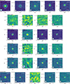 |
Fig. A.1. LOFAR (144 MHz) - when available - as well as our VLA L (1.5 GHz), C (5 GHz) and X (10 GHz) band images and VLASS (S-band, 3 GHz) of the 18 targets of the sample, each with a 5σ contour encompassing the main target in white. The sizes of the beams are shown in the bottom-left corner, while the scales are in the bottom-right corner. The cutouts have sizes of 1′×1′, 20″ × 20″, 20″ × 20″, 6″ × 6″ and 4″ × 4″ at 144 MHz, 1.5 GHz, 3 GHz, 5 GHz and 10 GHz respectively - except for sources with larger detected diffuse emission (J00418+4021, J12562+5652), which cutouts have been increased to encompass it. |
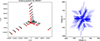 |
Fig. A.4. Antenna positions during the observations of J00418+4021 on 2020-12-04, and uv plane coverage of the L-band scan (with an averaging on 128 channels). |
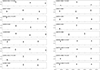 |
Fig. A.5. Sources variability across VLASS observations. Fluxes have been normalized by the maximum flux observed with VLASS, and the variability index V is shown for sources with detections in at least two epochs. |
Appendix B: Radio images properties, measured radio flux densities and spectrum, spectral indices and radio luminosity, IR and FIR fluxes
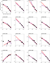 |
Fig. B.1. The radio spectra of the 16 sources detected in three bands or more. The dashed red line indicate the linear fit while the dashed purple line present the parabolic fit. Upper limits are shown but have been excluded during fitting procedure. The marker shape indicate the morphology of the source at the given frequency : circle for extended, square for intermediates and cross for compact sources. |
Final radio images properties*
Measured radio flux densities of the sources in mJy from the original images at their respective resolutions based on 5σ contours, their respective morphology type* and the calculated Kellermann’s parameter Rk.
IR and FIR fluxes used during the analysis.
Measured spectral indices and radio luminosity of the sources
Appendix C: Optical spectroscopy
Fig. C.1 shows the results of a multicomponent nonlinear analysis of the Hβ spectral range, after continuum subtraction. Several previous papers have successfully applied the same technique (Negrete et al. 2018); here we recall only the salient points. The main components of the model are a power law continuum, Fe II emission according to a standard template (Boroson & Green 1992), Hβ emission well-fit by a Lorentzian profile (see e.g., Sulentic et al. 2002; Shapovalova et al. 2012; Wang et al. 2014; Cracco et al. 2016; Negrete et al. 2018; Crepaldi et al. 2025, for a variety of approaches), and [OIII]λλ4959,5007 emission. In sources where Fe II is much weaker, the Lorentzian is found at a wavelength consistent with the one of the quasar rest frame; small shifts (≲ ± 100) are possible due to uncertainties in the systemic redshift (≲50 km s−1), compounded with a slight mismatch originating in the fitting process. The outflow emission originating from the broad-line region (BLR) is modeled as a blueshifted skew Gaussian, on the basis of the trapezoidal profile most often observed in the CIVλ1549 profile of xA sources (e.g., Zamanov et al. 2002; Leighly & Moore 2004; Martínez-Aldama et al. 2018). The narrow-line region (NLR) emission is similarly modeled by separating a symmetric Gaussian and a skew Gaussian (Azzalini 1985), usually shifted toward shorter wavelengths, and helpful to model the outflow component that is prominent in the [O III]λ5007 emission (Zhang et al. 2011). The shaded areas in Fig. C.1 emphasize the Hβ outflow profile (magenta) and the full blueshifted profile of [OIII]λλ4959,5007 (cyan). The Hβ BLUE (shaded magenta) is barely detectable in several sources, but produce are remarkable blueward asymmetry especially in the sources with strong Fe II emission. The [OIII]λλ4959,5007 full profile (shaded cyan) is often dominated by the SBC shifted to the blue. The [O III]λ5007 FWHM is large, and its equivalent width is low, to the point that the line is, in several cases, barely detectable over the strong Fe II emission. This result is in agreement with the basic tenet of the Eigenvector 1 paradigm (the anticorrelation between the peak intensity of [O III]λ5007 and RFeII, Boroson & Green 1992).
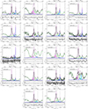 |
Fig. C.1. Continuum-subtracted, optical spectra of the 18 targets in the Hβ spectral range (upper panels). Abscissa is rest-frame wavelength (top scale) and radial velocity with respect to rest frame (bottom); ordinate is normalized specific flux, also in the rest frame. Thin black line: observed spectrum, thick black: broad component of Hβ; thick blue shaded cyan: full profile of [OIII]λλ4959,5007; magenta: Hβ broad blueshifted emission; grey: Hβ narrow component; pale green: Fe II template. The dashed magenta line traces the full empirical model of the spectrum. Lower panels: observed spectrum minus empirical model. |
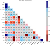 |
Fig. C.2. Correlation matrix (Pearson’s) involving the main optical (Hβ and [O III]λ5007), radio and IR derived parameters. The limits in the color ranges correspond to a statistical significance of ±1, 2, 3σ for the Pearson’s correlation coefficient computed for 18 objects. The parameters considered are in this order, the bolometric luminosity L, the black hole mass MBH, the Eddington ratio L/LEdd, the radio power at 1.4 GHz, the radio spectral index α, Fe II prominence ratio RFeII, the equivalent with of Hβ (broad components), its FWHM and centroid displacement at one-half peak intensity |


Table C.1 reports measurements carried out on full profile of the Hβ line, as well as on the blueshifted component associated with the BLR outflows. The centroids, the asymmetry (AI) and kurthosis (KI) indexes reported in the Tables are computed according to the definition of Zamfir et al. (2010). The column providing information on the strength of Fe II emission reports the intensity ratio RFeII = Fe IIλ4570/Hβ, where Fe IIλ4570 is the intensity of the blend on the blue side of Hβ (Fig. C.1), that is the parameter used for the selection of xA sources. The following columns report relative intensity normalized to the full broad profile of the Hβ broad component (BC), symmetric and unshifted, and its FWHM. For the blueshifted broad component (BLUE), the relative contribution is listed along with FWHM, peak shift and skew parameter that describes the asymmetry of the skew normal function used to model its profile.
Analysis of the Hβ and Fe IIλ4570 emission features
Table C.2 reports measurements carried out on the [O III]λ5007 line, following a scheme analogous to Table C.1 for Hβ. The centroids, AI and KI are reported for the full [O III]λ5007 profile following the spectrophotometric parameters. We distinguish a narrow component (NC) and a semi-broad component (SBC), with blueshifts ranging from almost 0 to a few thousands km s−1. We report relative intensity for the NC and SBC, along with FWHM and Shift. For the [O III]λ5007 SBC, the shift (defined as the mode of the skew normal distribution) is not representative of the bulk displacement of the line with respect to the rest frame. In this case, we provide also the centroid at half maximum  .
.
Profile analysis for [OIII]λ5007Å
C.1. Estimation of wind parameters
C.1.1. [OIII]λλ4959,5007
The large blueshifts and blue-ward skewness of the [OIII]λλ4959,5007 lines suggests the presence of an outflow for the emitting gas, possibly originating from nuclear winds, or from radiative feedback on the gas of the host galaxy bulge, where the receding side of the flow is obscured or absorbed (Zamanov et al. 2002; Cresci et al. 2015; Singha et al. 2022; Kakkad et al. 2022). The relations for line emitting gas mass, mass flow, thrust and kinetic power based on the BLUE component of [O III]λ5007 are the ones provided by Marziani et al. (2017), scaled to nH = 104 cm−3 (Sect. 3.6). They are standard relations (Cano-Díaz et al. 2012; Fiore et al. 2017), obtained assuming optically-thin emission confined in a bipolar outflow within a solid angle 2⋅Ω.
The immediate inference from the [O III]λ5007 outflow parameters (Tab. C.3) computed from the data listed in Table C.2 is that they show an especially strong dependence on luminosity, with the kinetic power reaching tenth of percent of the bolometric luminosity (∼0.1 − 0.2%) in the case of the most luminous sources. This result is consistent with previous works (Carniani et al. 2015; Fiore et al. 2017; Bischetti et al. 2017; Vietri et al. 2018; Kakkad et al. 2020). The mass outflow rate is always Ṁ ≲ 10 M⊙ yr−1, with only a few luminous sources reaching Ṁ ∼5 M⊙ yr−1. The low values of the wind parameters are also a consequence of the low equivalent width of the [O III]λ5007 emission (Boroson & Green 1992; Zamanov et al. 2002). Apparently, even if the sources of the present sample are close to maximum radiative output per unit black hole mass, they are capable of inducing modest mechanical effects, especially at low-luminosity.
Mass outflow rates and kinetic powers
C.1.2. Hβ
An estimation of the wind parameters for Hβ BLUE is less standard, as the mildly-ionized wind emission has been usually traced by the resonance high-ionization line of CIVλ1549 (e.g., Marziani et al. 2016a; Vietri et al. 2018). The blueshifted Hβ emission is presumably associated with the BLR: spatial scales are smaller, and the electron densities are expected to be much higher with respect to the [O III]λ5007 emitting regions, but are less well-known. It is customary to assume a standard value for the BLR electron density n ∼ 109 > 108 cm−3 (Netzer 2013), even if the density of the low-ionization part of the BLR is much higher (Marziani et al. 2010; Negrete et al. 2012; Temple et al. 2020, 2021), ∼1012 − 1013 cm−3, and the outflow might be clumpy (e.g., Ward et al. 2024). The Hβ emissivity can be written as  where n is the Hydrogen density (ne ∼ nH ∼ n) and αHβ(T) is the effective recombination coefficient for Hβ. At Te = 20000 K, αHβ ≈ 3.8 × 10⁻¹⁴ cm3 s−1 (Osterbrock & Ferland 2006), yielding an Hβ emissivity jHβ ∼ 1.23 ⋅ 10−7n92 erg s−1 cm−3. Therefore, the total mass of the line emitting gas is
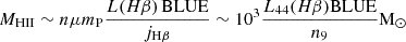
where we assume nH = 109 cm−3, the molecular weight μ = 1.4, and mP is the proton mass.
Using the same approach applied to [O III]λ5007, we can compute the outflow’s dynamical parameters as traced by the Hβ line. In this scenario, the gas emitting Hβ is presumably still being accelerated by radiation pressure, thereby gaining momentum. An additional factor must be incorporated into these calculations, either by adopting a simplified model for an unbound gas subject to gravity and radiation pressure (Netzer & Marziani 2010; Marziani et al. 2017) or by applying an empirical recipe developed for the CIVλ1549 line (Deconto-Machado et al. 2024), assuming a final outflow velocity of  for the blueshifted component. We apply the simplest assumption including a factor κ = 5 (Marziani et al. 2017). The resulting relations for line emitting mass, mass flow, thrust and kinetic power based on the BLUE component of Hβ are:
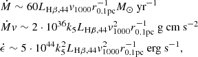
assuming nH = 109 cm3, and velocity scaled to 1000 km s−1.
The results obtained for the BLR outflow traced by the blueshifted excess of the Hβ line, reported in Table C.3, are consistent with the ones for the [O III]λ5007 outflow. In the Hβ case, there is however no straightforward comparison with earlier results based on the same line: the BLUE component is faint and difficult to measure, especially in cases with strong Fe II. Since Hβ BLUE should be emitted in the same mildly-ionized outflow producing CIVλ1549 and other UV high-ionization lines, a comparison can be made with the outflow parameters derived from CIVλ1549 (Marziani et al. 2016b; Vietri et al. 2018; Deconto-Machado et al. 2023, 2024). The mass outflow rate is Ṁ ∼ 1 ≲ a few M⊙ yr−1, with only J13012+5902 reaching Ṁ ∼ 40 M⊙ yr−1. Even if these values could be considered more as lower limit as anything else, the basic outcome is again consistent with previous results, where only at the largest luminosities the kinetic power might become as large as to imply a significant feedback effect on the host galaxy (Di Matteo et al. 2005; Ishibashi & Fabian 2012; King & Pounds 2015; Harrison et al. 2014; King & Muldrew 2016; Laha et al. 2020). The implication is that, while these sources are mostly candidate super-Eddington quasars, their BLR winds do not necessarily produce the strongest feedback, as the feedback effect primarily depends on luminosity – and thus on black hole mass – if L/LEdd ≳0.2 (Marziani et al. 2025): L/LEdd is constrained to be L/LEdd ≲1 (Mineshige et al. 2000), and hence to vary within a small range. On the converse MBH and AGN luminosity (to which line luminosity is roughly proportional) can be factors ∼ 100 higher in the most luminous quasars at the cosmic noon. Only in those cases the mechanical power of the NLR and BLR winds may reach values close to the ones needed for a global effect on the host galaxy (Deconto-Machado et al. 2023).
C.2. Accretion parameters
The black hole masses are computed assuming virial broadening for the emission lines: MBH = frBLRFWHM2/G, where f is the virial factor and rBLR the radius of the emitting region (e.g., Vestergaard & Peterson 2006; Shen 2013). The dependence of f on the viewing angle has been parameterized by Mejía-Restrepo et al. (2018) as f≈ (FWHM/4550)−1.17, and the rBLR dependence on Eddington ratio by applying a correction to the standard scaling between rBLR and optical luminosity at 5100 Å (Du & Wang 2019; Martínez-Aldama et al. 2020).
The main empirical correlation with Eddington ratio is the RFeII prominence parameter (e.g., Sulentic et al. 2000b; Marziani et al. 2001; Sun & Shen 2015; Du et al. 2016; Panda et al. 2019), defined as the ratio between the fluxes of the Fe II blend centered at 4570 Å and Hβ. The parameter RFeII is one of the two main parameters (along with FWHM Hβ) defining the quasar Eigenvector 1 main sequence (Boroson & Green 1992; Sulentic et al. 2000b). The classical scaling law linking BLR distance rBLR from AGN continuum to luminosity (Bentz et al. 2009) shows a dependence on Eddington ratio (Martínez-Aldama et al. 2020). A tight relation between rBLR and luminosity can be recovered once rBLR is corrected, using the robust measurement of RFeII in place of L/LEdd. The following relation (Du & Wang 2019):
![Mathematical equation: $$ \begin{aligned} \log r_{\rm BLR} \approx 17.063 + 0.45 \log L_{5100,44} - 0.35 R_{\rm FeII}\ \mathrm{[cm],} \ \end{aligned} $$](/articles/aa/full_html/2026/03/aa57025-25/aa57025-25-eq49.gif) (C.1)
(C.1)
yields:
![Mathematical equation: $$ \begin{aligned} \log M_{\rm BH}(\mathrm{H} \beta )&\approx { 5.220} + 0.45 \log L_{5100,44} + \nonumber \\&0.83 \log \mathrm{FWHM} - 0.35 R_{\rm FeII} \, [\mathrm{M} _\odot ]. \end{aligned} $$](/articles/aa/full_html/2026/03/aa57025-25/aa57025-25-eq50.gif) (C.2)
(C.2)
Eq. (C.2) implies a significant increase of the MBH values for the sources with the narrowest profile with respect to the scaling law of Vestergaard & Peterson (2006), providing estimates in closer agreement with the ones obtained from more robust methods (D’Onofrio et al. 2024). The systematic MBH uncertainty is estimated by computing the dispersion between the MBH values computed from Eq. (C.2) and three different scaling laws, of them two based on the Hβ line width (Vestergaard & Peterson 2006; Shen et al. 2024), and one on the Hβ luminosity (Greene & Ho 2005): δlog MBH ≈0.17, with a negligible bias between MBH from Eq. (C.2) and the average of the other scaling laws, δlog MBH ≈ −0.05 ± 0.20. The uncertainty associated with the scaling law is still dominating with respect to the statistical uncertainties in line FWHM and in continuum flux measurement, ≲10% at 1σ confidence level.
The bolometric correction (BC) was computed accounting for its dependence on luminosity (Runnoe et al. 2012). We utilize the BC parameterization by Netzer (2019) that are fairly consistent, at low luminosity, with the ones described for highly accreting quasars: for Eddington ratios in the range log L/LEdd ∼ − 0.5 − 0.0, at log λLλ(5100 Å)∼43 − 44 [erg s−1] the bolometric correction has been estimated between 16 and 23 (Garnica et al. 2025) and 10 and 18.8 (Ferland et al. 2020). If the Garnica et al. and the Netzer (2019) bolometric corrections are applied to the present sample, the systematic difference in bolometric luminosity L is negligible, ≈12%. Results for optical and bolometric luminosity, and for MBH and L/LEdd are reported in Table C.4.
Accretion parameters
Table C.5 reports statistical and systematic linear fractional uncertainties for the accretion parameters. The main source of uncertainty is the systematic uncertainty associated with the different scaling laws employed for MBH estimates. The uncertainty is apparently reduced with respect to earlier works (Vestergaard & Peterson 2006), but is still affecting heavily the MBH and L/LEdd estimates. If systematic and statistical errors are quadratically propagated (column Total in Table C.5), the uncertainties reach values ≳70 % for the L/LEdd, δlog L/LEdd ∼ ± 0.32, an aspect that should be considered in any correlation analysis involving L/LEdd.
Statistical and systematic linear fractional uncertainties for the accretion parameters
All Tables
Measured radio flux densities of the sources in mJy from the original images at their respective resolutions based on 5σ contours, their respective morphology type* and the calculated Kellermann’s parameter Rk.
Statistical and systematic linear fractional uncertainties for the accretion parameters
All Figures
|
Fig. 1. Prevalence of FIRST-detected type 1 AGNs (Marziani et al. 2013) (blue circles and cyan shading) and median radio power (red circles and pink shading) as a function of spectral type along the quasar main sequence. |
| In the text | |
|
Fig. 2. Radio morphology distribution across source redshifts. The letter C indicates compact emission at all observed frequencies, I indicates intermediate morphology detected in at least one band, and E indicates the presence of diffuse emission in at least one band. |
| In the text | |
|
Fig. 3. Spectral indices plotted as α1.5 − 5 vs. α0.144 − 1.5, α3 − 5 vs. α1.5 − 3, α5 − 10 vs. α3 − 5, and α5 − 10 vs. α1.5 − 5. Markers are colored according to the dominating mechanism responsible for the detected radio emission (Table 2). The dashed line indicates the 1 : 1 ratio of equal slopes, while the horizontal and vertical dotted lines correspond to α = −0.5. The region showing flat or inverted spectra, which may be associated with a core-dominated jet or a corona, is shaded gray. The region with a spectral index α = −0.8 ± 0.4 and a scatter of 0.2, possibly related to SF, is shaded turquoise. The region showing very steep spectral slopes with α5 − 10 < −2 in the right-hand panel, which may imply possible relic emission, is shaded blue. |
| In the text | |
|
Fig. 4. Two-point spectral index between radio (1.4 GHz) and mid-IR (22 μm). All sources have |
| In the text | |
|
Fig. 5. Star formation rate (SFR) estimate from FIR luminosity vs. radio pseudo-SFR for all sources radio-detected and with IRAS 60 μm data (black diamonds). Star-forming galaxies (green circles), RQ quasars (blue circles) and RL quasars (pink circles) are from Bonzini et al. (2015), with their pSFRradio converted using Eq. 22 of Molnár et al. (2021). The dashed line is the 1:1 ratio line of equal SFR. |
| In the text | |
|
Fig. 6. Summary of the classification scheme used to identify the dominant radio emission mechanism for each sources in our sample, based on the combination of indicators compiled in Table 2. |
| In the text | |
|
Fig. 7. Spectral index α5 − 10 vs. the Eddington ratio, the FWHM of the Hβ line (in km/s), the flux ratio RFeII, and MBH. Markers are colored according to the dominant mechanism responsible for the detected radio emission (Table 2). Blue and pink filled circles indicate RQ and RL quasars, respectively, from Laor et al. (2019). |
| In the text | |
|
Fig. 8. Results of the PCA analysis. Top: 1D projection of sources along the PC1. Bottom: Vector loading along the PC1. |
| In the text | |
|
Fig. A.1. LOFAR (144 MHz) - when available - as well as our VLA L (1.5 GHz), C (5 GHz) and X (10 GHz) band images and VLASS (S-band, 3 GHz) of the 18 targets of the sample, each with a 5σ contour encompassing the main target in white. The sizes of the beams are shown in the bottom-left corner, while the scales are in the bottom-right corner. The cutouts have sizes of 1′×1′, 20″ × 20″, 20″ × 20″, 6″ × 6″ and 4″ × 4″ at 144 MHz, 1.5 GHz, 3 GHz, 5 GHz and 10 GHz respectively - except for sources with larger detected diffuse emission (J00418+4021, J12562+5652), which cutouts have been increased to encompass it. |
| In the text | |
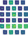 |
Fig. A.2. Continuation of Figure A.1. |
| In the text | |
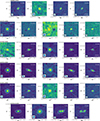 |
Fig. A.3. Continuation of Figure A.1. |
| In the text | |
|
Fig. A.4. Antenna positions during the observations of J00418+4021 on 2020-12-04, and uv plane coverage of the L-band scan (with an averaging on 128 channels). |
| In the text | |
|
Fig. A.5. Sources variability across VLASS observations. Fluxes have been normalized by the maximum flux observed with VLASS, and the variability index V is shown for sources with detections in at least two epochs. |
| In the text | |
|
Fig. B.1. The radio spectra of the 16 sources detected in three bands or more. The dashed red line indicate the linear fit while the dashed purple line present the parabolic fit. Upper limits are shown but have been excluded during fitting procedure. The marker shape indicate the morphology of the source at the given frequency : circle for extended, square for intermediates and cross for compact sources. |
| In the text | |
|
Fig. C.1. Continuum-subtracted, optical spectra of the 18 targets in the Hβ spectral range (upper panels). Abscissa is rest-frame wavelength (top scale) and radial velocity with respect to rest frame (bottom); ordinate is normalized specific flux, also in the rest frame. Thin black line: observed spectrum, thick black: broad component of Hβ; thick blue shaded cyan: full profile of [OIII]λλ4959,5007; magenta: Hβ broad blueshifted emission; grey: Hβ narrow component; pale green: Fe II template. The dashed magenta line traces the full empirical model of the spectrum. Lower panels: observed spectrum minus empirical model. |
| In the text | |
|
Fig. C.2. Correlation matrix (Pearson’s) involving the main optical (Hβ and [O III]λ5007), radio and IR derived parameters. The limits in the color ranges correspond to a statistical significance of ±1, 2, 3σ for the Pearson’s correlation coefficient computed for 18 objects. The parameters considered are in this order, the bolometric luminosity L, the black hole mass MBH, the Eddington ratio L/LEdd, the radio power at 1.4 GHz, the radio spectral index α, Fe II prominence ratio RFeII, the equivalent with of Hβ (broad components), its FWHM and centroid displacement at one-half peak intensity |
| In the text | |
Current usage metrics show cumulative count of Article Views (full-text article views including HTML views, PDF and ePub downloads, according to the available data) and Abstracts Views on Vision4Press platform.
Data correspond to usage on the plateform after 2015. The current usage metrics is available 48-96 hours after online publication and is updated daily on week days.
Initial download of the metrics may take a while.