| Issue |
A&A
Volume 707, March 2026
|
|
|---|---|---|
| Article Number | A89 | |
| Number of page(s) | 13 | |
| Section | Astrophysical processes | |
| DOI | https://doi.org/10.1051/0004-6361/202557029 | |
| Published online | 27 February 2026 | |
Identifying massive black hole binaries via light curve variability in optical time-domain surveys
1
Dipartimento di Fisica “G. Occhialini”, Università degli Studi di Milano-Bicocca Piazza della Scienza 3 20126 Milano, Italy
2
INFN, Sezione di Milano-Bicocca Piazza della Scienza 3 20126 Milano, Italy
3
Como Lake Center for Astrophysics, DiSAT, Università degli Studi dell’Insubria Via Valleggio 11 22100 Como, Italy
4
Dipartimento di Fisica “A. Pontremoli”, Università degli Studi di Milano Via Giovanni Celoria 16 20134 Milano, Italy
5
Donostia International Physics Centre (DIPC) Paseo Manuel de Lardizabal 4 20018 Donostia-San Sebastian, Spain
6
IKERBASQUE, Basque Foundation for Science E-48013 Bilbao, Spain
★ Corresponding author: This email address is being protected from spambots. You need JavaScript enabled to view it.
Received:
29
August
2025
Accepted:
17
December
2025
Abstract
Accreting massive black hole binaries (MBHBs) often display periodic variations in their emitted radiation, thus providing a distinctive signature for their identification. For this work we explored the identification of MBHBs via optical variability studies by simulating the observations of the Vera C. Rubin Observatory’s Legacy Survey of Space and Time (LSST). To this end, we generated a population of MBHBs using the L-Galaxies semi-analytical model, focusing on systems with observed orbital periods ≤5 years. This ensures that at least two complete cycles of emission could be observed within the ten-year mission of LSST. To construct mock optical light curves, we first calculated the MBHB average magnitudes in each LSST filter by constructing a self-consistent spectral energy distribution that accounts for the binary accretion history and the emission from a circumbinary disc and mini-discs. We then added variability modulations by using six 3D hydrodynamic simulations of accreting MBHBs with different eccentricities and mass ratios as templates. To make the light curves more realistic, we mimicked the LSST observation patterns and cadence, and we included stochastic variability and LSST photometric errors. Our results show from 10−2 to 10−1 MBHBs per square degree, with light curves that are potentially detectable by LSST. These systems are mainly low-redshift (z ≲ 1.5), massive (M ≳ 107 M⊙), of equal mass (q ≈ 0.9), and relatively eccentric (e ≈ 0.6), and have modulation periods of around 3.5 years. Using periodogram analysis, we find that LSST variability studies have a higher success rate (≳50%) for systems with high eccentricities (e ≳ 0.6). Additionally, at fixed eccentricity, detections tend to favour systems with more unequal mass ratios. The false alarm probability (FAP) shows similar trends. Circular binaries systematically feature high FAP values (≳10−1). Eccentric systems have low-FAP tails, down to ≈10−8.
Key words: black hole physics / methods: numerical / quasars: supermassive black holes
© The Authors 2026
 Open Access article, published by EDP Sciences, under the terms of the Creative Commons Attribution License (https://creativecommons.org/licenses/by/4.0), which permits unrestricted use, distribution, and reproduction in any medium, provided the original work is properly cited.
This article is published in open access under the Subscribe to Open model. This email address is being protected from spambots. You need JavaScript enabled to view it. to support open access publication.
1. Introduction
It has been observationally established that massive galaxies host a massive black hole (MBH, mass MBH ≳ 106 M⊙) at their centres (see e.g. Schmidt 1963; Genzel & Townes 1987; Kormendy & Richstone 1992; Hopkins et al. 2007; Merloni & Heinz 2008; Aird et al. 2015). While the origin and initial growth of MBHs remain unclear, observational evidence reveals correlations between the properties of MBHs and those of their host galaxies. These trends suggest a co-evolution in their growth histories (Haehnelt & Rees 1993; O’Dowd et al. 2002; Haring & Rix 2004; Kormendy & Ho 2013; Savorgnan et al. 2016). Such findings are consistent with the widely accepted hierarchical structure formation model, where galaxy interactions play a crucial role in the assembly of galaxies and the growth of MBHs (Press & Schechter 1974; White & Rees 1978; Di Matteo et al. 2005).
The hierarchical assembly of galaxies, together with the existence of MBHs implies that massive black hole binary (MBHB) systems form naturally in the Universe. Although the evolution of these MBHBs is difficult to probe observationally, it has been theoretically shown to proceed in different phases (Begelman et al. 1980). After two galaxies merge, their central MBHs sink towards the nucleus of the remnant galaxy via dynamical friction. Once deep within the remnant galaxy, the two objects form a gravitationally bound binary system which continues to evolve towards coalescence via interactions with surrounding stars or a circumbinary disc, and through the emission of gravitational waves (Peters & Mathews 1963; Quinlan & Hernquist 1997; Escala et al. 2004, 2005; Sesana et al. 2006; Dotti et al. 2007; Cuadra et al. 2009; Vasiliev et al. 2014; Sesana & Khan 2015; Biava et al. 2019; Bonetti et al. 2020; Franchini et al. 2021, 2022).
The detection of a large population of MBHBs would represent a crucial step for understanding how galaxies assemble as well as the origins of MBHs, given the tight connection between the galactic host and its central MBH. Despite its relevance, direct observational confirmation of MBHBs remains challenging because of their small angular separations. Traditional detection methods rely on spatially-resolved pairs of active galactic nuclei (AGNs) or quasars (i.e. dual AGNs). However, these methods target pairs of MBHs separated by more than a few parsecs, which correspond to scales much larger than those at which the MBHs become gravitationally bound (Wang et al. 2009; Koss et al. 2012; Comerford et al. 2012; Orosz & Frey 2013; Comerford & Greene 2014; Müller-Sánchez et al. 2015; Hwang et al. 2020; Ciurlo et al. 2023). An alternative avenue to asses the detectability of MBHBs involves the detection of the variable electromagnetic emission coming from AGNs (Graham et al. 2015a; D’Orazio & Loeb 2018; De Rosa et al. 2019; D’Orazio & Charisi 2023; Luo et al. 2024; Tubín-Arenas et al. 2025). Different hydrodynamic simulations have shown that accreting MBHBs feature periodic modulations in their electromagnetic emission (see e.g Artymowicz & Lubow 1994, 1996; Hayasaki et al. 2007; Roedig et al. 2011; D’Orazio et al. 2013; Farris et al. 2014; Muñoz & Lai 2016; Franchini et al. 2024; Cocchiararo et al. 2024). These variations arise from the mutual gravitational interaction between the two MBHs, which induces changes in the behaviour and properties of the gas that is funnelled towards them. In addition to hydrodynamic variability, other processes can lead to periodic changes in the emission from MBHBs. One of these is the relativistic Doppler effect, which occurs as the MBHs orbit each other. This effect can cause the emitted radiation (such as broad emission lines) to be blueshifted or redshifted, resulting in observable fluctuations in brightness and spectral features (D’Orazio et al. 2015; Charisi et al. 2018; Dotti et al. 2023; Ge et al. 2024; Bertassi et al. 2025).
Given the points above, many studies have analysed data from large time-domain optical surveys of quasars and AGNs to identify candidates for MBHBs. For instance, Graham et al. (2015b) identified 100 variable quasars by using the data of the Catalina Real-Time Transient Survey (CRTS). Similarly, Charisi et al. (2016) reported a few dozen candidates from the Palomar Transient Factory (PTF). Although these searches are a promising approach, the identification of periodic variability in quasars is particularly challenging as quasars also exhibit stochastic variability, well-described by a damped random walk model (Kelly et al. 2009; Kozłowski et al. 2010; MacLeod et al. 2010). These signals can resemble the natural variability of MBHBs, leading to the selection of false candidates (Vaughan et al. 2016). Ongoing surveys such as the Vera C. Rubin Observatory’s Legacy Survey of Space and Time (LSST, Ivezić et al. 2019) and the Zwicky Transient Facility (ZTF, Dekany et al. 2020) will provide unprecedentedly large, high-cadence, and high-sensitivity datasets, thus improving our ability to distinguish genuine periodic signals from stochastic variability.
With this in mind, the aim of this project was to study the capabilities of the LSST survey to identify MBHBs through variability studies. To this end, we used a population of simulated MBHBs extracted from a lightcone generated by the L-Galaxies semi-analytical model (Henriques et al. 2015; Izquierdo-Villalba et al. 2023). We created mock optical light curves for our simulated MBHBs. To this end, we relied on L-Galaxies to estimate the average emission of the individual sources. We then modelled their variability fluctuations by using six 3D hyper-Lagrangian resolution hydrodynamic simulations of accreting MBHBs as templates (Cocchiararo et al. 2024). We then implemented the MBHB stochastic variability, LSST photometric errors, and the LSST observation pattern and cadence. These light curves then underwent a periodogram analysis to assess the LSST success rate in detecting MBHBs and to estimate false alarm probabilities.
This paper is organised as follows. Section 2 describes the LSST survey, the L-Galaxies semi-analytical model and the selected population of MBHBs. Section 3 describes the model used to determine the spectral energy distribution of our MBHBs, together with the properties of MBHBs detected by LSST. Section 4 presents the methodology followed to construct realistic MBHB light curves and the LSST success rate and false alarm probability. In Section 5 we present the results of our analysis. Section 6 discusses some potential caveats related to the results. Finally, in Section 7 we summarise our main findings. A ΛCDM cosmology with parameters Ωm = 0.315, ΩΛ = 0.685, Ωb = 0.045, σ8 = 0.9, and H0 = 67.3 km s−1 Mpc−1 is adopted throughout the paper (Planck Collaboration XVI 2014).
2. Building a simulated sky
In this section we describe the chosen optical survey for conducting MBHB searches and the theoretical model employed to generate simulated populations of galaxies, MBHs, and MBHBs.
2.1. The Vera Rubin Observatory
We explore the detectability of the optical variability of MBHBs, by simulating the observations of the Vera C. Rubin Observatory’s Legacy Survey of Space and Time (LSST). This mission is expected to operate for 10 years and cover ∼18 000 deg2 in the u, g, r, i, z, y optical bands, spanning over the 320 − 1100 nm range (Ivezić et al. 2019). The extensive area covered, combined with the anticipated observing cadence of approximately three to four nights, enables LSST to reach deep magnitudes across all filters, facilitating the detection of faint AGNs and supporting variability studies. The effective wavelength of each filter and its detection limits are presented in Table 1. We particularly emphasise that our main focus is on the magnitude limits achievable in LSST single-exposure mode as these are essential for enabling multi-epoch analyses required for variability searches.
Sensitivity and effective wavelength of the LSST filters.
2.2. The L-Galaxies semi-analytical model
To produce a simulated population of galaxies, MBHs and MBHBs, we use the state-of-the-art L-Galaxies semi-analytical model (SAM). Indeed, L-Galaxies is tuned to reproduce many observables like stellar mass functions, star formation rate density or galaxy colours (see Henriques et al. 2015 for further details). Among all the versions of the model, we use the one presented in Izquierdo-Villalba et al. (2023).
2.2.1. Dark matter merger trees
L-Galaxies is a SAM based on the dark matter (DM) merger trees extracted from N-body DM-only simulations (Springel 2005). In this work, we use the Millennium-II simulation (MSII) which tracks the cosmological evolution of 21603 DM particles with mass 6.885 × 10⁶ M⊙/h within a periodic comoving box of 100 Mpc/h on a side (Boylan-Kolchin et al. 2006). MSII was stored at 68 different epochs or snapshots, in which the SUBFIND algorithm was applied to detect all the DM halos whose minimum halo mass corresponds to 20 times the particle mass. These halos were sorted by progenitors and descendants in the so-called merger tree structure by applying the L-HALOTREE code. Finally, the procedure of Angulo & White (2010) was applied to the outputs of MSII to re-scale the original cosmology to the one provided by Planck Collaboration XVI (2014).
2.2.2. Galaxy formation
Regarding the baryonic processes, L-Galaxies follows the standard assumption of White & Frenk (1991) which assumes that the birth of a galaxy takes place at the centre of every newly formed DM halo. During the spherical collapse of the DM halo, a fraction of baryonic matter is trapped and collapses with it. During this process, the baryons are shock-heated, causing the formation of a diffuse, spherical, and quasi-static hot gas atmosphere with an extension equal to the halo virial radius. Gas is then allowed to cool down and migrate towards the centre of the DM halo, forming a disc structure capable of triggering star formation as soon as a certain critical mass is reached. These events result in the formation of the galaxy stellar disc, whose evolution is regulated by supernova feedback of massive stars which release energy and metals into the interstellar medium. Stellar discs can also give rise to compact concentrations of stars at the centre of the galaxy, called galactic bulges. During cosmic evolution, the disc can be affected by secular (disc instabilities) and external processes (galaxy mergers), resulting in the formation of nuclear stellar concentrations called bulges. L-Galaxies also takes into account environmental processes such as hot gas stripping or tidal disruption. For further details of the baryonic physics, we refer to Henriques et al. (2015). Finally, we note that L-Galaxies performs an internal time interpolation of ∼15 Myr between two consecutive MSII snapshots to enhance the accuracy of the baryon evolution.
2.2.3. Massive black holes
Although the latest version of L-Galaxies features a sophisticated model for MBH formation (Pop III remnants, direct collapse of pristine gas clouds and runaway stellar mergers, see Spinoso et al. 2023), the version used in this work employs the simpler assumptions outlined in Izquierdo-Villalba et al. (2023). In short, when a new DM halo is resolved, L-Galaxies assigns to it a probability to host an MBH seed depending on its mass and redshift. The mass and spin of the seed are chosen randomly from 102 − 104 M⊙ and 0 − 0.998, respectively. The seeding process is active down to z = 7, when star formation processes have polluted enough the intercluster medium to inhibit any further MBH formation event (Spinoso et al. 2023). Once the MBH is formed, its growth can occur via three different processes: cold gas accretion, hot gas accretion and coalescence with other MBHs. Among these, the former is the most important channel and is triggered after galaxy mergers or disc instability processes. During these events, part of the cold gas flows towards the galaxy centre and settles in a reservoir around the MBH (Izquierdo-Villalba et al. 2020). This reservoir is progressively consumed according to a two-phase model (Hopkins et al. 2005, 2006; Marulli et al. 2006; Bonoli et al. 2009). The first phase corresponds to an Eddington limit growth, which lasts until 70% of the available gas is consumed. Then the MBH enters a self-regulated phase characterised by sub-Eddington accretion rates (Hopkins & Hernquist 2009). Finally, L-Galaxies also tracks the evolution of the MBH spin. During gas accretion events, the model follows the approach described by Sesana et al. (2014), while during MBH coalescences, the final spin is determined as in Barausse & Rezzolla (2009).
2.2.4. Massive black hole binaries
After a galaxy-galaxy merger, L-Galaxies tracks the three-stage evolution of MBHBs (Begelman et al. 1980). The first stage is dominated by dynamical friction, and lasts until the MBH of the satellite galaxy reaches the centre of its new host galaxy. During this phase, the MBHs can grow by progressively accreting the gas reservoir that was already present before the merger. This gas reservoir includes all the material the MBH had accumulated prior to the galaxy interaction (via disc instabilities or previous mergers) as well as an additional amount collected at the time of the merger (Capelo et al. 2015). Once the dynamical friction phase is over, the satellite MBH reaches the nucleus of the galaxy and binds gravitationally with the central MBH. At this moment, a MBHB forms and the system enters the so-called hardening phase. In this stage, the separation (aBHB) and eccentricity (eBHB) of the binary system are tracked numerically depending on the environment in which the binary is embedded. If the gas reservoir around the binary is smaller than its total mass, the evolution of the system is driven by the interaction with single stars embedded in a Sérsic profile (hereafter, stellar hardening). Otherwise, the system evolves thanks to the interaction with a circumbinary gaseous disc (hereafter, gas hardening). We note that during the gas hardening, and as long as the GW emission is subdominant, the model follows the results from Roedig et al. (2011) and fixes the eccentricity of the MBHB to a stable value of 0.6 (see Murray & Duffell 2025, for further advances in the equilibrium eccentricity of accreting MBHBs). This assumes that the transient phase to get to eccentricity equilibrium is shorter than the circumbinary disc lifetime, which is generally the case since the time it takes to reach equilibrium is generally ≲3 Myr (Siwek et al. 2023), while the gas reservoir lasts for > 10 Myr. As the gas reservoir is exhausted, the MBHB evolution reverts to the stellar hardening prescription. Finally, when the separation between the two MBHs becomes small enough, the system enters the GW-dominated phase, which brings the two MBHs to the eventual merger. During this phase, the code tracks the evolution of aBHB and eBHB according to Peters & Mathews (1963). We note that our model can reproduce the GW background measurements that are currently observed using Pulsar-Timing Arrays (PTAs).
L-Galaxies models the gas accretion process onto hard MBHBs following the results of Duffell et al. (2020):
 (1)
(1)
Here qBHB = M2 / M1 is the binary mass ratio, with M1 and M2 the mass of the primary (most massive) and secondary (less massive) black hole. Their accretion rates are, respectively, Ṁ1 and Ṁ2. Given Eq. (1), the default strategy of L-Galaxies is to initially set the secondary MBH at its Eddington limit, while the primary MBH receives what is left of the reservoir that is being accreted onto the MBHB. We note that this strategy allows us to reproduce the quasar luminosity function at different redshift ranges. The details regarding the handling of MBHBs in L-Galaxies are presented in Izquierdo-Villalba et al. (2022).
2.2.5. A tailored simulated lightcone for the LSST
To make accurate theoretical predictions about the detectability of MBHBs with LSST, we do not use the standard comoving galaxy boxes generated by L-Galaxies at various redshifts. Instead, we utilise the lightcone outputs1 described in Izquierdo-Villalba et al. (2023). For simplicity, we only highlight the main features of the lightcone and refer to Izquierdo-Villalba et al. (2023) for detailed information about its construction. The lightcone, created using the version of L-Galaxies described before, follows a line of sight at coordinates (RA, Dec) = (77.1, 60.95) deg and includes all simulated galaxies up to z ≈ 3.5. The sky footprint has a rectangular shape covering an area of (δRA, δDec) = (45.6, 22.5) deg, which corresponds to ∼1026 deg2.
Out of the approximately ∼1.7 × 10⁸ galaxies contained in the lightcone, in this work we focus on those hosting MBHBs whose observed orbital period, Pobs = (1 + zBHB)×P, satisfies
 (2)
(2)
where G is the gravitational constant and MBHB, aBHB and zBHB are, respectively, the MBHB mass, semi-major axis, and redshift. The condition presented in Eq. (2) is introduced to ensure an effective periodicity study of the MBHB light curve through the LSST photometric observations. Since MBHBs are expected to show some periodic features in their emission related to their Keplerian frequency, it is important to select systems for which these periodic signals can be reliably detected within the entire LSST mission lifetime. Given the 10 yr duration of the LSST survey (Ivezić et al. 2019), we require that at least two complete MBHB emission cycles be sampled. As a result, this condition limits our sample to a catalogue of ≈6.5 × 10⁵ MBHBs within the lightcone simulated volume. Therefore, unless otherwise stated, the parent MBHB population studied in this work is restricted to the objects with Pobs ≤ 5 yr. For the sake of clarity, in Fig. 1 we show a slicing of the lightcone, together with the MBHBs hosted in it. We also show the light curves of a selected MBHB in LSST, in its u, g, r, i, z, i, and y filters. The light curve construction is described in detail in the next sections.
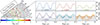 |
Fig. 1. Left panel: Thin slice of the simulated light cone. The coloured points correspond to MBHBs with Pobs ≤ 5 yr, while the black points represent all other galaxies hosted in the lightcone. We note that the lightcone slice shows some spatial periodicity of structures, which results from the box replication needed to build a wide and deep lightcone with the MSII merger trees. Right panels: Light curves in the LSST bands (u, g, r, i, z, y) associated with a MBHB at redshift ∼1.22 with mass ∼7.3 × 10⁷ M⊙, mass ratio ∼0.77 and eccentricity ∼0.24. The error bars correspond to the associated photometric uncertainty. The modelling and construction of the MBHB emission is illustrated in detail in Sections 3–4. |
3. The EM emission of inspiralling MBHBs
Although L-Galaxies can track the accretion history of MBHs and MBHBs, it does not include a model to determine their spectral energy distribution (SED). To address this, in this section we describe the approach used to model the SEDs of active MBHBs (see also Truant et al. 2026). Additionally, we outline how the resulting emission is measured by the different LSST filters. Lastly, we illustrate the properties of the MBHBs that are within the Vera Rubin Observatory detection capabilities.
3.1. Spectral energy distribution of a MBHB
It has been shown that mergers and disc instabilities can make gas on large scales lose its angular momentum and fall towards the galactic centre where MBHs and MBHBs reside (Hopkins & Quataert 2010). Despite that, it is likely that the gas which reaches the vicinity of MBHs retains some angular momentum, causing the formation of an accretion disc or, in the case of MBHBs, a circumbinary disc (see e.g. Ivanov et al. 1999; Haiman et al. 2009; Lodato et al. 2009; Goicovic et al. 2016). For this latter case, the gravitational torque exerted by MBHB on the gas disc causes the opening of a large cavity around the two MBHs (MacFadyen & Milosavljević 2008; D’Orazio et al. 2016). Despite the presence of this gap, some gas streams can still flow inside the cavity and onto each MBH, leading to the formation of mini-disc structures (Artymowicz & Lubow 1996; Ragusa et al. 2016; Fontecilla et al. 2017; Franchini et al. 2022, 2023).
To estimate the electromagnetic emission of our selected MBHB population, we approximate its spectral energy distribution (SED, Lν) as the sum of three different components:
 (3)
(3)
Here  represents the contribution of the mini-disc surrounding the primary (i = 1) or secondary (i = 2) MBH and
  corresponds to the emission from the circumbinary disc (CBD). This approach follows the strategy of other authors, such as Tiede & D’Orazio (2025), and manages to capture most of the MBHB average emission. We note that, for simplicity, we do not model the emission of any other structure, such as gas streams (see e.g. Fig. 2 of Cocchiararo et al. 2024). In the following paragraphs, we outline the methodology used to describe the three components.
(a) Circumbinary disc – This component is modelled according to a thin disc model (TD, Shakura & Sunyaev 1973),
![Mathematical equation: $$ \begin{aligned} L_{\nu } = 2 \pi \, h\, r_{\rm S} \,\frac{\nu ^{3}}{c^{2}} \ \int \limits _{x_{\rm in}}^{x_{\rm out}}{4 \pi x \left[\mathrm{exp}\left(\frac{h \nu }{k_{\rm B} \, T(x)}\right)-1 \right]^{-1} \mathrm{d}x}, \end{aligned} $$](/articles/aa/full_html/2026/03/aa57029-25/aa57029-25-eq6.gif) (4)
(4)
where x ≡ r/rS. Here, r is the radial distance to the MBH, rS the Schwarzschild radius, kB the Boltzmann constant, h the Planck constant, c the speed of light, and ν the rest-frame frequency. The quantity T(x) represents the temperature of the accretion disc at a given distance x from the MBHB and is fully characterised by
![Mathematical equation: $$ \begin{aligned} T(x) = \left[ \frac{3\dot{M}_{\rm BH}\, c^6}{64\pi \, \sigma _{\! \mathrm {sb}} \ G^2 M^{2}_{\rm BH}} \right]^{1/4} \left[ \frac{1}{x^{3}} \left(1 - \sqrt{\frac{3}{x}}\right)\right]^{1/4}, \end{aligned} $$](/articles/aa/full_html/2026/03/aa57029-25/aa57029-25-eq7.gif) (5)
(5)
where σsb is Stefan-Boltzmann’s constant, and G is the gravitational constant. MBH is the total mass of the binary system (MBH = M1 + M2), and ṀBH the total accretion rate onto the binary MBH (ṀBH = Ṁ1 + Ṁ2). The disc extends radially from xin = 2 aBHB/rs to xout = 10 aBHB/rs where aBHB corresponds to the binary semi-major axis (see Cocchiararo et al. 2024).
(b) Mini-disc – To model the contribution of each MBH accretion disc, we rely on the predictions made by L-Galaxies, which estimates the Eddington factor fedd = Lbol/Ledd, where Lbol and Ledd respectively correspond to the bolometric luminosity of the MBH and its luminosity at Eddington limit. According to the specific value of fedd, we assume three accretion regimens:
(i) 0.03 < fedd ≤ 1: The SED of a mini-disc for a MBH in this regimen is fully described by the TD model described in Eq. (4) and Eq. (5). In this case, ṀBH and MBH correspond to the accretion rate and mass of the single MBH. We ignore the MBH spin effect on the innermost stable circular orbit. We assume that the mini-disc starts at xin = 3 and extends outwards to a radius xout = rHill/rs. Here, rHill is the Hill radius and accounts for the gravitational interaction of each MBH with its companion. Following the approach of Kelley et al. (2019), we set rHill as
 (6)
(6)
where MBHB is the total mass of the binary system and eBHB the orbital eccentricity. We note that our approach is also sensitive to the eccentricity of the MBHB. This prescription differs from the  formula (see Tiede & D’Orazio 2025, as an example), but the disc truncations are comparable if qBHB ≳ 0.1.
(ii) 10−5 < fedd ≤ 0.03: This configuration relies on the advection-dominated accretion flow (ADAF) model to compute the mini-disc SED. For the sake of brevity, we do not present the analytical expression of these components and refer to Mahadevan (1997) for details (see also Truant et al. 2026).
(iii) fedd ≤ 10−5: The MBH is considered quiescent or just inactive and no mini-disc SED is assigned. Note that if both MBHs fall within this fedd range, no circumbinary disc emission is calculated either.
Given the accretion physics models we just described, we find three different combinations in our simulated population of MBHBs. The first one corresponds to the case where both MBHs are accreting in the thin disc regimen (hereafter, TD + TD) and is typical for nearly equal mass binaries (see Eq. (1)). The second case corresponds to the secondary MBH accreting in the TD regimen and the primary in the ADAF mode (hereafter, ADAF + TD), which is typical for extremely unequal MBHB systems. Finally, the last scenario occurs when both MBHs are not accreting (fedd ≤ 10−5 for both objects). The binary can thus be considered quiescent.
From the studied MBHB population of Pobs ≤ 5 yr, ∼60% is in the TD + TD configuration, ∼25% in the ADAF + TD one and ∼15% in the quiescent phase. Given the uncertainties about ADAF accretion in MBHB systems, in this work we only consider as active systems (i.e. potential detections for LSST) those systems in the TD + TD accretion.
3.2. From SEDs to magnitudes: Photometry computation
Once the SED of an MBHB is determined using Eq. (4), we proceed with the computation of its photometry. The following expressions rely on the AB magnitude system, and use cgs units. The MBHB apparent magnitude in a filter k is thus given by
 (7)
(7)
where ⟨fν⟩k is the average flux density inside the k filter, i.e.
![Mathematical equation: $$ \begin{aligned} \langle \,f_{ \nu }\, \rangle _{k} = \left[ \int \limits _{\lambda _{\mathrm{min}}}^{\lambda _{\mathrm{max}}} \mathrm{d}\lambda \ \lambda \ S_{\!k}(\lambda ) \ f_{\lambda } \right] \times \left[ \ c \int \limits _{\lambda _{\mathrm{min}}}^{\lambda _{\mathrm{max}}}{\mathrm{d} \lambda \ \frac{S_{\!k}(\lambda )}{\lambda }}\right]^{-1}. \end{aligned} $$](/articles/aa/full_html/2026/03/aa57029-25/aa57029-25-eq11.gif) (8)
(8)
In Eq. (8), λ is the observed-frame wavelength. λmin and λmax correspond to the minimum and maximum wavelength covered by the k filter, and Sk(λ) is its transmission curve. The variable fλ represents the source observed flux density per unit wavelength, fully described by Lν(z = zBHB), as given by Eq. (3):
 (9)
(9)
Here dL is the luminosity distance of a source at a redshift z and λ the observed wavelength. For clarity, in Fig. 2 we show the SED and the corresponding magnitudes of two MBHBs included in our catalogue. Finally, throughout this work we assume that a MBHB is detectable in a given filter k, if it satisfies the condition
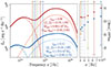 |
Fig. 2. Left panel: Spectral energy distribution (SED) of two selected MBHBs from our lightcone. The dashed, dotted and dash-dotted lines correspond to |


 (10)
(10)
where  is the limiting magnitude associated with the filter k = { u, g, r, i, z, y }. The values of
  for a single exposure and a 10 yr co-added image are presented in Table 1.
3.3. MBHB properties and LSST detectability
After outlining the procedure used to determine the EM emission of a MBHB, this section examines the LSST potential to detect MBHBs with observed orbital period ≤5 yr, i.e. suitable for effective periodic light curve analysis. In addition, we investigate their intrinsic and orbital properties.
In Fig. 3 we present the distribution of the apparent magnitudes for MBHBs with Pobs ≤ 5 yr. We note that the peak of all the distributions is at ∼30 − 35 mag, but for the sake of clarity we only present the distributions at < 27 mag. In all the panels, the vertical dotted (dashed) lines present the limiting magnitude of LSST for a single exposure (10 yr co-added), while the gray shaded areas indicate the regions beyond those thresholds. As we can see, the number of detectable sources in single-exposure mode is just a fraction (10−4 − 10−3) of the full population of MBHBs with Pobs ≤ 5 yr, being systematically smaller towards the reddest filters. This translates into ≈10−2 − 10−1 binaries per square degree potentially seen by LSST. It is interesting to notice that, thanks to its higher magnitude limit, the g-band is the one that features the most promising detectability with a total number of detections in a single exposure of ∼3 × 10⁻¹ deg−2. Similar trends are seen when we focus on the case of a magnitude limit based on 10 years of co-added images. In these cases, the total number of detected binaries can rise up to ≈1 − 10−2 deg−2. Despite the higher detection, the magnitude limit based on 10 years of co-added images does not allow multi-epoch variability studies. We note that any MBHB that is visible in a single exposure in any combination of the u, r, i, z, and y filters is also visible in g-LSST. This fact can be explained by examining any SED presented in Fig. 2. The spectrum drops quickly with decreasing ν, yet the g-filter sensitivity enables more detections if a MBHB magnitude is in the 23 − 24.5 range.
 |
Fig. 3. Distribution of MBHBs per deg2 as a function of magnitude. The vertical dotted and dashed lines correspond to the limiting magnitude of single and 10 yr co-added exposure modes, respectively. The dashed lines illustrate the cumulative probability functions of the full Pobs ≤ 5 yr MBHB population. In each panel, we show the number of MBHBs that are detectable in a single LSST exposure (Ndet, k, k ∈ { u, g, r, i, z, y }). |
In addition to magnitudes, it is particularly interesting to examine the properties of MBHBs with Pobs ≤ 5 yr that are detected in the single exposure mode of LSST. Specifically, we focus on the g-band, which is the one with the largest number of sources. Similar results are seen in different bands. The results are displayed in Fig. 4, where we present the distribution of the observed orbital period, total mass, eccentricity, mass ratio, and redshift. The detected population tends to occupy the higher-mass end of the distribution, with approximately 50% having a total mass MBHB > 107.5 M⊙. Furthermore, the detected systems are predominantly found at lower redshifts (zBHB ≲ 1.5) compared to the entire Pobs ≤ 5 yr MBHB population, which peaks around zBHB ≈ 2.5. As expected, the combination of high mass and low redshift is a key factor in producing a bright electromagnetic signal of an accreting MBH. Regarding the orbital properties, the systems feature a wide distribution of eccentricities. Cases with values lower than eBHB < 0.3 represent 25% of the population and correspond to the ones where the GW emission starts to dominate and circularise the system. 50% of the cases are concentrated at eBHB ∼ 0.6, a clear feature in our semi-analytical modelling that the MBHB systems are shrinking via gas hardening. Finally, the other 25% of the population features high eccentricity values associated with the cases where the stellar hardening dominates the MBHB evolution. Regarding the mass ratio, over half of the detected systems tend to favour the equal-mass configuration, with a median value  . This feature is just a natural consequence of the MBHB growth model included in L-Galaxies, which assumes preferential accretion on the secondary MBH, driving the MBHB towards qBHB = 1. Finally, detected systems feature longer orbital periods with respect to the general population distribution. In particular, our distribution features a median value of
  .
.
 |
Fig. 4. Distribution of the MBHB properties. From left to right: Observed orbital period (Pobs), redshift (zBHB), total mass (MBHB), eccentricity (eBHB), and mass ratio (qBHB). The grey distributions correspond to the full Pobs ≤ 5 yr MBHB population inside the lightcone. The red distributions correspond to the Pobs ≤ 5 yr MBHBs detectable in the g-LSST band. The solid lines represent the corresponding cumulative distributions. |
In summary, the results presented above indicate two fundamental and expected trends: variability studies with LSST will preferentially detect low-redshift (zBHB ≲ 1) and massive systems (MBHB ≳ 107 M⊙). Furthermore, the most common targeted systems are anticipated to be equal-mass binaries with moderate eccentricity, exhibiting modulation periods of approximately three years. This relatively long period constitutes a challenge since robust detection of variability over the existing red noise requires the observation of multiple (≳5) cycles (Vaughan et al. 2016). In this regard, we note that ≈65% of our detectable population will complete between two and three orbital cycles, while only ≈3% of our detectable MBHBs can complete more than five orbits over the course of ten years.
4. Variability modelling
Individually resolving MBHs in a binary system is a challenging task because of their close separation and short orbital periods. For this reason, variability studies to detect these objects at sub-pc scales have become a promising method. For instance, variability periodicities related to the accretion rate onto the binary may be directly detectable (see e.g. Artymowicz & Lubow 1996; Hayasaki et al. 2008; Graham et al. 2015b; Liu et al. 2015; Zheng et al. 2016). In this section, we present the methodology that we have adopted to create mock optical light curves for our MBHB population. Specifically, this is described first for a generic filter k, and then applied to our LSST case, i.e. k = {u, g, r, i, z, y}. We also emphasise that light curves are constructed for each MBHB in each LSST filter. However, when analysing the results in a specific band, we only consider the light curves of sources whose  meets the detectability criteria presented in Eq. (10).
4.1. Periodic variability: Hydrodynamic templates
The usual approach used in literature to build mock light curves of MBHBs consists of injecting a sinusoidal modulation in the MBHB emission (see e.g. Xin & Haiman 2024; Davis et al. 2024). Here, in contrast, we rely on the 3D hyper-Lagrangian resolution hydrodynamic simulations of accreting MBHBs presented in Cocchiararo et al. (2024). In this work the authors adopted the 3D meshless finite mass version of the code GIZMO (Hopkins 2015), with the addition of the particle splitting technique (see Franchini et al. 2022, for details) to increase the resolution inside the cavity carved by the binary. The authors modelled binaries embedded in a circumbinary disc coplanar with the binary orbit, with aspect ratio H/R = 0.1 and mass MD = 0.01 MB, where MB is the mass of the binary MB = 106 M⊙. The simulations include the contribution of the disc self-gravity (Roedig et al. 2011; Franchini et al. 2021, 2024). The thermodynamic evolution of the gas follows an adiabatic equation of state with index γ = 5/3, allowing the gas to change its temperature through shocks, PdV work, and black body radiation. The angular momentum transport is modelled using the α-viscosity prescription by Shakura & Sunyaev (1973). We exploit the optical emission produced by six different simulated MBHBs (hereafter ‘templates’, 𝒯) with a combination of eccentricities e𝒯 ∈ {0, 0.45, 0.9} and mass ratios q𝒯 ∈ {0.1, 0.7, 1}. In summary, each template includes the time evolution of the flux density emitted by a MBHB at z𝒯 = 1: ![Mathematical equation: $ \Phi^{\mathcal{T}_{i}}_{\nu}(\tau,\,z = 1)\,[{\mathrm{erg}\,\mathrm{cm}^{-2}\,\mathrm{s}^{-1}\,\mathrm{Hz}^{-1}}] $](/articles/aa/full_html/2026/03/aa57029-25/aa57029-25-eq22.gif) , where τ represents the simulation snapshot, and the subscript i = 1, 2, …, 6 denotes the specific template.
, where τ represents the simulation snapshot, and the subscript i = 1, 2, …, 6 denotes the specific template.
Each detectable source is matched with a template 𝒯i, following the decision tree illustrated in Table 2. For the sake of clarity, in the last column we present the number of LSST g-band detected sources associated with each template (Ndet, g). We want to notice that the assignment done for 𝒯1 and 𝒯5 can be considered too stretched because the relatively large difference between q𝒯 and the maximum q value allowed for the L-Galaxies MBHBs. Despite this, we do not expect any impact on our results due to the small number of binaries assigned to 𝒯5 templates and the small differences that we observed between 𝒯1 and 𝒯2 (see next sections). After matching a template 𝒯i with a MBHB, we adapt it to the source as follows:
Template properties, MBHB decision tree, and Ndet, g results.
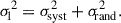
(i) Flux Adjustment – Our population of MBHBs covers abroad range of redshifts, while our templates are all located at z𝒯 = 1. As a consequence, when performing the template matching, the flux of 𝒯i would appear (dimmer) brighter compared to what is expected from a MBHB situated at redshift (lower) higher than z𝒯 = 1. In addition, brightness differences can also arise because our templates and MBHB population feature different accretion rates. To address the flux inconsistency resulting from variations in MBHB redshift, we adjust the template to match the redshift of the assigned MBHB (zBHB), i.e.  . On the other hand, the brightness differences between the template and the assigned binary caused by diverse accretion rates are addressed by defining the quantity
 (11)
(11)
where  corresponds to the average flux density per unit frequency at a given snapshot τ emitted by the template 𝒯i inside a given k filter (see Section 3.2). The quantity
  corresponds to the median average flux density computed over all the snapshots. Taking into account the ℱk(τ, zBHB) quantity and the redshift correction associated with 𝒯i, we build the MBHB light curve as
![Mathematical equation: $$ \begin{aligned} \begin{split} m_{k}(\tau )&= m^\mathrm{BHB}_{k} + \Delta m^{\mathcal{T} _{i}}_{k}(\tau )\\ \ &= m^\mathrm{BHB}_{k}\,{-}\,2.5 \log _{10}\big [\mathcal{F} _{k}(\tau , \, z = z_{\rm BHB}) \big ] \,, \end{split} \end{aligned} $$](/articles/aa/full_html/2026/03/aa57029-25/aa57029-25-eq27.gif) (12)
(12)
where  is the magnitude of the simulated L-Galaxies MBHB (computed as outlined in Section 3.2) and
  its associated variability. In Fig. 5, we show several examples of
  as a function of the MBHB orbits. As shown, the fluctuations can be small (≲0.5 mag) for the case of circular binaries while they reach up to ∼1 mag in the case of non-negligible eccentricities (see Cocchiararo et al. 2024, for further information).
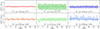 |
Fig. 5. Visualisation of the g-band variability prescribed by our templates, Δmg𝒯(z = 1), as a function of the last 30 orbits. Each panel represents a different hydrodynamical simulation from Cocchiararo et al. (2024). The template parameters (e𝒯, q𝒯) are shown in each panel. |
(ii) Time conversion – Each template includes only the snapshots taken from the hydrodynamics simulations after the system has reached a stable configuration and a quasi steady-state accretion regime (see Cocchiararo et al. 2024, for details) for details. The snapshots are spaced such that ten of them correspond to one binary orbit of the simulated MBHB. Using this relation and the orbital period of each selected binary, we convert snapshot indices into time as
 (13)
(13)
where the index ι runs over the NS snapshots used in each template, depending on the specific simulation. In the case 𝒯1, NS = 2500. For the template 𝒯2, NS = 2000. In the case 𝒯3, NS = 1000. Lastly, NS = 3000 for the other templates.
(iii) Cadence adjustment – LSST is expected to have an observing cadence of approximately 𝒞LSST ≈ 2 − 4 days (Ivezić et al. 2019). However, the cadence of hydrodynamical simulation snapshots is much lower, around 90 days, which limits our ability to create accurate LSST mock light curves. To address this limitation, we set a fixed LSST cadence of 𝒞 = 3 days and linearly interpolate our template points to match this observation rate. This approach allows us to generate an evenly spaced time series that better simulates LSST observations. The resulting light curve ends up having a duration that is much longer than the LSST mission itself. Thus, to customise it to the LSST observing time, we extract ten years of contiguous data from the full time series, by selecting a random starting time t0. For clarity, we display the tailoring of the 𝒯3 data to a selected MBHB in Fig. 6. The red dots in the middle panel show the g-band template data once the flux adjustments and time conversion are applied: the values are set to oscillate around  . For clarity, we do not illustrate their linear interpolation.
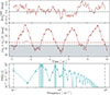 |
Fig. 6. Example of light curve construction in the LSST g-band. The selected source features MBHB ≃ 4.91 × 10⁷ M⊙, zBHB ≃ 1.95, Pobs ≃ 2.45 yr, eBHB = 0.6, and qBHB ≃ 0.7. First panel: Random DRW realisation associated with the MBHB. Second panel: Realisation of a single mg(t) light curve. The dots represent the tailored 𝒯3 data points. The solid line implements the DRW shift from the first panel, plus the manipulations presented in Sections 4.1–4.4. Third panel: Periodogram analysis of mg(t). The vertical green dashed lines represent the Keplerian frequency and the second and third harmonics, while the corresponding shaded regions represent the frequency bin width. Finally, the vertical thick shaded grey lines mark the periodogram fmin and fmax values. |
4.2. Intrinsic variability: The damped random walk
The variable photometry discussed in the previous section represents an idealised scenario in which no noise effects influence the time evolution of the curve. To create a more realistic dataset, we add stochastic optical variability according to the damped random walk (DRW) model, i.e. the standard model used to describe the optical variability of quasars (Kelly et al. 2009; Kozłowski et al. 2010; MacLeod et al. 2010). We emphasise that this model is typically used to analyse the intrinsic variability of individual accreting objects. Nevertheless, we assume its validity for the MBHBs in our study, which simplifies our description. To implement the DRW, we implement and solve the following stochastic differential equation (Brockwell & Davis 2016):
 (14)
(14)
The equation gives the amplitude of the magnitude variations due to the DRW model (after fixing ⟨m⟩ = 0). Here m(t) is the light curve of the target source and ϵ(t) is a white noise with zero mean and unit variance, which we assume to be Gaussian (as in Kelly et al. 2009). The quantities τ and σ are instead related to the properties of the central object (in our case, a MBHB). The former is referred to as relaxation timescale, and quantifies how the emission is damped over large timescales. The latter is instead the standard deviation of the magnitude distribution, and it is related to the MBHB via the structure function term, SF(Δt).
Over short timescales (Δt ≪ τ) the DRW is an ordinary random walk. Over long timescales (Δt ≫ τ), SF asymptotically tends to
![Mathematical equation: $$ \begin{aligned} \mathrm{SF}_{\infty } = \sqrt{2}\sigma \, [\mathrm{mag}]. \end{aligned} $$](/articles/aa/full_html/2026/03/aa57029-25/aa57029-25-eq34.gif) (15)
(15)
We compute both τ and SF∞ following MacLeod et al. (2010):
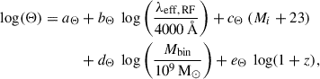 (16)
(16)
where Θ refers either to SF∞ [mag] or to τ [days]. The array of parameters (aΘ, bΘ, cΘ, dΘ, eΘ) is taken from Table 1 of MacLeod et al. 2010: we set (−0.51, −0.479, 0.131, 0.18, 0.0) for Θ = SF∞ and (2.4, 0.17, 0.03, 0.21, 0.0) for Θ = τ. The variable λeff, RF refers to the effective rest-frame wavelength of each filter, i.e. λeff, RF = λeff (1 + z)−1, with z being the MBHB redshift. Finally, Mi corresponds to the absolute magnitude of the object in the SDSS i-band (computed as described in Section 3.2).
Once all the parameters associated with the DRW are determined, we use Eq. (14) to compute the amplitude of the magnitude variation due to the DRW at each time step of our light curve,  . For clarity, the top panel of Fig. 6 displays a 10 yr realisation of this stochastic process for a single MBHB in the g-band. As shown, the amplitude of this DRW can easily exceed 0.3 mag. Therefore, by considering the DRW, the light curve of a given MBHB can now be described by the expression
 (17)
(17)
4.3. Photometric errors
To make the light curves more realistic, we also take into account the observational uncertainty in each observing point of our light curve. To this end, we estimate the photometric error of a single LSST exposure, hereafter σ1, as defined in Ivezić et al. (2019):
 (18)
(18)
The constant σsyst indicates a systematic error, which we set to the estimated upper limit of 0.005 mag. On the other hand, σrand is related to the source brightness by
![Mathematical equation: $$ \begin{aligned} \sigma ^{2}_{\!\mathrm {rand}} = (0.04\,{-}\,\gamma ) \,x + \gamma \,x^{2} \, [\mathrm{mag^{2}}], \end{aligned} $$](/articles/aa/full_html/2026/03/aa57029-25/aa57029-25-eq39.gif) (19)
(19)
with log10x = 0.4 (m − m5). The quantity m5 denotes the 5σ depth in a given band, taken from Table 3.2 of Ivezić et al. (2019). As a result, the uncertainty associated with a point mk(tj) is largest for the faintest points.
To account for the photometric uncertainties described earlier, each data point mk(t) in the light curve (see Eq. (17)) is resampled. Specifically, we draw a random value from a Gaussian distribution centred on the flux fν, k(t) associated with mk(t) with a variance σ1, flux = σ1 × fν, k(t) × ln (10)/2.5 where σ1 is defined in Eq. (18). The sampled flux is then converted into a magnitude, which reflects the photometric errors applied to the original measurement. To aid in the visualisation of the typical shape of our realistic light curves, we present a single MBHB light curve realisation in the middle panel of Fig. 6, as seen by the LSST g-band. As illustrated, the overall shape of this final light curve resembles that of the tailored template data. However, some wiggles and jumps appear due to the effects of DRW. Moreover, the observational uncertainties are largest where m → m5.
4.4. LSST observation patterns
Although the nominal cadence time of LSST is approximately three days, not all filters are used to observe each pointing on a given night. Instead, LSST employs a filter cycling strategy, where each pointing is simultaneously observed using a pair of filters following a specific pattern (Lochner et al. 2022):
 (20)
(20)
We also implement this strategy on constructing our light curves, generating separate time series for each filter k. By incorporating this observing strategy, the final observing cadence of an object in a specific filter is no longer evenly spaced. Furthermore, the number of observations of a given object in each filter decreases to ∼30% of the total number of LSST visits.
4.5. Periodogram analysis
In this section, we aim to assess the successful identification of variable MBHBs using LSST. Specifically, we evaluate how often a light curve from a MBHB can be confidently identified as originating from a binary system (success rate, 𝒮ℛ). Additionally, we estimate the false alarm probability (FAP) associated with our MBHB signals. Following the previous sections, the results are only explored for the g-band as it is the one that provides the largest number of detected sources.
PSD construction – The first step required to characterise the 𝒮ℛ of our MBHB population consists of analysing the power spectral density (PSD) of the observed light curves. We calculate the PSD using the Lomb (1976) procedure, as it allows us to construct the periodogram of a signal with uneven time sampling. Specifically, given a MBHB light curve mk(tj), (see Eq. (17)), our algorithm generates its PSD as a function of an array of frequencies, PSD(f), which spans from fmin = 0.1 yr−1 (assuming a 10 yr duration for the LSST survey) to fmax = 0.5 /2π𝒞 yr−1 (Nyquist frequency), in steps of fmin. In the bottom panel of Fig. 6, we display the results for a single MBHB light curve in the g-band.
Success rate (𝒮ℛ) – Once the PSD(f) is computed, we identify its maximum (hereafter, ‘intensity’) and determine its corresponding frequency bin, Δfj. We then assume that the MBHB has been ‘correctly identified’ whenever it satisfies the condition
 (21)
(21)
where fk is the MBHB Keplerian frequency. In Fig. 6, we display a correct identification, where the PSD maximum and the MBHB Keplerian frequency are in the same frequency bin. To ensure strong statistical significance of the previous methodology and to avoid relying on particularly lucky configurations in the light curve construction2, we evaluate Eq. (21) over a total of NR = 105 light curve realisations for each MBHB. For each of these realisations, the starting point t0 of the hydrodynamical signal is extracted randomly and matched with an independent realisation of DRW and photometric errors. As a result, for a given MBHB, its 𝒮ℛ is defined as
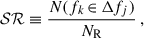 (22)
(22)
where N(fk ∈ Δfj) corresponds to the number of realisations which satisfy Eq. (21).
False alarm probability (FAP) – To determine the FAP of our light curves, we need to assess the likelihood that a detected signal corresponds to just random noise, rather than a genuine MBHB signature. To this end, we examine the DRW of Section 4.2 by characterising the distribution of SF∞ and τ values associated with our detectable MBHBs3. We thus generate a family of NDRW = 106 noise realisations,
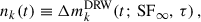 (23)
(23)
where SF∞ and τ are sampled from their corresponding distributions. Then, we compute the PSD associated with these noise realisations following the Lomb (1976) procedure. This yields a distribution of NDRW PSD values in each of the frequency bins Δfj, sampled as in the 𝒮ℛ case. We now define Ii ≡ PSD(fi) as the signal-PSD intensity in the i-th frequency bin and pj(I) as the distribution of the NDRW intensities in a given frequency bin j. Consider a binary with a maximum intensity  in the i-th bin. The probability that this maximum is generated by pure noise is
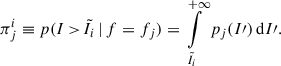 (24)
(24)
Interestingly, the periodogram associated with the MBHB may feature some other spikes at frequencies associated with the Keplerian harmonics of the source. This is clearly the case in the last panel of Fig. 6, where three clear peaks appear at fk (j = 4), 2fk (j = 8), and even 3fk (j = 12). Hence, we define a FAP accounting for correlated intensities at a frequency fi and 2fi as4
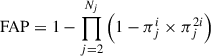 (25)
(25)
where πji and πj2i are computed according to Eq. (24). We note that the frequency bin j = 1 is excluded from Eq. (25) for two reasons. First, a maximum for fk = 0.1 yr−1 would correspond to a binary with an orbital period greater than 5 yr, which would be incompatible with the sources in our analysis. Second, the first frequency bin of a periodogram is known to have an excess of power (Bloomfield 1976; Harris 1978). We adopt an approach similar to that of the 𝒮ℛ case, to ensure robust statistical significance of the previous methodology and to prevent reliance on particularly lucky configurations in the light curve construction. We thus evaluate the FAP of Eq. (25) over a total of NR = 105 light curve realisations for each MBHB. These realisations are generated following the procedure outlined for the 𝒮ℛ case.
5. Detectability through variability studies
In this section, we present the results regarding the success rate and the FAP. We emphasise that these results are based solely on the sources detected in the g-band, as they represent the largest sample. The results based on other filters show similar trends.
We present the predictions for the success rates in Fig. 7, separated into six groups according to the adopted template 𝒯. Circular binaries feature mostly 𝒮ℛ ≲ 40%. Conversely, MBHBs associated with eccentric systems feature a trend of higher 𝒮ℛ towards higher eccentricities. For example, the cases associated with e𝒯 = 0.45 feature 𝒮ℛ ≈ 50% while those with e𝒯 = 0.9 have 𝒮ℛ ≳ 60%. This trend can be explained by the fact that the signal of an eccentric MBHB is dominated by its Keplerian frequency, or some of its harmonics (see Kelley et al. 2019, as an example). This causes the PSD associated with the light curve to show a clear peak at the MBHB fk, easily identifiable by our analysis. In addition, the low success rate for non-eccentric systems can also be explained by comparing the templates of Fig. 5 with a standard DRW realisation shown in Fig. 6. As shown, the typical magnitude amplitude of the latter is ∼0.2, which is roughly of the same order of magnitude of the fluctuations seen in the circular templates (𝒯1 and 𝒯2). These similarities result in the periodogram having difficulties identifying the MBHB Keplerian frequency. Finally, in all the distributions shown in Fig. 7, there is a tail of low 𝒮ℛ, independently of the mass ratio and eccentricity of the template. We have checked that these cases correspond either to systems with the longest orbital periods or to faint objects, with part of their light curve falling below the LSST sensitivity. Having a few or incomplete orbital periods causes the periodogram methodology to be less effective at properly reconstructing the Fourier components. Finally, we have also observed that at fixed eccentricity the detections tend to prefer systems with more unequal mass ratios. For example, in the case of circular binaries, 𝒮ℛ ≲ 20% for q𝒯 = 1, while 𝒮ℛ ≲ 30% for q𝒯 = 0.1.
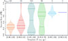 |
Fig. 7. Success rate of detecting MBHBs via variability studies in the g-band of LSST. The results are presented as a function of the MBHB properties, grouped according to the associated template. We used a total NR = 105 light curves for each MBHB, which in turn yielded a single 𝒮ℛ value per object. Each distribution thus contains Ndet, g entries. The coloured regions represent the total distribution while the horizontal segments locate the 25th, 50th, and 75th quantiles of each distribution. |
The FAP results are shown in Fig. 8. As we did in Fig. 7, we have separated our MBHBs according to their associated template. Interestingly, eccentric MBHBs (associated with 𝒯3 and 𝒯4) show a FAP value that can be as low as ≈10−8. Conversely, circular MBHBs (associated with 𝒯1 and 𝒯2) feature much larger FAP values, with median values as large as ∼0.6. The higher FAP values are due to two factors. First, for circular binaries, the Keplerian frequency is less dominant in the light curve, and the highest peak in the power spectral density (PSD) may be caused by noise rather than by a true signal. This noise peak could be similar in strength to what is expected from a pure DRW process (see Vaughan 2009, for details). Second, the second PSD peak used in the FAP analysis might not be related to the MBHB periodicity at all. It could simply be a random fluctuation in the PSD, independent of any real signal. As shown in Fig. 5, eccentric systems are less affected by these two issues as their PSD features are more pronounced and their multiple peaks are correlated. Finally, as seen in the success rate analysis, the FAP also depends on the mass ratio. Specifically, at fixed eccentricity, FAP values are lower for more unequal-mass systems. For example, systems with e𝒯 = 0.9 have FAPs of ∼10−3 for q𝒯 = 0.1, increasing to ∼10−2 for q𝒯 = 1. At the bottom of Fig. 8, we display the percentage of realisations where the computed FAP is equal to zero: this event occurs, as we constructed our noise distribution with a finite number of realisations of the DRW. If the PSD peak produced by a binary surpasses the highest value achieved by all the DRW realisations, then the integral in Eq. (24) is zero. In the case of 𝒯3, this is a systematic feature of our systems, whose signal can be unambiguously identified as a MBHB light curve.
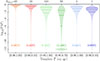 |
Fig. 8. False alarm probability (FAP) in variability studies in g-LSST. The results are presented as a function of the MBHB properties, grouped according to the used template. We used a total NR = 105 light curves for each MBHB, and each distribution encloses a total of Ndet, g × 105 entries. The coloured regions represent the total distribution while the horizontal segments locate the 25th, 50th, and 75th quantiles of each distribution. In all the distributions, the peak at FAP = 10−12 corresponds to cases where we find FAP values equal to 0. |
6. Caveats
Our model relies on several simplifying assumptions, which can affect our inference and our results:
-
(a)
Underlying SAM assumptions – The results presented here are based on a population of MBHBs generated by the L-Galaxies SAM, which relies on specific assumptions regarding the formation and evolution of MBHs and MBHBs. In the context of this work, changing the set of underlying assumptions or physical models can yield to variations in the population, such as a change in the number of objects, as well as in the distributions in mass, mass ratio, semi-major axis, and eccentricity.
-
(b)
Lightcone construction strategy – To create the wide sky area covered by our lightcone, we require a large number of Millennium-II box replications (see the methodology presented in Izquierdo-Villalba et al. 2019). Thus, our catalogue of detectable MBHBs can contain some ‘duplicated’ sources.
-
(c)
Construction of the MBHB SEDs – A crucial step in our study is estimating the MBHB average electromagnetic emission, which depends on the assumed SED. In particular, we modelled it as the independent combination of two mini-discs and a circumbinary disc. However, we neglected any contribution from gas streams penetrating inside the cavity carved by the binary. This causes a clear dip (or notch) to appear in the MBHB spectrum (see Fig. 2). In fact, Cocchiararo et al. (2024) recently demonstrated that gas streams around the MBHB can contribute significantly to the electromagnetic emission, accounting for ∼20% of the system total luminosity. We are thus selecting the brightest and most massive sources, which complete few orbital cycles in LSST. Implementing the stream emission would increase the number of detectable sources, with a crucial effect on dimmer, lower-mass systems with a larger number of orbital cycles. Our description of the active MBHB population is thus seen as a lower limit for their LSST detectability.
-
(d)
Template assignment strategy – The decision tree presented in Table 2 couples each MBHB with one hydrodynamic prescription 𝒯i, to estimate its variable emission. Here, the qBHB = 0.8 threshold is adopted to split between templates, as it is the mean value of the g-band detected population. However, this choice becomes rather stretched whenever | qBHB − 0.8 | is large. To improve our assignment accuracy, a denser parameter space sampling from the hydrodynamic simulations is required.
-
(e)
Systems in the ADAF accretion mode – Given the lack of an accurate ADAF model for MBHB systems, we have decided to exclude from our analysis those systems whose accretion rates are compatible with this accretion mode. This exclusion implies that we are neglecting ∼40% of the accreting MBHB population with an observed period Pobs ≤ 5 yr, which could be potentially visible in LSST. We expect these objects to be dimmer than the TD + TD population, and the fraction of detectable objects being neglected to be small. It is also possible that our current catalogue may be biased towards equal mass systems, due to our preferential accretion strategy (see Eq. (1)).
-
(f)
Stochastic optical variability of MBHBs – The DRW model used was originally designed and calibrated to characterise the optical variability of individual AGNs, not binary systems. Given the separation of our objects, it is reasonable to assume that their gas accretion processes could be correlated. However, relying on a single DRW to represent the intrinsic variability of the pair might be an oversimplification.
-
(g)
Processes leading to a variable light curve – The six hydrodynamical simulations used to assign variable light curves naturally account for the changes and fluctuations in the behaviour of the gas and fluid dynamics around the two MBHs in the binary system (hydrodynamic variability). However, other effects can also induce periodic variations in the emission from MBHBs. Among these, we can find the Doppler boost (D’Orazio et al. 2015), which leads to an increase and a decrease of the MBHB luminosity due to the relativistic motion between the two orbiting MBHs or binary self-lensing (D’Orazio & Di Stefano 2018), that can periodically magnify the flux directed towards the observer. As shown by Kelley et al. (2021), about 𝒪(101 − 102) self-lensing binaries could be discovered using LSST, with a typical mass that is comparable to that of our detectable sources. We plan to implement a more realistic modelling of our light curves in a future work. In this work, we have neglected any of these additional processes. Incorporating them could introduce distinctive features to the periodograms, potentially enhancing our ability to identify and study MBHBs more effectively. We refer to the binlite code presented by D’Orazio et al. (2024), which implements these features for equal-mass systems in a wide range of orbital eccentricities and generates mock MBHB light curves. In contrast to binlite, which relies on results obtain from 2D fixed-orbit numerical hydrodynamical simulations and infers luminosity variations from the accretion rate, our model is based on fully 3D solutions. This allows us to compute the temperature of the gas assuming an optically thick disc and obtain the luminosity directly from the local black body emission of each pixel of the simulated domain. Moreover, 3D codes can track the evolution of the disc aspect ratio, which determines the amount of gas accreted onto the binary.
-
(h)
Use of the periodogram – Our detection method relies on the Lomb-Scargle periodogram, which is known to be sub-optimal for non-sinusoidal signals (Lin et al. 2026). Our choice of using a fixed-frequency bin array is the most naïve and uses the lowest number of frequencies. A larger number of bins would introduce correlations between the resulting PSD(fj) values, yet it would lead to a better estimate of the signal FAPs. We refer to Section 7.4.2 of VanderPlas (2018) for details. According to the author, our estimates (computed using Equation (25)) are likely underestimating the FAP by a factor 𝒪(10). We plan to explore more sophisticated methodologies exploiting Gaussian processes in a future work (Cocchiararo et al. in prep.).
-
(i)
Host galaxy light and dust – Our work neglects the contribution of the host galaxy light and the potential attenuation caused by dust particles along the line of sight. The former enters the detected emission, and can rival the MBHB periodic signal. This, in turn, would make the identification more challenging and with higher FAPs. We are also ignoring the attenuation exerted by dust on the periodic light curves. The attenuation is stronger at shorter wavelengths, hence the u− and g−bands may be the most affected (Salim & Narayanan 2020).
7. Conclusions
In this work, we explored the potential of using the LSST survey to perform variability analyses aimed at identifying MBHBs. To do so, we used a population of simulated MBHBs extracted from a lightcone generated by the L-Galaxies SAM. Among this population, we focused exclusively on systems with observed orbital periods suitable for effective periodic light curve analysis. Specifically, we limited our study to objects with observed orbital periods Pobs ≤ 5 yr after considering the LSST ten-year survey duration and the requirement to observe at least two complete emission cycles within that time.
To generate mock optical light curves for such a targeted MBHB population, we followed a systematic procedure. First, we calculated the system average magnitude in each LSST filter by constructing self-consistent SEDs for each MBHB. This accounts for the accretion history of the binary and the modelling of the resulting emission generated by the circumbinary disc as well as the two mini-discs surrounding each MBH. Next, we incorporated variability into the light curves by using six 3D hydrodynamic simulations of accreting MBHBs with different eccentricities and mass ratios as templates. This step involved applying flux adjustments, time conversions, and modifying the observation cadence to adapt the hydrodynamical outputs to our specific MBHB systems and the observational specifications of the LSST survey. Finally, to produce more realistic light curves, we incorporated stochastic variability using a damped random walk model (DRW) and added photometric errors consistent with LSST observational uncertainties. These light curves were processed with a periodogram analysis, to determine the successful recovery of variable MBHBs and the associated false alarm probability. We hereby summarise our main results as follows:
-
(1)
The number of MBHBs with Pobs ≤ 5 yr that are detectable in single LSST exposure mode corresponds to a fraction 10−4 − 10−3 of the whole Pobs ≤ 5 yr MBHB population, depending on the LSST filter. This corresponds to 𝒪(10−1)−𝒪(10−2) binaries per square degree. This result is explained by the low magnitude of MBHBs, which is both a result of their intrinsic luminosity and distance from the observer. Thanks to its deeper magnitude limit, the g-band is the one that features the most promising detectability with a total number of detections in a single exposure of ∼3 × 10⁻¹deg−2.
-
(2)
Detected MBHBs with Pobs ≤ 5 yr are placed at zBHB ≲ 1.5 and favour higher masses than average. In fact, approximately 50% of the population has a total mass MBHB > 107.5 M⊙. The systems feature a wide distribution of eccentricities, but a large majority have eBHB ≳ 0.6, a clear feature in our semi-analytical modelling of systems shrinking via gas hardening. Regarding the mass ratio, over half of the detected systems tend to favour the equal-mass configuration, with a median value
 .
. -
(3)
LSST variability studies detect more easily MBHBs with high eccentricities. While circular systems have a recovery success rate ≤40%, eccentric MBHBs (eBHB ≳ 0.6) are successfully detected in over 50% of cases. Additionally, for a fixed eccentricity the detections tend to prefer systems with lower mass ratios.
-
(4)
The false alarm probability (FAP) in LSST variability studies shows trends similar to the success rate case. Highly eccentric systems feature a low-FAP tail (up to ∼10−8) that circular ones do not display (≳10−2). The FAP also depends on the mass ratio, and is smaller in systems with lower mass ratios.
In summary, the results presented in this work represent an initial effort to understand and characterise the population of MBHBs that could potentially be detected through LSST variability studies. Our findings suggest that LSST has the potential to identify variable MBHBs and reveal a new population of sources. However, there are some limitations to consider. These include simplified assumptions in our SED modelling and the omission of other processes that can produce variability patterns. In a future follow-up paper, we plan to address these caveats in detail to better assess the full potential of variability studies with LSST data.
Acknowledgments
We thank the B-Massive group at Milano-Bicocca University for useful discussions and comments. A.C. thanks Lorenzo Bertassi for his friendship and comments to this work. D.I.V and A.S. acknowledge the financial support provided under the European Union’s H2020 ERC Consolidator Grant “Binary Massive Black Hole Astrophysics” (B Massive, Grant Agreement: 818691) and the European Union Advanced Grant “PINGU” (Grant Agreement: 101142079). AL acknowledges support by the PRIN MUR “2022935STW” funded by European Union-Next Generation EU, Missione 4 Componente 2, CUP C53D23000950006. D.S. acknowledges support by the Fondazione ICSC, Spoke 3 Astrophysics and Cosmos Observations. National Recovery and Resilience Plan (Piano Nazionale di Ripresa e Resilienza, PNRR) Project ID CN_00000013 “Italian Research Center on High-Performance Computing, Big Data and Quantum Computing” funded by MUR Missione 4 Componente 2 Investimento 1.4: Potenziamento strutture di ricerca e creazione di “campioni nazionali di R&S (M4C2-19)” – Next Generation EU (NGEU). S.B. acknowledges support from the Spanish Ministerio de Ciencia e Innovación through project PID2021-124243NB-C21.
References
- Aird, J., Coil, A. L., Georgakakis, A., et al. 2015, MNRAS, 451, 1892 [Google Scholar]
- Angulo, R. E., & White, S. D. M. 2010, MNRAS, 405, 143 [NASA ADS] [Google Scholar]
- Artymowicz, P., & Lubow, S. H. 1994, ApJ, 421, 651 [Google Scholar]
- Artymowicz, P., & Lubow, S. H. 1996, ApJ, 467, L77 [NASA ADS] [CrossRef] [Google Scholar]
- Barausse, E., & Rezzolla, L. 2009, ApJ, 704, L40 [NASA ADS] [CrossRef] [Google Scholar]
- Begelman, M. C., Blandford, R. D., & Rees, M. J. 1980, Nature, 287, 307 [Google Scholar]
- Bertassi, L., Sottocorno, E., Rigamonti, F., et al. 2025, A&A, 702, A165 [NASA ADS] [CrossRef] [EDP Sciences] [Google Scholar]
- Biava, N., Colpi, M., Capelo, P. R., et al. 2019, MNRAS, 487, 4985 [Google Scholar]
- Bloomfield, P. 1976, Fourier Analysis of Time Series: An Introduction (Wiley) [Google Scholar]
- Bonetti, M., Rasskazov, A., Sesana, A., et al. 2020, MNRAS, 493, L114 [Google Scholar]
- Bonoli, S., Marulli, F., Springel, V., et al. 2009, MNRAS, 396, 423 [NASA ADS] [CrossRef] [Google Scholar]
- Boylan-Kolchin, M., Ma, C.-P., & Quataert, E. 2006, MNRAS, 369, 1081 [CrossRef] [Google Scholar]
- Brockwell, P. J., & Davis, R. A. 2016, Introduction to Time Series and Forecasting (Springer) [Google Scholar]
- Capelo, P. R., Volonteri, M., Dotti, M., et al. 2015, MNRAS, 447, 2123 [NASA ADS] [CrossRef] [Google Scholar]
- Charisi, M., Bartos, I., Haiman, Z., et al. 2016, MNRAS, 463, 2145 [Google Scholar]
- Charisi, M., Haiman, Z., Schiminovich, D., & D’Orazio, D. J. 2018, MNRAS, 476, 4617 [Google Scholar]
- Ciurlo, A., Mannucci, F., Yeh, S., et al. 2023, A&A, 671, L4 [NASA ADS] [CrossRef] [EDP Sciences] [Google Scholar]
- Cocchiararo, F., Franchini, A., Lupi, A., & Sesana, A. 2024, A&A, 691, A250 [NASA ADS] [CrossRef] [EDP Sciences] [Google Scholar]
- Comerford, J. M., & Greene, J. E. 2014, ApJ, 789, 112 [NASA ADS] [CrossRef] [Google Scholar]
- Comerford, J. M., Gerke, B. F., Stern, D., et al. 2012, ApJ, 753, 42 [Google Scholar]
- Cuadra, J., Armitage, P. J., Alexander, R. D., & Begelman, M. C. 2009, MNRAS, 393, 1423 [Google Scholar]
- Davis, M. C., Grace, K. E., Trump, J. R., et al. 2024, ApJ, 965, 34 [Google Scholar]
- De Rosa, A., Vignali, C., Bogdanović, T., et al. 2019, New Astron. Rev., 86, 101525 [Google Scholar]
- Dekany, R., Smith, R. M., Riddle, R., et al. 2020, PASP, 132, 038001 [NASA ADS] [CrossRef] [Google Scholar]
- Di Matteo, T., Springel, V., & Hernquist, L. 2005, Nature, 433, 604 [NASA ADS] [CrossRef] [Google Scholar]
- D’Orazio, D. J., & Charisi, M. 2023, ArXiv e-prints [arXiv:2310.16896] [Google Scholar]
- D’Orazio, D. J., & Di Stefano, R. 2018, MNRAS, 474, 2975 [CrossRef] [Google Scholar]
- D’Orazio, D. J., & Loeb, A. 2018, ApJ, 863, 185 [Google Scholar]
- D’Orazio, D. J., Haiman, Z., & MacFadyen, A. 2013, MNRAS, 436, 2997 [Google Scholar]
- D’Orazio, D. J., Haiman, Z., & Schiminovich, D. 2015, Nature, 525, 351 [Google Scholar]
- D’Orazio, D. J., Haiman, Z., Duffell, P., MacFadyen, A., & Farris, B. 2016, MNRAS, 459, 2379 [Google Scholar]
- D’Orazio, D. J., Duffell, P. C., & Tiede, C. 2024, ApJ, 977, 244 [Google Scholar]
- Dotti, M., Colpi, M., Haardt, F., & Mayer, L. 2007, MNRAS, 379, 956 [NASA ADS] [CrossRef] [Google Scholar]
- Dotti, M., Rigamonti, F., Rinaldi, S., et al. 2023, A&A, 680, A69 [NASA ADS] [CrossRef] [EDP Sciences] [Google Scholar]
- Duffell, P. C., D’Orazio, D., Derdzinski, A., et al. 2020, ApJ, 901, 25 [NASA ADS] [CrossRef] [Google Scholar]
- Escala, A., Larson, R. B., Coppi, P. S., & Mardones, D. 2004, ApJ, 607, 765 [NASA ADS] [CrossRef] [Google Scholar]
- Escala, A., Larson, R. B., Coppi, P. S., & Mardones, D. 2005, ApJ, 630, 152 [Google Scholar]
- Farris, B. D., Duffell, P., MacFadyen, A. I., & Haiman, Z. 2014, ApJ, 783, 134 [NASA ADS] [CrossRef] [Google Scholar]
- Fontecilla, C., Chen, X., & Cuadra, J. 2017, MNRAS, 468, L50 [Google Scholar]
- Franchini, A., Sesana, A., & Dotti, M. 2021, MNRAS, 507, 1458 [NASA ADS] [Google Scholar]
- Franchini, A., Lupi, A., & Sesana, A. 2022, ApJ, 929, L13 [NASA ADS] [CrossRef] [Google Scholar]
- Franchini, A., Lupi, A., Sesana, A., & Haiman, Z. 2023, MNRAS, 522, 1569 [NASA ADS] [CrossRef] [Google Scholar]
- Franchini, A., Bonetti, M., Lupi, A., & Sesana, A. 2024, A&A, 686, A288 [NASA ADS] [CrossRef] [EDP Sciences] [Google Scholar]
- Ge, J., Lu, Y., Yan, C., & Liu, J. 2024, A&A, 687, A57 [NASA ADS] [CrossRef] [EDP Sciences] [Google Scholar]
- Genzel, R., & Townes, C. H. 1987, ARA&A, 25, 377 [CrossRef] [Google Scholar]
- Goicovic, F. G., Cuadra, J., Sesana, A., et al. 2016, MNRAS, 455, 1989 [NASA ADS] [CrossRef] [Google Scholar]
- Graham, M. J., Djorgovski, S. G., Stern, D., et al. 2015a, Nature, 518, 74 [Google Scholar]
- Graham, M. J., Djorgovski, S. G., Stern, D., et al. 2015b, MNRAS, 453, 1562 [Google Scholar]
- Haehnelt, M. G., & Rees, M. J. 1993, MNRAS, 263, 168 [Google Scholar]
- Haiman, Z., Kocsis, B., & Menou, K. 2009, ApJ, 700, 1952 [CrossRef] [Google Scholar]
- Haring, N., & Rix, H.-W. 2004, ApJ, 604, L89 [NASA ADS] [CrossRef] [Google Scholar]
- Harris, F. J. 1978, IEEE Proc., 66, 51 [NASA ADS] [CrossRef] [Google Scholar]
- Hayasaki, K., Mineshige, S., & Sudou, H. 2007, PASJ, 59, 427 [NASA ADS] [Google Scholar]
- Hayasaki, K., Mineshige, S., & Ho, L. C. 2008, ApJ, 682, 1134 [NASA ADS] [CrossRef] [Google Scholar]
- Henriques, B. M. B., White, S. D. M., Thomas, P. A., et al. 2015, MNRAS, 451, 2663 [Google Scholar]
- Hopkins, P. F. 2015, MNRAS, 450, 53 [Google Scholar]
- Hopkins, P. F., & Hernquist, L. 2009, ApJ, 698, 1550 [NASA ADS] [CrossRef] [Google Scholar]
- Hopkins, P. F., & Quataert, E. 2010, MNRAS, 407, 1529 [Google Scholar]
- Hopkins, P. F., Hernquist, L., Martini, P., et al. 2005, ApJ, 625, L71 [Google Scholar]
- Hopkins, P. F., Hernquist, L., Cox, T. J., et al. 2006, ApJ, 639, 700 [NASA ADS] [CrossRef] [Google Scholar]
- Hopkins, P. F., Richards, G. T., & Hernquist, L. 2007, ApJ, 654, 731 [Google Scholar]
- Hwang, H.-C., Shen, Y., Zakamska, N., & Liu, X. 2020, ApJ, 888, 73 [NASA ADS] [CrossRef] [Google Scholar]
- Ivanov, P. B., Papaloizou, J. C. B., & Polnarev, A. G. 1999, MNRAS, 307, 79 [Google Scholar]
- Ivezić, Ž., Kahn, S. M., Tyson, J. A., et al. 2019, ApJ, 873, 111 [Google Scholar]
- Izquierdo-Villalba, D., Angulo, R. E., Orsi, A., et al. 2019, A&A, 631, A82 [NASA ADS] [CrossRef] [EDP Sciences] [Google Scholar]
- Izquierdo-Villalba, D., Bonoli, S., Dotti, M., et al. 2020, MNRAS, 495, 4681 [NASA ADS] [CrossRef] [Google Scholar]
- Izquierdo-Villalba, D., Sesana, A., Bonoli, S., & Colpi, M. 2022, MNRAS, 509, 3488 [Google Scholar]
- Izquierdo-Villalba, D., Colpi, M., Volonteri, M., et al. 2023, A&A, 677, A123 [NASA ADS] [CrossRef] [EDP Sciences] [Google Scholar]
- Kelley, L. Z., Haiman, Z., Sesana, A., & Hernquist, L. 2019, MNRAS, 485, 1579 [NASA ADS] [CrossRef] [Google Scholar]
- Kelley, L. Z., D’Orazio, D. J., & Di Stefano, R. 2021, MNRAS, 508, 2524 [NASA ADS] [CrossRef] [Google Scholar]
- Kelly, B. C., Bechtold, J., & Siemiginowska, A. 2009, ApJ, 698, 895 [Google Scholar]
- Kormendy, J., & Ho, L. C. 2013, ARA&A, 51, 511 [Google Scholar]
- Kormendy, J., & Richstone, D. 1992, ApJ, 393, 559 [NASA ADS] [CrossRef] [Google Scholar]
- Koss, M., Mushotzky, R., Treister, E., et al. 2012, ApJ, 746, L22 [Google Scholar]
- Kozłowski, S., Kochanek, C. S., Stern, D., et al. 2010, ApJ, 716, 530 [CrossRef] [Google Scholar]
- Lin, A., Charisi, M., & Haiman, Z. 2026, ApJ, accepted [arXiv:2505.14778] [Google Scholar]
- Liu, T., Gezari, S., Heinis, S., et al. 2015, ApJ, 803, L16 [NASA ADS] [CrossRef] [Google Scholar]
- Lochner, M., Scolnic, D., Almoubayyed, H., et al. 2022, ApJS, 259, 58 [NASA ADS] [CrossRef] [Google Scholar]
- Lodato, G., Nayakshin, S., King, A. R., & Pringle, J. E. 2009, MNRAS, 398, 1392 [NASA ADS] [CrossRef] [Google Scholar]
- Lomb, N. R. 1976, Ap&SS, 39, 447 [Google Scholar]
- Luo, D., Jiang, N., & Liu, X. 2024, ApJ, 978, 86 [Google Scholar]
- MacFadyen, A. I., & Milosavljević, M. 2008, ApJ, 672, 83 [Google Scholar]
- MacLeod, C. L., Ivezic, Z., Kochanek, C. S., et al. 2010, ApJ, 721, 1014 [Google Scholar]
- Mahadevan, R. 1997, ApJ, 477, 585 [NASA ADS] [CrossRef] [Google Scholar]
- Marulli, F., Crociani, D., Volonteri, M., Branchini, E., & Moscardini, L. 2006, MNRAS, 368, 1269 [NASA ADS] [CrossRef] [Google Scholar]
- Merloni, A., & Heinz, S. 2008, MNRAS, 388, 1011 [NASA ADS] [Google Scholar]
- Müller-Sánchez, F., Comerford, J. M., Nevin, R., et al. 2015, ApJ, 813, 103 [Google Scholar]
- Muñoz, D. J., & Lai, D. 2016, ApJ, 827, 43 [Google Scholar]
- Murray, A. R., & Duffell, P. C. 2025, ApJ, 982, 113 [Google Scholar]
- O’Dowd, M., Urry, C. M., & Scarpa, R. 2002, ApJ, 580, 96 [Google Scholar]
- Orosz, G., & Frey, S. 2013, A&A, 553, A13 [NASA ADS] [CrossRef] [EDP Sciences] [Google Scholar]
- Peters, P. C., & Mathews, J. 1963, Phys. Rev., 131, 435 [Google Scholar]
- Planck Collaboration XVI. 2014, A&A, 571, A16 [NASA ADS] [CrossRef] [EDP Sciences] [Google Scholar]
- Press, W. H., & Schechter, P. 1974, ApJ, 187, 425 [Google Scholar]
- Quinlan, G. D., & Hernquist, L. 1997, New Astron., 2, 533 [NASA ADS] [CrossRef] [Google Scholar]
- Ragusa, E., Lodato, G., & Price, D. J. 2016, MNRAS, 460, 1243 [CrossRef] [Google Scholar]
- Roedig, C., Dotti, M., Sesana, A., Cuadra, J., & Colpi, M. 2011, MNRAS, 415, 3033 [NASA ADS] [CrossRef] [Google Scholar]
- Salim, S., & Narayanan, D. 2020, ARA&A, 58, 529 [NASA ADS] [CrossRef] [Google Scholar]
- Savorgnan, G. A. D., Graham, A. W., Marconi, A., & Sani, E. 2016, ApJ, 817, 21 [NASA ADS] [CrossRef] [Google Scholar]
- Schmidt, M. 1963, Nature, 197, 1040 [Google Scholar]
- Sesana, A., & Khan, F. M. 2015, MNRAS, 454, L66 [Google Scholar]
- Sesana, A., Haardt, F., & Madau, P. 2006, ApJ, 651, 392 [Google Scholar]
- Sesana, A., Barausse, E., Dotti, M., & Rossi, E. M. 2014, ApJ, 794, 104 [NASA ADS] [CrossRef] [Google Scholar]
- Shakura, N. I., & Sunyaev, R. A. 1973, A&A, 24, 337 [NASA ADS] [Google Scholar]
- Siwek, M., Weinberger, R., & Hernquist, L. 2023, MNRAS, 522, 2707 [NASA ADS] [CrossRef] [Google Scholar]
- Spinoso, D., Bonoli, S., Valiante, R., Schneider, R., & Izquierdo-Villalba, D. 2023, MNRAS, 518, 4672 [Google Scholar]
- Springel, V. 2005, MNRAS, 364, 1105 [Google Scholar]
- Tiede, C., & D’Orazio, D. J. 2025, ApJ, 995, 68 [Google Scholar]
- Truant, R. J., Izquierdo-Villalba, D., Sesana, A., et al. 2026, 706, A115 [Google Scholar]
- Tubín-Arenas, D., Krumpe, M., Homan, D., et al. 2025, A&A, 698, A192 [NASA ADS] [CrossRef] [EDP Sciences] [Google Scholar]
- VanderPlas, J. T. 2018, ApJS, 236, 16 [Google Scholar]
- Vasiliev, E., Antonini, F., & Merritt, D. 2014, ApJ, 785, 163 [Google Scholar]
- Vaughan, S. 2009, MNRAS, 402, 307 [Google Scholar]
- Vaughan, S., Uttley, P., Markowitz, A. G., et al. 2016, MNRAS, 461, 3145 [Google Scholar]
- Wang, J.-M., Chen, Y.-M., Hu, C., et al. 2009, ApJ, 705, L76 [Google Scholar]
- White, S. D. M., & Frenk, C. S. 1991, ApJ, 379, 52 [Google Scholar]
- White, S. D. M., & Rees, M. J. 1978, MNRAS, 183, 341 [Google Scholar]
- Xin, C., & Haiman, Z. 2024, MNRAS, 533, 3164 [Google Scholar]
- Zheng, Z.-Y., Butler, N. R., Shen, Y., et al. 2016, ApJ, 827, 56 [Google Scholar]
A lightcone corresponds to a mock Universe in which only galaxies whose light has just enough time to reach the observer are included. This enables having a continuous galaxy distribution in redshift and places each galaxy in the right ascension and declination plane.
These lucky configurations can include combinations of DRW realisations with small amplitudes, advantageous initial conditions of the light curve or small photometric errors.
The median values correspond to  and
and 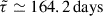 .
.
The value of  may not necessarily correspond to a PSD peak.
All Tables
All Figures
|
Fig. 1. Left panel: Thin slice of the simulated light cone. The coloured points correspond to MBHBs with Pobs ≤ 5 yr, while the black points represent all other galaxies hosted in the lightcone. We note that the lightcone slice shows some spatial periodicity of structures, which results from the box replication needed to build a wide and deep lightcone with the MSII merger trees. Right panels: Light curves in the LSST bands (u, g, r, i, z, y) associated with a MBHB at redshift ∼1.22 with mass ∼7.3 × 10⁷ M⊙, mass ratio ∼0.77 and eccentricity ∼0.24. The error bars correspond to the associated photometric uncertainty. The modelling and construction of the MBHB emission is illustrated in detail in Sections 3–4. |
| In the text | |
|
Fig. 2. Left panel: Spectral energy distribution (SED) of two selected MBHBs from our lightcone. The dashed, dotted and dash-dotted lines correspond to |
| In the text | |
|
Fig. 3. Distribution of MBHBs per deg2 as a function of magnitude. The vertical dotted and dashed lines correspond to the limiting magnitude of single and 10 yr co-added exposure modes, respectively. The dashed lines illustrate the cumulative probability functions of the full Pobs ≤ 5 yr MBHB population. In each panel, we show the number of MBHBs that are detectable in a single LSST exposure (Ndet, k, k ∈ { u, g, r, i, z, y }). |
| In the text | |
|
Fig. 4. Distribution of the MBHB properties. From left to right: Observed orbital period (Pobs), redshift (zBHB), total mass (MBHB), eccentricity (eBHB), and mass ratio (qBHB). The grey distributions correspond to the full Pobs ≤ 5 yr MBHB population inside the lightcone. The red distributions correspond to the Pobs ≤ 5 yr MBHBs detectable in the g-LSST band. The solid lines represent the corresponding cumulative distributions. |
| In the text | |
|
Fig. 5. Visualisation of the g-band variability prescribed by our templates, Δmg𝒯(z = 1), as a function of the last 30 orbits. Each panel represents a different hydrodynamical simulation from Cocchiararo et al. (2024). The template parameters (e𝒯, q𝒯) are shown in each panel. |
| In the text | |
|
Fig. 6. Example of light curve construction in the LSST g-band. The selected source features MBHB ≃ 4.91 × 10⁷ M⊙, zBHB ≃ 1.95, Pobs ≃ 2.45 yr, eBHB = 0.6, and qBHB ≃ 0.7. First panel: Random DRW realisation associated with the MBHB. Second panel: Realisation of a single mg(t) light curve. The dots represent the tailored 𝒯3 data points. The solid line implements the DRW shift from the first panel, plus the manipulations presented in Sections 4.1–4.4. Third panel: Periodogram analysis of mg(t). The vertical green dashed lines represent the Keplerian frequency and the second and third harmonics, while the corresponding shaded regions represent the frequency bin width. Finally, the vertical thick shaded grey lines mark the periodogram fmin and fmax values. |
| In the text | |
|
Fig. 7. Success rate of detecting MBHBs via variability studies in the g-band of LSST. The results are presented as a function of the MBHB properties, grouped according to the associated template. We used a total NR = 105 light curves for each MBHB, which in turn yielded a single 𝒮ℛ value per object. Each distribution thus contains Ndet, g entries. The coloured regions represent the total distribution while the horizontal segments locate the 25th, 50th, and 75th quantiles of each distribution. |
| In the text | |
|
Fig. 8. False alarm probability (FAP) in variability studies in g-LSST. The results are presented as a function of the MBHB properties, grouped according to the used template. We used a total NR = 105 light curves for each MBHB, and each distribution encloses a total of Ndet, g × 105 entries. The coloured regions represent the total distribution while the horizontal segments locate the 25th, 50th, and 75th quantiles of each distribution. In all the distributions, the peak at FAP = 10−12 corresponds to cases where we find FAP values equal to 0. |
| In the text | |
Current usage metrics show cumulative count of Article Views (full-text article views including HTML views, PDF and ePub downloads, according to the available data) and Abstracts Views on Vision4Press platform.
Data correspond to usage on the plateform after 2015. The current usage metrics is available 48-96 hours after online publication and is updated daily on week days.
Initial download of the metrics may take a while.