| Issue |
A&A
Volume 707, March 2026
|
|
|---|---|---|
| Article Number | A69 | |
| Number of page(s) | 11 | |
| Section | Catalogs and data | |
| DOI | https://doi.org/10.1051/0004-6361/202557049 | |
| Published online | 03 March 2026 | |
The first data release of J-VAR: Multi-filter light curves for 1.3 million point-like sources
1
Centro de Estudios de Física del Cosmos de Aragón, (CEFCA),
Plaza San Juan 1,
44001
Teruel
Spain
2
Centro de Astrobiología (CAB), CSIC-INTA,
Camino Bajo del Castillo s/n,
28692,
Villanueva de la Cañada,
Madrid
Spain
3
Instituto de Astrofísica de Canarias (IAC),
C/Vía Láctea s/n,
38205
La Laguna,
Tenerife
Spain
4
Departamento de Astrofísica, Universidad de La Laguna,
38205
La Laguna,
Tenerife
Spain
5
Observatório Nacional - MCTI (ON),
Rua Gal. José Cristino 77,
São Cristóvão,
20921-400
Rio de Janeiro
Brazil
6
University of Michigan, Department of Astronomy,
1085 South University Ave.,
Ann Arbor,
MI
48109
USA
7
Instituto de Astronomia, Geofísica e Ciências Atmosféricas, Universidade de São Paulo,
05508-090
São Paulo
Brazil
8
Donostia International Physics Centre (DIPC),
Paseo Manuel de Lardizabal 4,
20018
Donostia-San Sebastián
Spain
9
IKERBASQUE, Basque Foundation for Science,
48013
Bilbao
Spain
★ Corresponding author: This email address is being protected from spambots. You need JavaScript enabled to view it.
Received:
30
August
2025
Accepted:
5
January
2026
Abstract
Context. The Javalambre VARiability survey (J-VAR) is a multi-filter photometric survey conducted at the Observatorio Astrofísico de Javalambre, covering selected regions of the northern sky, and providing time-domain information for the Javalambre Photometric Local Universe Survey (J-PLUS) fields. J-VAR primarily focuses on small bodies of the Solar System, variable stars, and optical transients.
Aims. We aim to present and describe the data set of light curves contained in this first data release of J-VAR.
Methods. J-VAR observations were conducted in seven filters observed quasi-simultaneously, three SDSS broad-bands (g, r, and i), and four narrow bands of the J-PLUS filter system (J0395, J0515, J0660, and J0861). As J-VAR is executed primarily in multi-epoch mode, with multiple visits to a given field spread over a period of a year, the data were collected under varying atmospheric and sky brightness conditions. We accounted for these variations by employing an ensemble differential-photometry technique to correct the light curves, which were subsequently calibrated using already available J-PLUS photometry. Additionally, we used a classification scheme based on Bayesian neural networks to select a high-confidence sample of point-like sources (stars and quasi-stellar objects (QSOs)).
Results. J-VAR DR1 consists of 101 fields, covering about 200 square degrees on the sky and containing the light curves of more than 1.3 million point-like sources in the seven filters. The light curves span an effective magnitude range from 13 to 19, with a photometric root mean square (RMS) precision of 2% down to a magnitude of ∼16 and 5% to a magnitude of ∼18 in the broad-band filters. Furthermore, we calculated and provide a number of different variability indices for the light curves included in this data release.
Key words: techniques: photometric / catalogs / surveys / stars: variables: general
© The Authors 2026
 Open Access article, published by EDP Sciences, under the terms of the Creative Commons Attribution License (https://creativecommons.org/licenses/by/4.0), which permits unrestricted use, distribution, and reproduction in any medium, provided the original work is properly cited.
This article is published in open access under the Subscribe to Open model. This email address is being protected from spambots. You need JavaScript enabled to view it. to support open access publication.
1 Introduction
The Javalambre VARiability survey (J-VAR) is a time-domain, multi-filter, all-sky survey conducted at the Observatorio Astrofísico de Javalambre (OAJ, Cenarro et al. 2014), owned, managed, and operated by the Centro de Estudios de Física del Cosmos de Aragón (CEFCA). J-VAR was originally conceived to be observed when weather conditions (e.g. transparency, seeing, and sky background) were not suitable for one of the main OAJ surveys, the Javalambre Photometric Local Universe Survey (J-PLUS, Cenarro et al. 2019), and was designed to provide a unique combination of broad- and narrow-band filter photometry with time-domain information.
An extensive presentation of the J-VAR survey and its scientific objectives is given in an accompanying paper (Ederoclite et al., in prep.) In brief, J-VAR, through its observing strategy and the set of photometric filters employed, is designed to address three main science cases: (i) the detection and taxonomy of small Solar-System bodies (e.g. Morate et al. 2026); (ii) the detection and study of variable stars, optimised towards pulsating stars and contact binaries (e.g. a study of RR-Lyr type variables will be presented in a forthcoming paper, Kulkarni et al. 2025); and (iii) the detection and characterisation of optical transients.
Here, we describe the construction of the light-curve data set in the first J-VAR data release. The paper is organised as follows: we provide a summary of J-VAR’s survey strategy, filter setup, and observations in Sect. 2; in Sect. 3, we describe the object selection and light-curve extraction process, along with details on the photometric quality flags employed; Sect. 4 presents the ensemble differential-photometry method used to correct and calibrate the DR1 light curves; and our results, including statistics on the entire sample of light curves, pertinent information on saturation, detection, and precision limits, as well as the calculation of variability indices, are presented in Sect. 5. We end the paper with some concluding remarks and comments about data availability and access.
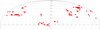 |
Fig. 1 Sky coverage of the 101 fields of J-VAR DR1 shown in equatorial coordinates. |
2 Observations, data reduction and survey strategy
The observations for J-VAR were carried out with the Javalambre Auxiliary Survey Telescope (JAST80) located at the OAJ. The JAST is an 83 cm, f/4.5 modified Ritchey-Chrétien reflector on an equatorial mount. The telescope is equipped with the T80Cam, a 9.2k × 9.2k Teledyne-e2v charge-coupled device (CCD) detector with 10 μm pixels, resulting in a 1.4 deg × 1.4 deg field of view (FoV), with a pixel scale of 0.55 arcsec pix−1 (Marin-Franch et al. 2015).
The image reduction was performed with a custom-made pipeline, called jype, developed at CEFCA for the OAJ surveys (see e.g. Cenarro et al. 2019). It is mainly implemented in python and makes use of SExtractor (Bertin & Arnouts 1996) for the source extraction and initial photometry. It has been under continuous development since 2010, and the latest version was employed for the processing of the J-VAR data.
Besides the usual image-reduction steps (bias, flat-field and fringing - when needed - corrections, masking of cosmic rays, satellite traces, etc.), it also includes the so-called illumination correction required for large FoV systems such as the JAST80. In short, when the classical flat-field correction is applied to images from telescopes with large FoV and field correctors, that typically introduces a two-dimensional bias in the photometry across the images as large as a few tens of millimagnitudes. An extra step is required to account and correct for that effect (see e.g. Appendix B.1 of Bonoli et al. 2021).
The pipeline also includes the computation of aperture corrections for photometry performed within a 6 arcsec-diameter integration area, which serves as a measure of the total flux for point-like sources and has been adopted as the reference photometry for J-VAR. J-VAR follows the exact same definitions of fields, and the associated telescope pointings, as the J-PLUS survey. J-VAR observations begin only after a given field has been observed in J-PLUS. This first data release contains a total of 101 fields, covering about 200 square degrees. The on-sky distribution of these fields is shown in Fig. 1, while a full list of the fields and their centres is given in Appendix A.
For its observations, J-VAR employs seven of the 12 filters of the J-PLUS photometric system (Cenarro et al. 2019): three of the Sloan Digital Sky Survey (SDSS, York et al. 2000) broad bands (g, r and i; Fukugita et al. 1996) and four of the narrowband filters (J0395, J0515, J0660, and J0861; Marín-Franch et al. 2012). A summary of the characteristics of the seven filters, along with information related to the observations, is given in Table 1. J-VAR observations are conducted in two modes: (i) multi-epoch observations (MEOs) and (ii) high-frequency observations (HFOs). These are described below.
MEO: In this mode, each field is visited a minimum of 11 times. The cadence between visits is not fixed, and care is taken to spread the visits over the period of about a year. In each visit (= one epoch), three images are obtained per filter. However, these same-filter observations are not consecutive; instead, the telescope cycles through the seven filters (in the order of bluer to redder wavelength) three times. This introduces a time interval of about 13 minutes between same-filter observations, as indicated in the last column of Table 1.
HFO: in the high-frequency mode, each field is visited an additional time, independently of the epoch visits. The telescope remains on the field for ∼3 hours consecutively, cycling through the seven filters, exactly as the MEO mode, until 15 images per filter are obtained. We should note, however, that weather or scheduling restrictions can occasionally interrupt the HFO mode, which is then completed on a subsequent visit to the affected field.
In this first data release, 86 of the 101 fields come with full MEO and HFO observations. The fields that include the high-frequency mode are clearly identified in the detailed list provided in Appendix A.
Seven filters of the J-PLUS photometric system used in J-VAR observations.
3 Light-curve extraction
The jype pipeline provides aperture photometry for every detected object on a given image. However, in the context of this first J-VAR data release, we aimed to provide complementary time-domain information for point-like sources included in Data Release 3 of the J-PLUS survey, and, thus, we focused on extracting the light curves for those objects. In what follows, we make extensive use of J-PLUS observations and data. Values were obtained from the relevant J-PLUS Data Release 3 (DR3) tables1, and the photometric calibration of DR3 is described in López-Sanjuan et al. (2024).
3.1 Object selection
For each field of J-VAR DR1, our starting point was the corresponding J-PLUS field-detection’s catalogue from the jplus.MagABDualObj table. This catalogue was obtained by running SExtractor on dual mode, using the SDSS r band as the reference band.
3.2 Object classification
To facilitate the selection of point sources, we subsequently used the BANNJOS algorithm (del Pino et al. 2024) to classify our objects. In short, BANNJOS uses Bayesian neural networks to classify objects in three distinct classes: STAR, QUASISTELLAR OBJECT (QSO), and GALAXY, and provides the full probability distribution function (PDF) for each class. For the purposes of J-VAR DR1, we are only interested in point-like sources, so we designed a selection based on the second and 98th percentiles (henceforth denoted pc02 and pc98) of the PDFs of each BANNJOS class, to categorise our objects in three classes, according to following criteria:
STAR: Requires class_star_pc02 > 0.33, while both class_qso_pc98 < 0.33 and class_galaxy_pc98 < 0.33.
QSO: Requires class_qso_pc02 > 0.33, while both class_star_pc98 < 0.33 and class_galaxy_pc98 < 0.33.
APS: This third category of ambiguous point sources meets the non-galaxy requirement of class_galaxy_pc98 < 0.33, but it does not strictly meet one of the other criteria that would enable it to be classified as either STAR or QSO. For example, an APS could have both class_star_pc02 > 0.33 and class_qso_pc98 >0.33.
Any object that could not be classified in one of our three categories defined above was discarded. Furthermore, within a field, and on an individual filter basis, we additionally discarded those objects that did not have valid J-PLUS photometry in the given filter.
Finally, we cross-matched our objects with the International Variable Star Index database (VSX2), as well as the variable star database (Eyer et al. 2023; Rimoldini et al. 2023) within Gaia DR3 (Gaia Collaboration 2023).
3.3 Building the light curves
With the reference-object lists, obtained from the previous step, for all field/filter combinations at hand, we proceeded to crossmatch these lists with the detection catalogues from all individual J-VAR images pertaining to the given field/filter pair. The cross-match radius was set at 1.1 arcsec, corresponding to two pixels at the pixel scale of T80Cam. Whenever a match was found, we recorded the output SExtractor flux, using a 6-arcsec aperture corrected to total flux for aperture effects.
3.4 Photometric quality flags
Apart from the native SExtractor photometric quality numerical flags, which we kept and continue to use, we implemented a few additional ones to better characterise the quality of the data points. These are added, continuing the sequence of powers of two, to the native flag values and are listed below.
Flag value 256: a stricter and more conservative saturation limit, added if the maximum pixel value within the photometric aperture exceeds 50 000 analog-to-digital units (ADU) (the original threshold in the SExtractor parameters is 60000 ADU).
Flag value 512: the object’s full width at half maximum (FWHM) on the J-VAR image exceeds the proximity limit (see below for details).
Flag value 1024: the object is cross-matched on the J-VAR catalogue, but it has invalid photometry (i.e. it is detected, but no useful measurement can be extracted).
Flag value 2048: no cross-match between the reference object list and the J-VAR detection catalogue within 1.1 arcsec.
J-VAR observations can occasionally be conducted under very poor seeing conditions, with the resulting over-broadened PSF-profiles leading to flux contamination within the photometric aperture from nearby objects. As a protective measure, we introduced the concept of proximity limit: we used the reference J-PLUS object catalogue and calculated dmin, the distance between the target object and its closest neighbour (note: this calculation is done on the original, full catalogue before we proceed to only select point sources). We then compare two numbers: (i) dmin/2 and (ii) dmin – FWHMCN, where FWHMCN is the full width at half maximum of the closest neighbour. The smallest of the two numbers is set as the proximity limit for the given target object. At the moment of light curve extraction, if the FWHM of the target object in a J-VAR image exceeds the assigned proximity limit, the corresponding data point is assigned the 512 flag value described above.
Finally, as an additional quality-control measure, we introduced the morphology flag. This is a binary flag, with the value of 1 indicating a warning. This was done to account for those cases not covered by the proximity limit, for example because the actual closest neighbour was not originally detected by SExtractor and does not appear as an entry on the reference list of objects. As the name suggests, this flag is based on the morphology of the source in the J-PLUS images. A warning value of 1 is obtained if the object’s FWHM exceeds the value of 3 arcsec or if the probability of it being a star, sglc_prob_star, from the table jplus.StarGalClass is <0.3 (see López-Sanjuan et al. 2019 for details).
3.5 Data-points-limited selection
The final set of light curves for a given field/filter pair is obtained after applying some selection criteria based on the number of valid points in a light curve. In this context, a data point is considered valid if its photometric quality flag is <1024. The criteria work hierarchically and are applied to each filter separately. They are the following: (1a) if the field has HFOs, then an object with more than nine valid data points is automatically included in the final set; (1b) those objects that do not meet the previous requirement can still be included in the final set if they have at least one valid data point in a minimum of five epochs of MEO; (2) if a field only has MEOs, then the same criterion as (1b) is applied for an object to be included in the final set.
4 Light-curve correction and calibration
Given that J-VAR observations are predominantly obtained in the MEO mode, they are affected by varying atmospheric conditions. It is therefore necessary to correct and calibrate the extracted light curves. This was achieved by employing ensemble differential photometry, a well-established technique used to improve the accuracy of photometric observations by minimising systematic errors (see e.g. Everett & Howell 2001; Tamuz et al. 2005).
In our implementation, we take full advantage of the fact that calibrated photometry for the J-VAR fields is readily available through the corresponding J-PLUS observations. We note here that, by survey design, the J-PLUS photometry is deeper than the J-VAR one. Our method is outlined in the next section.
4.1 Comparison-star selection
For each field and in each filter we first selected the available comparison stars based on their J-PLUS observations. In order for a star to be eligible, it needs to meet the criteria listed below:
The SExtractor photometric flag, obtained from the jplus.MagABDualObj table, needs to be zero (guaranteeing that the photometry is not affected by nearby objects and/or the border of the CCD, and that the object is not saturated).
Similarly, the flag related to the pixel mask, MASK_FLAG, obtained from the jplus.MagABDualObj table, needs to be zero (i.e. the background is not affected by a neighbouring very bright star).
The signal-to-noise ratio, obtained by inverting the value of the entry FLUX_RELERR_APER_3_® from the jplus.FNuDualObj table, needs to be S /N > 20 for the broad-band filters, and S/N > 15 for the narrow bands.
The morphology flag, as defined in Sect. 3, needs to be zero. • The star must not be a known variable.
These selection criteria typically left us with ∼40% of all field stars as eligible comparisons in the broad-band filters, and ∼45% for the narrow bands, with the exact numbers depending on the filter and the field source density.
4.2 Building the ensemble
For each target object, we selected its ensemble of comparison stars from the available pool, constructed in the previous step as just described, based on proximity to the target. We use a variable search radius around the target object, starting at 1 arcmin and expanding with step increments of 0.1 arcmin, until the number of comparison stars, Ncomp, contained within the search area was at least 15. This is a balancing exercise between ensuring adequate statistics and maintaining locality, to avoid inhomogeneous transparency variations across the FoV.
The process is visualised in Fig. 2, while in Fig. 3 we show the average search radius per filter required to satisfy Ncomp > 15, obtained from a sample of 500 randomly selected objects, for each field. Even in the least sensitive case of the J0395 filter, the search radius does not, on average, exceed 10 arcminutes from any given target object.
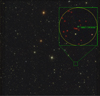 |
Fig. 2 Selection of ensemble of 17 comparison stars (red circles) within 2.9 arcmin of the target star (green circle), ensuring both adequate statistics and locality. The background image is an RGB-composite of the corresponding field obtained from J-PLUS observations and is used for illustration purposes only. |
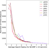 |
Fig. 3 Average search radius required to achieve Ncomp > 15, plotted against the number of objects in each field and filter. In the majority of cases, the search radius is well below 5 arcmin, with the exception of the bluest filter (J0395), which on average requires slightly larger search areas. |
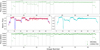 |
Fig. 4 Visualisation of our light-curve correction and calibration procedure. For clarity, all light curves are plotted as consecutive points and not according to their actual time stamps. Top panel: extracted raw light curve of a target object (green open circles) in the gSDSS filter. The star used in this example is JVAR 113038.70+241022.56 (J-PLUS ID: 84850-294) from the field 00366. The vertical dotted grey lines indicate the different epochs of observation; the two wider blocks correspond to HFO. The horizontal solid green line corresponds to the reference J-PLUS flux for this object. Middle left panel: ensemble of comparison stars selected for this target (red points). Their light curves have been normalised by their respective J-PLUS reference fluxes. The solid blue line is the master correction curve obtained. Middle right panel: family of the 500 correction curves obtained from a bootstrap process, used to assign errors on the master correction curve. Bottom panel: raw light curve (open circles) and final light curve (filled circles) obtained after applying the master correction curve. |
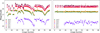 |
Fig. 5 Example light curves in all seven filters for the known eclipsing binary LINEAR 11957623 (J-PLUS ID: 94202-6998, left panel) and the non-variable star JVAR142535.72+524108.68 (J-PLUS ID: 94202-13483, right panel), selected from the same J-VAR DR1 field (02357). Both light curves are plotted as consecutive points and not according to their time stamps for clarity. |
4.3 Creating the correction curve
Once the comparison stars for a given target object have been established, their light curves are normalised by their respective J-PLUS reference flux value, fref, which is the expected calibrated total flux given the J-VAR exposure time. This is calculated via
 (1)
(1)
where  is the J-VAR exposure time in the given filter, as indicated in Table 1; magAB,f is the J-PLUS ABmagnitude from a 3 arcsec aperture in the given filter, as obtained from the jplus.MagABDualObj table; apcorr is the correction factor for aperture effects from the 3 arcsec aperture to the total, in the given filter, as obtained from the jplus.MagABDualPointSources table; and magZP is the zeropoint magnitude of the J-PLUS tile in the given filter, as obtained by the jplus.TileImage table.
Here, we adopted the 3 arcsec-corrected J-PLUS photometry as the basis for the reference total flux calculation, which is less affected by potential contamination from nearby objects. We note, however, that the 3 arcsec correction is not provided in the J-VAR photometry catalogues, so the 6 arcsec-corrected flux is used instead as the measure of the total J-VAR flux.
Finally, the normalised light curves are median-combined to obtain the master correction curve, which accounts for the changes in transparency, PSF, or other systematics present during the observations. The errors on the correction curve are calculated via a bootstrap process, the steps of which are listed below:
A comparison star from the defined ensemble for the given target is randomly selected. Its original light curve consists of N pairs of data points, the flux fn, and its associated error en ; with n = 1,..., N and N the number of individual time stamps (images).
A resampled light curve is created by drawing values from a Gaussian distribution, G (μ,σ), with μ = fn and σ = en for every data point, n. The resulting light curve is then normalised by the reference flux value of the given comparison star.
We repeat the selection of comparison stars, allowing repetition, until the number of light curves matches the number of comparison stars Ncomp. These light curves are subsequently median combined to create a resampled correction curve.
The entire process is repeated 500 times. For each time stamp, n, we assign the standard deviation of the sample of 500 correction curves to be the error of the corresponding point, n, of the master correction curve.
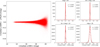 |
Fig. 6 Photometric calibration of J-VAR DR1 on J-PLUS system. Shown in this plot are the results for the rSDSS filter. Left panel: difference between the median magnitude of each J-VAR light curve and the corresponding J-PLUS magnitude. Right panels: gaussian fits to the distribution of J-VAR minus J-PLUS values for different magnitude bins, identified at the top of each panel. We also provide the mean, μ, and the standard deviation, σ, of the fitted Gaussians. |
4.4 Correcting the target light curve
In the final step, we applied the master correction curve to the raw light curve of our target object, adjusting the errors accordingly; i.e. adding, in quadrature, the photometric errors of the target light curve and the errors of the master correction curve, as derived from the bootstrap process. The corrected light curve was then converted to magnitudes on the AB scale (Oke & Gunn 1983) via
 (2)
(2)
where magJVAR is the desired J-VAR magnitude,  is the corrected J-VAR photometric flux, and
  ,
,  are the J-PLUS reference magnitude and flux, respectively.
The basic steps of the light-curve-correction process described above are visualised in Fig. 4, while in Fig. 5 we show representative examples of corrected and calibrated light curves for a variable and a non-variable object.
In order to assess the photometric calibration of this DR1, we performed the following test: for all light curves across the 101 fields in a given filter, we calculated the difference between the median light curve magnitude, < JVAR1c >, and the corresponding J-PLUS magnitude, JPLUSmag. Subsequently, we divided the light curves into four magnitude bins and proceeded to perform Gaussian fits to the distributions of < JVAR1c > - JPLUSmag values in each bin. The process was repeated for each of the seven filters. In Fig. 6, we show the results for the rSDSS filter, while in Table 2 we collect the results of all Gaussian fits, which indicate that the photometric calibration of J-VAR DR1 is entirely consistent with that of J-PLUS DR3. Finally, in Fig. 7 we show phase-folded light curves of known variable stars in DR1 as representative examples of pulsators and contact systems, towards which J-VAR is optimised.
Gaussian fits on distributions of < JVARlc > - JPLUSmag values.
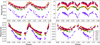 |
Fig. 7 Light curves of known variable stars in J-VAR DR1, folded on their published periods (data from VSX). A full cycle is repeated for clarity. Top left: ATO J273.8337+29.9420, a high-amplitude delta Sct (HADS); top right: LINEAR 11957623, a WUMa-type binary (EW); bottom left: LINEAR 9122839, an RRLyr-type variable (RRab); bottom right: CRTS J170902.5+25314, also an RRLyr type (RRc). |
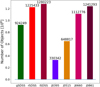 |
Fig. 8 Number of objects with light curves in J-VAR DR1 distributed across the seven filters. |
5 Results
Having described the light-curve extraction and calibration process, we now turn to exploring the resulting data set.
5.1 Statistics
J-VAR DR1 contains light curves for 1 335 279 unique pointlike sources. Of these, (i) 1 286 994 are classified as STARS (~96.4%); (ii) 15 233 are classified as QSOs (~1.1%); and (iii) 33 052 are classified as APSs (~2.5%). In Fig. 8, we show the number of objects with light curves distributed in the seven J-VAR filters. It is clear that the bluest narrow-band filters, J0395 and J0515, are considerably less sensitive than the rest.
There are over 1600 known variables from the VSX database contained within the footprint of DR1. With respect to Gaia, more than 15 200 objects are formally identified as variables (phot_variable_flag = VARIABLE in gaiadr3.gaia_source). This number is slightly reduced to ~14 700 if we further require that the variables have a class assigned to them (in_vari_classifier_result = True in gaiadr3.vari_summary); however, it is greatly reduced to just over 3100 variables if we additionally impose a confidence limit and require that the parameter best_class_score in gaiadr3.vari_classifier_result be >0.8.
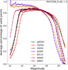 |
Fig. 9 Average percentage of valid light curve points per magnitude bin for all filters. |
5.2 Saturation and detection limits
Figure 9 shows a representation of the overall light-curve photometric quality. To construct this figure, we worked in the following fashion: for each filter, we divided all objects with light curves into magnitude bins, ranging from mag=12 to mag=21, in steps of 0.1. We took the median magnitude of a light curve to identify the corresponding bin. Within a bin and for each object, we calculated the percentage of valid photometric points with respect to the total number of points; in this context, a valid point is one with photometric flag of 0 (= no issues). Finally, we calculated the average percentage of a bin, and we plot it in Fig. 9 against magnitude. The effects of saturation and detectability are seen in the bright and faint magnitude ends, respectively. Although, note that the bluest narrow-band filters rarely saturate.
As a first approximation of quantifying the curves in Fig. 9, we arbitrarily set a limit at an average percentage value of 50 and identified, in each filter, the magnitude bins that are just below and just above the limit for the bright and faint magnitude ends. We tentatively interpret these as the saturation and detection limits and provide the corresponding magnitude values in Table 3.
5.3 Precision limits
With respect to light-curve precision, we calculated, on a perfilter basis, the limiting magnitude up to which a light curve is expected to have a certain precision value. This was done by first calculating the RMS of each light curve in a given filter. Again, we used the median value of the light curve as a representative value for the magnitude of each object. Subsequently, for a grid of RMS values ranging from 0.01 to 0.2 in steps of 0.01, we selected all objects with an RMS below the given value and set the 95th percentile of the magnitudes of objects meeting the RMS criterion as the corresponding magnitude limit. We plot the results in Fig. 10 and give a sample of representative values in Table 4.
Saturation and detection limits per filter.
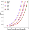 |
Fig. 10 Expected limiting magnitude for an object to have a light curve with a certain RMS value in each of the seven filters. |
Representative light-curve RMS values in all filters.
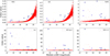 |
Fig. 11 Example of variability indices calculated from light curves of field 00056 in the rSDSS filter. Known variables within the VSX database are indicated by blue squares, while those from Gaia are shown by green diamonds. The indices were calculated under the requirement that valid points have a photometric quality flag equal to zero. |
5.4 Variability indices
As a first, practical, application of the resulting data set, we calculated a series of variability indices (see Sokolovsky et al. 2017, among others, for a comprehensive review) for each available light curve in DR1. The various indices were calculated in two ways, using different definitions for the validity of the photometric points making up the light curves. (i) First, we considered a point to be valid if its photometric flag was less than 1024; under this constraint, our data-point-limited selection described in Sect. 3.5 ensures a minimum of five data points for each light curve, allowing at least some of the indices (see below) to be calculated for every light curve. (ii) Second, we used a more restrictive calculation, where data points were considered valid only if their photometric quality flag was equal to zero, with the additional constraint that at least five such points were required for an index to be calculated. We note that, regardless of the method used for the calculation, not every index could be calculated for every light curve. Figure 11 shows a representative example of the variability indices obtained from one of the DR1 fields. The indices calculated are the following:
Median absolute deviation (MAD): The MAD, for a light curve consisting of mi data points is given by
 (3)
(3)
Interquartile range (IQR): The IQR is defined as the difference between the upper quartile, Q3, corresponding to the 75th percentile, and the lower quartile, Q1, corresponding to the 25th percentile of the data set:
 (4)
(4)
Robust median statistic (RoMS): The RoMS (Enoch et al. 2003), for a light curve consisting of a total of N data points, mi, with their associated errors, σi, is defined as
 (5)
(5)
The three indices described above were calculated for every light curve in DR1, under the requirement that the photometric flag of valid points is less than 1024. Additionally, whenever possible, we also calculated the following indices:
The von Neumann ratio: The von Neumann ratio, denoted as η (von Neumann 1941, 1942), is defined as the ratio of the meansquare successive difference to the distribution variance. In our implementation, to ensure that variable objects have large values of the index in line with the rest of the indices, we used the inverted von Neumann ratio, given by
 (6)
(6)
with
 (7)
(7)
being the variance and
 (8)
(8)
the mean-square successive difference.
We note that care needs to be taken when calculating 1∕η in the case of J-VAR light curves, considering data obtained in the MEO mode. Within a given epoch with three observations per filter, we have two successive pairs of images, (1st, 2nd) and (2nd, 3rd). However, the third image of an epoch and the first image of the next epoch cannot be considered successive observations and do not enter in the calculation of δ2. Additionally, the variance σ2, in our case, is calculated only from those points that also enter in the δ2 calculation.
Welch-Stetson index I: The Welch-Stetson variability index I (Welch & Stetson 1993) characterises the degree of correlation between (quasi-)simultaneous pairs of observations obtained in different filters. In our case, pairing the gSDSS and rSDSS observations (with an average time difference of ∆T = 144.5 s between exposures) the Welch-Stetson index is given by
 (9)
(9)
We additionally calculated the Welch-Stetson index by pairing the rSDSS and iSDSS observations, with an average time difference of ∆T = 246 s.
6 Summary
In this paper, we present the light-curve data set of J-VAR Data Release 1. We used a Bayesian neural network to select point-like sources from an input catalogue obtained from the J-PLUS survey and subsequently classified them as stars, QSOs, or ambiguous point sources. We employed an ensemble differential photometry technique to correct the extracted light curves and made use of available J-PLUS DR3 photometry to calibrate them, while carefully monitoring the photometric quality of the data points through the use of a variety of quality flags. We conducted and presented a series of statistical tests in order to provide interested users with a detailed view of the released data set. Finally, we used the obtained set of light curves to calculate a number of variability indices for the point-like sources contained in DR1. An in-depth look at the variability indices, as well as a number of new variable star detections, will be the subject of a future publication.
Data availability
All the light curves and variability indices of J-VAR Data Release 1 are publicly available from CEFCA’s Archive webpages accessible via the following link: https://archive.cefca.es/catalogues/jvar-dr1.
Acknowledgements
We thank the anonymous referee for a constructive report which helped improved this manuscript. Based on observations made with the JAST80 telescope at the Observatorio Astrofísico de Javalambre (OAJ), in Teruel, owned, managed, and operated by the Centro de Estudios de Física del Cosmos de Aragón. We acknowledge the OAJ Data Processing and Archiving Department (DPAD) for reducing the OAJ data used in this work, as well as the distribution of the data products through a dedicated web portal. We gratefully acknowledge funding from the Governments of Spain and Aragón through their general budgets and the Fondo de Inversiones de Teruel. SP, AE, HVR and DM acknowledge funding from the Spanish Ministry of Science and Innovation (MCIN/AEI/10.13039/501100011033) and ERDF: A way of making Europe, with grant PID2021-124918NB-C42. AE acknowledges the financial support from the Spanish Ministry of Science and Innovation and the European Union - NextGenerationEU through the Recovery and Resilience Facility project ICTS-MRR-2021-03-CEFCA. DM acknowledges the financial support from the European Union - NextGenerationEU through the Recovery and Resilience Facility program Planes Complementarios con las CCAA de Astrofísica y Física de Altas Energías - LA4. This research was partially funded by MICIU/AEI/10.13039/501100011033/ through grant PID2023-146210NB-100. Funding for the J-PLUS Project has been provided by the Governments of Spain and Aragón through the Fondo de Inversiones de Teruel; the Aragonese Government through the Research Groups E96, E103, E16_17R, E16_20R, and E16_23R; the Spanish Ministry of Science and Innovation (MCIN/AEI/10.13039/501100011033 y FEDER, Una manera de hacer Europa) with grants PID2021-124918NB-C41, PID2021-124918NB-C42, PID2021-124918NA-C43, and PID2021-124918NB-C44; the Spanish Ministry of Science, Innovation and Universities (MCIU/AEI/FEDER, UE) with grants PGC2018-097585-B-C21 and PGC2018-097585-B-C22; the Spanish Ministry of Economy and Competitiveness (MINECO) under AYA2015-66211-C2-1-P, AYA2015-66211-C2-2, AYA2012-30789, and ICTS-2009-14; and European FEDER funding (FCDD10-4E-867, FCDD13-4E-2685). The Brazilian agencies FINEP, FAPESP, and the National Observatory of Brazil have also contributed to this project. This research has made use of the International Variable Star Index (VSX) database, operated at AAVSO, Cambridge, Massachusetts, USA; Astropy, a community-developed core Python package for Astronomy (Astropy Collaboration 2013); and Matplotlib, a 2D graphics package used for Python for publication-quality image generation across user interfaces and operating systems (Hunter 2007).
References
- Astropy Collaboration (Robitaille, T. P., et al.) 2013, A&A, 558, A33 [NASA ADS] [CrossRef] [EDP Sciences] [Google Scholar]
- Bertin, E., & Arnouts, S. 1996, A&AS, 117, 393 [NASA ADS] [CrossRef] [EDP Sciences] [Google Scholar]
- Bonoli, S., Marín-Franch, A., Varela, J., et al. 2021, A&A, 653, A31 [NASA ADS] [CrossRef] [EDP Sciences] [Google Scholar]
- Cenarro, A. J., Moles, M., Marín-Franch, A., et al. 2014, SPIE Conf. Ser., 9149, 91491I [NASA ADS] [Google Scholar]
- Cenarro, A. J., Moles, M., Cristóbal-Hornillos, D., et al. 2019, A&A, 622, A176 [NASA ADS] [CrossRef] [EDP Sciences] [Google Scholar]
- del Pino, A., López-Sanjuan, C., Hernán-Caballero, A., et al. 2024, A&A, 691, A221 [NASA ADS] [CrossRef] [EDP Sciences] [Google Scholar]
- Enoch, M. L., Brown, M. E., & Burgasser, A. J. 2003, AJ, 126, 1006 [NASA ADS] [CrossRef] [Google Scholar]
- Everett, M. E., & Howell, S. B. 2001, PASP, 113, 1428 [Google Scholar]
- Eyer, L., Audard, M., Holl, B., et al. 2023, A&A, 674, A13 [NASA ADS] [CrossRef] [EDP Sciences] [Google Scholar]
- Fukugita, M., Ichikawa, T., Gunn, J. E., et al. 1996, AJ, 111, 1748 [Google Scholar]
- Gaia Collaboration (Vallenari, A., et al.) 2023, A&A, 674, A1 [NASA ADS] [CrossRef] [EDP Sciences] [Google Scholar]
- Hunter, J. D. 2007, Comput. Sci. Eng., 9, 90 [NASA ADS] [CrossRef] [Google Scholar]
- Kulkarni, S., Vázquez Ramió, H., López-SanJuan, C., Ederoclite, A., & Pyrzas, S. 2025, OJAp, submitted [arXiv:2509.03120] [Google Scholar]
- López-Sanjuan, C., Vázquez Ramió, H., Varela, J., et al. 2019, A&A, 622, A177 [Google Scholar]
- López-Sanjuan, C., Vázquez Ramió, H., Xiao, K., et al. 2024, A&A, 683, A29 [NASA ADS] [CrossRef] [EDP Sciences] [Google Scholar]
- Marín-Franch, A., Chueca, S., Moles, M., et al. 2012, SPIE Conf. Ser., 8450, 84503S [Google Scholar]
- Marin-Franch, A., Taylor, K., Cenarro, J., Cristobal-Hornillos, D., & Moles, M. 2015, in IAU General Assembly, 29, 2257381 [Google Scholar]
- Morate, D., Mahlke, M., Álvarez-Candal, A., et al. 2026, MNRAS, 545, 2052 [Google Scholar]
- Oke, J. B., & Gunn, J. E. 1983, ApJ, 266, 713 [NASA ADS] [CrossRef] [Google Scholar]
- Rimoldini, L., Holl, B., Gavras, P., et al. 2023, A&A, 674, A14 [NASA ADS] [CrossRef] [EDP Sciences] [Google Scholar]
- Sokolovsky, K. V., Gavras, P., Karampelas, A., et al. 2017, MNRAS, 464, 274 [CrossRef] [Google Scholar]
- Tamuz, O., Mazeh, T., & Zucker, S. 2005, MNRAS, 356, 1466 [Google Scholar]
- von Neumann, J. 1941, Ann. Math. Stat., 12, 367 [Google Scholar]
- von Neumann, J. 1942, Ann. Math. Stat., 13, 86 [Google Scholar]
- Welch, D. L., & Stetson, P. B. 1993, AJ, 105, 1813 [NASA ADS] [CrossRef] [Google Scholar]
- York, D. G., Adelman, J., Anderson, Jr., J. E., et al. 2000, AJ, 120, 1579 [NASA ADS] [CrossRef] [Google Scholar]
Available at https://archive.cefca.es/catalogues/jplus-dr3
Appendix A The fields of DR1
The 101 fields of J-VAR DR1.
All Tables
All Figures
|
Fig. 1 Sky coverage of the 101 fields of J-VAR DR1 shown in equatorial coordinates. |
| In the text | |
|
Fig. 2 Selection of ensemble of 17 comparison stars (red circles) within 2.9 arcmin of the target star (green circle), ensuring both adequate statistics and locality. The background image is an RGB-composite of the corresponding field obtained from J-PLUS observations and is used for illustration purposes only. |
| In the text | |
|
Fig. 3 Average search radius required to achieve Ncomp > 15, plotted against the number of objects in each field and filter. In the majority of cases, the search radius is well below 5 arcmin, with the exception of the bluest filter (J0395), which on average requires slightly larger search areas. |
| In the text | |
|
Fig. 4 Visualisation of our light-curve correction and calibration procedure. For clarity, all light curves are plotted as consecutive points and not according to their actual time stamps. Top panel: extracted raw light curve of a target object (green open circles) in the gSDSS filter. The star used in this example is JVAR 113038.70+241022.56 (J-PLUS ID: 84850-294) from the field 00366. The vertical dotted grey lines indicate the different epochs of observation; the two wider blocks correspond to HFO. The horizontal solid green line corresponds to the reference J-PLUS flux for this object. Middle left panel: ensemble of comparison stars selected for this target (red points). Their light curves have been normalised by their respective J-PLUS reference fluxes. The solid blue line is the master correction curve obtained. Middle right panel: family of the 500 correction curves obtained from a bootstrap process, used to assign errors on the master correction curve. Bottom panel: raw light curve (open circles) and final light curve (filled circles) obtained after applying the master correction curve. |
| In the text | |
|
Fig. 5 Example light curves in all seven filters for the known eclipsing binary LINEAR 11957623 (J-PLUS ID: 94202-6998, left panel) and the non-variable star JVAR142535.72+524108.68 (J-PLUS ID: 94202-13483, right panel), selected from the same J-VAR DR1 field (02357). Both light curves are plotted as consecutive points and not according to their time stamps for clarity. |
| In the text | |
|
Fig. 6 Photometric calibration of J-VAR DR1 on J-PLUS system. Shown in this plot are the results for the rSDSS filter. Left panel: difference between the median magnitude of each J-VAR light curve and the corresponding J-PLUS magnitude. Right panels: gaussian fits to the distribution of J-VAR minus J-PLUS values for different magnitude bins, identified at the top of each panel. We also provide the mean, μ, and the standard deviation, σ, of the fitted Gaussians. |
| In the text | |
|
Fig. 7 Light curves of known variable stars in J-VAR DR1, folded on their published periods (data from VSX). A full cycle is repeated for clarity. Top left: ATO J273.8337+29.9420, a high-amplitude delta Sct (HADS); top right: LINEAR 11957623, a WUMa-type binary (EW); bottom left: LINEAR 9122839, an RRLyr-type variable (RRab); bottom right: CRTS J170902.5+25314, also an RRLyr type (RRc). |
| In the text | |
|
Fig. 8 Number of objects with light curves in J-VAR DR1 distributed across the seven filters. |
| In the text | |
|
Fig. 9 Average percentage of valid light curve points per magnitude bin for all filters. |
| In the text | |
|
Fig. 10 Expected limiting magnitude for an object to have a light curve with a certain RMS value in each of the seven filters. |
| In the text | |
|
Fig. 11 Example of variability indices calculated from light curves of field 00056 in the rSDSS filter. Known variables within the VSX database are indicated by blue squares, while those from Gaia are shown by green diamonds. The indices were calculated under the requirement that valid points have a photometric quality flag equal to zero. |
| In the text | |
Current usage metrics show cumulative count of Article Views (full-text article views including HTML views, PDF and ePub downloads, according to the available data) and Abstracts Views on Vision4Press platform.
Data correspond to usage on the plateform after 2015. The current usage metrics is available 48-96 hours after online publication and is updated daily on week days.
Initial download of the metrics may take a while.