| Issue |
A&A
Volume 707, March 2026
|
|
|---|---|---|
| Article Number | A333 | |
| Number of page(s) | 12 | |
| Section | Galactic structure, stellar clusters and populations | |
| DOI | https://doi.org/10.1051/0004-6361/202557219 | |
| Published online | 19 March 2026 | |
photoD with Rubin’s Data Preview 1: First stellar photometric distances and faint blue star deficits
Stellar distances with Rubin’s DP1
1
Ruđer Bošković Institute,
Bijenička cesta 54,
10000
Zagreb,
Croatia
2
XV. Gymnasium (MIOC),
Jordanovac 8,
10000
Zagreb,
Croatia
3
Vera C. Rubin Observatory Project Office,
950 N. Cherry Ave.,
Tucson,
AZ
85719,
USA
4
University of Washington, Dept. of Astronomy,
Box 351580,
Seattle,
WA
98195,
USA
5
Faculty of Physics, University of Rijeka,
Radmile Matejčić 2,
Rijeka,
Croatia
6
Institute for Data-intensive Research in Astrophysics and Cosmology, University of Washington,
3910 15th Avenue NE,
Seattle,
WA
98195,
USA
7
McWilliams Center for Cosmology & Astrophysics, Department of Physics, Carnegie Mellon University,
Pittsburgh,
PA
15213,
USA
8
Olympic College,
1600 Chester Ave.,
Bremerton,
WA
98337-1699,
USA
9
INAF – Osservatorio Astronomico di Padova,
Vicolo dell‘Osservatorio 5,
35122
Padova,
Italy
10
Department of Physics and Astronomy G. Galilei, University of Padova,
Vicolo dell’Osservatorio 3,
35122
Padova,
Italy
11
SLAC National Accelerator Laboratory,
2575 Sand Hill Rd.,
Menlo Park,
CA
94025,
USA
12
Université Paris Cité, CNRS/IN2P3, CEA, APC,
4 rue Elsa Morante,
75013
Paris,
France
13
Yerkes Observatory,
373 W. Geneva St.,
Williams Bay,
WI
53191,
USA
14
Vera C. Rubin Observatory/NSF NOIRLab,
950 N. Cherry Ave.,
Tucson,
AZ
85719,
USA
15
Université Paris Cité, CNRS/IN2P3, APC,
4 rue Elsa Morante,
75013
Paris,
France
16
Kavli Institute for Particle Astrophysics and Cosmology, SLAC National Accelerator Laboratory,
2575 Sand Hill Rd.,
Menlo Park,
CA
94025,
USA
17
NSF NOIRLab,
950 N. Cherry Ave.,
Tucson,
AZ
85719,
USA
18
Université Paris-Saclay, CNRS/IN2P3, IJCLab,
15 Rue Georges Clemenceau,
91405
Orsay,
France
19
Vera C. Rubin Observatory,
Avenida Juan Cisternas #1500,
La Serena,
Chile
20
Sorbonne Université, Université Paris Cité, CNRS/IN2P3, LPNHE,
4 place Jussieu,
75005
Paris,
France
21
Santa Cruz Institute for Particle Physics and Physics Department, University of California–Santa Cruz,
1156 High St.,
Santa Cruz,
CA
95064,
USA
22
Steward Observatory, The University of Arizona,
933 N. Cherry Ave.,
Tucson,
AZ
85721,
USA
23
Université Clermont Auvergne, CNRS/IN2P3, LPCA,
4 Avenue Blaise Pascal,
63000
Clermont-Ferrand,
France
24
University of Arizona, Department of Astronomy and Steward Observatory,
933 N. Cherry Ave,
Tucson,
AZ
85721,
USA
25
Department of Astronomy, Yonsei University,
50 Yonsei-ro,
Seoul
03722,
Republic of Korea
26
Physics Department, University of California,
One Shields Avenue,
Davis,
CA
95616,
USA
27
Physics Department, University of California,
366 Physics North, MC 7300
Berkeley,
CA
94720,
USA
28
Department of Physics, Duke University,
Durham,
NC
27708,
USA
29
Department of Astrophysical Sciences, Princeton University,
Princeton,
NJ
08544,
USA
30
Brookhaven National Laboratory,
Upton,
NY
11973,
USA
31
CNRS/IN2P3, CC-IN2P3,
21 avenue Pierre de Coubertin,
69627
Villeurbanne,
France
32
NCSA, University of Illinois at Urbana-Champaign,
1205 W. Clark St.,
Urbana,
IL
61801,
USA
33
Department of Physics and Astronomy, Purdue University,
525 Northwestern Ave.,
West Lafayette,
IN
47907,
USA
34
National Institute of Standards and Technology, Material Measurement Laboratory, Office of Data and Informatics,
Gaithersburg,
MD,
USA
35
Florida Institute of Technology,
150 W. University Blvd.,
Melbourne,
FL
32901,
USA
36
Lawrence Livermore National Laboratory,
7000 East Avenue,
Livermore,
CA
94550,
USA
37
Space Telescope Science Institute,
3700 San Martin Drive,
Baltimore,
MD
21218,
USA
38
Austin Peay State University,
Clarksville,
TN
37044,
USA
39
ASTRON,
Oude Hoogeveensedijk 4,
7991
PD,
Dwingeloo,
The Netherlands
40
Fermi National Accelerator Laboratory,
PO Box 500,
Batavia,
IL
60510,
USA
41
Department of Physics, Harvard University,
17 Oxford St.,
Cambridge,
MA
02138,
USA
42
LSST Discovery Alliance,
933 N. Cherry Ave.,
Tucson,
AZ
85719,
USA
★ Corresponding author: This email address is being protected from spambots. You need JavaScript enabled to view it.
Received:
12
September
2025
Accepted:
28
January
2026
Abstract
Aims. We investigate the utility of Rubin’s Data Preview 1 (DP1) for estimating stellar number density profiles across the Milky Way halo.
Methods. We used stellar broad-band near-UV to near-IR ugrizy photometry released in Rubin’s DP1 to estimate distance and metallicity for blue main sequence stars brighter than r = 24 in three ~1.1 sq. deg. fields at southern Galactic latitudes.
Results. Compared to TRILEGAL simulations of the Galaxy’s stellar content, we found a likely deficit of blue main sequence turn-off stars with 22 < r < 24. We interpreted this discrepancy as a signature of a steeper halo number density profile at galactocentric distances 10–50 kpc than the canonical ~1/r3 profile assumed in TRILEGAL simulations.
Conclusions. This interpretation is consistent with earlier suggestions based on observations of more luminous, but much less numerous, evolved stellar populations, along with a few pencil beam surveys of blue main sequence stars in the northern sky. These results bode well for the future Galactic halo exploration with Rubin’s Legacy Survey of Space and Time (LSST).
Key words: stars: distances / Galaxy: fundamental parameters / Galaxy: general / Galaxy: halo / Galaxy: stellar content / Galaxy: structure
© The Authors 2026
 Open Access article, published by EDP Sciences, under the terms of the Creative Commons Attribution License (https://creativecommons.org/licenses/by/4.0), which permits unrestricted use, distribution, and reproduction in any medium, provided the original work is properly cited.
This article is published in open access under the Subscribe to Open model. This email address is being protected from spambots. You need JavaScript enabled to view it. to support open access publication.
1 Introduction
Thanks to the advent of sensitive wide-area digital sky surveys, the last two decades have seen tremendous progress in mapping of the Galaxy’s principal components: the bulge, the thin and thick disks, and the halo (e.g., Bahcall 1986; Ivezić et al. 2012; Stringer et al. 2021; Feng et al. 2024; Yu et al. 2024; Medina et al. 2024; Fukushima et al. 2025). Studies of the Galactic stellar halo provide especially powerful clues for the Galaxy’s formation and evolution history due to its long dynamical time scales. This region also provides unique constraints for the Galaxy’s total mass and extent, which are important parameters for near-field cosmology.
The distant stellar halo profile was first measured beyond a galactocentric distance of rgc ~ 10 kpc by Wetterer & McGraw (1996). They analyzed the distribution of RR Lyrae stars and estimated that the stellar number density profile (hereafter, the radial profile) follows a ![Mathematical equation: $\[1 / r_{g c}^{n}\]$](/articles/aa/full_html/2026/03/aa57219-25/aa57219-25-eq1.png) power law with n ~3 out to ~80 kpc. More recent studies of RR Lyrae stars and other luminous tracers, such as blue horizontal branch stars and M giants, found evidence that the radial profile steepens beyond about 30 kpc (e.g., Faccioli et al. 2014; Han et al. 2022; Yu et al. 2024; Fukushima et al. 2025). For example, Fig. 7 in Medina et al. (2024) visually summarizes the radial profile versus rgc results from many studies and shows that at about rgc ~ 20–30 kpc, the profile power-law index n changes from about 2–3 to about 4–5. Similar conclusions were drawn using main sequence stars (typically blue turn-off stars) observed in a few small-area pencil beam surveys (e.g., Sesar et al. 2011) and from a global fitting of colour-magnitude diagrams down to g=23 from the Dark Energy Survey (DES), covering 2300 deg2 (Pieres et al. 2020). These findings are important for understanding the accretion history of the Milky Way. For example, based on a comparison to numerical simulations, Deason et al. (2014) found that stellar halos with shallower slopes at large distances tend to have more recent accretion activity and concluded that steeper observed slopes suggest that the Milky Way has had a relatively quiet accretion history over the past several billion years.
power law with n ~3 out to ~80 kpc. More recent studies of RR Lyrae stars and other luminous tracers, such as blue horizontal branch stars and M giants, found evidence that the radial profile steepens beyond about 30 kpc (e.g., Faccioli et al. 2014; Han et al. 2022; Yu et al. 2024; Fukushima et al. 2025). For example, Fig. 7 in Medina et al. (2024) visually summarizes the radial profile versus rgc results from many studies and shows that at about rgc ~ 20–30 kpc, the profile power-law index n changes from about 2–3 to about 4–5. Similar conclusions were drawn using main sequence stars (typically blue turn-off stars) observed in a few small-area pencil beam surveys (e.g., Sesar et al. 2011) and from a global fitting of colour-magnitude diagrams down to g=23 from the Dark Energy Survey (DES), covering 2300 deg2 (Pieres et al. 2020). These findings are important for understanding the accretion history of the Milky Way. For example, based on a comparison to numerical simulations, Deason et al. (2014) found that stellar halos with shallower slopes at large distances tend to have more recent accretion activity and concluded that steeper observed slopes suggest that the Milky Way has had a relatively quiet accretion history over the past several billion years.
However, Medina et al. (2024) emphasized that results for the radial profile seem to depend on the regions of the sky surveyed, implying that for robust conclusions large sky areas must be examined. Furthermore, the spatial resolution for mapping the halo can be greatly enhanced by studying main sequence stars, which are much more numerous than the more luminous stellar populations. In order to explore the halo to distances of ~100kpc (distance modulus of 20 mag) with turn-off stars (absolute magnitude Mr ~ 5), a sky survey with reliable star-galaxy separation performance to r ~ 25 is needed. With ground-based seeing of the order 1 arcsec, the 5σ limiting depth of r ~ 27 is required to ensure such performance due to galaxies vastly outnumbering stars at such faint apparent magnitudes (Slater et al. 2020). Therefore, a large-area sky survey with the 5σ limiting depth of r ~ 27 is required to explore the distant halo with numerous main sequence stars.
The upcoming Legacy Survey of Space and Time (LSST) about to be started at the NSF-DOE Vera C. Rubin Observatory (Ivezić et al. 2019) meets these requirements for sky coverage and depth. Over its main 18 000 deg2 footprint, LSST is expected to reach a depth of r~27 (Bianco et al. 2022). The Rubin Observatory recently released their Data Preview 1 (NSF-DOE Vera C. Rubin Observatory 2025, hereafter, DP1), which the first public dataset based on commissioning observations with an engineering camera (SLAC & NSF-DOE Vera C. Rubin Observatory 2024). Despite being much smaller and shallower than the ultimate LSST dataset (apart from the Extended Chandra Deep Field South, ECDFS), DP1 presents the first opportunity to assess the potential of LSST, to test its data quality and processing pipeline performance, and check various tools that are being developed to distribute and analyze LSST data.
One such tool is a Bayesian software framework for rapid estimation of distance, metallicity, and interstellar dust extinction along the line of sight for stars in the Galaxy (Palaversa et al. 2025). This framework, named photoD, will be applied to future LSST data releases and here we provide the first test of its performance on real Rubin data. We briefly overview our methodology and describe the DP1 dataset in Sect. 2. We present our analysis in Sect. 3 and summarize and discuss our results and possibilities for further improvements in Sect. 4.
2 Methodology
In this section, we describe the data used in our analysis, selection of the final stellar samples, and the method used for estimating stellar distances and photometric metallicity.
2.1 Rubin Observatory’s DP1 photometry
Several papers have already utilized DP1 for galactic studies (Choi et al. 2025; Wainer et al. 2025; Carlin et al. 2025; Malanchev et al. 2025). We used the Rubin Science Platform’s Table Access Protocol to obtain b_free_psfFlux1. fluxes from the Object catalog for each of the seven DP1 fields. Each of these fields covers an area of approximately 1.1 deg2. and their locations are illustrated in Fig. 1 (adapted from (NSF-DOE Vera C. Rubin Observatory 2025)2). The released data contain observations taken from October 24 to December 11, 2024 and include a total of about 2000 30- or 38-second exposures taken through Rubin ugrizy filters by the engineering camera (LSSTComCam)3. The LSSTComCam contains a single “raft” of nine 4k × 4k CCDs arranged in a 3 × 3 square grid and placed in the center of the Simonyi Survey Telescope’s field of view. The plate scale of the images is equal to that of the full LSSTCam; however, the total field of view is significantly smaller (by 21 times).
Because of the commissioning requirements, the cadence of the observations was significantly different for each of the fields. Additionally the 47 Tuc, Rubin SV 38 7, Fornax dwarf spheroidal galaxy, and Seagull nebula fields had less than ten visits in either u or i filters. Therefore, we excluded those fields from our analyses and focused our investigations on the three best-observed fields: ECDFS, Euclid Deep Field South (EDFS), and Rubin SV 95 −25. Further details about these fields, such as sky locations and the number of exposures per band, are listed in Tables 1 and 2. The integrated depth of an unresolved source at the S/N of 5 (5σ) is in the 26.0 ≲ r ≲ 26.8 range for the three fields studied in this paper (approximately, the ECDFS depth is comparable to a ten-year LSST survey while the other two fields correspond to about three to four years of LSST data). The selection of stellar candidates from these catalogs is discussed below.
2.2 Additional photometry from extant catalogs
To validate the results obtained from the Rubin DP1, we utilized photometric catalogs derived from observations made by the Dark Energy Camera (DECam) on the 4-meter Blanco Telescope. Corresponding catalogs were published as part of the DES Data Release 2 (DR2, Abbott et al. 2021) and the DECam Local Volume Exploration (DELVE Drlica-Wagner et al. 2022) survey DR2. These surveys provide the deepest optical observations of the three DP1 fields investigated in this paper.
The DES DR2 catalog is derived from coadded images assembled from six years of observations and covers about 5000 deg2 in the grizY bands. Its sky coverage includes Rubin DP1 ECDFS and EDFS fields. In the filters relevant to this work, the median coadded catalog depth in a 1.95 arcsec aperture at signal-to-noise ratios of S/N=5 is g=25.4, r=25.1, and i=24.5. The photometric accuracy is estimated at approximately 11 mmag and the photometric uniformity has a standard deviation of less than 3 mmag. To select high-confidence photometry and separate extended and point-like sources we require for each gri band (b) that flags_b < 4, imaflags_iso_b == 0 and extended_class_coadd < = 0.
The DELVE Data Release 2 combines public archival DECam data with more than 150 nights of additional observations for a total coverage of more than 21 000 deg2 of the high-Galactic-latitude sky that includes the Rubin SV 95 −25 field. The median PSF depth for point like sources in the g, r, i bands at S/N=5 is estimated at 24.2, 23.8, and 23.4 mag, respectively, while the absolute photometric uncertainty is ⪅ 20 mmag. To separate extended and point-like sources, we require that the gri bands simultaneously satisfy the condition EXTENDED_CLASS_b == 0, where b stands for band.
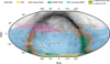 |
Fig. 1 Sky coverage of Rubin DP1 dataset. The seven LSSTComCam fields are shown as yellow dots (with names) in the context of the LSST’s planned regions: North Ecliptic Spur (purple), South Celestial Pole (yellow), the dusty plane, the Galactic Plane and Magellanic Clouds (brown and green), and low-dust-extinction regions of the Wide-Fast-Deep (blue) program. Here, we analyze data from three fields: ECDFS, EDFS, and Rubin SV 95 −25. |
Characteristics of the three Rubin DP1 fields and the selection process.
Median 5σ coadded point-source detection limits per field and band.
2.3 Star-galaxy separation with DP1 photometry
Selection of unresolved sources, popularly known as star-galaxy separation4, is an important methodological step because its limitations can result in both incomplete and contaminated samples of unresolved objects, presumably stars. These difficulties are exacerbated at the faint magnitudes probed by Rubin because galaxies can outnumber stars by more than an order of magnitude at high galactic latitudes.
The Rubin DP1 Object and Source catalogs include extendedness, a binary quantity provided in each bandpass. It is set to unity when the point spread function (PSF) magnitude exceeds the CModel magnitude5 by 0.016 mag, indicating statistical evidence of a resolved source. The statistical properties of this “star-galaxy separator,” and its comparison to analogous quantities, such as EXTENDED_CLASS used by the DES pipelines, are discussed in detail by Slater et al. (2020).
Given that extendedness values in each bandpass are measured nearly independently, they can be combined to increase the accuracy of star-galaxy separation. The optimal probabilistic approach is described in Slater et al. (2020) and relies on a quantitative description of the source distribution in the CModel versus PSF magnitude space, as well as on adequate Bayesian priors. Since neither one is available for the DP1 dataset at present, we employed an ansatz to combine measurements from the gri bandpasses, as follows.
Figure 2 shows the variation of the difference of the CModel and PSF magnitudes as a function of magnitude. The distribution of sources in this diagram is similar in the three shown bands with the highest S/N and we took the mean of the three values. This averaging operation results in a somewhat narrower distribution between the difference of CModel and PSF magnitudes for the vertical plume corresponding to unresolved sources, although it is not possible to precisely quantify the improvement in star-galaxy separation without adequate training samples. Using the mean value, we selected candidates for unresolved sources by limiting the magnitude difference to 0.04 mag (see the bottom right panel in Fig. 3). The adopted value is larger than the default value of 0.016 mag adopted by Rubin pipelines and is motivated by the morphology of the source distribution. We selected a criterion more inclusive than the default because we will discuss below a deficit of faint blue stars. In other words, we chose to err on the side of galaxy contamination in the stellar sample, rather than stellar sample incompleteness.
Using this method, we construct separate color–magnitude diagrams for unresolved and resolved sources shown in Fig. 4. The morphology of the source distribution in those diagrams clearly indicates that the much less numerous stellar sample becomes contaminated by galaxies for r > 24. This contamination could be alleviated somewhat statistically with appropriate use of priors (Slater et al. 2020).
Priors are usually computed using simulations of the Milky Way stellar content, such as TRILEGAL (Dal Tio et al. 2022). TRILEGAL is a state-of-the-art simulation of anticipated LSST stellar content and is publicly accessible via NOIRLab’s Astro Data Lab6. We report here a detection of a faint cutoff in the distribution of blue stars (g − r < 0.6) at r ~ 22 that is in strong conflict with predictions of the TRILEGAL model. For this reason, using TRILEGAL-based priors in the star-galaxy separation step would appear to be premature. We proceed to discuss this empirical finding of a deficit in the counts of faint blue stars in more detail below.
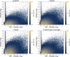 |
Fig. 2 Difference between the PSF (point spread function) magnitude and the CModel magnitude in the gri bands, and the mean gri value (bottom right) vs. magnitude for the ECDFS field (analogous to Fig. 1 from Slater et al. 2020). The colormap encodes the number of stars per bin. The bimodal distribution of stars and galaxies (more precisely, unresolved and resolved sources) is evident. |
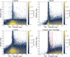 |
Fig. 3 Same as Fig. 2, except that the abscissa is zoomed in on, and the left panels show the u and y band diagrams, respectively. The two vertical lines in the bottom right panel show the separation boundary between unresolved and resolved sources (dashed at 0.016 mag: Rubin default value for single-band classification; solid at 0.04 mag: adopted here for the mean gri values and designed to ensure stellar completeness to faint magnitude limits). |
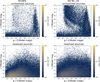 |
Fig. 4 Comparison of color–magnitude diagrams of unresolved (top) and resolved (bottom) sources selected from Rubin DP1 fields ECDFS (left) and SV 95 −25 (right). Note: low fractions of unresolved sources (approximately 8% in the ECDFS field and 24% in the SV 95 −25 field, for r < 25). |
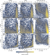 |
Fig. 5 Comparison of color-magnitude diagrams of unresolved sources selected from Rubin DP1 (top row), TRILEGAL simulation (middle row), and DES and DELVE data (bottom row). Each column corresponds to one of the Rubin DP1 fields (as designated in the top left corner of each panel). The color scale follows the probability density. While bin sizes are smaller in the rightmost column, the same color scale is shared between all panels. TRILEGAL, DELVE, and DES data have been selected so that the area of each field is equal to the approximate area covered by the corresponding DP1 fields. Recall that r < 24, star-galaxy separation and 0 < g − r < 1.4 selection criteria were applied. DELVE data contain only a few stars fainter than r≈22. We call attention to the deficit of faint (r > 22) blue stars (g − r < 0.6), compared to TRILEGAL simulation, in all three fields. |
2.4 Deficit of faint blue stars
The top row in Fig. 5 shows color-magnitude diagrams of unresolved sources selected from the three Rubin DP1 fields analyzed here. We select the plotted sample by limiting the apparent magnitude range to r < 247 and applied our star-galaxy separation method. The results of these cuts are listed in Table 1. Additionally, we restricted the color range to 0 < g − r < 1.4 While stellar counts generally increase with magnitude, m (for a uniform source distribution proportionally to 100.6m with the fiducial case of flat counts corresponding to a volume number density decreasing as 1/d3 with the distance, d) in all three fields, there is an indication of a deficit of blue stars (0.2 < g − r < 0.6) at r ~ 22–24, compared to stars with similar colors at brighter magnitudes.
The middle row in Fig. 5 shows color–magnitude diagrams predicted by TRILEGAL simulation. It is evident that predicted counts of faint blue stars exceed the observed counts. It is remarkable that TRILEGAL simulation reproduces the unusually well-defined separation of the disk and halo populations in the SV 95 −25 field: a diagonal paucity of stars extending from (r ~ 19, g − r ~ 0.2) to (r ~ 22, g − r ~ 0.6). Figures 6 and 7 provide a more quantitative visualization of this discrepancy by comparing the r-band counts in a narrow color range and the g − r color histograms for two faint slices of the r-band magnitude.
The region of the color–magnitude diagram where TRILEGAL overpredicts observed counts is dominated by halo stars. Motivated by SDSS results (Jurić et al. 2008; de Jong et al. 2010), TRILEGAL assumes the following halo number density profile for the halo component,
![Mathematical equation: $\[n(R, Z)=n_0\left(R^2+(Z / q)^2\right)^{-n / 2},\]$](/articles/aa/full_html/2026/03/aa57219-25/aa57219-25-eq2.png) (1)
(1)
where R and Z are galactocentric cylindrical coordinates, n0 is a population-specific constant, n = 2.75 is the halo power-law index, and q = 0.62 measures the halo oblateness (q = 1 for a spherical halo). This profile extends to a distance of 200 kpc, implying that counts for blue main sequence turn-off stars should remain high to about r ~ 26.5 (for more details, see Pieres et al. 2020). The implication of the observed deficit of faint blue stars is that the power-law index is much larger and the resulting profile much steeper at large galactocentric radii than observed by SDSS at brighter magnitudes. A more quantitative analysis is presented in Sect. 3.
DP1 is the very first release of Rubin photometric catalogs and all the results need to be interpreted with caution since it will take more time and more data to fully understand the behavior of image processing pipelines. For this reason, we compared Rubin data in these three fields to extant datasets (see Sect. 2.2). The bottom row in Fig. 5 shows color–magnitude diagrams constructed using DES and DELVE catalogs. While these datasets are a bit shallower than DP1, it is evident that they support our conclusion regarding the notable deficit of faint blue stars. Additionally, tests based on artificial source injection show that the source detection incompleteness at faint magnitudes cannot explain the blue star deficit and small, barely resolved galaxies do not show any deficit, but they do show a smooth increase in the counts in line with magnitude (NSF-DOE Vera C. Rubin Observatory 2025).
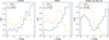 |
Fig. 6 Comparison of observed counts and TRILEGAL simulation using sources with 0.3 < g − r < 0.4, separately for each of the three DP1 fields, as marked at the top of each panel. Note: the TRILEGAL simulation predicts steep rise of counts for r < 21, which is not seen in Rubin data. |
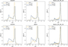 |
Fig. 7 Comparison of observed g − r color distributions and those predicted by TRILEGAL simulation for stars from two magnitude bins (top: 22 < r < 23, bottom: 23 < r < 24), separately for each of the three DP1 fields, as marked at the top of each panel. Note: the TRILEGAL simulation predicts significantly more blue turn-off stars. |
2.5 Distribution of stars in Rubin color–color diagrams and comparison with SDSS
For a more quantitative analysis of the stellar number density profile, estimates of stellar distances are required. Stellar distances can be estimated from broad-band colors using the Bayesian framework discussed in Palaversa et al. (2025). The stellar model color library required by the framework is derived from spectral energy distribution (SED) models using the SDSS photometric system. We note that when computing likelihoods they express all colors as functions of g − i color.
Although SDSS and Rubin photometric systems are similar, we can assess their differences by comparing the distribution of unresolved sources in Rubin’s color–color diagrams to stellar model color sequences from Palaversa et al. (2025, which are in excellent agreement with SDSS observations).
The largest discrepancy between SDSS and Rubin photometry for stars is seen in the g − r color distribution for red stars (M spectral type), as illustrated in Fig. 8. Based on a preliminary analysis of DP1 stars that also have SDSS photometry by M. Porter et al. (Rubin Technical Note RTN-099, in preparation), this difference in the g − r color comes primarily from the color term between the Rubin and SDSS g bandpasses, due to Rubin’s g bandpass red edge extending about 20 nm further to longer wavelengths compared to the SDSS g bandpass. The second largest color term is observed in the z band, with a strength of about one third of that in the g band. The color term in the r band is much smaller. Additionally, we systematically compare Rubin data and the stellar models used by photoD, available in the SDSS photometric system in Fig. 9.
Unfortunately, there are no available constraints for color terms in the Rubin u and y bands. The u band is especially important because it provides metallicity estimates, which in turn is needed for accurate distance estimates. Based on the top left panel in Fig. 9, it seems that there are no large offsets (say, larger than 0.1 mag) in the u − g color between the Rubin and SDSS systems. The models in the g − r versus u − g color–color diagram appear to be shifted upwards relative to Rubin data, but note that at faint magnitudes probed by Rubin the majority of blue stars is expected to belong to the low-metallicity halo population (Ivezić et al. 2008).
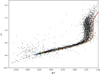 |
Fig. 8 Comparison of the distribution of unresolved sources from Rubin DP1 in the r − i vs. g − r color–color diagram (symbols) and stellar model color sequences from Palaversa et al. (2025), which are in excellent agreement with SDSS observations. The sequences are color-coded by metallicity (−2.5 < [Fe/H] < +0.5, linearly from blue to red), but in this color projection they are primarily degenerate (for more details see Fig. 3 in Palaversa et al. 2025). Note: M stars with r − i > 0.5 have a mean g − r color of ~1.3, while in the SDSS photometric system, this is g − r ~ 1.4. |
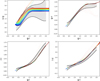 |
Fig. 9 Comparison of the color distributions of unresolved sources in Rubin DP1 (the shaded gray regions bounded by solid black lines represent ±2σ envelope around the median color in g − i bins) and stellar model color sequences from Palaversa et al. (2025). The sequences correspond to a 10 Gyr population are color-coded by metallicity; the full metallicity range is −2.5 < [Fe/H] < +0.5 and coded linearly from blue to red (for additional details, see Fig. 3 in Palaversa et al. 2025). |
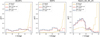 |
Fig. 10 Comparison of counts for selected subsamples using sources with 0.3 < g − r < 0.4, separately for each of the three DP1 fields, as marked at the top of each panel. Note: in the 22 < r < 23 magnitude range the effect of locus color cuts on the counts profile is negligible and remains minimal in the 23 < r < 24 magnitude range. |
2.6 Selection of main sequence stars using stellar locus selection
Given the stellar locus parametrization in Rubin photometric system shown in Fig. 9, the number of non-main sequence stars (e.g., white dwarfs), quasars, and unresolved galaxies in the unresolved sample can be further decreased by rejecting objects with colors that are not consistent with the 5D stellar color locus. We rejected all objects further than 2σ away from the median locus parametrized by the g − i color (i.e., outside the gray regions shown in Fig. 9. We note that red giant stars can also be found in the main stellar locus; however, their fraction is negligible at the faint magnitudes probed here. The rejected sources probably dominated by small unresolved galaxies and non-main sequence stars with varying colors (e.g. unresolved binary stars). We repeated the analysis with a 4σ rejection cut, but our results for the stellar number density profiles and metallicity distribution did not change appreciably.
In the context of our analysis of the stellar number density profile in the next section, it is important to ensure that this additional color-based rejection does not significantly alter the completeness of faint blue stars in the sample. As shown in Fig. 10, the effect of locus color cuts on the counts profile is negligible for r < 23 and remains minimal in the 23 < r < 24 magnitude range. The main effect and purpose of this selection step is to reject sources for which distance estimates would not be reliable in any case because their colors are inconsistent with the main sequence stellar locus.
2.7 Stellar photometric distance estimation
The Bayesian photoD framework compares observed colors to a library of model colors for various stellar populations. For main sequence stars, the models are parametrized by stellar luminosity (i.e., absolute magnitude, Mr), metallicity [Fe/H], and population age (of secondary importance when discussing data at high galactic latitudes as considered here). The models are augmented by the dust extinction (reddening) along the line of sight, parametrized by the extinction in the r band (Ar). The framework thus provides the best-fit values of Mr, [Fe/H], and Ar, along with their uncertainties.
Currently, there are two difficulties with applying this framework to the full Rubin DP1 dataset. First, the likelihood computation is very sensitive to discrepancies between observed and model colors. As we discussed above, photometric transformations for all Rubin bands are not available yet. In addition, priors derived from TRILEGAL simulations appear questionable at the faint end due to a deficit of observed faint blue stars compared to model predictions. In order to obtain (at least approximate) estimates of distances to halo stars, we instead followed Ivezić et al. (2008) and limited our analysis to blue stars near the main sequence turn-off point (g − i < 1). For these stars, Mr can be determined using an analytic expression for Mr as a function of the g − i color and [Fe/H], with the metallicity estimated using the u − g and g − r colors.
We estimated the absolute magnitudes using Eq. (A7) from Ivezić et al. (2008) and an updated expression for metallicity from Bond et al. (2010, Eq. (A1)). Based on an analysis of stars in globular clusters, Ivezić et al. (2008) estimated that the probable systematic errors in absolute magnitudes determined using these relations are about 0.1 mag, corresponding to 5% systematic distance errors (in addition to the 10–15% random distance errors). Since the DP1 dataset is at high galactic latitudes, we did not fit for Ar and, instead, we adopted the extinction values from the dust maps by Schlegel et al. (1998).
Based on the preliminary results (Porter et al. 2025, Rubin Technical Note RTN-099, in. prep), we transformed the Rubin’s LSSTComCam g − i color to SDSS-like g − i color using8
![Mathematical equation: $\[(g-i)_{S D S S}=1.065~(g-i)_{C o m C a m}+0.005,\]$](/articles/aa/full_html/2026/03/aa57219-25/aa57219-25-eq3.png) (2)
(2)
and analogously for the g − r color,
![Mathematical equation: $\[(g-r)_{S D S S}=1.058~(g-r)_{C o m C a m}+0.058~(r-i)_{C o m C a m}-0.002.\]$](/articles/aa/full_html/2026/03/aa57219-25/aa57219-25-eq4.png) (3)
(3)
In the g − i range relevant here (0.3 < g − i < 0.7), the resulting (g − i)SDSS color is about 0.03–0.05 mag redder than the (g − i)ComCam color, with a corresponding change of distance scale by about 1.5–2.5%. For the g − r color, the above transformation properly reproduces the mean SDSS g − r ~ 1.4 color for M stars (recalling Fig. 8).
The u band color term has the largest effect on distances via the impact of the u − g color on [Fe/H] estimates and, in turn, their impact on Mr estimates. For example, a systematic error in the u − g color of 0.02 mag induces a systematic [Fe/H] errors ranging from 0.02 dex for high-metallicity stars to 0.11 dex for low-metallicity halo stars (Ivezić et al. 2008). Unfortunately, the u band color term is currently not well known. Predictions based on stellar SED models (see Fig. 11) predict 0.15 mag around g − i = 0.5 relevant for blue stars considered below (due to the fact that the effective wavelength for the Rubin u bandpass is longer than for the SDSS u band). There is no overlap between DP1 fields and SDSS sky coverage. A preliminary performance analysis based on unpublished Rubin commissioning data of the COSMOS field with LSST Camera by the Rubin commissioning team supports the above model-based predictions for blue stars, but we note that the LSST Camera u band filter and LSSTComCam u band filter are physically different devices. Motivated by the model predictions and empirical comparison with the COSMOS field, we adopted the following simple corrections for blue stars with g − i ~ 0.5 considered below,
![Mathematical equation: $\[u_{SDSS}=u_{ComCam}+0.15.\]$](/articles/aa/full_html/2026/03/aa57219-25/aa57219-25-eq5.png) (4)
(4)
Its main effects are to shift metallicity distribution to higher values by about 0.4 dex and to make Mr brighter by 0.2–0.3 mag, resulting in larger distances by 10–15%. We return to this point and the effects of no u band correction in Sect. 4.
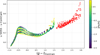 |
Fig. 11 Predictions for the color term between Rubin and SDSS u band magnitudes derived by integrating stellar model SED with photometric bandpasses. Symbols color-coded by metallicity (see the legend on the right) correspond to the Kurucz library models for main sequence stars with log(g) = 4.0, 4.5 and 5.0 (effective temperature changes along the locus). The red symbols correspond to models for cold stars from Allard et al. (2013). |
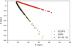 |
Fig. 12 Distribution of selected blue stars in galactocentric cylindrical coordinates for the three DP1 fields, as marked in the legend. The starting sample sizes are listed in the last column in Table 1. After further cuts (g − r < 0.6 and 4.0 < Mr < 5.5), the three subsamples include 378 (ECDFS), 387 (EDFS) and 3452 (SV 95 −25) stars. Note: the poor coverage of the R–Z plane with only three pencil beams. |
3 Analysis of the stellar halo number density and metallicity profiles
Here, we describe our construction and analysis of the resulting halo number density profiles and metallicity distributions. We only considered stars bluer than g − r = 0.60 to ensure reliable [Fe/H] estimates (Ivezić et al. 2008) and further limited them to a narrow absolute magnitude range, 4.0 < Mr < 5.5 (approximately corresponding to the 0.3 < g − i < 0.6 color range), to retain a good level of control over the selection effects at the faint end. Assuming a 100% completeness to the faint limit at r = 24, this subsample is complete to a distance modulus of 18.5 (50 kpc), with the completeness dropping to zero at a distance modulus of 20 (100 kpc). The distribution of a selected subsample in galactocentric cylindrical coordinates is shown in Fig. 12.
3.1 Halo number density profiles
Using stellar positions shown in Fig. 12, we were able to compute their number density profiles. For each field separately, we binned the distance modulus (see the left panels in Fig. 13) and for each bin, we computed the corresponding number density by dividing the stellar counts in a bin by the bin volume (easily computed as the volume difference of two cones defined by distance modulus bin boundaries). The resulting number density profiles are shown in the right panels in Fig. 13.
We performed an axially symmetric elliptical halo model fit (Eq. (1)) to data at galactocentric distances beyond 15 kpc, where halo counts dominate over the counts of disk stars. The best-fit profiles, with n ranging from 5 to 8, are much steeper than the SDSS-motivated q = 0.62 and n = 2.75 halo profile, measured at distances below 10 kpc and assumed in TRILEGAL simulations. Given the poor coverage of the R–Z plane with only three pencil beams, it is not possible to break the degeneracy between q and n. Thus, we provide best-fit n values for assumed values of q = 0.5 and q = 1, noting that the best-fit values of n should not be overinterpreted.
As a test of our analysis code, we repeated identical steps using simulated TRILEGAL catalog. As evident in Fig. 14, the q = 0.62 and n = 2.75 halo profile assumed in TRILEGAL simulations is faithfully reproduced for all three sky directions. It is interesting to compare the bottom-left panels in Figs. 13 and 14. The paucity of predicted halo stars for distance modulus values larger than 17 is clearly seen (and directly related to the results shown in Figs. 6 and 7).
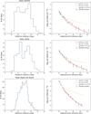 |
Fig. 13 Distance modulus distribution (left) and stellar number density profile (right) for the three Rubin DP1 fields analyzed in this study shown in each row. Note: the sample distance modulus completeness limit is 18.5 and, thus, the steeply decreasing right edge of the distance modulus distributions is a real effect and not a selection effect. In the right column, data are shown as symbols with Poisson uncertainties and lines are axially symmetric elliptical halo models (Eq. (1)), with the corresponding n and q parameters listed in the legend (see text). Note: the data display much steeper profiles than the SDSS-motivated q = 0.62 and n = 2.75 halo profile assumed in TRILEGAL simulations. |
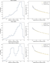 |
Fig. 14 Same as Fig. 13, except that the TRILEGAL simulation is used instead of Rubin DP1 data. Note: the q = 0.62 and n = 2.75 halo profile assumed in simulations is faithfully reproduced (although it cannot be distinguished from the canonical spherical 1/r3 profile due to sparse coverage of the R–Z plane). |
3.2 Halo metallicity distributions
The metallicity distribution of selected blue stars is shown in Fig. 15. The distributions in the ~20 kpc galactocentric distance slice are consistent with expectations for halo stars (the halo metallicity distribution for stars within 10 kpc measured by SDSS is centered on [Fe/H] = −1.5; Ivezić et al. 2008). The 10 kpc bin is more representative of high-metallicity disk stars. For comparison (and again as a test of our analysis code), Fig. 16 shows results obtained with the simulated TRILEGAL catalog. As expected, the metallicity distribution in the 20 kpc bin is consistent with the assumed distribution centered on [Fe/H] = −1.5, while the 10 kpc bin seems dominated by higher-metallicity disk stars, similarly to what is seen in the DP1 distributions.
4 Discussion and conclusions
Distances to stars are a crucial ingredient in our quest to better understand the formation and evolution of the Milky Way galaxy. Anticipating photometric catalogs with tens of billions of stars from Rubin’s LSST, we investigated the utility of Rubin’s DP1 catalogs for estimating stellar number density profile in the Milky Way halo. Although DP1 includes only three very small fields, it has nevertheless enabled several important aspects of the results presented here.
We found a notable deficit of faint (r > 22) blue main sequence stars compared to cutting-edge TRILEGAL simulations. This finding is supported by extant data from DES and DELVE surveys, although they do not share the same confidence level for each of the three fields (particularly the SV 95–25 field in the 22 < r < 24 regime). This discrepancy is interpreted as a signature of a steeper halo number density profile at galactocentric distances 10–50 kpc than the SDSS-motivated 1/r2.75 profile assumed in TRILEGAL simulations. This interpretation is consistent with earlier suggestions based on observations of more luminous, but much less numerous, evolved stellar populations, and a few pencil beam surveys of blue main sequence stars in the northern sky: at about 20–30 kpc, the profile slope changes from about n ~ 2–3 to about n ~ 4–5 (see Fig. 7 in Medina et al. 2024 for a visual summary of results from many studies). We were unable to break the degeneracy between the oblateness parameter (q) and the exponent, n, given only three pencil beam constraints from DP1 dataset. For this reason, the measured exponents, n, should be interpreted with caution (for a related discussion, see Pila-Díez et al. 2015).
Our metallicity results are in agreement with the expectations for a halo distribution centered on [Fe/H] = −1.5, as measured by SDSS out to 10 kpc. Nevertheless, the applied u band color term (Eq. (4)) of 0.15 mag is probably uncertain to about 0.05 mag. As a result of that uncertainty, there are likely systematic errors in observed [Fe/H] distributions (shifts along the abscissa) of about 0.2 dex (and implied distance scale changes of about 10%). We note that uncertainty in the u band correction has no discernible effect on the halo profile shape since it is well described by a power law. Therefore, we cannot exclude a halo metallicity gradient of up to about 0.2 dex between galactocentric distances of 10 kpc and 50 kpc.
As Rubin collects more data with the much larger LSST Camera (compared to the LSSTComCam) in sky regions with SDSS coverage, it will be possible to derive robust and precise photometric transformations between the Rubin and SDSS photometric systems (e.g., the equatorial SDSS Stripe 82 region would be ideal for such studies; for details see Thanjavur et al. 2021). In addition, the LSST photometric throughput will be well measured and can be used to compute colors from stellar SED models without an intermediate reference to the SDSS system. With improved stellar model colors and with adequate adjustments to stellar population models, such as TRILEGAL, used for priors, it will be possible to deploy the full Bayesian framework described in Palaversa et al. (2025).
Ultimately, Rubin’s LSST will cover half the sky, an area more than 10 000 times larger than, for example, the ECDFS field analyzed here and down to a similar depth. As one among many benefits of a large sky coverage, LSST data will break the q − n degeneracy when fitting halo number density profiles. Further anticipated improvements in this context brought about by the ten-year LSST dataset are discussed in detail by Palaversa et al. (2025). We conclude that the results presented here bode well for future explorations of the Milky Way with LSST.
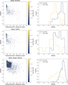 |
Fig. 15 Each row shows the variation of stellar metallicity with galactocentric distance (left) and metallicity distribution in two slices of distance (right), as marked in the legend. See text for details. |
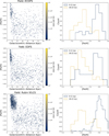 |
Fig. 16 Analogous to Fig. 15, except that the TRILEGAL simulation is used instead of Rubin DP1 data. Note: the metallicity distribution in the more distant bin dominated by halo stars is consistent with a distribution centered on [Fe/H] = −1.5 assumed in simulations. |
Acknowledgements
This work was supported by the Croatian Science Foundation under the project number IP-2025-02-1942 and has been financed within the Tenure Track Pilot Programme of the Croatian Science Foundation and the Ecole Polytechnique Fédérale de Lausanne and the Project TTP-2018-07-1171 “Mining the Variable Sky”, with the funds of the Croatian-Swiss Research Programme. This material is based upon work supported in part by the National Science Foundation through Cooperative Agreements AST-1258333 and AST-2241526 and Cooperative Support Agreements AST-1202910 and 2211468 managed by the Association of Universities for Research in Astronomy (AURA), and the Department of Energy under Contract No. DE-AC02-76SF00515 with the SLAC National Accelerator Laboratory managed by Stanford University. Additional Rubin Observatory funding comes from private donations, grants to universities, and in-kind support from LSST-DA Institutional Members. L.P. acknowledges support from LSST-DA through grant 2024-SFF-LFI-08-Palaversa. This work was conducted as part of a LINCC Frameworks Incubator. LINCC Frameworks is supported by Schmidt Sciences. W.B., D.B, A. J. C., N.C., S.C., M.D., D.J., O.L., K.M., A.I.M., and S.M., are supported by Schmidt Sciences. Ž.I, M.J. and N.C. acknowledge support from the DiRAC Institute in the Department of Astronomy at the University of Washington. M.J. and N.C. would also like to acknowledge support by the National Science Foundation under Grant No. AST-2003196. The DiRAC Institute is supported through generous gifts from the Charles and Lisa Simonyi Fund for Arts and Sciences and the Washington Research Foundation. Funding for the SDSS9 and SDSS-II9 has been provided by the Alfred P. Sloan Foundation, the Participating Institutions, the National Science Foundation, the U.S. Department of Energy, the National Aeronautics and Space Administration, the Japanese Monbukagakusho, the Max Planck Society, and the Higher Education Funding Council for England. G.P., L.G., M.T. and S.Z. acknowledge support from project “SPICE4LSST – Adding incompleteness and crowding errors to the LSST Data Releases” (INAF Large Grant 2024). LG and SZ acknowledge support from “Population synthesis with rotating stars: a necessary upgrade” (INAF Theory Grant 2022). MT and GP acknowledge financial support by the European Union – NextGenerationEU and by the University of Padua under the 2023 STARS Grants@Unipd programme (“CONVERGENCE: CONstraining the Variability of Evolved Red Giants for ENhancing the Comprehension of Exoplanets”). This work has made use of data from the European Space Agency (ESA) mission Gaia10, processed by the Gaia Data Processing and Analysis Consortium (DPAC11). Funding for the DPAC has been provided by national institutions, in particular, the institutions participating in the Gaia Multilateral Agreement. Facilities. Vera C. Rubin Observatory, Gaia, Sloan Digital Sky Survey, Blanco Telescope and DECam. Software. Astropy(Astropy Collaboration 2013, 2018), AstroML (VanderPlas et al. 2012), HATS (Caplar et al. 2025), Jupyter (Kluyver et al. 2016), LSDB (Caplar et al. 2025), Matplotlib (Hunter 2007), Numpy (Oliphant 2006), Scipy (Virtanen et al. 2020), Seaborn (Waskom 2021), Pandas McKinney (2010), Python (Van Rossum & Drake 2009).
References
- Abbott, T. M. C., Adamów, M., Aguena, M., et al. 2021, ApJS, 255, 20 [NASA ADS] [CrossRef] [Google Scholar]
- Allard, F., Homeier, D., Freytag, B., Schaffenberger, W., & Rajpurohit, A. S. 2013, Mem. Soc. Astron. Ital. Suppl., 24, 128 [Google Scholar]
- Astropy Collaboration (Robitaille, T. P., et al.) 2013, A&A, 558, A33 [NASA ADS] [CrossRef] [EDP Sciences] [Google Scholar]
- Astropy Collaboration (Price-Whelan, A. M., et al.) 2018, AJ, 156, 123 [Google Scholar]
- Bahcall, J. N. 1986, ARA&A, 24, 577 [Google Scholar]
- Bianco, F. B., Ivezić, Ž., Jones, R. L., et al. 2022, ApJS, 258, 1 [NASA ADS] [CrossRef] [Google Scholar]
- Bond, N. A., Ivezić, Ž., Sesar, B., et al. 2010, ApJ, 716, 1 [NASA ADS] [CrossRef] [Google Scholar]
- Caplar, N., Beebe, W., Branton, D., et al. 2025, arXiv e-prints [arXiv:2501.02103] [Google Scholar]
- Carlin, J. L., Ferguson, P. S., Vivas, A. K., Caplar, N., & Malanchev, K. 2025, RNAAS, 9, 161 [Google Scholar]
- Choi, Y., Olsen, K. A. G., Carlin, J. L., et al. 2025, ApJ, 992, 47 [Google Scholar]
- Dal Tio, P., Pastorelli, G., Mazzi, A., et al. 2022, ApJS, 262, 22 [NASA ADS] [CrossRef] [Google Scholar]
- de Jong, J. T. A., Yanny, B., Rix, H.-W., et al. 2010, ApJ, 714, 663 [NASA ADS] [CrossRef] [Google Scholar]
- Deason, A. J., Belokurov, V., Koposov, S. E., & Rockosi, C. M. 2014, ApJ, 787, 30 [NASA ADS] [CrossRef] [Google Scholar]
- Drlica-Wagner, A., Ferguson, P. S., Adamów, M., et al. 2022, ApJS, 261, 38 [NASA ADS] [CrossRef] [Google Scholar]
- Faccioli, L., Smith, M. C., Yuan, H. B., et al. 2014, ApJ, 788, 105 [Google Scholar]
- Feng, Y., Guhathakurta, P., Peng, E. W., et al. 2024, ApJ, 966, 159 [Google Scholar]
- Fukushima, T., Chiba, M., Tanaka, M., et al. 2025, PASJ, 77, 178 [Google Scholar]
- Han, J. J., Conroy, C., Johnson, B. D., et al. 2022, AJ, 164, 249 [NASA ADS] [CrossRef] [Google Scholar]
- Hunter, J. D. 2007, Comput. Sci. Eng., 9, 90 [NASA ADS] [CrossRef] [Google Scholar]
- Ivezić, Ž., Sesar, B., Jurić, M., et al. 2008, ApJ, 684, 287 [Google Scholar]
- Ivezić, Ž., Beers, T. C., & Jurić, M. 2012, ARA&A, 50, 251 [Google Scholar]
- Ivezić, Ž., Kahn, S. M., Tyson, J. A., et al. 2019, ApJ, 873, 111 [Google Scholar]
- Jurić, M., Ivezić, Ž., Brooks, A., et al. 2008, ApJ, 673, 864 [Google Scholar]
- Kluyver, T., Ragan-Kelley, B., Pérez, F., et al. 2016, in Positioning and Power in Academic Publishing: Players, Agents and Agendas, eds. F. Loizides, & B. Schmidt (IOS Press), 87 [Google Scholar]
- Malanchev, K., DeLucchi, M., Caplar, N., et al. 2025, arXiv e-prints [arXiv:2506.23955] [Google Scholar]
- McKinney, W. 2010, in Proceedings of the 9th Python in Science Conference, eds. S. van der Walt, & J. Millman, 51 [Google Scholar]
- Medina, G. E., Muñoz, R. R., Carlin, J. L., et al. 2024, MNRAS, 531, 4762 [NASA ADS] [CrossRef] [Google Scholar]
- NSF-DOE Vera C. Rubin Observatory 2025, Legacy Survey of Space and Time Data Preview 1 [Data set] [Google Scholar]
- NSF-DOE Vera C. Rubin Observatory 2025, The Vera C. Rubin Observatory Data Preview 1, Technical Note RTN-095, Vera C. Rubin Observatory [Google Scholar]
- Oliphant, T. E. 2006, A Guide to NumPy, 1 (Trelgol Publishing USA) [Google Scholar]
- Palaversa, L., Ivezić, Ž., Caplar, N., et al. 2025, AJ, 169, 119 [Google Scholar]
- Pieres, A., Girardi, L., Balbinot, E., et al. 2020, MNRAS, 497, 1547 [NASA ADS] [CrossRef] [Google Scholar]
- Pila-Díez, B., de Jong, J. T. A., Kuijken, K., van der Burg, R. F. J., & Hoekstra, H. 2015, A&A, 579, A38 [NASA ADS] [CrossRef] [EDP Sciences] [Google Scholar]
- Porter, M. N., Tucker, D. L., Smith, J. A., & Adair, C. L. 2025, Photometric Transformation Relations for the LSST Data Preview 1, Technical Note RTN-099, Vera C. Rubin Observatory [Google Scholar]
- Schlegel, D. J., Finkbeiner, D. P., & Davis, M. 1998, ApJ, 500, 525 [Google Scholar]
- Sesar, B., Jurić, M., & Ivezić, Ž. 2011, ApJ, 731, 4 [CrossRef] [Google Scholar]
- SLAC & NSF-DOE Vera C. Rubin Observatory 2024, LSST Commissioning Camera [Google Scholar]
- Slater, C. T., Ivezić, Ž., & Lupton, R. H. 2020, AJ, 159, 65 [Google Scholar]
- Stringer, K. M., Drlica-Wagner, A., Macri, L., et al. 2021, ApJ, 911, 109 [Google Scholar]
- Thanjavur, K., Ivezić, Ž., Allam, S. S., et al. 2021, MNRAS, 505, 5941 [NASA ADS] [CrossRef] [Google Scholar]
- Van Rossum, G., & Drake, F. L. 2009, Python 3 Reference Manual (Scotts Valley, CA: CreateSpace) [Google Scholar]
- VanderPlas, J., Connolly, A. J., Ivezić, Ž., & Gray, A. 2012, in Proceedings of Conference on Intelligent Data Understanding (CIDU), 47 [Google Scholar]
- Virtanen, P., Gommers, R., Oliphant, T. E., et al. 2020, Nat. Methods, 17, 261 [Google Scholar]
- Wainer, T. M., Davenport, J. R. A., Bellm, E. C., et al. 2025, RNAAS, 9, 171 [Google Scholar]
- Waskom, M. L. 2021, J. Open Source Softw., 6, 3021 [CrossRef] [Google Scholar]
- Wetterer, C. J., & McGraw, J. T. 1996, AJ, 112, 1046 [Google Scholar]
- Yu, F., Li, T. S., Speagle, J. S., et al. 2024, ApJ, 975, 81 [Google Scholar]
Flux derived from using the PSF model as a weight function and measured on band b.
Exposures in the u-band are 38 seconds long, as the sky background noise is more easily dominated by read noise.
At the faint magnitudes probed here, many galaxies and quasars are unresolved in ground-based seeing (here in the range 1.0–1.3 arcsec). In addition, even some stars may appear resolved (for example, stars with circumstellar shells and close binary stars). Therefore, “star-galaxy separation” really refers to the separation of unresolved and resolved sources. For more details, please see Slater et al. (2020).
The CModel (or “composite model”) flux is computed with a best-fit source surface brightness profile, while PSF flux is computed with the point spread function profile. For extended sources, the PSF flux is biased low. For more details, see Slater et al. (2020).
Where there is no evidence of appreciable contamination by galaxies (recall Fig. 4).
Both valid in the range 0.2 < (g − i)ComCam < 3.0).
All Tables
All Figures
|
Fig. 1 Sky coverage of Rubin DP1 dataset. The seven LSSTComCam fields are shown as yellow dots (with names) in the context of the LSST’s planned regions: North Ecliptic Spur (purple), South Celestial Pole (yellow), the dusty plane, the Galactic Plane and Magellanic Clouds (brown and green), and low-dust-extinction regions of the Wide-Fast-Deep (blue) program. Here, we analyze data from three fields: ECDFS, EDFS, and Rubin SV 95 −25. |
| In the text | |
|
Fig. 2 Difference between the PSF (point spread function) magnitude and the CModel magnitude in the gri bands, and the mean gri value (bottom right) vs. magnitude for the ECDFS field (analogous to Fig. 1 from Slater et al. 2020). The colormap encodes the number of stars per bin. The bimodal distribution of stars and galaxies (more precisely, unresolved and resolved sources) is evident. |
| In the text | |
|
Fig. 3 Same as Fig. 2, except that the abscissa is zoomed in on, and the left panels show the u and y band diagrams, respectively. The two vertical lines in the bottom right panel show the separation boundary between unresolved and resolved sources (dashed at 0.016 mag: Rubin default value for single-band classification; solid at 0.04 mag: adopted here for the mean gri values and designed to ensure stellar completeness to faint magnitude limits). |
| In the text | |
|
Fig. 4 Comparison of color–magnitude diagrams of unresolved (top) and resolved (bottom) sources selected from Rubin DP1 fields ECDFS (left) and SV 95 −25 (right). Note: low fractions of unresolved sources (approximately 8% in the ECDFS field and 24% in the SV 95 −25 field, for r < 25). |
| In the text | |
|
Fig. 5 Comparison of color-magnitude diagrams of unresolved sources selected from Rubin DP1 (top row), TRILEGAL simulation (middle row), and DES and DELVE data (bottom row). Each column corresponds to one of the Rubin DP1 fields (as designated in the top left corner of each panel). The color scale follows the probability density. While bin sizes are smaller in the rightmost column, the same color scale is shared between all panels. TRILEGAL, DELVE, and DES data have been selected so that the area of each field is equal to the approximate area covered by the corresponding DP1 fields. Recall that r < 24, star-galaxy separation and 0 < g − r < 1.4 selection criteria were applied. DELVE data contain only a few stars fainter than r≈22. We call attention to the deficit of faint (r > 22) blue stars (g − r < 0.6), compared to TRILEGAL simulation, in all three fields. |
| In the text | |
|
Fig. 6 Comparison of observed counts and TRILEGAL simulation using sources with 0.3 < g − r < 0.4, separately for each of the three DP1 fields, as marked at the top of each panel. Note: the TRILEGAL simulation predicts steep rise of counts for r < 21, which is not seen in Rubin data. |
| In the text | |
|
Fig. 7 Comparison of observed g − r color distributions and those predicted by TRILEGAL simulation for stars from two magnitude bins (top: 22 < r < 23, bottom: 23 < r < 24), separately for each of the three DP1 fields, as marked at the top of each panel. Note: the TRILEGAL simulation predicts significantly more blue turn-off stars. |
| In the text | |
|
Fig. 8 Comparison of the distribution of unresolved sources from Rubin DP1 in the r − i vs. g − r color–color diagram (symbols) and stellar model color sequences from Palaversa et al. (2025), which are in excellent agreement with SDSS observations. The sequences are color-coded by metallicity (−2.5 < [Fe/H] < +0.5, linearly from blue to red), but in this color projection they are primarily degenerate (for more details see Fig. 3 in Palaversa et al. 2025). Note: M stars with r − i > 0.5 have a mean g − r color of ~1.3, while in the SDSS photometric system, this is g − r ~ 1.4. |
| In the text | |
|
Fig. 9 Comparison of the color distributions of unresolved sources in Rubin DP1 (the shaded gray regions bounded by solid black lines represent ±2σ envelope around the median color in g − i bins) and stellar model color sequences from Palaversa et al. (2025). The sequences correspond to a 10 Gyr population are color-coded by metallicity; the full metallicity range is −2.5 < [Fe/H] < +0.5 and coded linearly from blue to red (for additional details, see Fig. 3 in Palaversa et al. 2025). |
| In the text | |
|
Fig. 10 Comparison of counts for selected subsamples using sources with 0.3 < g − r < 0.4, separately for each of the three DP1 fields, as marked at the top of each panel. Note: in the 22 < r < 23 magnitude range the effect of locus color cuts on the counts profile is negligible and remains minimal in the 23 < r < 24 magnitude range. |
| In the text | |
|
Fig. 11 Predictions for the color term between Rubin and SDSS u band magnitudes derived by integrating stellar model SED with photometric bandpasses. Symbols color-coded by metallicity (see the legend on the right) correspond to the Kurucz library models for main sequence stars with log(g) = 4.0, 4.5 and 5.0 (effective temperature changes along the locus). The red symbols correspond to models for cold stars from Allard et al. (2013). |
| In the text | |
|
Fig. 12 Distribution of selected blue stars in galactocentric cylindrical coordinates for the three DP1 fields, as marked in the legend. The starting sample sizes are listed in the last column in Table 1. After further cuts (g − r < 0.6 and 4.0 < Mr < 5.5), the three subsamples include 378 (ECDFS), 387 (EDFS) and 3452 (SV 95 −25) stars. Note: the poor coverage of the R–Z plane with only three pencil beams. |
| In the text | |
|
Fig. 13 Distance modulus distribution (left) and stellar number density profile (right) for the three Rubin DP1 fields analyzed in this study shown in each row. Note: the sample distance modulus completeness limit is 18.5 and, thus, the steeply decreasing right edge of the distance modulus distributions is a real effect and not a selection effect. In the right column, data are shown as symbols with Poisson uncertainties and lines are axially symmetric elliptical halo models (Eq. (1)), with the corresponding n and q parameters listed in the legend (see text). Note: the data display much steeper profiles than the SDSS-motivated q = 0.62 and n = 2.75 halo profile assumed in TRILEGAL simulations. |
| In the text | |
|
Fig. 14 Same as Fig. 13, except that the TRILEGAL simulation is used instead of Rubin DP1 data. Note: the q = 0.62 and n = 2.75 halo profile assumed in simulations is faithfully reproduced (although it cannot be distinguished from the canonical spherical 1/r3 profile due to sparse coverage of the R–Z plane). |
| In the text | |
|
Fig. 15 Each row shows the variation of stellar metallicity with galactocentric distance (left) and metallicity distribution in two slices of distance (right), as marked in the legend. See text for details. |
| In the text | |
|
Fig. 16 Analogous to Fig. 15, except that the TRILEGAL simulation is used instead of Rubin DP1 data. Note: the metallicity distribution in the more distant bin dominated by halo stars is consistent with a distribution centered on [Fe/H] = −1.5 assumed in simulations. |
| In the text | |
Current usage metrics show cumulative count of Article Views (full-text article views including HTML views, PDF and ePub downloads, according to the available data) and Abstracts Views on Vision4Press platform.
Data correspond to usage on the plateform after 2015. The current usage metrics is available 48-96 hours after online publication and is updated daily on week days.
Initial download of the metrics may take a while.