| Issue |
A&A
Volume 707, March 2026
|
|
|---|---|---|
| Article Number | A358 | |
| Number of page(s) | 13 | |
| Section | Interstellar and circumstellar matter | |
| DOI | https://doi.org/10.1051/0004-6361/202557277 | |
| Published online | 20 March 2026 | |
The 3D time evolution of the dust size distribution in protostellar envelopes
1
Université Paris-Saclay, Université Paris Cité, CEA, CNRS, AIM,
91191
Gif-sur-Yvette,
France
2
Institute of Space Sciences (ICE), CSIC, Campus UAB, Carrer de Can Magrans s/n,
08193
Barcelona,
Spain
3
ICREA,
Pg. Lluís Companys 23,
Barcelona,
Spain
★ Corresponding author: This email address is being protected from spambots. You need JavaScript enabled to view it.
Received:
16
September
2025
Accepted:
11
January
2026
Abstract
Context. Dust plays a fundamental role during protostellar collapse and disk and planet formation. Recent observations suggest that efficient dust growth can begin early in the protostellar envelopes, potentially even before the formation of the disk. Three-dimensional models of protostellar evolution that address multi-size dust growth, gas and dust dynamics, and magnetohydrodynamics (MHD) are required to characterize the dust evolution in the embedded stages of star formation.
Aims. We aim to establish a new framework for dust evolution models that follow in 3D the dust size distribution in both time and space, i.e., MHD models that describe the formation and evolution of star–disk systems at low numerical cost.
Methods. We coupled the COALA dust evolution module that uses the Smoluchowski equations to RAMSES numerical computations, performing the first 3D MHD simulation of protostellar collapse that simultaneously includes polydisperse dust growth modeled by the Smoluchowski equation and dust dynamics in the terminal velocity approximation.
Results. We note that, locally in the protostellar collapse, the dust size distribution deviates significantly from the Mathis–Rumpl–Nordsieck (MRN) distribution due to dust growth. Ice-coated micron-sized grains can rapidly grow in the envelope and survive by not entering the fragmentation regime. The evolution of the dust size distribution is highly inhomogeneous due to the turbulent nature of the collapse and the development of favorable locations, such as outflow cavity walls, which locally enhance the dust-to-gas ratio.
Conclusions. We analyzed the first 3D non-ideal MHD simulations that self-consistently account for dust dynamics and growth during the protostellar stage. Very early in the lifetime of a young embedded protostar, micron-sized grains can grow, and locally the dust size distribution deviates from the initial MRN shape. This new numerical method opens the possibility of treating gas and dust dynamics with dust growth simultaneously in 3D simulations at a low numerical cost for several astrophysical environments.
Key words: methods: numerical / protoplanetary disks / stars: formation / stars: protostars / dust, extinction / evolution
© The Authors 2026
 Open Access article, published by EDP Sciences, under the terms of the Creative Commons Attribution License (https://creativecommons.org/licenses/by/4.0), which permits unrestricted use, distribution, and reproduction in any medium, provided the original work is properly cited.
This article is published in open access under the Subscribe to Open model. This email address is being protected from spambots. You need JavaScript enabled to view it. to support open access publication.
1 Introduction
The formation and early evolution of dust grains in young stellar systems represent a critical yet poorly understood component of star and planet formation processes. While dust grains constitute only ~1% of the mass of the interstellar medium (ISM), they fundamentally influence protostellar evolution through their roles in radiative cooling, chemistry catalysis, and magnetic field coupling (Draine 2003; Zhao et al. 2016; Lebreuilly et al. 2023b; Vallucci-Goy et al. 2024).
Observations of the dust thermal emission at different frequencies allow us to measure the dust emissivity, β, a quantity that is key to computing dust masses from dust emission but is also widely used to measure the mean dust grain size in astrophysical environments and discuss, for example, dust evolution from submicronic solid particles toward pebbles and the formation of planetary systems (Testi et al. 2014; Birnstiel 2024). Some pilot observational studies suggested that young (<1 Myr old) disks show a dust emissivity evolution that is consistent with an increase in the mean dust grain size (Kwon et al. 2009; Miotello et al. 2014). More recently, observations have revealed compelling evidence that dust evolution is more complex than expected and may begin earlier than previously assumed (maybe even starting during the pre-stellar phase), which challenges traditional models that assume significant grain growth only occurred in disks. For example, Dartois et al. (2024) modeled the CO2 ice band observed by JWST in two lines of sight in a dense cloud (N(H) of ~1–2 × 1023 cm−2, Av > 60). They interpret the extended blue wing of this band as an excess of scattered light and conclude that, to explain this spectral feature, a fair fraction of the dust mass must be in grains of ~1 micrometer in size. At longer wavelengths, observational studies of the Taurus B211/B213 star-forming filament have shown a systematic decrease in the dust emissivity index (β) from β ≈ 2 in pre-stellar cores at scales of ~10 000 au to β < 1 toward protostellar envelopes (Ysard et al. 2013; Bracco et al. 2017). Low dust emissivities, β, have also been observed in the inner envelopes of embedded protostars in high-angular-resolution studies of the millimeter dust emission (Galametz et al. 2019; Cacciapuoti et al. 2023). All together, these studies reveal a variety of dust optical properties. However, the lowest dust emissivity (β) values have only so far been reproduced by including large dust grains (>100 μm), which suggests that efficient grain aggregation could begin in dense cores and envelopes long before dust grains have entered the disk environment.
Improving our modeling of the dust size distribution during the star-formation sequence requires us to address the magnetohydrodynamics (MHD) of gas and dust mixtures simultaneously with a full treatment of dust evolution. State-of-the-art dust evolution models employ distinct numerical strategies to balance computational feasibility with physical fidelity. Three-dimensional simulations are required to capture asymmetries in the evolution of the collapse. However, they are challenging and therefore often adopt a monodisperse or bi-disperse1 approximation to resolve dust growth (Vorobyov & Elbakyan 2019; Elbakyan et al. 2020; Tsukamoto et al. 2021; Vorobyov et al. 2024, 2025) or do not include dust-gas differential dynamics (Bate 2022; Marchand et al. 2023). We note the very recent effort of Bate et al. (2025) to couple dust dynamics with a full treatment of dust evolution with the Smoluchowski equation. They employed methods for collapse calculation that resemble those presented in this article but using Smooth Particle Hydrodynamic (SPH) methods. Conversely, several codes have been developed to solve the Smoluchowski equation across a wide span of grains size with the gas and dust dynamics in 1D, such as DustPy (Stammler & Birnstiel 2022) and shark (Lebreuilly et al. 2023b; Vallucci-Goy et al. 2024), or in 2D, such as LA-COMPASS (Drążkowska et al. 2019; Li et al. 2020; Ho et al. 2024) and CUDISC (Robinson et al. 2024), with a significant numerical cost. Recent efforts like the TriPoD framework (Pfeil et al. 2024) aim to reduce this numerical cost by embedding parameterized size distributions in 2D hydrodynamic grids, although challenges persist in reconciling growth timescales with dynamical environments. However, incorporating accurate numerical solutions to the Smoluchowski equation in 3D multi-physics hydrodynamic simulations is out of reach with the mentioned algorithms. This numerical challenge requires a new algorithm to efficiently solve the Smoluchowski equation. Thanks to the newly developed COALA code, it is now possible to fully solve the Smoluchowski equation for a wide range of grain sizes on the fly in 3D simulations that also follow dust dynamics. In the present study, by coupling COALA to the adaptive mesh-refinement code RAMSES, we ran simulations beyond the current state of the art that follow nonideal MHD protostellar collapses with a full solving of the Smoluchowski equation together with a treatment of dust dynamics in the terminal velocity approximation.
2 Methods
In this work, we performed numerical 3D MHD simulations of protostellar collapses using the RAMSES code (Teyssier 2002). In particular, we employed its extension to nonideal MHD (Masson et al. 2012). We followed the evolution of a gravitationally unstable pre-stellar core of 2.5 M⊙ with an initial radius of ~8000 au2 and an initial turbulent Mach 0 or 1 (denoted ℳ0 and ℳ1). Initial conditions were similar to those in the models presented in Maury et al. (2019) and Valdivia et al. (2022). The temperature of the cloud was computed assuming a barotropic equation of state as per Lebreuilly et al. (2020), which assumes isothermality below 10−13 g cm−3 and adiabaticity with an adiabatic index of 5/3 above. We used the adaptive-mesh refinement capability of RAMSES to follow the gravitational collapse. The coarse grid had a resolution of 1100 au and was refined by imposing at least ten points per Jeans length to avoid artificial fragmentation (Truelove et al. 1997); it reached a minimum cell size of 4.3 au in the densest regions.
2.1 Dust growth with COALA
We incorporated a full treatment of the dust coagulation by solving the Smoluchowski equation for single-composition spherical grains in the conservative form on the fly (Tanaka et al. 1996) using the COALA code (Lombart & Laibe 2021). Assuming a mass range [mmin, mmax] for the dust grains, the equation is written as
}{\partial m}=0, \\& F_{\text {growth}}[g](m, t) \\& \equiv \int_{m_{\min }}^m \int_{m-m_1+m_{\min }}^{m_{\max }-m_1+m_{\min }} \frac{K\left(m_1, m_2\right)}{m_2} g\left(m_1, t\right) g\left(m_2, t\right) \mathrm{d} m_2 \mathrm{d} m_1,\end{aligned}\]$](/articles/aa/full_html/2026/03/aa57277-25/aa57277-25-eq1.png) (1)
(1)
where m ∈ [mmin, mmax] is the mass of dust grains, g(m, t) is the dust mass distribution, and K(m1, m2) is the collision kernel between the two grains of masses m1 and m2. We used the ballistic kernel K(m1, m2) = σ(m1, m2) Δv(m1, m2), where σ is the collisional cross section and Δv is the differential velocity between grains. In this study, the sources of grain-grain differential velocities are Brownian motion, hydrodynamical drift, and gas turbulence (see details in Appendix A). We used the high accuracy of the COALA code to follow the evolution of the dust size distribution with a low number of dust size bins. The time solver implemented in COALA is a strong stability preserving Runge-Kutta third order (Gottlieb et al. 2009). In each spatial cell, we used 𝒩 > 1 dust species for which the set of dust mass density {ρk}1≤k≤𝒩 defines the dust size distribution. The dust mass distribution (g) in Eq. (1) is linked to ρk such that
![Mathematical equation: $\[\rho_k=\int_{I_k} g(m, t) \mathrm{d} m,\]$](/articles/aa/full_html/2026/03/aa57277-25/aa57277-25-eq2.png) (2)
(2)
with Ii the size of bin k. In this study, the code COALA gives the evolution of the mean value of the function g, noted ![Mathematical equation: $\[\bar{g}\]$](/articles/aa/full_html/2026/03/aa57277-25/aa57277-25-eq3.png) , which means that the piecewise constant approximation is used. Therefore, the relation between ρk and
, which means that the piecewise constant approximation is used. Therefore, the relation between ρk and ![Mathematical equation: $\[\bar{g}_{k}\]$](/articles/aa/full_html/2026/03/aa57277-25/aa57277-25-eq4.png) is directly obtained,
is directly obtained, ![Mathematical equation: $\[\bar{g}_{k}= \rho_{k} / \Delta m_{k}\]$](/articles/aa/full_html/2026/03/aa57277-25/aa57277-25-eq5.png) . The accuracy of the approximation of g depends on the number of dust bins, 𝒩. In Appendix B, COALA is benchmarked with exact solutions in the setup given in Sect. 2.4.
. The accuracy of the approximation of g depends on the number of dust bins, 𝒩. In Appendix B, COALA is benchmarked with exact solutions in the setup given in Sect. 2.4.
2.2 Dust dynamics with RAMSES
The dust dynamics was treated by the terminal velocity approximation solver of Lebreuilly et al. (2019). In short, this approach considers dust species as separate phases in a monofluid composed of the full gas-dust mixture with density ρ and velocity v. Each dust phase (k) of density ρk required us to solve a mass conservation equation with a velocity vk = v + wk, where wk is given by the formula
![Mathematical equation: $\[\boldsymbol{w}_k=\left[\frac{\rho}{\rho-\rho_k} t_{\mathrm{s}, k}-\sum_{l=1}^{\mathcal{N}} \frac{\rho_l}{\rho-\rho_l} t_{\mathrm{s}, l}\right] \frac{\nabla P_{\mathrm{th}}-(\nabla \times \boldsymbol{B}) \times \boldsymbol{B}}{\rho}.\]$](/articles/aa/full_html/2026/03/aa57277-25/aa57277-25-eq6.png) (3)
(3)
Here Pth is the gas thermal pressure, B is the magnetic field, and ts,k is the grain stopping time. In the Epstein (1924) regimes, for a grain of size Sgrain,k and intrinsic density ρgrain,k, it is written as
![Mathematical equation: $\[t_{\mathrm{s}, k} \equiv \frac{\rho_{\text {grain}, k}}{\rho} \frac{S_{\text {grain}, k}}{w_{\text {th}}}.\]$](/articles/aa/full_html/2026/03/aa57277-25/aa57277-25-eq7.png) (4)
(4)
This regime is valid for small grains of the ISM provided that their drift velocity is low compared to the gas thermal speed,
![Mathematical equation: $\[w_{\mathrm{th}}=\sqrt{\frac{8 k_{\mathrm{B}} T}{\pi \mu_{\mathrm{g}} m_{\mathrm{H}}}}.\]$](/articles/aa/full_html/2026/03/aa57277-25/aa57277-25-eq8.png)
2.3 Coupling between RAMSES and COALA
The dust growth equation was added as a source term in the continuity equation for each dust fluid (see Lebreuilly et al. 2023b) as
![Mathematical equation: $\[\left\{\begin{array}{l}\frac{\partial \rho_k}{\partial t}+\nabla \cdot\left[\rho_k \boldsymbol{v}_k\right]=\Lambda_{k, \text {growth}}, \\\left.\Lambda_{k, \text {growth}} \equiv \frac{\partial \rho_k}{\partial t}\right|_{\text {growth}} \approx \frac{\mathrm{d} \bar{g}_k}{\mathrm{d} t} \Delta m_k,\end{array}\right.\]$](/articles/aa/full_html/2026/03/aa57277-25/aa57277-25-eq9.png) (5)
(5)
where g is the unknown variable in the Smoluchowski equation (see Sect. 2.1). Then, an ordinary operator splitting was applied to solve these continuity equations. First, the dynamic of the dust fluids was solved with the code RAMSES, and then the dust growth source term was solved by the code COALA. This is illustrated using an Euler forward time scheme,
![Mathematical equation: $\[\begin{aligned}& \rho_k^*=\rho_k\left(t_n\right)-\Delta t\left(\nabla \cdot\left[\rho_k \boldsymbol{v}_k\right]\right) \rightarrow \text {RAMSES}, \\& \rho_k\left(t_{n+1}\right)=\rho_k^*+\Delta t ~\Lambda_{k, \text {growth}} \rightarrow \text {COALA},\end{aligned}\]$](/articles/aa/full_html/2026/03/aa57277-25/aa57277-25-eq10.png) (6)
(6)
where Δt is the hydrodynamic time-step. In this study, magnetic resistivities of grains do not evolve with changes in the dust size distribution.
2.4 Dust initial conditions
For this work, the binning was done logarithmically with 𝒩 = 40 between smin = 5 nm and smax = 1 nm. We set up the dust-to-gas ratio of each bin assuming a Mathis–Rumpl–Nordsieck (MRN)-like (Mathis et al. 1977) power-law distribution between smin = 5 nm and scut~270 nm, which is the right interface of the bin Ncut = 11, including the grain size 250 nm. For bins with i > Ncut, we set an initial dust ratio with a very low value of 10−20. For each bin (k) between 1 and Ncut, we have an initial dust ratio of
![Mathematical equation: $\[\epsilon_{k, 0}=\epsilon_0\left[\frac{S_{k,+}^{4+m}-S_{k,-}^{4+m}}{S_{+, \mathrm{N}_{\mathrm{cut}}}^{4+m}-S_{-, 1}^{4+m}}\right],\]$](/articles/aa/full_html/2026/03/aa57277-25/aa57277-25-eq11.png) (7)
(7)
assuming an MRN distribution with m = −3.5. The Sk,− and Sk,+ are the grain size at the left and right interface of bin k. As explained in Lebreuilly et al. (2019), the grain size that is used to dynamically evolve the bin (k) was taken to be ![Mathematical equation: $\[\sqrt{S_{k,-} S_{k,+}}\]$](/articles/aa/full_html/2026/03/aa57277-25/aa57277-25-eq12.png) . Note that we assumed in this study that all grains have the same intrinsic density, ρgrain = 2.3 g cm−3. In this work, all the terms “grain size” refer to the radius of grains.
. Note that we assumed in this study that all grains have the same intrinsic density, ρgrain = 2.3 g cm−3. In this work, all the terms “grain size” refer to the radius of grains.
3 Results
The RAMSES model of a collapsing protostellar envelope with dust growth computed by COALA presented here is the first 3D MHD model of dust evolution during the disk formation stage. This model self-consistently accounts for both the gas and dust dynamics (multiple dust sizes) and the dust size evolution modeled by the Smoluchowski equation.
To exclude the impact of the grid boundaries, we carried out the analysis of the dust evolution in the inner half of the initial core extent, i.e., in the inner envelope at radii <4000 au (see Fig. C.1). We ran two models with and without turbulence, referred to as ℳ0 and ℳ1, and followed their evolution until the protostar accreted one-half of the total core mass (0.85 M⊙in the sink). From these two models, we selected a snapshot after the formation of the star when M⋆ = 0.4 M⊙, i.e., t0.4 M⊙ = 118.1 kyr for model ℳ1 and t0.4M⊙ = 102.4 kyr for model ℳ0. This evolutionary stage is representative of a young embedded protostar. In the following, the disk region is defined as the region where the gas number density is greater than 109 cm−3. For these snapshots, the disk radius is ≲80 au: thus, radii >100 au exclusively probe the envelope material.
Figure 1 shows models ℳ0 and ℳ1 taken when the central stellar object has accreted 0.4 M⊙. The models are seen edge-on, with the disk rotation axis on the plane of the sky. The left column shows the map of the total {gas+dust} column density, Σ, computed as the density integrated along the line of sight. The middle column shows the map of the grain size, apeak, at the peak of the size distribution (in each cell, the grain size, apeak, is computed as the average size in the size bin that shows the largest mass fraction in the dust grain size distribution), averaged along the line of sight and weighted by the local gas density, ρ (see Appendix D). The right column shows the dust enrichment, defined as the ratio between the evolved dust ratio, ϵ = ρdust/(ρgas + ρdust), and the initial dust ratio, ϵ0, averaged along the line of sight and weighted by the gas density along the line of sight (see Appendix D). The boxy structures around the star for model ℳ0 only appear when integrating the density along the line of sight at scales greater than 1000 au, and are not seen in individual model slices. Moreover, they only appear in the model without turbulence. These structures are not numerical artifacts from the simulation but are due to a visualization effect. Therefore, these patterns are not a problem for the physical interpretation of the results.
Both models show significant dust evolution in the disks but also in the protostellar envelopes, even at early times. For example, for model ℳ1, which accounts for both disk and envelope contributions in a sphere with radius 4000 au around the star, the grains with a size between 0.188 and 0.270 μm initially account for ~20% of the total dust mass, while at M⋆ = 0.4 M⊙, after the collapse starts, these grains have been depleted to produce larger grains and represent only ~0.1% of the dust mass in the disk and ~13% of the dust mass in the envelope. This depletion of the small grains is associated with an increase in the number of large, micron-sized grains. For example, for the dust bin containing grains of 5 μm, the dust mass enrichment is ~10% in the disk and ~0.6% in the envelope. We note that the denser the material is, the larger the grains. This is expected since as the material becomes denser, the collision rate between grains increases. As shown in Appendix E, if we assume a simple spherical collapse, we can show that the peak of the dust size distribution scales ![Mathematical equation: $\[\propto \sqrt{\rho}\]$](/articles/aa/full_html/2026/03/aa57277-25/aa57277-25-eq13.png) .
.
Our work in 3D shows that the dust evolution is highly anisotropic in both models ℳ0 and ℳ1, with preferred locations for producing large dust grains associated with the development of higher density structures either due to a turbulent infall (ℳ1) or due to the development of outflow cavity walls (ℳ0). Figure F.1 shows the anisotropy of the dust evolution via a comparison of the simulation for model ℳ1 with and without dust growth. Moreover, our models show that implementing the size evolution of the dust grains during the collapse amplifies local variations in the dust ratio. Figure 2 compares the evolution of the dust enrichment for model ℳ1 with and without growth. The histograms are obtained with the dust enrichment calculated in each cell in a box with sides of 2000 au around the star. With dust growth, the dust enrichment in the envelope can become more than twice that in the disk region. However, the dust enrichment has a high value in only a few cells: the variance of the histogram has a low value of ~0.01 for model ℳ1 when M⋆ = 0.4 M⊙. This low variance explains the small variation observed in the map in Figs. 1 and 2.
This does not come as a surprise since the Stokes number, the ratio between the stopping time and the free-fall time, is proportional to the grain size. As shown in Lebreuilly et al. (2020), larger Stokes numbers produce large dust-to-gas ratio variations. It is interesting to point out that the Stokes number is roughly constant because of the scaling of the grain size with the density. This explains why variations in the dust-to-gas ratio remain relatively small, even when incorporating dust growth. These variations essentially depend on the initial choice of grain size, and the Stokes number of the peak of the MRN distribution is ≪1. The strongest dust-to-gas ratio variations are in the regions with strong electric currents and are therefore not caused by pressure gradients. This effect was previously observed near strong current sheets in the models of Lebreuilly et al. (2023a, see the cartoon illustration in their Fig. 3). We note that, if the variations in the dust-to-gas ratio are small, in our case an instability could enhance them either by slowing the collapse (more rotation, more turbulence, stronger magnetic fields) or accelerating coagulation. The latter might be possible when considering other types of turbulence such as that of the Ormel kernel, as shown in Gong et al. (2020, 2021).
Figure 3 shows the global execution time as a function of the mass of the star with model ℳ0 for three simulations: gas only, gas with 40 dust sizes, and gas with dust growth. By using COALA in RAMSES (orange circles), the computational cost is slightly higher, by a factor of 1.7, in the global execution time compared to the same simulation without dust growth (blue circles). The factor of 6 between the gas-only simulation and that for gas with 40 dust sizes is coherent with the computational time scaling as ![Mathematical equation: $\[\sqrt{\mathcal{N}}\]$](/articles/aa/full_html/2026/03/aa57277-25/aa57277-25-eq14.png) as shown in Lebreuilly et al. (2019). The next goal is to take advantage of the performances of COALA to reduce the number of dust sizes to ~20, which will reduce the computational cost.
as shown in Lebreuilly et al. (2019). The next goal is to take advantage of the performances of COALA to reduce the number of dust sizes to ~20, which will reduce the computational cost.
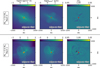 |
Fig. 1 Snapshots taken from the RAMSES MHD models (ℳ0 and ℳ1) of a collapsing protostellar envelope (initial parameters can be found in the text) with dust grain size evolution computed by COALA. The maps show a 2000 au zoom in on the model when the central star has accreted 0.4 M⊙from the initial 2.5 M⊙core. The red cross represents the position of the star. The left column shows the total column gas density, Σ. The middle column shows the average grain size at the peak of the size distribution, apeak, weighted by the gas density along the line of sight (see the main text for further details). Similarly, the right column shows the average dust enrichment (ratio between the evolved dust-to-gas ratio, ϵ, and the initial dust-to-gas ratio, ϵ0) weighted by the gas density along the line of sight. In the top row, the square patterns near the sink are not numerical artifacts but result from the weighted average of the quantities along the line of sight. |
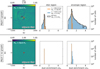 |
Fig. 2 Snapshots and histograms of the dust enrichment at two given times of model ℳ1 with (top row) and without (bottom row) dust growth. The histograms are obtained with the dust enrichment calculated in each cell in a box with sides of 2000 au around the star. The two times are when M⋆ = 0.06 M⊙ (orange) and M⋆ = 0.4 M⊙ (blue). Dust growth and dynamics result in larger local variations in the dust enrichment, by a factor of greater than 2, in the envelope compared to the dust dynamics alone. The black line shows the histograms for the ℳ1 model with dust growth and 60 dust bins, highlighting the numerical convergence reached with 40-bin simulations. The red cross represents the position of the star. The variance value of ~0.01 of the histogram explains the low variation observed on the map for model ℳ1 when M⋆ = 0.4 M⊙. |
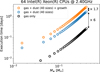 |
Fig. 3 Comparison of the computational times of the three simulations for model ℳ0: gas only (black), gas with 40 dust sizes (blue), and gas with 40 dust sizes and dust growth (orange). Using COALA in RAMSES only increases the global execution time by a factor of 1.7. |
4 Discussion
Figures 4a and 4c show the radial profiles of the dust grain size at the peak of the distribution, apeak, in the envelope (100 to 4000 au) for the two models (ℳ0 and ℳ1) at t0.4 M⊙. The radial profile was built by computing the mean apeak in concentric shells around the central star (see Appendix G). The mean value of apeak was calculated for the cells where the grain–grain differential velocity of grains with size apeak, noted δvapeak, is lower than the fragmentation velocity threshold. Both profiles show a clear increase in apeak, up to ~10 μm, with decreasing envelope radius. We used the fit function of the form f(x) ≡ a + bx−c. The power-law coefficient, c, goes from 0.9 for model ℳ0 to 1.1 for model ℳ1. This power law is perfectly consistent with the fact that the grain size is ![Mathematical equation: $\[\propto \sqrt{\rho}\]$](/articles/aa/full_html/2026/03/aa57277-25/aa57277-25-eq15.png) since the density scales roughly as
since the density scales roughly as ![Mathematical equation: $\[\propto \frac{1}{r^{2}}\]$](/articles/aa/full_html/2026/03/aa57277-25/aa57277-25-eq16.png) . We note that the slope is steeper in ℳ1 because turbulence (1) slows the collapse and (2) generates a dense filamentary structure far from the center. We observe that both models produce micron-sized grains, while model ℳ1 produces slightly larger grains (up to ~8 μm) in the envelope. We interpret this as being due to the turbulence slowing the collapse and generating dense regions away from the collapse center; this increases collision rates, which in turn favors dust growth.
. We note that the slope is steeper in ℳ1 because turbulence (1) slows the collapse and (2) generates a dense filamentary structure far from the center. We observe that both models produce micron-sized grains, while model ℳ1 produces slightly larger grains (up to ~8 μm) in the envelope. We interpret this as being due to the turbulence slowing the collapse and generating dense regions away from the collapse center; this increases collision rates, which in turn favors dust growth.
Figures 4b and 4d show 2D histograms of the grain size apeak according to the distance to the central star and δvapeak, the grain–grain differential velocity of grains with size apeak, from turbulence models (Ormel & Cuzzi 2007, see our Appendix A.1). In this model, the level of turbulence is reduced in the disk region (when nH > 109) in order to be consistent with the model of the α-viscosity disk (Birnstiel et al. 2010). Therefore, δvapeak is reduced by four orders of magnitude. The disk region is defined for low values of radii and δvapeak (cross marker). The point markers, located at higher values of δvapeak, define the envelope region. The accuracy of grain size predictions, when only considering dust growth, depends on the fragmentation limit used to evaluate if grains can survive. Our modeling does not yet include fragmentation processes, but as grains grow in size these processes are expected to become limiting factors to the dust growth. To mitigate the impact of this lacking physics, we used prescriptions from the literature to evaluate whether the grains formed in our models are expected to fragment. The hypotheses made to identify the parameter space where grains from our models are expected to fragment (blue and orange hashed regions in Figs. 4b and 4d) are as follows: To compute the fragmentation of the grains in our models, we first assumed grains are composed of 0.1 μm monomers. Second, we estimated the fragmentation velocity of the grains by comparing the kinetic energy of the grain and the energy required to break a bond between two monomers as vfrag ~ 22 m s−1 for silicates and vfrag ~ 300 m s−1 for ice-coated grains (Ormel et al. 2009; Lebreuilly et al. 2023b). Observations of Class 0 disks and hot-corino regions in low-mass protostars suggest that a significant fraction of the mass at r < 100 au is subject to accretion and viscous heating, with temperatures often higher than 50–100 K (Zamponi et al. 2021). Therefore, while dust grains are expected to be ice-coated in the envelope at radii r > 100 au, we assumed they are probably bare in the region r < 100 au. The fragmentation velocities for the two types of grains (ice-coated and bare grains) are respectively reported as orange and blue hashed areas in Figs. 4b and 4d. All grains with differential dust velocities (δvapeak; enhanced by gas turbulence from Ormel’s model; see our Appendix A.1) higher than these fragmentation velocities have a high probability of fragmenting and are thus ignored in the following discussion. Note that these differential velocities were computed by taking into account the collision between grains representing the bulk of the dust mass (e.g., with sizes close to apeak).
We stress that the fragmentation of dust grains in astrophysical environments is not well constrained, as the velocity threshold over which the grain-grain collision will result in grain fragmentation(s) depends on the microphysics properties of a grain, such as its size, shape, and composition. These grain properties are poorly constrained, and there is no consensus as to which grains survive which collisions. For instance, an analysis of grains collected by the Rosetta mission has shown that 50% of the aggregates with sizes of a few microns may have fragmented due to collecting velocities of ≳3–7 m s−1 (Kim et al. 2023). This velocity threshold is much lower than, for example, the theoretical value of 22 m s−1 widely used for bare silicate grains with the same porosity (Ormel et al. 2009). To better constrain the growth of grains up to sizes where their fragmentation is likely in protostellar envelopes, where typical gas velocities are a fraction of a kilometer per second, one needs to make a hypothesis regarding the structure of these grown grains, especially their porosity and fractal dimensions. Such a level of modeling is beyond the current state of the art: future COALA implementations will consistently treat both dust coagulation and fragmentation using a more realistic hypothesis.
To conclude, despite the fact that fragmentation processes are not yet included in the COALA dust evolution model implemented in RAMSES, most of the predicted grains with sizes of a few microns (1–10) are expected to survive in the envelope’s physical conditions. The grains ranging from 4.9 to 7.1 μm, which do not enter the fragmentation regime in the envelope, represent 0.5% of the total dust mass in model ℳ1, and 0.4% in model ℳ0. The precise evolution at disk scales requires a dedicated study that includes dust growth and fragmentation and discusses the hypothesis made regarding the disk model that results in the low values of δvapeak seen in Fig. 4. Interestingly, if grains grow easily to ~10 μm in the envelopes during the first stages of disk formation, before entering the disks and evolving further, this could explain some properties from the dust in comet 67P (Bentley et al. 2016). Indeed, dust particles collected by the Rosetta probe show that grains larger than 8 μm are more compact and less elongated than the smaller particles – as would be expected from compaction processes in a disk environment. However, micron-sized grains consist of porous agglomerates that are suggested to be hierarchical on a scale probably covering at least hundreds of nanometers to several micrometers, such as would be expected from the growth processes at work in envelope environments.
Figure 5 shows the evolution of the fraction of the total dust mass represented by each grain size bin in the envelope in model ℳ1. Grains can grow easily and very quickly to about 10 μm after 100 kyr in dense envelopes experiencing protostellar collapse. The mass fraction evolution of the grains with a size between ~3 and 5 μm reaches a steady state after 100 kyr, with a value of ~1% of the total dust mass.
The evolution of the dust size distribution affects the nonideal MHD resistivities and, thus, the magnetic braking and other magnetic effects (Zhao et al. 2016; Guillet et al. 2020; Silsbee et al. 2020; Kawasaki et al. 2022; Lebreuilly et al. 2023a). Resistivity evolution is governed by the evolution of the population of small grains. Because our model does not yet include fragmentation, the fraction of very small grains, which drives the ambilopar diffusion resistivity, is not accurately described in these current models. In a future study, we will include fragmentation to accurately account for the evolution of MHD resistivities.
Note that in this study, we did not consider the disruption of grains due to radiative torque from strong radiation fields (Hoang 2019; Reissl et al. 2024). This phenomenon may play an important role in the depletion of large grains in the envelope. This fragmentation process will be added in COALA to quantify which grains are rotationally disrupted to the extent that they affect the dust size distribution in the protostellar envelope, and the results will be compared with those of a previous study (Le Gouellec et al. 2023).
Our work shows that the dust size distribution rapidly evolves from the initial MRN distribution in protostellar envelopes due to the coagulation process, as shown in several previous studies (Bate 2022; Lebreuilly et al. 2023b; Vorobyov et al. 2025). Therefore, in disks whose material comes from the parent envelope, the initial dust size distribution most likely does not follow an MRN distribution and includes large, micron-sized dust grains. Such a different dust size distribution may significantly affect the disk evolution, as it will be key in several physical processes, such as the disk thermal equilibrium and the chemistry at the grain surfaces, that potentially modify the disk’s temperature, scale height, and structure. Moreover, a change in the pristine dust size distribution may also result in a different dust size evolution and spatial distribution in the young disks, as well as the coupling of the disk material with the local magnetic field.
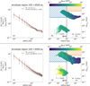 |
Fig. 4 Radial profiles of the dust grain size at the peak of the size distribution, apeak (see the main text for further details) and the grain-grain differential velocity of grains with size apeak from the turbulence models (see Appendix A.1), noted δvapeak, for the two snapshots shown in Fig. 1: models ℳ0 and ℳ1 at t0.4M⊙. Left panels: Radial profiles built by computing the mean apeak in concentric shells from the apeak map (for further details, see Fig. G.1 and the text). The mean dust grain size clearly increases with decreasing envelope radius, up to ~10 μm. The power law in model ℳ1 is higher than for model ℳ0. This shows that the grains grow faster in model ℳ1 since the gas turbulence tends to slow the collapse, leaving more time for grains to grow. Right panels: Dust grain populations (color-coded by apeak) at all envelope radii, plotted against the δvapeak they experience at this envelope location (in individual cells in the model). A vertical gray line represents the 100 au radius, approximating the ice line expected for such solar-type protostars. On each side of this line, orange and blue shaded areas represent the locations where the dust grains are expected to fragment (see text for further details). |
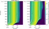 |
Fig. 5 Time evolution of the fraction of the total dust mass in the envelope represented by each grain size bin. Initially, the grains from 0.19 to 0.27 μm represent ~20% of the total dust mass. After 100 kyr, these grains account for ~13% of the total dust mass. A part of the mass is represented by larger grains, such as grains with sizes of ~3–5 μm, which represent a steady-state value of ~1% of the total dust mass (white lines). |
5 Conclusions
In this work we performed, for the first time, 3D nonideal MHD simulations of protostellar collapse that self-consistently account for dust dynamics and growth; we modeled the dust growth using the Smoluchowski equation and coupling the codes COALA and RAMSES. The new code COALA allowed us to include dust growth at a low numerical cost. This new numerical tool allowed us to run simulations beyond the current state of the art. Our goal was to predict the sizes of the grains expected to survive up until the fragmentation regime in a collapsing protostellar envelope during the disk formation stage. We ran two models, with and without an initial turbulent Mach, up to an evolutionary stage representative of a young embedded protostar. Our main findings are as follows:
In the envelope environment, dust grains grow rapidly to about 1–10 μm in both models (ℳ0 and ℳ1) and survive after 100 kyr from an initial MRN distribution;
In the disk region, the dust size distribution does not follow an MRN distribution and includes large grains of up to several tens of microns in size;
Dust growth results in a higher dust enrichment compared to dust dynamics alone. More models with various kernels are required to see how influential this can be on the dust content of the disk;
Dust evolution is highly anisotropic due to the nature of the collapse. There are preferred locations for the production of large grains, such as high-density structures from a turbulent infall (model ℳ1) or outflow cavity walls (model ℳ0).
Dust fragmentation processes from grain-grain collisions and radiative torque counterbalance dust growth and thus play key roles in shaping the dust size distribution. Therefore, it is essential to also self-consistently account for the dust fragmentation in 3D MHD simulations in order to precisely predict the local dust size distribution in the envelope and in the disk. An accurate prediction of the dust size distribution is key when studying several physical and chemical processes in the protostellar collapse. New 3D simulations of protostellar collapse with dust growth and fragmentation will be performed with the new tool {COALA + RAMSES} in a future study.
Acknowledgements
We thank the referee for providing very useful comments that helped us to improve our manuscript. This work was made possible thanks to the support from the European Research Council (ERC) under the European Union’s Horizon 2020 research and innovation program (Grant agreement No. 101098309 – PEBBLES). The simulations were carried out on the Alfven supercomputing cluster of the Commissariat à l’Énergie Atomique et aux énergies alternatives (CEA). Post-processing and data visualization was done using the open source Osyris package.
References
- Bate, M. R. 2022, MNRAS, 514, 2145 [CrossRef] [Google Scholar]
- Bate, M. R., Hutchison, M. A., & Elsender, D. 2025, arXiv e-prints [arXiv:2512.06409] [Google Scholar]
- Bentley, M. S., Schmied, R., Mannel, T., et al. 2016, Nature, 537, 73 [Google Scholar]
- Birnstiel, T. 2024, ARA&A, 62, 157 [NASA ADS] [CrossRef] [Google Scholar]
- Birnstiel, T., Dullemond, C. P., & Brauer, F. 2010, A&A, 513, A79 [NASA ADS] [CrossRef] [EDP Sciences] [Google Scholar]
- Bracco, A., Palmeirim, P., André, P., et al. 2017, A&A, 604, A52 [NASA ADS] [CrossRef] [EDP Sciences] [Google Scholar]
- Cacciapuoti, L., Macias, E., Maury, A. J., et al. 2023, A&A, 676, A4 [NASA ADS] [CrossRef] [EDP Sciences] [Google Scholar]
- Dartois, E., Noble, J. A., Caselli, P., et al. 2024, Nat. Astron., 8, 359 [NASA ADS] [CrossRef] [Google Scholar]
- Draine, B. T. 2003, ARA&A, 41, 241 [NASA ADS] [CrossRef] [Google Scholar]
- Drążkowska, J., Li, S., Birnstiel, T., Stammler, S. M., & Li, H. 2019, ApJ, 885, 91 [Google Scholar]
- Elbakyan, V. G., Johansen, A., Lambrechts, M., Akimkin, V., & Vorobyov, E. I. 2020, A&A, 637, A5 [NASA ADS] [CrossRef] [EDP Sciences] [Google Scholar]
- Epstein, P. S. 1924, Phys. Rev., 23, 710 [Google Scholar]
- Galametz, M., Maury, A. J., Valdivia, V., et al. 2019, A&A, 632, A5 [NASA ADS] [CrossRef] [EDP Sciences] [Google Scholar]
- Gong, M., Ivlev, A. V., Zhao, B., & Caselli, P. 2020, ApJ, 891, 172 [NASA ADS] [CrossRef] [Google Scholar]
- Gong, M., Ivlev, A. V., Akimkin, V., & Caselli, P. 2021, ApJ, 917, 82 [NASA ADS] [CrossRef] [Google Scholar]
- Gottlieb, S., Ketcheson, D. I., & Shu, C.-W. 2009, J. Sci. Comput., 38, 38 [Google Scholar]
- Guillet, V., Hennebelle, P., Pineau des Forêts, G., et al. 2020, A&A, 643, A17 [EDP Sciences] [Google Scholar]
- Ho, K. W., Li, H., & Li, S. 2024, ApJ, 975, L34 [Google Scholar]
- Hoang, T. 2019, ApJ, 876, 13 [NASA ADS] [CrossRef] [Google Scholar]
- Kawasaki, Y., Koga, S., & Machida, M. N. 2022, MNRAS, 515, 2072 [NASA ADS] [CrossRef] [Google Scholar]
- Kim, M., Mannel, T., Boakes, P. D., et al. 2023, A&A, 673, A129 [NASA ADS] [CrossRef] [EDP Sciences] [Google Scholar]
- Kwon, W., Looney, L. W., Mundy, L. G., Chiang, H.-F., & Kemball, A. J. 2009, ApJ, 696, 841 [NASA ADS] [CrossRef] [Google Scholar]
- Le Gouellec, V. J. M., Maury, A. J., Hull, C. L. H., et al. 2023, A&A, 675, A133 [NASA ADS] [CrossRef] [EDP Sciences] [Google Scholar]
- Lebreuilly, U., Commerçon, B., & Laibe, G. 2019, A&A, 626, A96 [NASA ADS] [CrossRef] [EDP Sciences] [Google Scholar]
- Lebreuilly, U., Commerçon, B., & Laibe, G. 2020, A&A, 641, A112 [EDP Sciences] [Google Scholar]
- Lebreuilly, U., Mac Low, M. M., Commerçon, B., & Ebel, D. S. 2023a, A&A, 675, A38 [NASA ADS] [CrossRef] [EDP Sciences] [Google Scholar]
- Lebreuilly, U., Vallucci-Goy, V., Guillet, V., Lombart, M., & Marchand, P. 2023b, MNRAS, 518, 3326 [Google Scholar]
- Li, Y.-P., Li, H., Li, S., et al. 2020, ApJ, 892, L19 [NASA ADS] [CrossRef] [Google Scholar]
- Lombart, M., & Laibe, G. 2021, MNRAS, 501, 4298 [Google Scholar]
- Marchand, P., Guillet, V., Lebreuilly, U., & Mac Low, M. M. 2021, A&A, 649, A50 [NASA ADS] [CrossRef] [EDP Sciences] [Google Scholar]
- Marchand, P., Lebreuilly, U., Mac Low, M. M., & Guillet, V. 2023, A&A, 670, A61 [NASA ADS] [CrossRef] [EDP Sciences] [Google Scholar]
- Masson, J., Teyssier, R., Mulet-Marquis, C., Hennebelle, P., & Chabrier, G. 2012, ApJS, 201, 24 [Google Scholar]
- Mathis, J. S., Rumpl, W., & Nordsieck, K. H. 1977, ApJ, 217, 425 [Google Scholar]
- Maury, A. J., André, P., Testi, L., et al. 2019, A&A, 621, A76 [NASA ADS] [CrossRef] [EDP Sciences] [Google Scholar]
- Miotello, A., Testi, L., Lodato, G., et al. 2014, A&A, 567, A32 [NASA ADS] [CrossRef] [EDP Sciences] [Google Scholar]
- Ormel, C. W., & Cuzzi, J. N. 2007, A&A, 466, 413 [NASA ADS] [CrossRef] [EDP Sciences] [Google Scholar]
- Ormel, C. W., Paszun, D., Dominik, C., & Tielens, A. G. G. M. 2009, A&A, 502, 845 [NASA ADS] [CrossRef] [EDP Sciences] [Google Scholar]
- Pfeil, T., Birnstiel, T., & Klahr, H. 2024, A&A, 691, A45 [NASA ADS] [CrossRef] [EDP Sciences] [Google Scholar]
- Reissl, S., Nguyen, P., Jordan, L. M., & Klessen, R. S. 2024, A&A, 692, A60 [NASA ADS] [CrossRef] [EDP Sciences] [Google Scholar]
- Robinson, A., Booth, R. A., & Owen, J. E. 2024, MNRAS, 529, 1524 [Google Scholar]
- Silsbee, K., Ivlev, A. V., Sipilä, O., Caselli, P., & Zhao, B. 2020, A&A, 641, A39 [NASA ADS] [CrossRef] [EDP Sciences] [Google Scholar]
- Stammler, S. M., & Birnstiel, T. 2022, ApJ, 935, 35 [NASA ADS] [CrossRef] [Google Scholar]
- Stepinski, T. F., & Valageas, P. 1996, A&A, 309, 301 [NASA ADS] [Google Scholar]
- Tanaka, H., Inaba, S., & Nakazawa, K. 1996, Icarus, 123, 450 [Google Scholar]
- Testi, L., Birnstiel, T., Ricci, L., et al. 2014, in Protostars and Planets VI, eds. H. Beuther, R. S. Klessen, C. P. Dullemond, & T. Henning, 339 [Google Scholar]
- Teyssier, R. 2002, A&A, 385, 337 [CrossRef] [EDP Sciences] [Google Scholar]
- Truelove, J. K., Klein, R. I., McKee, C. F., et al. 1997, ApJ, 489, L179 [CrossRef] [Google Scholar]
- Tsukamoto, Y., Machida, M. N., & Inutsuka, S.-i. 2021, ApJ, 920, L35 [NASA ADS] [CrossRef] [Google Scholar]
- Valdivia, V., Maury, A., & Hennebelle, P. 2022, A&A, 668, A83 [NASA ADS] [CrossRef] [EDP Sciences] [Google Scholar]
- Vallucci-Goy, V., Lebreuilly, U., & Hennebelle, P. 2024, A&A, 690, A23 [NASA ADS] [CrossRef] [EDP Sciences] [Google Scholar]
- Vorobyov, E. I., & Elbakyan, V. G. 2019, A&A, 631, A1 [NASA ADS] [CrossRef] [EDP Sciences] [Google Scholar]
- Vorobyov, E. I., Kulikov, I., Elbakyan, V. G., McKevitt, J., & Güdel, M. 2024, A&A, 683, A202 [NASA ADS] [CrossRef] [EDP Sciences] [Google Scholar]
- Vorobyov, E. I., Elbakyan, V. G., Skliarevskii, A., Akimkin, V., & Kulikov, I. 2025, A&A, 699, A27 [NASA ADS] [CrossRef] [EDP Sciences] [Google Scholar]
- Ysard, N., Abergel, A., Ristorcelli, I., et al. 2013, A&A, 559, A133 [NASA ADS] [CrossRef] [EDP Sciences] [Google Scholar]
- Zamponi, J., Maureira, M. J., Zhao, B., et al. 2021, MNRAS, 508, 2583 [NASA ADS] [CrossRef] [Google Scholar]
- Zhao, B., Caselli, P., Li, Z.-Y., et al. 2016, MNRAS, 460, 2050 [Google Scholar]
Appendix A Grain-grain differential velocities
In this study, the sources of the grain-grain differential velocities are the turbulence, the Brownian motion and the hydrodynamical drift.
Appendix A.1 Differential velocity from gas turbulence
The gas turbulence is a source of relative velocity between grains through the drag force. The strength of this turbulent motion depends on the grain size and the Reynolds number Re. Ormel & Cuzzi (2007) formulated the expression of the relative velocity between two grains i (the larger grain) and j (the smaller grain) in three regimes which depends on the Stokes number Sti ≡ ts,i/tdyn where tdyn is the dynamical timescale of the system. As shown in Marchand et al. (2021), we can consider only the intermediate regime in the context of the collapse. In that case, the differential velocity writes
![Mathematical equation: $\[\Delta v_{\text {turb}, i, j} \equiv \sqrt{\alpha \beta_{i, j}} c_{\mathrm{s}} ~\sqrt{\mathrm{St}_i},\]$](/articles/aa/full_html/2026/03/aa57277-25/aa57277-25-eq17.png) (A.1)
(A.1)
The term βi,j is written as
![Mathematical equation: $\[\beta_{i, j}=3.2-\left(1+\xi_{i, j}\right)+\frac{2}{1+\xi_{i, j}}\left(\frac{1}{2.6}+\frac{\xi_{i, j}^3}{1.6+\xi_{i, j}}\right),\]$](/articles/aa/full_html/2026/03/aa57277-25/aa57277-25-eq18.png) (A.2)
(A.2)
where ξi,j ≡ Sti/Stj. In this study, the α coefficient, describing the level of turbulence, has a value of 1.5 in the envelope and 10−4 in the disk region, defined with a criteria on the number density of hydrogen nH > 109 cm−3. As in Tsukamoto et al. (2021), we compute the dynamical time as
![Mathematical equation: $\[t_{\mathrm{dyn}}=\frac{c_{\mathrm{s}}}{\left|\boldsymbol{a}_{\mathrm{g}}\right|},\]$](/articles/aa/full_html/2026/03/aa57277-25/aa57277-25-eq19.png) (A.3)
(A.3)
ag being the gravitational acceleration.
Appendix A.2 Brownian motion
The differential velocity between two grains of masses mi and mj is formulated as
![Mathematical equation: $\[\Delta v_{\mathrm{Br}, i, j} \equiv \sqrt{\frac{8 k_{\mathrm{B}} T}{\pi}} \sqrt{\frac{1}{m_i}+\frac{1}{m_j}},\]$](/articles/aa/full_html/2026/03/aa57277-25/aa57277-25-eq20.png) (A.4)
(A.4)
where kb is the Boltzmann constant and T the gas temperature. The differential velocity increases as the masses of the grains decrease. Therefore, the dust growth by Brownian motion is efficient for small grains.
Appendix A.3 Hydrodynamical drift
The dynamics of the grains depends on their size due to the drag force from the gas. Therefore, two grains of different sizes can collide. The relative velocity between grains sizes i and j is written as
![Mathematical equation: $\[\Delta v_{\mathrm{drift}, i, j} \equiv\left|\boldsymbol{v}_i-\boldsymbol{v}_j\right|.\]$](/articles/aa/full_html/2026/03/aa57277-25/aa57277-25-eq21.png) (A.5)
(A.5)
This velocity is named hydrodynamical drift velocity.
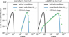 |
Fig. B.1 Benchmarks of the code COALA to solve the Smoluchowski coagulation equation (Eq. (1)) with the constant and the additive kernels. In the two plots, the y-axis are the dust grain mass distribution and the x-axis the grain masses in dimensionless unit. The mass range is chosen in order to have 19 orders of magnitude in mass similar to the mass range obtained from smin = 5 nm to smax = 1 nm. The black lines are the initial mass distribution. The blue lines are the exact solutions at a final time tfinal. The green circle are the numerical solutions for which the mass range is sampled in 40 mass bins. The numerical solutions follow accurately the exact solutions. |
Appendix B Benchmarking COALA
The code COALA is benchmarked with solutions to the Smoluchowski equation, for the constant and additive kernel, in order to check the good accuracy in the setup with the coupling to the code RAMSES. The mass range spans 19 orders of magnitude, which is similar to the one obtained from the size range smin = 5 nm to smax = 1 nm. The mass range is discretized in 40 bins. The results are shown in Fig. B.1 where the numerical solutions are in green and the exact ones are in blue. In both tests, the analytical solution is well reproduced up to a final time where grains grown by 3 orders of magnitude in size. We note a slight numerical diffusion at the high mass tail for the additive kernel. This numerical problem is well known from most of the solvers for the Smoluchowski equation. The new code COALA is well designed to drastically reduce this numerical diffusion by taking advantage of high-order approximation (Lombart & Laibe 2021). In this study, only the piecewise constant approximation is used to keep low numerical costs for the 3D simulations.
Appendix C Selected region in the simulation for the analysis
The RAMSES simulations is around 32000 au side. As indicated in 3, we select 8000 au side cube in order to exclude the impact of the grid boundaries. Figure C.1 shows the full map and the selected region in the edge-on view.
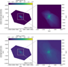 |
Fig. C.1 Selected cube of 8000 au sides (grey square) in the simulations of around 32000 au side to perform the analysis in Fig. 4. Upper row: Total column gas density maps. Lower row: Grain size at the peak of the dust size distribution. |
Appendix D Line-of-sight averaged quantities
The two average quantities shown in the maps and discussed throughout the paper are calculated as
![Mathematical equation: $\[a_{\mathrm{peak}} \equiv a_{\mathrm{peak}, i, j}=\frac{\sum_k a_{\mathrm{peak}, i, j, k} ~\rho_{i, j, k}}{\sum_k \rho_{i, j, k}}, \frac{\epsilon}{\epsilon_0} \equiv \frac{\epsilon_{i, j}}{\epsilon_0}=\frac{\sum_k \frac{\epsilon_{i, j, k}}{\epsilon_0} \rho_{i, j, k}}{\sum_k \rho_{i, j, k}},\]$](/articles/aa/full_html/2026/03/aa57277-25/aa57277-25-eq22.png) (D.1)
(D.1)
where i, j and k are the indices for the spatial coordinates of the cells, for which k is the index of the direction along the line of sight. The quantities apeak,i,j,k and ϵi,j,k are the grain size at the peak of the size distribution and the dust-to-gas ratio in a given cell.
Appendix E Scaling of the peak of the dust size distribution
We demonstrate here a simple relation between the typical grain size s and the gas density ρ. We assume a simple spherical collapse such as
![Mathematical equation: $\[\frac{d \rho}{d t}=\frac{\rho}{t_{\mathrm{ff}}},\]$](/articles/aa/full_html/2026/03/aa57277-25/aa57277-25-eq23.png) (E.1)
(E.1)
and a monodisperse formulation of the grain size evolution (Stepinski & Valageas 1996; Tsukamoto et al. 2021)
![Mathematical equation: $\[\frac{d s}{d t}=\frac{s}{3 t_{\mathrm{coag}}},\]$](/articles/aa/full_html/2026/03/aa57277-25/aa57277-25-eq24.png) (E.2)
(E.2)
where the coagulation timescale writes
![Mathematical equation: $\[t_{\mathrm{coag}}=\frac{m_d}{4 \pi s^2 \rho_d \Delta v},\]$](/articles/aa/full_html/2026/03/aa57277-25/aa57277-25-eq25.png) (E.3)
(E.3)
and the free-fall timescale writes
![Mathematical equation: $\[t_{\mathrm{ff}}=\sqrt{\frac{3 \pi}{32 G \rho}}.\]$](/articles/aa/full_html/2026/03/aa57277-25/aa57277-25-eq26.png) (E.4)
(E.4)
Combining the two equations yields
![Mathematical equation: $\[\frac{d s}{d \rho}=\frac{s}{3 \rho} \frac{t_{\mathrm{ff}}}{t_{\mathrm{coag}}}.\]$](/articles/aa/full_html/2026/03/aa57277-25/aa57277-25-eq27.png) (E.5)
(E.5)
Assuming coagulation by turbulence, we can write
![Mathematical equation: $\[\Delta v=A \sqrt{\frac{t_{\mathrm{s}}}{t_{\mathrm{ff}}}}.\]$](/articles/aa/full_html/2026/03/aa57277-25/aa57277-25-eq28.png) (E.6)
(E.6)
Finally, injecting Eq. 4 with Sgrain ← s and Eqs. E.3, E.4, and E.6 into Eq. E.5, we obtain
![Mathematical equation: $\[\frac{d s}{\sqrt{s}}=\left(\frac{3 \pi}{32 G}\right)^{1 / 4} A \frac{\epsilon_{\mathrm{dg}}}{\sqrt{\rho_{\mathrm{grain}}}} \frac{1}{\sqrt{w_{\mathrm{th}}}} \frac{d \rho}{\rho^{3 / 4}},\]$](/articles/aa/full_html/2026/03/aa57277-25/aa57277-25-eq29.png) (E.7)
(E.7)
where ϵdg ≡ ρdust/ρ is the dust-to-gas ratio. By integration we finally get
![Mathematical equation: $\[\sqrt{s(t)}-\sqrt{s_0}=2\left(\frac{3 \pi}{32 G}\right)^{1 / 4} A \frac{\epsilon_{\mathrm{dg}}}{\sqrt{\rho_{\mathrm{grain}}}} \frac{1}{\sqrt{w_{\mathrm{th}}}}\left[\rho(t)^{1 / 4}-\rho_0^{1 / 4}\right],\]$](/articles/aa/full_html/2026/03/aa57277-25/aa57277-25-eq30.png) (E.8)
(E.8)
or
![Mathematical equation: $\[s(t)=\left(2\left(\frac{3 \pi}{32 G}\right)^{1 / 4} A \frac{\epsilon_{\mathrm{dg}}}{\sqrt{\rho_{\text {grain }}}} \frac{1}{\sqrt{w_{\text {th }}}}\left[\rho(t)^{1 / 4}-\rho_0^{1 / 4}\right]+\sqrt{s_0}\right)^2.\]$](/articles/aa/full_html/2026/03/aa57277-25/aa57277-25-eq31.png) (E.9)
(E.9)
Assuming a small initial size and density yields
![Mathematical equation: $\[s(t)=4\left(\frac{3 \pi}{32 G}\right)^{1 / 2} A^2 \frac{\epsilon_{\mathrm{dg}}^2}{\rho_{\text {grain }}} \frac{1}{w_{\mathrm{th}}} \sqrt{\rho}.\]$](/articles/aa/full_html/2026/03/aa57277-25/aa57277-25-eq32.png) (E.10)
(E.10)
We note that ![Mathematical equation: $\[A \simeq \sqrt{2 \alpha} c_{s}\]$](/articles/aa/full_html/2026/03/aa57277-25/aa57277-25-eq33.png) and
and ![Mathematical equation: $\[w_{\text {th}}=\sqrt{\frac{8}{\pi \gamma}} c_{s}\]$](/articles/aa/full_html/2026/03/aa57277-25/aa57277-25-eq34.png) . We finally get
. We finally get
![Mathematical equation: $\[s(t) \simeq \sqrt{8 \pi \gamma}\left(\frac{3 \pi}{32 G}\right)^{1 / 2} \alpha c_s \frac{\epsilon_{\mathrm{dg}}^2}{\rho_{\text {grain }}} \sqrt{\rho}\]$](/articles/aa/full_html/2026/03/aa57277-25/aa57277-25-eq35.png) (E.11)
(E.11)
Or
![Mathematical equation: $\[\begin{aligned}s(t) \simeq~ & 0.004 \mathrm{~cm}\left(\frac{\alpha}{1}\right)\left(\frac{T}{10 K}\right)^{1 / 2}\left(\frac{\epsilon_{\mathrm{dg}}}{0.01}\right)^2\left(\frac{\rho_{\text {grain }}}{2.3 \mathrm{~g} \mathrm{~cm}^{-3}}\right)^{-1} \\& \left(\frac{\rho}{10^{-13} \mathrm{~g} \mathrm{~cm}^{-3}}\right)\end{aligned}\]$](/articles/aa/full_html/2026/03/aa57277-25/aa57277-25-eq36.png) (E.12)
(E.12)
We point out that, as shown in Lebreuilly et al. (2020), the Stokes number St, which is the ratio between the stopping time and the free-fall time scales as ![Mathematical equation: $\[\propto \frac{s}{\sqrt{\rho}}\]$](/articles/aa/full_html/2026/03/aa57277-25/aa57277-25-eq37.png) . This means that this quantity is roughly constant in the isothermal regions of the collapse when dust growth is included.
. This means that this quantity is roughly constant in the isothermal regions of the collapse when dust growth is included.
Appendix F Model ℳ1 with and without dust growth
In Fig. F.1 we compare simulations of the model ℳ1 with (bottom row) and without (top row) dust growth. The total column density Σ and apeakare defined in Sect. 3. The dust growth highlights the anisotropy of the dust evolution, where grains grow faster in some specific regions, i.e. structures due to turbulent infall in the model ℳ1. We note that the initial MRN distribution evolved locally in the simulation due to the dust growth.
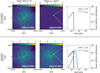 |
Fig. F.1 Comparison without dust growth (upper row) and with dust growth (lower row) for the model ℳ1 with M⋆ = 0.4M⊙. The red cross gives the position of the star. The left and middle columns show the total column gas density Σ and the average grain size at the peak of the dust size distribution apeak similarly to Fig. 1. For the model without growth, the apeak is the maximum size of the MRN distribution (~250 nm). The right column shows the evolution of the dust size distribution in a cell in the simulation. |
Appendix G Radial profile of the dust size distribution
The radial profile of the dust size distribution in the 3D simulation is built by computing the mean of the dust size distribution in selected concentric shells around the star. The width of the shells is defined as 10% of the radius in order to capture enough cells to compute the mean. Figure G.1 shows the shells with radius [100,200,300,400,500] (top row) with the corresponding average dust size distribution (bottom row). From these average dust size distributions, we compute the mean grain size apeak at the peak of the distribution.
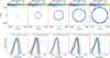 |
Fig. G.1 Radial dependence of the dust grain size distribution, from the model ℳ1 with M⋆ = 0.4 M⊙. Concentric shells of varying radii from 100 to 4000 au (as shown in the upper panels) are used to compute the mean dust grain size distributions shown in the lower panels. The dust grains size distribution is represented by the mass fraction distribution (see text for details). Here only the five first concentric shells with radius [100,200,300,400,500] au are shown in upper panel with the corresponding average dust grain size distribution weighted by the gas density (blue line) in the lower panel. The dust grain size distributions in each cell defining the shell are shown (light grey lines) in the lower panel. |
Single or two grain sizes, potentially varying locally.
This corresponds to a thermal-to-gravitational energy ratio of α = 0.35.
All Figures
|
Fig. 1 Snapshots taken from the RAMSES MHD models (ℳ0 and ℳ1) of a collapsing protostellar envelope (initial parameters can be found in the text) with dust grain size evolution computed by COALA. The maps show a 2000 au zoom in on the model when the central star has accreted 0.4 M⊙from the initial 2.5 M⊙core. The red cross represents the position of the star. The left column shows the total column gas density, Σ. The middle column shows the average grain size at the peak of the size distribution, apeak, weighted by the gas density along the line of sight (see the main text for further details). Similarly, the right column shows the average dust enrichment (ratio between the evolved dust-to-gas ratio, ϵ, and the initial dust-to-gas ratio, ϵ0) weighted by the gas density along the line of sight. In the top row, the square patterns near the sink are not numerical artifacts but result from the weighted average of the quantities along the line of sight. |
| In the text | |
|
Fig. 2 Snapshots and histograms of the dust enrichment at two given times of model ℳ1 with (top row) and without (bottom row) dust growth. The histograms are obtained with the dust enrichment calculated in each cell in a box with sides of 2000 au around the star. The two times are when M⋆ = 0.06 M⊙ (orange) and M⋆ = 0.4 M⊙ (blue). Dust growth and dynamics result in larger local variations in the dust enrichment, by a factor of greater than 2, in the envelope compared to the dust dynamics alone. The black line shows the histograms for the ℳ1 model with dust growth and 60 dust bins, highlighting the numerical convergence reached with 40-bin simulations. The red cross represents the position of the star. The variance value of ~0.01 of the histogram explains the low variation observed on the map for model ℳ1 when M⋆ = 0.4 M⊙. |
| In the text | |
|
Fig. 3 Comparison of the computational times of the three simulations for model ℳ0: gas only (black), gas with 40 dust sizes (blue), and gas with 40 dust sizes and dust growth (orange). Using COALA in RAMSES only increases the global execution time by a factor of 1.7. |
| In the text | |
|
Fig. 4 Radial profiles of the dust grain size at the peak of the size distribution, apeak (see the main text for further details) and the grain-grain differential velocity of grains with size apeak from the turbulence models (see Appendix A.1), noted δvapeak, for the two snapshots shown in Fig. 1: models ℳ0 and ℳ1 at t0.4M⊙. Left panels: Radial profiles built by computing the mean apeak in concentric shells from the apeak map (for further details, see Fig. G.1 and the text). The mean dust grain size clearly increases with decreasing envelope radius, up to ~10 μm. The power law in model ℳ1 is higher than for model ℳ0. This shows that the grains grow faster in model ℳ1 since the gas turbulence tends to slow the collapse, leaving more time for grains to grow. Right panels: Dust grain populations (color-coded by apeak) at all envelope radii, plotted against the δvapeak they experience at this envelope location (in individual cells in the model). A vertical gray line represents the 100 au radius, approximating the ice line expected for such solar-type protostars. On each side of this line, orange and blue shaded areas represent the locations where the dust grains are expected to fragment (see text for further details). |
| In the text | |
|
Fig. 5 Time evolution of the fraction of the total dust mass in the envelope represented by each grain size bin. Initially, the grains from 0.19 to 0.27 μm represent ~20% of the total dust mass. After 100 kyr, these grains account for ~13% of the total dust mass. A part of the mass is represented by larger grains, such as grains with sizes of ~3–5 μm, which represent a steady-state value of ~1% of the total dust mass (white lines). |
| In the text | |
|
Fig. B.1 Benchmarks of the code COALA to solve the Smoluchowski coagulation equation (Eq. (1)) with the constant and the additive kernels. In the two plots, the y-axis are the dust grain mass distribution and the x-axis the grain masses in dimensionless unit. The mass range is chosen in order to have 19 orders of magnitude in mass similar to the mass range obtained from smin = 5 nm to smax = 1 nm. The black lines are the initial mass distribution. The blue lines are the exact solutions at a final time tfinal. The green circle are the numerical solutions for which the mass range is sampled in 40 mass bins. The numerical solutions follow accurately the exact solutions. |
| In the text | |
|
Fig. C.1 Selected cube of 8000 au sides (grey square) in the simulations of around 32000 au side to perform the analysis in Fig. 4. Upper row: Total column gas density maps. Lower row: Grain size at the peak of the dust size distribution. |
| In the text | |
|
Fig. F.1 Comparison without dust growth (upper row) and with dust growth (lower row) for the model ℳ1 with M⋆ = 0.4M⊙. The red cross gives the position of the star. The left and middle columns show the total column gas density Σ and the average grain size at the peak of the dust size distribution apeak similarly to Fig. 1. For the model without growth, the apeak is the maximum size of the MRN distribution (~250 nm). The right column shows the evolution of the dust size distribution in a cell in the simulation. |
| In the text | |
|
Fig. G.1 Radial dependence of the dust grain size distribution, from the model ℳ1 with M⋆ = 0.4 M⊙. Concentric shells of varying radii from 100 to 4000 au (as shown in the upper panels) are used to compute the mean dust grain size distributions shown in the lower panels. The dust grains size distribution is represented by the mass fraction distribution (see text for details). Here only the five first concentric shells with radius [100,200,300,400,500] au are shown in upper panel with the corresponding average dust grain size distribution weighted by the gas density (blue line) in the lower panel. The dust grain size distributions in each cell defining the shell are shown (light grey lines) in the lower panel. |
| In the text | |
Current usage metrics show cumulative count of Article Views (full-text article views including HTML views, PDF and ePub downloads, according to the available data) and Abstracts Views on Vision4Press platform.
Data correspond to usage on the plateform after 2015. The current usage metrics is available 48-96 hours after online publication and is updated daily on week days.
Initial download of the metrics may take a while.