| Issue |
A&A
Volume 707, March 2026
|
|
|---|---|---|
| Article Number | A5 | |
| Number of page(s) | 18 | |
| Section | Extragalactic astronomy | |
| DOI | https://doi.org/10.1051/0004-6361/202557448 | |
| Published online | 25 February 2026 | |
Probing the star formation main sequence down to 107 M⊙ at 1 < z < 9
1
Institute for Computational Astrophysics and Department of Astronomy and Physics, Saint Mary’s University 923 Robie Street Halifax NS B3H 3C3, Canada
2
Columbia Astrophysics Laboratory, Columbia University 550 West 120th Street New York NY 10027, USA
3
Space Telescope Science Institute 3700 San Martin Drive Baltimore Maryland 21218, USA
4
National Research Council of Canada, Herzberg Astronomy & Astrophysics Research Centre 5071 West Saanich Road Victoria BC V9E 2E7, Canada
5
Faculty of Mathematics and Physics Jadranska ulica 19 SI-1000 Ljubljana, Slovenia
6
Department of Physics and Astronomy, University of California Davis 1 Shields Avenue Davis CA 95616, USA
7
Kapteyn Astronomical Institute, University of Groningen P.O. Box 800 9700AV Groningen, The Netherlands
8
Department of Physics and Astronomy, York University 4700 Keele St. Toronto Ontario M3J 1P3, Canada
9
Observatorio Astronómico de Córdoba, Universidad Nacional de Córdoba Laprida 854 X5000 Córdoba, Argentina
★ Corresponding author: This email address is being protected from spambots. You need JavaScript enabled to view it.
Received:
26
September
2025
Accepted:
12
January
2026
Abstract
The main sequence of star-forming galaxies (SFGMS or MS) is a fundamental scaling relation that provides a global framework for studying galaxy formation and evolution, as well as an insight into the complex star formation histories (SFHs) of individual galaxies. In this work, we combine large-area pre-JWST surveys (COSMOS2020, CANDELS), which probe high-M★ sources (> 109 M⊙), with SHARDS/CANDELS FAINT and JWST data from CANUCS, CEERS, JADES, and UNCOVER, to obtain a high-z, star formation rate (SFR) and stellar mass (M★) complete sample spanning both high- and low-M★ regimes. Completeness in both M★ and the SFR is key to avoiding biases introduced by low-mass, highly star-forming objects. Our combined dataset is 80% complete down to 107.6 M⊙ at z ∼ 1 (108.8 M⊙ at z ∼ 9). The overall intrinsic MS slope (based on the SFR100 and M★ derived with Dense Basis and nonparametric SFHs) shows little evolution up to z ∼ 5, with values ∼0.7 − 0.8. The slope in the low-M★ regime becomes steeper than that in the high-M★ end at least up to z ∼ 5, but the strength of this change is highly dependent on the assumptions made on the symmetry of the uncertainties in M★ and SFR. If real, the steepening suggests reduced star formation efficiency or declining gas content with decreasing M★. The transition between the low-M★ regime and the canonical MS occurs around 109.5 M⊙, independent of z. This critical value may coincide with the assembly of galaxies’ disks, which can provide a mechanism for self-regulation that stabilizes them against feedback. The intrinsic scatter is compatible with canonical estimates, also at low-M★, ranging from 0.2 − 0.3 dex. This is indicative of rapid variations in star formation being averaged out over ≲100 Myr.
Key words: galaxies: evolution / galaxies: high-redshift / galaxies: photometry / galaxies: star formation
© The Authors 2026
 Open Access article, published by EDP Sciences, under the terms of the Creative Commons Attribution License (https://creativecommons.org/licenses/by/4.0), which permits unrestricted use, distribution, and reproduction in any medium, provided the original work is properly cited.
This article is published in open access under the Subscribe to Open model. This email address is being protected from spambots. You need JavaScript enabled to view it. to support open access publication.
1. Introduction
Scaling relations manifest the combined action of the diverse and complex physical processes undergone by galaxies. They serve as benchmarks for any theoretical model exploring galaxy formation and evolution. These relations allow us to look past the plethora of local-scale phenomena, predict future evolutionary phases, and provide a cohesive global picture built from direct observables (e.g., the Schmidt-Kennicutt law of star formation; Schmidt 1959; Kennicutt 1989).
Despite the power of these tools, the overall picture of the formation and evolution of galaxies is still incomplete. Before the arrival of JWST, observing the faint Universe at high z was a challenging goal. Our understanding of the early epochs was based on observations of bright objects (Malmquist bias; Malmquist 1922). However, these bright sources may not exhibit or be primarily governed by the same processes that dominate fainter galaxies. Some of these faint objects correspond to massive systems whose emission remains undetected in the rest-frame optical, with more prominent spectral energy distributions (SEDs) at longer wavelengths (e.g., star-forming galaxies, SFGs, with high dust content; see Alcalde Pampliega et al. 2019; Zhou et al. 2020). However, a vast number of objects that lie beyond the sensitivities of pre-JWST optical and near-infrared (NIR) capabilities are actually low-mass galaxies (e.g., Austin et al. 2023; Mérida et al. 2023, M+23 hereafter; Strait et al. 2023; Asada et al. 2023, 2024; Looser et al. 2024b).
The mass-completeness limits achieved thanks to the Hubble Space Telescope (HST) sensitivity allowed us to reach down to 108.6 M⊙ at z = 1 (1010 M⊙ at z = 8) (Barro et al. 2019, B+19 hereafter). Some strategies that enabled the recovery of lower-luminosity (lower-mass) galaxies at high-z in the HST era involved exploiting gravitational lensing (e.g., Caputi et al. 2021; Sun et al. 2021); absorption systems (e.g., Lofthouse et al. 2020; Joshi et al. 2025); emission lines (e.g., Maseda et al. 2014; Atek et al. 2022); or stacking techniques (e.g., M+23, Mérida et al. 2024; Wang et al. 2024). Nowadays, these limits are easy to push thanks to the depth and sensitivity of new-generation telescopes.
However, even if we can detect these low-mass systems, it is important to note that the calibrations and conversions used to compute integrated quantities were derived from the low-z picture. Looking for analogs of low-z low-mass galaxies, such as extremely metal-poor galaxies, blue compact dwarfs, or damped Lyman-α systems (e.g., Wolfe et al. 2005; Cairós et al. 2010; Lorenzo et al. 2022), was key. Now, we can start studying the interstellar medium (ISM) of low-mass high-z galaxies themselves (e.g., Lin et al. 2023; Harshan et al. 2024; Looser et al. 2024a; D’Eugenio et al. 2025), which provides the means to improve calibrations.
A powerful scaling relation that was often extrapolated to lower stellar masses (M★) is the so-called main sequence of star-forming galaxies (SFGMS or MS; e.g., Daddi et al. 2007; Noeske et al. 2007; Elbaz et al. 2011; Sawicki 2012; Whitaker et al. 2012; Lee et al. 2015; Santini et al. 2017; Barro et al. 2019, M+23). It describes the tight correlation observed between M★ and the star formation rate (SFR), seen to persist from the times of the local Universe back to the Epoch of Reionization. This correlation is typically parameterized using a power law (i.e., log SFR = log M★ × β + α, where α is the normalization and β the slope), although the exact shape of the relation and its evolution is still a matter of debate (Popesso et al. 2023).
Different SFG selections, normally based on color-color diagrams (e.g., UVJ; Williams et al. 2009; Whitaker et al. 2011; NUVrK, Arnouts et al. 2007; Noirot et al. 2022) or specific SFR (sSFR) cuts, can lead to different results (Antwi-Danso et al. 2023). Additionally, rest-frame J fluxes at z > 3 were less accurate in past studies because they were extrapolated; at these z, this information was derived from the Spitzer Infrared Array Camera bands, for which data are usually shallower. Different SFR indicators can also affect results, especially when dust obscuration corrections are uncertain.
Despite these possible sources of discrepancy, there is some consensus on the constraints of the MS parameters; namely, the normalization, slope, and scatter (ϵ). The normalization of the MS has been shown to increase smoothly with z, likely on timescales that depend on a galaxy’s mass (e.g., Speagle et al. 2014; Pearson et al. 2018; Popesso et al. 2023). The evolution of this parameter indicates that star formation activity was more intense in earlier epochs.
The MS slope is related to the star formation efficiency (SFE) and the gas content in galaxies. When gas is unavailable or not efficiently consumed, the MS may take on a steeper slope. Many authors claim that there is little to no evolution in the slope with z, and that its value is close to unity (e.g., Dunne et al. 2009; Whitaker et al. 2012; Kashino et al. 2013; Santini et al. 2017), although values range from 0.6–1.0 in the literature (Speagle et al. 2014, and references therein). This wide range of slopes is partially due to the lower and upper mass limits considered, which vary from study to study (see M+23). Some works suggest that the MS slope flattens at high M★, above a turnover point that is z-dependent (∼1010.2 − 10.5 M⊙; e.g., Whitaker et al. 2014; Lee et al. 2015; Schreiber et al. 2015; Tomczak et al. 2016). They propose a scenario in which quenching of star formation in the disks of massive galaxies could be driven by the interplay between bulge growth (Abramson et al. 2014) and active galactic nucleus (AGN) feedback (Leslie et al. 2016).
The MS scatter, which ranges from 0.2–0.3 dex (see Speagle et al. 2014, and references therein), is framed within the self-regulation evolution model (see Lilly et al. 2013; Tacchella et al. 2016). The small scatter would reflect the interplay between gas accretion and feedback processes that make galaxies’ SFRs fluctuate on short timescales along the MS. However, this scatter would be purely statistical if the MS were instead showing the “population average” at a certain age (i.e., if the MS were not ergodic; Smith & Thacker 2024). In that case, galaxies would fluctuate around different median trajectories, related to their halo mass and halo formation times (see Abramson et al. 2016; Matthee & Schaye 2019). On the other hand, a tighter scatter can also be induced by assuming too smooth star formation histories (SFHs) in SED modeling (Carvajal-Bohorquez et al. 2025).
According to the self-regulated evolution model, galaxies follow smooth and steady star formation trajectories during most of their lives. However, high-z galaxies, and especially low-M★ galaxies, undergo many periods of bursting and latency, with more stochastic SFHs (see Asada et al. 2023, 2024; Looser et al. 2024b; Carvajal-Bohorquez et al. 2025; Cole et al. 2025; Mintz et al. 2025; Simmonds et al. 2025 for an observational perspective; Stinson et al. 2007; Domínguez et al. 2015; Flores Velázquez et al. 2021; Gelli et al. 2023; Sun et al. 2023 for a simulation point of view; and Broussard et al. 2019; Emami et al. 2019, and Gelli et al. 2025 for a hybrid perspective). Such differences may be reflected in the behavior of the MS at lower M★. A more stochastic SFH should yield a larger MS scatter, whereas a change in the SFE would affect the MS slope, which would likely show an inflection point similar to the one reported at high M★ (see Ma et al. 2018, M+23, Ciesla et al. 2024).
Several works attempted to push the MS down to 108 M⊙ at 0 < z < 3, finding a slope and scatter compatible with the values retrieved at higher M★ (e.g., Reddy et al. 2012; Sawicki 2012; Santini et al. 2017; Boogaard et al. 2018). In M+23 we probed similar M★ with a much larger dataset, revealing hints of a possible steepening of the MS and a scatter compatible with ∼0.3 dex. On the other hand, studies such as Rinaldi et al. (2022, see also Rinaldi et al. 2025) and Clarke et al. (2024) find flatter slopes and a larger scatter in the low-M★ regime (see also Cole et al. 2025). However, this behavior can be partially due to selection effects if M★ and SFR completeness limits are overestimated (Mérida et al., in prep.).
The behavior of the MS at lower M★ thus remains unclear, especially as we move to increasingly higher z. Moreover, whether the MS slope increases or decreases, any intrinsic change in the MS should be considered with caution, given the possible lack of symmetry in the uncertainties and the typical low signal-to-noise (S/N) of photometric points at these redshifts and M★, which can make the codes overfit the SEDs and be biased toward the values of the priors.
We now turn to the specific outline of this work, which adopts a wedding-cake approach to studying the MS.
When fitting the MS, or any scaling relation, different challenges can arise. Systematic biases can appear when different codes and configurations are considered, which can lead to wrong interpretations of the evolution of MS parameters. Such offsets can also arise when combining data from different instruments. For instance, JWST is more sensitive than previous instruments to low-surface-brightness, low-SFR galaxies, which can lead to an MS offset with respect to the known normalization. Lastly, incompleteness toward lower M★ and SFR values can also induce artificial changes in the MS parameters.
The first two challenges can be addressed by applying a homogeneous method to measure galaxy properties to a sample that continuously probes the M★-SFR plane. Such a global picture provides the means to understand the physical inflection points that reflect the boundaries of the different regimes of the MS. This is key when trying to determine when the bursty stochastic star formation activity gives way to the smooth accretion mode. Figure 1 schematically depicts the difficulty of understanding the MS evolution with M★ when not considering the ensemble of both low- and high-M★ galaxies.
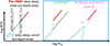 |
Fig. 1. Cartoon depicting different challenges that can arise when trying to fit the MS with no continuous and complete coverage. Current JWST surveys are very deep, but limited in size, selecting mainly low-mass galaxies. Pre-JWST surveys are not deep enough to reach such low M★. Offsets and/or changes in the slopes can make the connection between the two regimes hard to quantify if we do not consider the ensemble of both pre-JWST and JWST surveys. |
In this work we explore the MS evolution between 1 < z < 9, spanning an unprecedentedly large range of M★ and SFR, enabled by an SFR and mass-complete sample that includes sources at the low-M★ end (∼107 M⊙). This robust and cohesive dataset comprises large-area pre-JWST surveys, such as the Cosmic Assembly Near-infrared Deep Extragalactic Legacy Survey (CANDELS; Grogin et al. 2011; Koekemoer et al. 2011) and COSMOS2020 (Weaver et al. 2022), and current JWST surveys. Pre-JWST surveys allow us to probe high-M★ (> 109 M⊙), while JWST data are crucial for extending completeness to lower M★. As such, this sample allows us to probe the MS across all M★. Throughout this work we assumed ΩM, 0 = 0.3, ΩΛ, 0 = 0.7, H0 = 70 km s−1 Mpc−1, and a Chabrier (2003) initial mass function, and used AB magnitudes (Oke & Gunn 1983).
2. Data and sample selection
In this work we aim to study the evolution of the MS in the largest possible and most complete M★ and SFR range. For that purpose, we combined large-area pre-JWST surveys, which allow us to investigate the high-M★ regime (> 109 M⊙), with JWST surveys that enable the completeness to be pushed toward lower M★. The pre-JWST surveys selected in this work were CANDELS and COSMOS2020 (which sum up > 1 million galaxies), and SHARDS/CANDELS FAINT (M+23). The latter is based on image stacking and allowed us to push the limits of the former CANDELS catalog in GOODS-N toward lower M★ values. This dataset provides an independent check on the trends observed at the low-M★ end by JWST.
We selected JWST galaxies from the Cosmic Evolution Early Release Science Survey (CEERS; ERS-1345, Finkelstein et al. 2022; Bagley et al. 2023); The James Webb Space Telescope Advanced Deep Extragalactic Survey (JADES; GTO-1180, 1181, 1210, 1286, GO-1895, 1963, Eisenstein et al. 2023); The CAnadian NIRISS Unbiased Cluster/Technicolor Survey (CANUCS/Technicolor; GTO-1208, GO-3362, Willott et al. 2022; Sarrouh et al. 2026); and The Ultradeep NIRSPec and NIRCam Observations before the Epoch of Reionization survey (UNCOVER; GO-2561, Bezanson et al. 2024). A more detailed description of each of these datasets can be found in Appendix A. The final number of objects from each survey included in this work, together with some average properties, can be consulted in Table 1.
Surveys used in this work, ordered by the covered area.
To construct our parent sample, we applied several screenings to this dataset, as is outlined below. Given that some of these surveys overlap, namely JADES and CANDELS/GOODS, CEERS and CANDELS/EGS, and COSMOS2020 and CANDELS/COSMOS, we first removed potential duplicate galaxies by looking for counterparts within 0.3″ and keeping only the CANDELS sources. This guarantees a uniform treatment of overlaps, assigning them to the same parent sample, and weighting them equally in further analysis (see Sect. 3.1). SHARDS/CANDELS FAINT and CANDELS/GOODS-N also overlap and a similar process was already carried out in M+23. These duplicates constitute ∼30% of the CEERS sources and ∼10% of the JADES and COSMOS2020 galaxies, respectively.
These preliminary catalogs were then trimmed to keep galaxies with useful measurements in enough bands, considering filters covering the 0.3–8μm wavelength range, through the nbands or EAZY_nfilt flags if available, setting a ≥8 value. In addition to this cut, we required S/N ≥ 3 in at least eight bands, which is important especially when the previous flags are not available. We used the use_phot flag when available too.
For the UNCOVER and CANUCS cluster field catalogs, we restricted the gravitational lensing magnification to 1 < μ < 10, correcting SFRs, M★, and their uncertainties based on the values provided by each catalog. The redshifts, also taken from the catalogs, were restricted to 1 ≤ z ≤ 9 in every survey. These cuts left us with a parent sample of 824 287 galaxies to be fit: 613 261 from COSMOS2020; 96 948 from CANDELS; 12 696 from SHARDS/CANDELS FAINT; 10 859 from CEERS; 43 853 from JADES; 31 800 from CANUCS; and 14 870 from UNCOVER. Note that this is not our final sample, as subsequent screenings are still required. These are detailed in Sect. 3.1.
3. Physical properties
3.1. Obtaining homogeneous M★ and SFR measurements
The physical properties of each of the catalogs listed in Sect. 2 were originally computed using different fitting codes. CANDELS and SHARDS/CANDELS FAINT galaxies were fit using EAzY (Brammer et al. 2008) and pzeta (Pérez-González et al. 2005, 2008) for the photo-zs and Synthesizer (Pérez-González et al. 2005, 2008) for the stellar properties. The COSMOS2020 catalog was fit using EAzY and LePhare (Arnouts & Ilbert 2011). The CANUCS team used EAzY, Bagpipes (Carnall et al. 2018), and Dense Basis (Iyer & Gawiser 2017; Iyer et al. 2019). The UNCOVER catalog is based on EAzY and Prospector-β (Johnson et al. 2021); the one based on JADES used EAzY supplemented by flexible stellar population synthesis (FSPS; Conroy & Gunn 2010) templates; and CEERS relied on EAzY, Bagpipes, and Dense Basis.
Some of these codes did not consider the effects of outshining (Narayanan et al. 2024; Whitler et al. 2023), which can lead to systematic underestimates of the M★ (Sorba & Sawicki 2018). The latter is tightly linked to the SFH prescription, since some of them did not allow a nonparametric SFH to be set. The assumption of the priors and SFHs is more essential than the selection of the code itself. Nonparametric models capture better the variety of physical events (e.g., bursts, rejuvenation, sudden quenching, or maximally old star formation) responsible for the complex SFHs of high-z galaxies (Simha et al. 2014; Leja et al. 2019; Carvajal-Bohorquez et al. 2025).
To avoid possible systematic effects produced by combining results obtained from different configurations and codes (see Sect. 1), we opted to refit all the galaxies within our sample using Dense Basis (Iyer & Gawiser 2017; Iyer et al. 2019). This software uses nonparametric SFHs and incorporates stellar population synthesis models through the FSPS Python module. The code builds the SFHs based on the lookback times at which a galaxy assembles certain quantiles of its M★, using Gaussian processes to create smooth and flexible SFHs. It uses a flexible number of parameters, adjusted to extract the maximum amount of information from the SEDs being fit.
It is important to highlight that these are stellar fits only, and a possible AGN flux contribution is not considered. Recent studies have shown that 5–15% of galaxies at z ∼ 4 − 7 host supermassive black holes (Harikane et al. 2023; Maiolino et al. 2024). Photometric data are sometimes insufficient to confirm or dismiss the presence of AGNs, and we warn the reader that our M★ and SFR estimates may be overestimated in some of our galaxies, especially at the high-M★ end.
We built our atlas, which is a grid made up of all the parameters’ values, assuming wide ranges for the priors of the redshift, M★, and SFR, constraining the z between 0 < z < 12; M★ between 5 < log M★/M⊙ < 12; and sSFR between −12 < log sSFR[yr−1]< − 7.5, setting a flat sSFR prior. We considered the default configuration for the metallicities and a Calzetti et al. (2000) attenuation law with a flat prior for the dust. When running the code, the z was fixed to the values provided by the different catalogs (zspec when available). The atlas comprises N_pregrid = 1 000 000 templates, and we allow these to explore redshifts around ±0.1 the redshift of the galaxy.
We used point-spread function (PSF) matched photometry measured in Kron apertures (Kron 1980) for the COSMOS2020, CEERS, UNCOVER, CANUCS, and JADES objects. CANDELS photometry was also measured in Kron apertures using TFIT (Laidler et al. 2007; see also B+19). TFIT is a template-fitting code that enables one to measure galaxy photometry using prior information about the position of the sources from high-resolution observations (in this case, F160W). It creates mock PSF-matched images, computed on an object-by-object basis by smoothing the high-resolution cutouts using a convolution kernel. TFIT then fits iteratively for the photometry by comparing the real images to the models, accounting for possible contamination from nearby galaxies. SHARDS/CANDELS FAINT considers distinct apertures and resolutions and accounts for these differences through a series of aperture and offset corrections that yield results consistent with PSF-matched photometry.
The resulting Dense Basis catalogs were also screened to remove quiescent galaxies using the U, V, and J colors when provided by the photometric catalogs, and an additional sSFR cut dependent on z (log sSFR > −10 yr−1 at 1 < z < 2.5; log sSFR > −9.75 yr−1 at 2.5 < z < 3; log sSFR > −9.5 yr−1 at 3 < z < 4; and log sSFR > −9 yr−1 at z > 4). These sSFR cuts are based on a visual inspection of the SFR − M★ plane (Pearson et al. 2023). The UVJ cuts, which evolve with z, were estimated using the code presented in Antwi-Danso et al. (2023, see also Tan et al. 2025). These colors correspond to the best-fit SED colors, not corrected with the observed photometry, which can affect our selection (see Noirot et al. 2022). However, these cuts affect mainly galaxies from CANDELS and COSMOS2020 with M★ > 109 M⊙ (see red points in Fig. 6).
Moreover, we removed sources whose SFR or M★ 16th and 84th percentiles were not well constrained (i.e., were infinite or “not a number”, NaN). These cuts provided us with our final sample, made up of 755 196 galaxies. The contribution from each survey is listed in Table 1. Figures 2, 3, and 4 show the distribution in log M★, Av, and log SFR100 of the different subsamples, weighted by their surveyed area, and normalized such that the total area under the histograms is one. From now on, we shall use SFR to refer to SFR100, or SFRUV, which probes the star formation within a 100 Myr timescale, being more robust against short-term variations of the star formation. A study of burstiness, using SFR10, will be presented in Mérida et al. (in prep.).
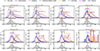 |
Fig. 2. Stellar mass histograms in different redshift intervals showing the distribution of the CANDELS (red), COSMOS2020 (maroon), SHARDS/CANDELS FAINT (green), JWST/CEERS (yellow), JADES (fuchsia), CANUCS (navy), and UNCOVER (blue) surveys. Each histogram is normalized such that the total area under the curve equals 1. The solid gray histograms in the panels underneath show the distribution of the galaxies that entered our final selection, combining the previous surveys (see Sect. 3). The 16th, 50th, and 84th percentiles for each distribution are displayed as segments, color-coded following the histograms (black for our final sample). Vertical dashed lines depict the 80% mass-completeness limit of our sample (see Sect. 3.2). |
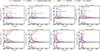 |
Fig. 3. Attenuation histograms in different redshift intervals showing the distribution of the galaxies within the distinct surveys, following the same color code as in Fig. 2. |
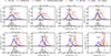 |
Fig. 4. Star formation rate histograms in different redshift intervals showing the distribution of the galaxies within the distinct surveys, following the same color code as in Fig. 2. Vertical dashed lines highlight our SFR limits (see Sect. 3.2). |
Figures 2, 3, and 4 show that CANDELS and COSMOS2020 probe high-M★ galaxies, with, on average, higher SFR. JWST surveys and SHARDS/CANDELS FAINT probe lower M★ and SFRs. While there is a smooth transition between the mass regimes dominated by JWST and pre-JWST surveys at low z, there is gradually less overlap at increasingly high z. Wider JWST surveys are essential for populating the 108.5 − 9.5 M⊙ regime at higher z, bridging the two M★ regimes. A step forward in this direction is, for instance, the MINERVA survey (Muzzin et al. 2025): an ongoing eight-filter medium-band Near Infrared Camera (NIRCam, Rieke et al. 2023a) imaging survey in the primary HST/JWST fields covering ∼548 arcmin2 of the sky.
In terms of extinction, CANDELS and COSMOS2020 display the highest values (as they also probe higher M★), although these are still small (Av < 0.5 mag). The average optical extinction of our final sample ranges from 0.2 − 0.3 mag.
Given that each catalog covers a specific M★ and SFR range, with different depths and areas, assigning equal weights to the galaxies in these surveys would lead to skewed results. As a specific example, COSMOS2020 provides ∼600 000 sources, some of them low-mass (107 − 8 M⊙). However, the catalog is not mass-complete down to those values, and hence the low-mass population included in this survey is likely very bright and made up of starbursts. On the other hand, CANUCS covers a much smaller area and provides a lower number of sources. However, the survey is much deeper, allowing us to detect not only the brightest objects at the low-mass end but also the entire population of these galaxies.
To address these differences, we selected galaxies based on the relative area covered by each survey with respect to the total area (∼2.2 deg). We considered 1 ≤ z < 1.5, 1.5 ≤ z < 2, 2 ≤ z < 2.5, 2.5 ≤ z < 3, 3 ≤ z < 4, 4 ≤ z < 5, 5 ≤ z < 7, and 7 ≤ z ≤ 9 redshift intervals, dividing the log M★ range within each interval into 0.1 dex bins. For each bin, we randomly drew N/k sources per catalog, N being the number of galaxies in the bin and k the relative area (i.e., total area/survey area, which means that every galaxy is counted multiple times, depending on the survey coverage). We verified that imposing a minimum number of galaxies per survey and bin provided similar results, given that a small number of objects in a small survey area implies a high weight in the calculations. This occurs especially at high-z and high-M★, where the number counts drop in all surveys.
In Table B.1 we show the number of objects per M★ interval and survey for each z range, as well as the contribution of each survey to the bin after weighting by the survey area. This method allows us to combine datasets with different M★ completeness levels. For instance, at 1 ≤ z < 1.5, CANDELS 80% completeness limit lies at 108.6 M⊙, but we are also selecting galaxies with 1 dex lower M★. In this case, these galaxies contribute 3% to the sample within the 107.6 − 8.0 M⊙ interval, whereas JADES + CEERS + CANUCS + UNCOVER sum up 82% of the galaxies that are being considered. The distribution of the properties of our final sample is displayed as solid gray histograms in Figs. 2, 3, and 4, and will be used to explore the MS in Sect. 4.
3.2. Completeness
3.2.1. Estimating completeness limits from observables
To derive our M★ completeness, we followed two complementary approaches. The first is based on the evolution of the number of post-starburst galaxies with M★ and z, which assumes that these galaxies are the ones prone to being missed when completeness falls toward lower M★. We created mock SEDs drawn from our Dense Basis atlas, choosing a post-starburst-like SFH, and scaling them to cover the whole M★ and z ranges. Then, we looked for galaxies in our catalogs that resemble these mock SEDs by computing cosine similarities (i.e., comparing their SED shapes) and average ratios (i.e., comparing their continuum levels). In other words, for each of these mock SEDs (i.e., per z and 0.2 dex M★ bin), we counted the number of counterparts in our catalogs. This method provides us with a selection function whose peak can be used to infer a completeness estimate at each z. However, as we move to higher z (i.e., z > 5), the S/N drops and challenges this method. For that reason, completeness at z > 5 was extrapolated from a fit to the z < 5 completeness curve, assuming that completeness decreases monotonically with z following a logarithmic trend. Further details about this method will be provided in Mérida et al. (in prep.), which will also discuss the impact of gravitational lensing in this computation. Considering the limits achieved by the JWST surveys included in this work, the average 80% M★ completeness is reached at 107.6 M⊙ at z = 1 (108.8 M⊙ at z = 9).
The second is a more traditional approach that relates our galaxy distribution with different stellar mass functions (SMFs; i.e., Santini et al. 2012; Ilbert et al. 2013; Tomczak et al. 2014; Grazian et al. 2015; Weibel et al. 2024). The ratio between the SMF and our M★ distribution allows us to define the completeness (see also M+23). At z > 5, this procedure should also be used with caution until we achieve a better understanding of the SMF at this and higher z. The method provides similar estimates to our first approach within 0.1 dex. Our dataset allows us to push traditional mass-completeness limits (e.g., CANDELS; B+19) ∼1 dex toward lower M★. We can probe 108.3 M⊙ galaxies up to z ∼ 4. This implies that we cannot reach the low-M★ regime (i.e., ≲108 M⊙) at higher z. Nevertheless, we are able to push the MS much deeper than pre-JWST MS studies at these higher z.
For the SFR completeness, we selected those bands centered at the rest-frame ultraviolet (UV) for each galaxy. The limiting magnitudes for the bands probing the spectral range around 280 nm rest-frame were translated into a UV luminosity and then into the SFR using the Kennicutt (1998) relation (M+23). Only galaxies above the M★ limits were considered, since our goal is to obtain a sample that is both M★ and SFR complete. We considered two cases: Av = 0 mag and Av equal to the median value within the corresponding z interval.
Stellar mass and SFR 80% completeness limits.
3.2.2. The underlying completeness function
Figures 2 and 4 show our M★ and SFR completeness limits as vertical lines, whose values can also be consulted in Table 2. Both limits increase with increasing z. At 1 < z < 3, the peak of the gray histograms roughly coincides with the SFR and M★ completeness limits. At higher z, the limits deviate from the peak toward higher values of both SFR and M★. The latter effect could be partially induced by the evolution in the shape of the completeness function with z.
These vertical lines were computed at the 80% level. Different levels will probe different regions of the underlying completeness function, which depends on both M★ and SFR, and evolves with z. Figure 5 shows a cartoon where we represent the M★ and SFR completeness limits as dashed lines, computed at a random x% level for illustrative purposes. The underlying function from which these limits are extracted is depicted as a solid black line. The exact parametrization of this function will be explored in detail in Mérida et al. (in prep.).
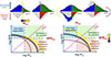 |
Fig. 5. Cartoon depicting the variations induced in the M★ (left) and SFR (right) completeness limits by changes in the shape of the completeness function (black line). We plot some hypothetical SFR and M★ limits as dashed lines. The hatched green region encloses the SFR and M★ values above both completeness limits. The hatched blue region highlights the locus of galaxies that would be detected thanks to their high SFR, but that lie below the M★ limit. The hatched orange region contains galaxies above the M★ limit that would be hard to detect because of their low SFR. The white region is occupied by galaxies that are below the M★ and SFR limits. In yellow (pink), we show how the curve should change in order to increase (decrease) both the M★ and SFR limits independently. Histograms above each panel exemplify how changes in M★ or SFR completeness would affect our final sample. Bins are color-coded according to the regions they would occupy in the log SFR−log M★ plane. We display two mirrored histograms, showing galaxies that lie above (blue and green) and below (white and red) the SFR limit. The quiescent or dormant histogram is centered at a lower M★, as bursty star formation rules at lower M★ (i.e., quiescence is not permanent and these galaxies should be included in an MS analysis). At higher M★ galaxies that fall below the MS are more prone to remain quiescent, and thus would be discarded through UVJ and sSFR cuts. Vertical and horizontal lines are color-coded following the bottom panels. The last two histograms exemplify how objects would move from the top to the mirrored histograms, and vice versa, as we change the SFR limit. |
The composite of the completeness function and the completeness limits yields four different galaxy regimes. Objects can be sufficiently massive and star-forming to exceed the M★ and SFR limits (hatched green region). Any MS or burstiness analysis should only consider these galaxies. On the other hand, there are sources that are not massive enough, but whose high SFR will make them detectable (hatched blue region). Objects that are massive enough, but have a too low SFR (hatched red region) will not be detected. Finally, there is a regime occupied by galaxies that are neither massive nor star-forming enough to be detected (white region). These last two regimes are occupied by quiescent sources, whether permanently or temporarily.
It is important to keep in mind that this is a simplified view of the parameter space. For example, some galaxies in the hatched blue region lie below the completeness curve (see the left panel of Fig. 5). Depending on the percentage used to compute the limits (the dashed horizontal line), the number of SFGs that skip our selection can increase or decrease. For illustrative purposes, we draw the completeness limits so that only galaxies in the white region fall below the line. In a realistic context, however, below the SFR completeness limits, we should expect to find a mixture of quiescent galaxies and some SFGs whose emission is too faint, and that thus remain undetected.
Figure 5 also shows the impact of the completeness shape on our datasets. We depict the effect induced in the final galaxy distribution (histograms above), which has to be complete in both SFR and M★ (green). The amount of low-mass, highly star-forming galaxies (blue) below our M★ completeness and detectable SFR will be smaller if the slope of the completeness function at lower M★ becomes steeper (yellow curve in the second panel). Understanding the completeness function in terms of both M★ and SFR is thus key to avoiding biases induced by this galaxy population (see also Simmonds et al. 2025).
On the other hand, at high redshifts, galaxies become increasingly faint, and their rest-frame UV emission is difficult to measure, which affects SFR completeness estimates. However, SFRs from these galaxies can be recovered through SED fitting, taking advantage of optical constraints.
4. The M★ versus SFR relation at low masses
Figure 6 shows M★ versus SFR of our galaxy sample as grayscale 2D histograms in the redshift intervals defined previously in Sect. 3. These two quantities exhibit a tight correlation over the examined redshift range (1 ≤ z ≤ 9). We fit the data in each panel using the locally weighted scatterplot smoothing (LOWESS) method from the Python’s statsmodels library (Seabold & Perktold 2010), which is a nonparametric method. It is based on robust locally weighted regression, not assuming any global functional form (Cleveland 1979). In this way, possible inflection points in the MS will not be artifacts due to the election of a concrete parametrization.
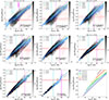 |
Fig. 6. Star formation rates versus stellar masses for our sample, divided into different redshift intervals covering 1 ≤ z ≤ 9. Galaxies are represented in gray in a 2D histogram using a symmetric logarithmic scale. In light red, we include a scatter plot (i.e., individual points) showing the galaxies that did not pass our sSFR screening. The vertical cyan lines denote the 80% mass completeness limits of our dataset. Previous limits from CANDELS are represented as vertical fuchsia lines (B+19, not corrected for outshining). The horizontal lines show our SFR limits, computed without attenuation (dashed red line) and taking the median Av of the sample in the corresponding z interval (solid red line). The LOWESS fit to the MS is shown as a thick blue line; running medians are displayed as blue circles, and the standard deviation is represented by the shaded blue region. We include four fits from the literature as dashed lines: green for Iyer et al. (2018), brown for B+19, orange for Leja et al. (2022), and pink for M+23. These fits are plotted down to their M★ completeness limits. B+19 and M+23 fits were corrected for outshining using the Sorba & Sawicki (2018) prescription. The last panel shows all our fits together, color-coded by redshift. They are displayed down to the corresponding M★ and SFR limits of the bin (see Sect. 3.2). |
We used this first LOWESS fit to carry out a sigma-clipping of the data (σ = 3) and refit the clipped distribution with LOWESS. In both iterations, we set frac = 1 (i.e., using all the data). As a result of the sigma-clipping, we removed < 1% of galaxies lying above and below the MS. Although this is a small number, we used the entire unclipped distribution to derive the MS parameters further in this section.
The fit is shown in Fig. 6 as a solid blue line. On the other hand, we also binned the whole log M★ range per z interval in 0.1 dex bins, computing the running median and scatter, also included in Fig. 6 (blue points and shaded blue region). We show the values of the running medians, the scatter, and the LOWESS fit in Table C.1.
Looking at Fig. 6, we see that at z > 5 the number of objects above our M★ and SFR completeness limits drops. This is a consequence of imposing completeness in both SFR and M★ at the same time, in the manner detailed in Sect. 3.2. More UV-continuum faint galaxies would be required to push down completeness at 5 < z < 9 (i.e., pushing down SFR completeness for this M★ limit). Additionally, wider JWST surveys are key to populating the > 109 M⊙ regime at z > 7 (i.e., pushing down M★ limits so that we reach the bulk of JWST sources; see Fig. 1). Our findings at z > 5 should thus be interpreted with caution until we can fill these gaps.
The normalization of the fits increases with z, as has been reported by previous works (e.g., Pearson et al. 2018; Popesso et al. 2023). The transition between what we call the observed low-mass regime (i.e., log M★, lim < log M★ < log M★, CANDELS, where the CANDELS limits are those reported in B+19) and the high-mass regime (i.e., log M★ > log M★, CANDELS) is smooth. The limits of the regimes are defined to account for the redshift evolution of mass completeness.
We do not see evidence of a high-M★ turnover point, but detect a bending of these fits at lower M★. We also see that the 2 < z < 2.5 and 2.5 < z < 3 fits intersect at high M★. Several factors, including the MS parametrization and binning, sSFR cuts, and the treatment of uncertainties, can produce such effects. Different parameterizations and binning can reflect statistical changes in the trends not physically motivated by the data (i.e., nonphysical inflection points, see Sect. 1). The sSFR cuts at the high-M★ end are more uncertain, as both bulge growth and AGN feedback play significant roles. We are not considering the contribution of AGN in our fits, which may induce asymmetries in the SFR uncertainties.
We included fits from previous works; namely, Iyer et al. (2018; I+18), B+19, Leja et al. (2022; L+22), and M+23. B+19 and M+23 were corrected for outshining using the Sorba & Sawicki (2018) correction; still, an offset from our relation is expected, given that this is only a general correction. I+18 is based on a previous version of Dense Basis, which could be the underlying cause of the slight offset. L+22 is based on Prospector, using a nonparametric SFH, and thus more in line with our method. Overall, taking the previous factors into account, we find a good agreement between the different fits and our estimations.
To study the variations of the MS parameters with z and M★ in more detail, we relied on three different methods. We used lmfit (Newville et al. 2014) and emcee (Foreman-Mackey et al. 2013) to run a Markov chain Monte Carlo (MCMC) sampling of the posterior distribution. For the former Python method, we assumed that the uncertainties in log M★ and log SFR are symmetrical. emcee was instead run including a split normal distribution to account for possible asymmetries in both parameters. Both methods provide compatible results when assuming symmetric uncertainties. Lastly, we computed the MS parameters using the curve_fit method from scipy.optimize (Virtanen et al. 2020). Each of these methods, which assume a linear parametrization of the MS in log–log space, provides us with values for the normalization (α), slope (β), and scatter (ϵ) of the MS. We used curve_fit to obtain an estimate of the observed or statistical MS parameters, which we then compared with the intrinsic values derived following an MCMC approach with lmfit and emcee.
Figure 7 shows our results, computed using the whole M★ regime and only considering the low-M★ regime (i.e., below the CANDELS completeness limits). The values shown in this plot can be found in Table 3. Focusing first on the estimates computed for the whole M★ regime (in black in Fig. 7), we see that the slopes derived considering asymmetric errors correspond to the lowest values. The difference between the emcee and lmfit methods is always < 0.10 at z < 5, which points to the uncertainties being overall symmetrical. The values derived using curve_fit are always larger and closer to those obtained with lmfit. The MS slope is ∼0.7 − 0.8 at least up to z ∼ 5. The scatter found by emcee is always lower than that reported by lmfit (likely because the posterior is non-Gaussian), but still compatible with the canonical values reported in Speagle et al. (2014, i.e., 0.2 − 0.3 dex) up to z ∼ 5. The pure statistical scatter values are larger by ∼0.1 dex. In Appendix D we explore the possible source for the decreasing overall scatter with z, finding that it is likely not physical but rather driven by the low-S/N SEDs at increasing z. When the S/N decreases, the posterior has a larger contribution from the prior. In Appendix D we also include the case in which only data from JWST surveys are considered, comparing with fits from the literature based on JWST, and checking the effect on the MS parameters.
 |
Fig. 7. Main sequence slope (first column) and scatter (second column) derived using the different fitting methods; namely, lmfit, assuming symmetric errors (top), emcee, considering asymmetries (middle), and scipy.optimize (bottom), fitting the data to a straight line. In each subplot, blue colors show the evolution of the parameters for the low-M★ regime (i.e., below the CANDELS M★ limits), whereas black represents our findings for the overall M★ regime. Colors are more intense up to z ∼ 5, where we have the means to explore ≲108.5 M★ objects with an SFR and mass-complete sample. At higher z, the low-M★ sample is not actually probing the physical low-M★ regime; the sample is dominated by the high-M★ end. The values here represented can be consulted in Table 3. |
Main sequence parameters.
In the low-M★ regime, the difference between the lmfit and emcee slopes is more significant. When considering asymmetric errors, we get smaller values, more in line with what was found for the whole M★ regime. A steepening of the MS could be inferred, especially looking at the lmfit method, at least up to z ∼ 5, the limit at which we can really probe the physical low-M★ regime. We estimated the level of asymmetry in the uncertainties’ distribution (i.e., how much they deviate from a Gaussian behavior) as Δxtop − Δxbottom/Δxtop + Δxbottom, with “top” being the difference between the 84th and 50th percentiles and “bottom” being the difference between the 50th and 16th percentiles. It is larger in the low-M★ regime, especially in log SFR, reaching a value of ∼ − 0.30. The latter implies that Dense Basis posteriors are skewed toward lower SFR (and also lower M★) values when fitting these low-mass sources. When taking asymmetries into account, the steepening thus becomes more subtle, highlighting the need to consider the nature of the uncertainties’ distributions when computing intrinsic parameters. In Sect. 5, we discuss the physical implications of this steepening of the MS slope at low M★.
As we move to higher z, the differences between lmfit and emcee are reduced, as we stop probing the actual low-M★ regime and asymmetries diminish. On the other hand, the values and evolution of the scatter are similar to what we found for the whole M★ regime. emcee provides lower estimates for the scatter at z < 3 at low masses, although these values lie within 0.2 − 0.3 dex.
5. Discussion
As a result of our MCMC analysis, we can neither confirm nor dismiss a possible change in the MS slope at lower M★. However, if this hint of change in the MS slope is real, the demarcation between the two different regimes, reflected by the variation in curvature of the LOWESS fits, would be located at ∼109.5 M⊙ at 1 < z < 5. Thus, this low-M★ turnover point would remind us of the turnover observed at the high-M★ end.
This same transition was identified at 108 M⊙ using the FIRE-2 zoom-in simulations in Ma et al. (2018) and observationally at 108.6 M⊙ at 6 < z < 7 in Ciesla et al. (2024). While the exact position of the turnover could vary overall, we see that its value is independent of redshift, as in M+23, where this threshold was found at 108.8 M⊙ at 1 < z < 3 with no z dependence. The lack of z dependence could point to an event in a galaxy’s lifetime that would only depend on its ability to retain gas.
This moment could match the assembly of stable disks. We now know that dynamically cold disks could be present even at very high-z (e.g., z = 7.3, Rowland et al. 2024). Dekel et al. (2020) affirmed that gas disks tend to survive only in haloes above a threshold mass of ∼2 × 10¹¹ M⊙, which would correspond to M★ ∼ 109 M⊙, with only a weak redshift dependence. According to this work, the threshold arises from the halo merger rate when accounting for the mass dependence of the ratio of galactic baryons and halo mass. The turnover at M★ ∼ 109 M⊙ corresponds to a halo mass of ∼1011 M⊙, with a weak evolution with z (Behroozi et al. 2019).
Supernova feedback is key in disrupting disks below the critical mass by driving the stellar-to-halo mass ratio that affects the merger rate, stirring up turbulence and suppressing high-angular-momentum gas supply, and confining major compactions to the critical mass (however, see Romeo & Mogotsi 2018, who argued that nearby star-forming spirals self-regulate to a quasi-universal disk stability level, showing how disk instabilities hardly correlate with M★).
Dekel et al. (2020) point out that if the M★ to baryonic mass ratio evolved with redshift, this could induce a z dependence on the critical mass mentioned above. A decrease of this quantity with z would imply a lower fraction of disks at higher redshifts at a fixed mass.
Moreover, Simons et al. (2015) found a similar turnover mass in the context of the local Tully-Fisher relation (Tully & Fisher 1977), which links M★ with the rotation velocity of galaxies. They used a morphologically blind selection of local, field emission line galaxies, finding a transition M★ in this relation at ∼109.5 M⊙. Above this critical mass, nearly all galaxies are rotation-dominated and are, on average, more morphologically disk-like. Below, the relation shows significant scatter to low rotation velocity, and galaxies can either be rotation-dominated disks or asymmetric or compact galaxies that scatter off. They refer to this transition mass as the “mass of disk formation”. Benavides et al. (2025), using the FIREbox simulation (Feldmann et al. 2023), found transition masses compatible with these values, seeing that galaxies with M★ < 109 M⊙ are rarely disk-dominated. Additionally, Ganapathy et al. (2025) characterized the asymmetry of 271 disk galaxies within CEERS at 1 < z < 4, finding that disk galaxies with lower masses (reaching down to M★ = 108.2 M⊙) tend to be more asymmetric. They measured the relation between disk galaxy asymmetry and z, finding no conclusive relationship between them.
A detailed study of the evolution of galaxy morphology with mass and redshift using JWST data could shed light on this transition, its duration, and dependencies, since the environment may also play an important role. However, it is still difficult to delve deeper into the morphology of < 109 M⊙ galaxies. Given that sources extend over smaller angular sizes, there is an increased effect from the PSF, and sources are dimmer due to cosmological dimming (Ferreira et al. 2023). Huertas-Company et al. (2024) classify the majority of low-mass galaxies in CEERS as irregulars: less bulge-dominated systems at all redshifts. As is pointed out in that same study, fluctuations in the surface brightness caused by noise can be easily interpreted as an irregular light distribution. Based also on CEERS galaxies, in this case at 1.5 < z < 6, Ferreira et al. (2023) concluded that low-mass disks (< 109 M⊙) are more likely to be peculiar galaxies with unresolved structure at all z. Deeper observations will better detect potential diffuse components around galaxies, moving some of these irregulars to the disk class.
Above this low-mass turnover mass, or “mass of disk formation”, galaxies would be fully consistent with the self-regulated evolution model, becoming massive enough to counteract feedback, and thus preventing further stochastic events. Below this threshold, galaxies are on their way to acquiring enough mass to become stable against feedback (which is powerful enough to expel the gas from the galaxies, given their low gravitational potential), developing a stable disk. The lower the M★, the more stochastic and bursty the star formation will be. The steepening in the MS slope would suggest that the SFE or the gas content is lower as we move toward lower M★. In other words, we should expect to find more galaxies in a latent phase rather than in a burst phase at progressively lower M★. The latter was probed via simulations in Gelli et al. (2023), which showed that the duty cycle gets increasingly smaller toward lower M★. In a continuation work, these findings were also compared with JWST observations, reporting consistent results (Gelli et al. 2025). At M★ < 108 M⊙, temporarily quiescent galaxies would represent the dominant population. Galaxies with 107.5 M⊙ would show a duty cycle of ∼0.6, while those with 109.0 M⊙ would show a duty cycle of 0.99, undergoing no more latent phases.
On the other hand, Hunt et al. (2020) found that dwarf star-forming local galaxies (that they define as those with M★ < 3 × 10⁹ M⊙) tend to be overwhelmed by HI accretion, so that star formation is not able to keep up with the gas supply. In galaxies with intermediate masses, which they define as 3 × 10⁹ M⊙ < M★ < 3 × 10¹⁰ M⊙ sources, star formation proceeds apace with gas availability, and HI and H2 are both proportional to SFR. These findings support the lower SFE in low-mass galaxies, and thus their rising number in latent phases as we go to a progressively lower M★ regime.
Davies et al. (2025) studied the movements of z < 1 galaxies in the sSFR−M★ plane using the Deep Extragalactic VIsible Legacy Survey (DEVILS). According to this work, low-mass sources display a mix of rapidly increasing SFHs at high sSFRs (i.e., bursty galaxies), and constant SFHs (i.e., they form stars at a constant rate, but this rate is dependent on a quantity other than just M★) that remained similar for the entirety of the life of the galaxy. They point out that a high SFR dispersion at these masses could be produced by a combination of stochastic star formation processes and galaxies with a large variation in normalization of constant SFHs. In the same line, Simmonds et al. (2025), exploring the MS using JADES data at 3 < z < 9, pointed out that shorter-term fluctuations dominate the MS scatter, although long-term variations in star formation activity are also present. Mintz et al. (2025) studied JWST/PRISM spectra of 41 low-mass (< 109 M⊙) galaxies at 1 < z < 3, many of them showing Balmer breaks. In contrast, they found that star-forming bursts occur on long timescales, ≥100 Myr, after which galaxies fall well below the MS. They also claim that, unlike what happens at low-z, high-z star-forming and dormant galaxies should be considered a unified population (i.e., the concepts of red and blue clouds, or hatched red and green regions in Fig. 5, do not apply for low-M★ and/or high-z galaxies). In other words, dormant states of galaxies are not permanent. Rather, galaxies can overcome them and enter bursty phases. Sun et al. (2023) showed that the observability of low-M★ objects is highly time-dependent when they are close to the survey’s limiting flux. As a consequence of the SFR variability, the same galaxy oscillates in and out of the observable sample. Looking for statistical samples of dormant low-M★ galaxies is key to understanding the evolution of low-M★ sources and providing better constraints on their SFHs, the MS, and other scaling relations.
To this complex picture, we should also add possible effects of AGN feedback on low-mass galaxies (Martín-Navarro & Mezcua 2018), the presence of dusty dwarfs (Bisigello et al. 2023), and the impact of galaxy mergers (Asada et al. 2023, 2024; Mérida et al. 2026), which are key in driving burstiness. Finally, the fact that the scatter we report is consistent with that found at higher M★ in the literature may suggest that the stochasticity induced by the bursty SFHs undergone by low-mass galaxies could show its imprint at lower M★ than the values probed in this work, especially as we move toward higher z. It is more likely, though, that the scatter due to the bursts may be suppressed enough that the global SFRs average out over ∼100 Myr timescales, not showing up in our results (see Simmonds et al. 2025). Caplar & Tacchella (2019) presented the scatter along the MS retrieved based on different SFR timescales and power spectrum densities, characterized by a high-frequency slope (α) and a break timescale (τbreak). Assuming bursty values for these parameters, they showed that SFR10 provides a wide ΔMS (i.e., log SFR – log SFRMS), while the SFR100 scatter remains much tighter. As the break timescales increase and α decreases (i.e., we get closer to a smooth SFH), the ΔMS values provided by both tracers become more similar. Figure 8 sketches a summary of our interpretation of the behavior of the MS in the low-M★ galaxy regime based on the previous information.
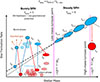 |
Fig. 8. Cartoon depicting a possible evolutionary pathway of low-M★ galaxies along the main sequence. Galaxies in a burst or star-forming phase are shown with blue colors. Those in red correspond to latent or dormant phases or quiescence (the distance of these galaxies from the main sequence can be much larger). The vertical lines denote the high-M★ turnover point from the literature (see Sect. 1) and the low-M★ turnover point reported in this work, which is z-independent. We include an M★ range that covers the different values reported from the literature and our estimates. Our value should be regarded as the end of the transition from a busty stochastic SFH to the smooth accretion mode. Below the low-M★ turnover point, the star formation is mainly driven by supernova feedback that can expel the gas from the galaxy and push it to a latent phase. Infalling gas reignites star formation again in the form of a new burst. As the galaxy assembles mass, the disk starts to form, and the galaxy becomes more stable against feedback. The number of galaxies in a latent phase increases with decreasing M★, which can be reflected in a steepening of the main-sequence slope. |
6. Summary and conclusions
In this work, we combined pre-JWST surveys (i.e., CANDELS, COSMOS2020, and SHARDS/CANDELS FAINT) with JWST surveys (i.e., CEERS, JADES, CANUCS, and UNCOVER) to examine the evolution of the main sequence at 1 ≤ z ≤ 9. This comprehensive sample allowed us to explore this scaling relation across a broad range of stellar masses and SFRs, providing insights into the inflection points that reflect the transition between the different mass regimes.
The sample, made up of 755 196 sources, was refit to obtain consistent SFRs and M★ using the Dense Basis code and a unified configuration to avoid biases, choosing a nonparametric SFH setting. This dataset allowed us to reach down to 107.6 M⊙ at z = 1 (108.8 M⊙ at z = 9) with an 80% M★ completeness, providing the means to investigate the main sequence in the low-M★ regime up to z ∼ 5 and in general up to z ∼ 9. Below the M★ and SFR limits (which must be imposed simultaneously) and toward higher z, we are more susceptible to being biased toward highly star-forming galaxies in a burst phase, while unable to select the dormant or latent population of low-M★ galaxies. Conclusions regarding the main sequence’s behavior or burstiness should be considered with caution until we can actually probe the complex SFR path traversed by low-M★ galaxies.
The MS slopes and scatter we obtain are compatible with canonical values found in the literature up to z ∼ 5 (β ∼ 0.7 − 0.8, ϵ ∼ 0.2 − 0.3 dex). When dividing the M★ range to focus on low-M★ sources, we can detect hints of a steepening of the MS slope. This effect is subtle when considering the asymmetric nature of uncertainties in this mass regime. The steepening starts at ∼109.5 M⊙, independently of redshift, which could be reflecting a critical value above which a stable disk finally assembles in galaxies. Below that mass, galaxies would be increasingly burstier and more stochastic, and likely undergo long periods of latency below the main sequence. Extending this study toward lower M★ while achieving completeness is a complex task that requires capturing galaxies in such dormant stages.
The scatter found in the low-M★ regime is also compatible with the canonical values. In this case, the use of a long-term SFR indicator may be smoothing out rapid fluctuations suffered by low-mass galaxies, fluctuations that may be better captured by shorter-timescale SFR tracers.
Acknowledgments
This research was enabled by grant 18JWST-GTO1 from the Canadian Space Agency and Discovery Grant and Discovery Accelerator funding from the Natural Sciences and Engineering Research Council (NSERC) of Canada to MS. MB acknowledges support from the ERC Grant FIRSTLIGHT, Slovenian national research agency ARIS through grants N1-0238 and P1-0188, and the program HST-GO-16667, provided through a grant from the STScI under NASA contract NAS5-26555. This research used the Canadian Advanced Network For Astronomy Research (CANFAR) platform, operated in partnership by the Canadian Astronomy Data Centre and The Digital Research Alliance of Canada with support from the National Research Council of Canada, the Canadian Space Agency, CANARIE, and the Canada Foundation for Innovation. This work is partially based on observations taken by the CANDELS Multi-Cycle Treasury Program with the NASA/ESA HST, which is operated by the Association of Universities for Research in Astronomy, Inc., under NASA contract NAS5-26555. This work is also based on observations made with the NASA/ESA/CSA James Webb Space Telescope. The data were obtained from the Mikulski Archive for Space Telescopes at the Space Telescope Science Institute, which is operated by the Association of Universities for Research in Astronomy, Inc., under NASA contract NAS 5-03127 for JWST. These observations are associated with programs ERS-1345; GTO-1180, 1181, 1210, 1286, GO-1895, 1963; GTO-1208, GO-3362; and GO-2561. This research is also based on observations collected at the European Southern Observatory under ESO programme ID 179.A-2005 and on data products produced by CALET and the Cambridge Astronomy Survey Unit on behalf of the UltraVISTA consortium.
References
- Abramson, L. E., Kelson, D. D., Dressler, A., et al. 2014, ApJ, 785, L36 [NASA ADS] [CrossRef] [Google Scholar]
- Abramson, L. E., Gladders, M. D., Dressler, A., et al. 2016, ApJ, 832, 7 [NASA ADS] [CrossRef] [Google Scholar]
- Alcalde Pampliega, B., Pérez-González, P. G., Barro, G., et al. 2019, ApJ, 876, 135 [NASA ADS] [CrossRef] [Google Scholar]
- Antwi-Danso, J., Papovich, C., Leja, J., et al. 2023, ApJ, 943, 166 [NASA ADS] [CrossRef] [Google Scholar]
- Arnouts, S., & Ilbert, O. 2011, Astrophysics Source Code Library [record ascl:1108.009] [Google Scholar]
- Arnouts, S., Walcher, C. J., Le Fèvre, O., et al. 2007, A&A, 476, 137 [CrossRef] [EDP Sciences] [Google Scholar]
- Asada, Y., Sawicki, M., Desprez, G., et al. 2023, MNRAS, 523, L40 [NASA ADS] [CrossRef] [Google Scholar]
- Asada, Y., Sawicki, M., Abraham, R., et al. 2024, MNRAS, 527, 11372 [Google Scholar]
- Atek, H., Furtak, L. J., Oesch, P., et al. 2022, MNRAS, 511, 4464 [CrossRef] [Google Scholar]
- Austin, D., Adams, N., Conselice, C. J., et al. 2023, ApJ, 952, L7 [NASA ADS] [CrossRef] [Google Scholar]
- Bagley, M. B., Finkelstein, S. L., Koekemoer, A. M., et al. 2023, ApJ, 946, L12 [NASA ADS] [CrossRef] [Google Scholar]
- Barro, G., Pérez-González, P. G., Cava, A., et al. 2019, ApJS, 243, 22 [NASA ADS] [CrossRef] [Google Scholar]
- Behroozi, P., Wechsler, R. H., Hearin, A. P., & Conroy, C. 2019, MNRAS, 488, 3143 [NASA ADS] [CrossRef] [Google Scholar]
- Benavides, J. A., Sales, L. V., Wetzel, A., et al. 2025, MNRAS, e-prints [arXiv:2508.00991] [Google Scholar]
- Bezanson, R., Labbe, I., Whitaker, K. E., et al. 2024, ApJ, 974, 92 [NASA ADS] [CrossRef] [Google Scholar]
- Bisigello, L., Gandolfi, G., Grazian, A., et al. 2023, A&A, 676, A76 [NASA ADS] [CrossRef] [EDP Sciences] [Google Scholar]
- Boogaard, L. A., Brinchmann, J., Bouché, N., et al. 2018, A&A, 619, A27 [NASA ADS] [CrossRef] [EDP Sciences] [Google Scholar]
- Brammer, G. B., van Dokkum, P. G., & Coppi, P. 2008, ApJ, 686, 1503 [Google Scholar]
- Broussard, A., Gawiser, E., Iyer, K., et al. 2019, ApJ, 873, 74 [Google Scholar]
- Cairós, L. M., Caon, N., Zurita, C., et al. 2010, A&A, 520, A90 [NASA ADS] [CrossRef] [EDP Sciences] [Google Scholar]
- Calzetti, D., Armus, L., Bohlin, R. C., et al. 2000, ApJ, 533, 682 [NASA ADS] [CrossRef] [Google Scholar]
- Caplar, N., & Tacchella, S. 2019, MNRAS, 487, 3845 [NASA ADS] [CrossRef] [Google Scholar]
- Caputi, K. I., Caminha, G. B., Fujimoto, S., et al. 2021, ApJ, 908, 146 [NASA ADS] [CrossRef] [Google Scholar]
- Carnall, A. C., McLure, R. J., Dunlop, J. S., & Davé, R. 2018, MNRAS, 480, 4379 [Google Scholar]
- Carvajal-Bohorquez, C., Ciesla, L., Laporte, N., et al. 2025, A&A, 704, A290 [NASA ADS] [CrossRef] [EDP Sciences] [Google Scholar]
- Chabrier, G. 2003, PASP, 115, 763 [Google Scholar]
- Ciesla, L., Elbaz, D., Ilbert, O., et al. 2024, A&A, 686, A128 [NASA ADS] [CrossRef] [EDP Sciences] [Google Scholar]
- Cirasuolo, M., McLure, R. J., Dunlop, J. S., et al. 2007, MNRAS, 380, 585 [NASA ADS] [CrossRef] [Google Scholar]
- Clarke, L., Shapley, A. E., Sanders, R. L., et al. 2024, ApJ, 977, 133 [NASA ADS] [CrossRef] [Google Scholar]
- Cleveland, W. S. 1979, J. Am. Stat. Assoc., 74, 829 [Google Scholar]
- Cole, J. W., Papovich, C., Finkelstein, S. L., et al. 2025, ApJ, 979, 193 [Google Scholar]
- Conroy, C., & Gunn, J. E. 2010, Astrophysics Source Code Library [record ascl:1010.043] [Google Scholar]
- Daddi, E., Dickinson, M., Morrison, G., et al. 2007, ApJ, 670, 156 [NASA ADS] [CrossRef] [Google Scholar]
- Davies, L. J. M., Thorne, J. E., Bellstedt, S., et al. 2025, MNRAS, 541, 573 [Google Scholar]
- Davis, M., Guhathakurta, P., Konidaris, N. P., et al. 2007, ApJ, 660, L1 [NASA ADS] [CrossRef] [Google Scholar]
- Dekel, A., Ginzburg, O., Jiang, F., et al. 2020, MNRAS, 493, 4126 [CrossRef] [Google Scholar]
- D’Eugenio, F., Maiolino, R., Mahatma, V. H., et al. 2025, MNRAS, 536, 51 [Google Scholar]
- Dickinson, M., Bergeron, J., Casertano, S., et al. 2003, Great Observatories Origins Deep Survey (GOODS) Validation Observations, Spitzer Proposal ID 196 [Google Scholar]
- Domínguez, A., Siana, B., Brooks, A. M., et al. 2015, MNRAS, 451, 839 [CrossRef] [Google Scholar]
- Doyon, R., Willott, C. J., Hutchings, J. B., et al. 2023, PASP, 135, 098001 [NASA ADS] [CrossRef] [Google Scholar]
- Dunne, L., Ivison, R. J., Maddox, S., et al. 2009, MNRAS, 394, 3 [NASA ADS] [CrossRef] [Google Scholar]
- Eisenstein, D. J., Willott, C., Alberts, S., et al. 2023, ApJS, accepted [arXiv:2306.02465] [Google Scholar]
- Eisenstein, D. J., Johnson, B. D., Robertson, B., et al. 2025, ApJS, 281, 50 [Google Scholar]
- Elbaz, D., Dickinson, M., Hwang, H. S., et al. 2011, A&A, 533, A119 [NASA ADS] [CrossRef] [EDP Sciences] [Google Scholar]
- Emami, N., Siana, B., Weisz, D. R., et al. 2019, ApJ, 881, 71 [NASA ADS] [CrossRef] [Google Scholar]
- Feldmann, R., Quataert, E., Faucher-Giguère, C.-A., et al. 2023, MNRAS, 522, 3831 [NASA ADS] [CrossRef] [Google Scholar]
- Ferreira, L., Conselice, C. J., Sazonova, E., et al. 2023, ApJ, 955, 94 [NASA ADS] [CrossRef] [Google Scholar]
- Finkelstein, S. L., Dickinson, M., Ferguson, H. C., et al. 2017, The Cosmic Evolution Early Release Science (CEERS) Survey, JWST Proposal ID 1345. Cycle 0 Early Release Science [Google Scholar]
- Finkelstein, S. L., Bagley, M. B., Arrabal Haro, P., et al. 2022, ApJ, 940, L55 [NASA ADS] [CrossRef] [Google Scholar]
- Finkelstein, S. L., Bagley, M. B., Arrabal Haro, P., et al. 2025, ApJ, 983, L4 [Google Scholar]
- Flores Velázquez, J. A., Gurvich, A. B., Faucher-Giguère, C.-A., et al. 2021, MNRAS, 501, 4812 [CrossRef] [Google Scholar]
- Foreman-Mackey, D., Hogg, D. W., Lang, D., & Goodman, J. 2013, PASP, 125, 306 [Google Scholar]
- Galametz, A., Grazian, A., Fontana, A., et al. 2013, ApJS, 206, 10 [Google Scholar]
- Ganapathy, A., Petersen, M. S., Yaaqib, R., & Filion, C. 2025, MNRAS, 539, 661 [Google Scholar]
- Gelli, V., Salvadori, S., Ferrara, A., Pallottini, A., & Carniani, S. 2023, ApJ, 954, L11 [NASA ADS] [CrossRef] [Google Scholar]
- Gelli, V., Pallottini, A., Salvadori, S., et al. 2025, ApJ, 985, 126 [Google Scholar]
- Giavalisco, M., Ferguson, H. C., Koekemoer, A. M., et al. 2004, ApJ, 600, L93 [NASA ADS] [CrossRef] [Google Scholar]
- Grazian, A., Fontana, A., Santini, P., et al. 2015, A&A, 575, A96 [NASA ADS] [CrossRef] [EDP Sciences] [Google Scholar]
- Grogin, N. A., Kocevski, D. D., Faber, S. M., et al. 2011, ApJS, 197, 35 [NASA ADS] [CrossRef] [Google Scholar]
- Guo, Y., Ferguson, H. C., Giavalisco, M., et al. 2013, ApJS, 207, 24 [NASA ADS] [CrossRef] [Google Scholar]
- Hainline, K. N., Johnson, B. D., Robertson, B., et al. 2024, ApJ, 964, 71 [CrossRef] [Google Scholar]
- Harikane, Y., Zhang, Y., Nakajima, K., et al. 2023, ApJ, 959, 39 [NASA ADS] [CrossRef] [Google Scholar]
- Harshan, A., Bradač, M., Abraham, R., et al. 2024, MNRAS, 532, 1112 [NASA ADS] [CrossRef] [Google Scholar]
- Huertas-Company, M., Iyer, K. G., Angeloudi, E., et al. 2024, A&A, 685, A48 [NASA ADS] [CrossRef] [EDP Sciences] [Google Scholar]
- Hunt, L. K., Tortora, C., Ginolfi, M., & Schneider, R. 2020, A&A, 643, A180 [NASA ADS] [CrossRef] [EDP Sciences] [Google Scholar]
- Ilbert, O., McCracken, H. J., Le Fèvre, O., et al. 2013, A&A, 556, A55 [NASA ADS] [CrossRef] [EDP Sciences] [Google Scholar]
- Iyer, K., & Gawiser, E. 2017, ApJ, 838, 127 [NASA ADS] [CrossRef] [Google Scholar]
- Iyer, K., Gawiser, E., Davé, R., et al. 2018, ApJ, 866, 120 [Google Scholar]
- Iyer, K. G., Gawiser, E., Faber, S. M., et al. 2019, ApJ, 879, 116 [NASA ADS] [CrossRef] [Google Scholar]
- Jakobsen, P., Ferruit, P., Alves de Oliveira, C., et al. 2022, A&A, 661, A80 [NASA ADS] [CrossRef] [EDP Sciences] [Google Scholar]
- Johnson, B. D., Leja, J., Conroy, C., & Speagle, J. S. 2021, ApJS, 254, 22 [NASA ADS] [CrossRef] [Google Scholar]
- Joshi, R., Das, S., Fumagalli, M., et al. 2025, A&A, 695, A206 [NASA ADS] [CrossRef] [EDP Sciences] [Google Scholar]
- Kashino, D., Silverman, J. D., Rodighiero, G., et al. 2013, ApJ, 777, L8 [Google Scholar]
- Kennicutt, R. C., Jr. 1989, ApJ, 344, 685 [Google Scholar]
- Kennicutt, R. C., Jr. 1998, ARA&A, 36, 189 [Google Scholar]
- Koekemoer, A. M., Faber, S. M., Ferguson, H. C., et al. 2011, ApJS, 197, 36 [NASA ADS] [CrossRef] [Google Scholar]
- Kron, R. G. 1980, ApJS, 43, 305 [Google Scholar]
- Laidler, V. G., Papovich, C., Grogin, N. A., et al. 2007, PASP, 119, 1325 [Google Scholar]
- Lawrence, A., Warren, S. J., Almaini, O., et al. 2007, MNRAS, 379, 1599 [Google Scholar]
- Lee, N., Sanders, D. B., Casey, C. M., et al. 2015, ApJ, 801, 80 [Google Scholar]
- Leja, J., Carnall, A. C., Johnson, B. D., Conroy, C., & Speagle, J. S. 2019, ApJ, 876, 3 [Google Scholar]
- Leja, J., Speagle, J. S., Ting, Y.-S., et al. 2022, ApJ, 936, 165 [NASA ADS] [CrossRef] [Google Scholar]
- Leslie, S. K., Kewley, L. J., Sanders, D. B., & Lee, N. 2016, MNRAS, 455, L82 [NASA ADS] [CrossRef] [Google Scholar]
- Lilly, S. J., Carollo, C. M., Pipino, A., Renzini, A., & Peng, Y. 2013, ApJ, 772, 119 [NASA ADS] [CrossRef] [Google Scholar]
- Lin, X., Cai, Z., Zou, S., et al. 2023, ApJ, 944, L59 [NASA ADS] [CrossRef] [Google Scholar]
- Lofthouse, E. K., Fumagalli, M., Fossati, M., et al. 2020, MNRAS, 491, 2057 [NASA ADS] [CrossRef] [Google Scholar]
- Looser, T. J., D’Eugenio, F., Arribas, S., et al. 2024a, OASIS: Observing All phases of StochastIc Star formation – A census of galaxies at z = 5–8 over the entire SFR–M? plane, JWST Proposal. Cycle 3, ID. #5997 [Google Scholar]
- Looser, T. J., D’Eugenio, F., Maiolino, R., et al. 2024b, Nature, 629, 53 [Google Scholar]
- Lorenzo, M., Garcia, M., Najarro, F., et al. 2022, MNRAS, 516, 4164 [NASA ADS] [CrossRef] [Google Scholar]
- Ma, X., Hopkins, P. F., Garrison-Kimmel, S., et al. 2018, MNRAS, 478, 1694 [NASA ADS] [CrossRef] [Google Scholar]
- Maiolino, R., Scholtz, J., Curtis-Lake, E., et al. 2024, A&A, 691, A145 [NASA ADS] [CrossRef] [EDP Sciences] [Google Scholar]
- Malmquist, K. G. 1922, Meddelanden fran Lunds Astronomiska Observatorium Serie I, 100, 1 [Google Scholar]
- Martín-Navarro, I., & Mezcua, M. 2018, ApJ, 855, L20 [NASA ADS] [CrossRef] [Google Scholar]
- Maseda, M. V., van der Wel, A., Rix, H.-W., et al. 2014, ApJ, 791, 17 [CrossRef] [Google Scholar]
- Matthee, J., & Schaye, J. 2019, MNRAS, 484, 915 [CrossRef] [Google Scholar]
- Mérida, R. M., Pérez-González, P. G., Sánchez-Blázquez, P., et al. 2023, ApJ, 950, 125 [CrossRef] [Google Scholar]
- Mérida, R. M., Gómez-Guijarro, C., Pérez-González, P. G., et al. 2024, A&A, 686, A64 [NASA ADS] [CrossRef] [EDP Sciences] [Google Scholar]
- Mérida, R. M., Gaspar, G., Asada, Y., et al. 2026, A&A, in press, https://doi.org/10.1051/0004-6361/202557594 [Google Scholar]
- Merlin, E., Santini, P., Paris, D., et al. 2024, A&A, 691, A240 [NASA ADS] [CrossRef] [EDP Sciences] [Google Scholar]
- Mintz, A., Setton, D. J., Greene, J. E., et al. 2025, ApJ, submitted [arXiv:2506.16510] [Google Scholar]
- Muzzin, A., Marchesini, D., Suess, K., et al. 2025, MINERVA: Unlocking the Hidden Gems of the Distant Universe and Completing HST and JWST?s Imaging Legacy with Medium Bands, JWST Proposal. Cycle 4, ID. #7814 [Google Scholar]
- Narayanan, D., Lower, S., Torrey, P., et al. 2024, ApJ, 961, 73 [NASA ADS] [CrossRef] [Google Scholar]
- Nayyeri, H., Hemmati, S., Mobasher, B., et al. 2017, ApJS, 228, 7 [NASA ADS] [CrossRef] [Google Scholar]
- Newville, M., Stensitzki, T., Allen, D. B., & Ingargiola, A. 2014, https://doi.org/10.5281/zenodo.11813 [Google Scholar]
- Noeske, K. G., Weiner, B. J., Faber, S. M., et al. 2007, ApJ, 660, L43 [CrossRef] [Google Scholar]
- Noirot, G., Sawicki, M., Abraham, R., et al. 2022, MNRAS, 512, 3566 [NASA ADS] [CrossRef] [Google Scholar]
- Oke, J. B., & Gunn, J. E. 1983, ApJ, 266, 713 [NASA ADS] [CrossRef] [Google Scholar]
- Pearson, W. J., Wang, L., Hurley, P. D., et al. 2018, A&A, 615, A146 [NASA ADS] [CrossRef] [EDP Sciences] [Google Scholar]
- Pearson, W. J., Pistis, F., Figueira, M., et al. 2023, A&A, 679, A35 [NASA ADS] [CrossRef] [EDP Sciences] [Google Scholar]
- Pérez-González, P. G., Rieke, G. H., Egami, E., et al. 2005, ApJ, 630, 82 [Google Scholar]
- Pérez-González, P. G., Rieke, G. H., Villar, V., et al. 2008, ApJ, 675, 234 [Google Scholar]
- Pérez-González, P. G., Cava, A., Barro, G., et al. 2013, ApJ, 762, 46 [Google Scholar]
- Popesso, P., Concas, A., Cresci, G., et al. 2023, MNRAS, 519, 1526 [Google Scholar]
- Reddy, N. A., Pettini, M., Steidel, C. C., et al. 2012, ApJ, 754, 25 [Google Scholar]
- Rieke, G. H., Wright, G. S., Böker, T., et al. 2015, PASP, 127, 584 [NASA ADS] [CrossRef] [Google Scholar]
- Rieke, M. J., Kelly, D. M., Misselt, K., et al. 2023a, PASP, 135, 028001 [CrossRef] [Google Scholar]
- Rieke, M. J., Robertson, B., Tacchella, S., et al. 2023b, ApJS, 269, 16 [NASA ADS] [CrossRef] [Google Scholar]
- Rinaldi, P., Caputi, K. I., van Mierlo, S. E., et al. 2022, ApJ, 930, 128 [NASA ADS] [CrossRef] [Google Scholar]
- Rinaldi, P., Navarro-Carrera, R., Caputi, K. I., et al. 2025, ApJ, 981, 161 [Google Scholar]
- Romeo, A. B., & Mogotsi, K. M. 2018, MNRAS, 480, L23 [NASA ADS] [CrossRef] [Google Scholar]
- Rowland, L. E., Hodge, J., Bouwens, R., et al. 2024, MNRAS, 535, 2068 [Google Scholar]
- Santini, P., Fontana, A., Grazian, A., et al. 2012, A&A, 538, A33 [NASA ADS] [CrossRef] [EDP Sciences] [Google Scholar]
- Santini, P., Fontana, A., Castellano, M., et al. 2017, ApJ, 847, 76 [NASA ADS] [CrossRef] [Google Scholar]
- Sarrouh, G. T. E., Asada, Y., Martis, N. S., et al. 2026, ApJS, 282, 3 [Google Scholar]
- Sawicki, M. 2012, MNRAS, 421, 2187 [Google Scholar]
- Sawicki, M., Arnouts, S., Huang, J., et al. 2019, MNRAS, 489, 5202 [NASA ADS] [Google Scholar]
- Schmidt, M. 1959, ApJ, 129, 243 [NASA ADS] [CrossRef] [Google Scholar]
- Schreiber, C., Pannella, M., Elbaz, D., et al. 2015, A&A, 575, A74 [NASA ADS] [CrossRef] [EDP Sciences] [Google Scholar]
- Scoville, N., Aussel, H., Brusa, M., et al. 2007, ApJS, 172, 1 [Google Scholar]
- Seabold, S., & Perktold, J. 2010, in 9th Python in Science Conference [Google Scholar]
- Simha, V., Weinberg, D. H., Conroy, C., et al. 2014, MNRAS, submitted [arXiv:1404.0402] [Google Scholar]
- Simmonds, C., Tacchella, S., McClymont, W., et al. 2025, MNRAS, 544, 4551 [Google Scholar]
- Simons, R. C., Kassin, S. A., Weiner, B. J., et al. 2015, MNRAS, 452, 986 [Google Scholar]
- Smith, F. M., & Thacker, R. J. 2024, MNRAS, 532, 4774 [Google Scholar]
- Sorba, R., & Sawicki, M. 2018, MNRAS, 476, 1532 [NASA ADS] [CrossRef] [Google Scholar]
- Speagle, J. S., Steinhardt, C. L., Capak, P. L., & Silverman, J. D. 2014, ApJS, 214, 15 [Google Scholar]
- Stefanon, M., Yan, H., Mobasher, B., et al. 2017, ApJS, 229, 32 [NASA ADS] [CrossRef] [Google Scholar]
- Stinson, G. S., Dalcanton, J. J., Quinn, T., Kaufmann, T., & Wadsley, J. 2007, ApJ, 667, 170 [NASA ADS] [CrossRef] [Google Scholar]
- Strait, V., Brammer, G., Muzzin, A., et al. 2023, ApJ, 949, L23 [NASA ADS] [CrossRef] [Google Scholar]
- Suess, K. A., Weaver, J. R., Price, S. H., et al. 2024, ApJ, 976, 101 [Google Scholar]
- Sun, F., Egami, E., Pérez-González, P. G., et al. 2021, ApJ, 922, 114 [NASA ADS] [CrossRef] [Google Scholar]
- Sun, G., Faucher-Giguère, C.-A., Hayward, C. C., & Shen, X. 2023, MNRAS, 526, 2665 [NASA ADS] [CrossRef] [Google Scholar]
- Szalay, A. S., Connolly, A. J., & Szokoly, G. P. 1999, AJ, 117, 68 [Google Scholar]
- Tacchella, S., Dekel, A., Carollo, C. M., et al. 2016, MNRAS, 457, 2790 [Google Scholar]
- Tan, V. Y. Y., Muzzin, A., Sarrouh, G. T. E., et al. 2025, ApJ, 994, 94 [Google Scholar]
- Tomczak, A. R., Quadri, R. F., Tran, K.-V. H., et al. 2014, ApJ, 783, 85 [Google Scholar]
- Tomczak, A. R., Quadri, R. F., Tran, K.-V. H., et al. 2016, ApJ, 817, 118 [Google Scholar]
- Treu, T., Roberts-Borsani, G., Bradac, M., et al. 2022, ApJ, 935, 110 [NASA ADS] [CrossRef] [Google Scholar]
- Tully, R. B., & Fisher, J. R. 1977, A&A, 54, 661 [NASA ADS] [Google Scholar]
- Virtanen, P., Gommers, R., Oliphant, T. E., et al. 2020, Nat. Methods, 17, 261 [Google Scholar]
- Wang, T.-M., Magnelli, B., Schinnerer, E., et al. 2024, A&A, 681, A110 [NASA ADS] [CrossRef] [EDP Sciences] [Google Scholar]
- Weaver, J. R., Kauffmann, O. B., Ilbert, O., et al. 2022, ApJS, 258, 11 [NASA ADS] [CrossRef] [Google Scholar]
- Weaver, J. R., Cutler, S. E., Pan, R., et al. 2024, ApJS, 270, 7 [NASA ADS] [CrossRef] [Google Scholar]
- Weibel, A., Oesch, P. A., Barrufet, L., et al. 2024, MNRAS, 533, 1808 [NASA ADS] [CrossRef] [Google Scholar]
- Whitaker, K. E., Labbé, I., van Dokkum, P. G., et al. 2011, ApJ, 735, 86 [Google Scholar]
- Whitaker, K. E., van Dokkum, P. G., Brammer, G., & Franx, M. 2012, ApJ, 754, L29 [Google Scholar]
- Whitaker, K. E., Franx, M., Leja, J., et al. 2014, ApJ, 795, 104 [NASA ADS] [CrossRef] [Google Scholar]
- Whitler, L., Stark, D. P., Endsley, R., et al. 2023, MNRAS, 519, 5859 [NASA ADS] [CrossRef] [Google Scholar]
- Williams, R. J., Quadri, R. F., Franx, M., van Dokkum, P., & Labbé, I. 2009, ApJ, 691, 1879 [NASA ADS] [CrossRef] [Google Scholar]
- Willott, C. J., Doyon, R., Albert, L., et al. 2022, PASP, 134, 025002 [CrossRef] [Google Scholar]
- Wolfe, A. M., Gawiser, E., & Prochaska, J. X. 2005, ARA&A, 43, 861 [NASA ADS] [CrossRef] [Google Scholar]
- Zhou, L., Elbaz, D., Franco, M., et al. 2020, A&A, 642, A155 [NASA ADS] [CrossRef] [EDP Sciences] [Google Scholar]
Appendix A: Survey descriptions
In this appendix we provide more details about the surveys being combined in this work.
A.1. CANDELS
CANDELS is a 902-orbit HST Multi-Cycle Treasury program that combined previously obtained multi-wavelength data, including Advanced Camera for Surveys (ACS) optical observations, with new Wide Field Camera 3 (WFC3) near infrared (NIR) images. The project comprises five sky fields: the Great Observatories Origins Deep Survey fields (GOODS-N and GOODS-S, Dickinson et al. 2003, Giavalisco et al. 2004), the UKIDSS Ultradeep Survey field (UDS, Lawrence et al. 2007, Cirasuolo et al. 2007), the Extended Groth Strip (EGS, Davis et al. 2007), and the Cosmological Evolution Survey field (COSMOS, Scoville et al. 2007).
The exploitation of these data yielded multi-wavelength photometric catalogs, spanning from the UV to the far infrared, for each of these fields (Guo et al. 2013 for GOODS-S; Galametz et al. 2013 for UDS; Nayyeri et al. 2017 for COSMOS; Stefanon et al. 2017 for EGS; and B+19 for GOODS-N). The CANDELS source selection was based on the emission in the F160W NIR filter. These observations enabled the detection of over 250,000 galaxies.
A.2. COSMOS2020
The COSMOS2020 catalog comprises 1.7 million galaxies across the 2 deg2 of the COSMOS field, ∼966,000 of them measured with all available broad-band data. COSMOS2020 adds deeper optical and NIR images from the Subaru Hyper Suprime-Cam and VISTA Infrared Camera surveys, as well as the definitive reprocessing of all Spitzer data ever taken on COSMOS. It also includes all archival MegaCam COSMOS U data, recombined in addition to new data taken as part of the Canada France Hawaii Telescope Large Area U-band Deep Survey (CLAUDS, Sawicki et al. 2019). Source selection in this survey was carried out on a chi-squared izYJHKs image (Szalay et al. 1999).
A.3. SHARDS/CANDELS FAINT
The SHARDS/CANDELS FAINT catalog (M+23) consists of 34,061 ultra-faint (27 < i < 30 mag) galaxies at 1 < z < 3 detected in the GOODS-N field. The sample was built by stacking the 25 ultra-deep medium-band images gathered by the Gran Telescopio de Canarias Survey for High-z Absorption Red and Dead Sources project (GTC/SHARDS; Pérez-González et al. 2013) as well as the ACS broad-band observations from CANDELS. SHARDS obtained data in 25 medium-band filters in the 500–950 nm spectral range, reaching at least magnitude 26.5 at the 5σ level at subarcsecond seeing in each one and providing a spectral resolution of R = 50 in the optical.
A.4. CEERS
The Cosmic Evolution Early Release Science Survey (CEERS; ERS-1345, Finkelstein et al. 2017, Finkelstein et al. 2022, Bagley et al. 2023, Finkelstein et al. 2025) is a 77.2 hrs Director’s Discretionary Early Release Science Program that consists of NIRCam and Mid-Infrared Instrument (MIRI, Rieke et al. 2015) imaging, Near Infrared Spectrograph (NIRSpec, Jakobsen et al. 2022) low (R ∼100) and medium (R ∼1000) resolution spectroscopy, and NIRCam slitless grism (R ∼1500) spectroscopy. It targeted the HST-observed region of EGS, supported by a rich set of multiwavelength observations. Specifically, this survey counts on NIRCam imaging in six broadband filters (F115W, F150W, F200W, F277W, F356W, and F444W) and one medium-band filter (F410M) over four pointings, obtained in parallel with primary MIRI observations. Source identification was based on the emission in the F277W NIRCam band. The CEERS photometric catalog contains ∼100, 000 galaxies (Merlin et al. 2024).
A.5. JADES
The James Webb Space Telescope Advanced Deep Extragalactic Survey (JADES; GTO-1180, 1181, 1210, 1286, GO-1895, 1963, Eisenstein et al. 2023) is a program of infrared imaging and spectroscopy in the GOODS-S and GOODS-N deep fields, designed to study galaxy evolution from high z to cosmic noon. It uses ∼770 hrs of Cycle 1 NIRCam and NIRSpec guaranteed time. In GOODS-S, in and around the Hubble Ultra Deep Field and Chandra Deep Field South, JADES produced a deep imaging region of ∼45 arcmin2 (average of 130 hrs of exposure time spread over 9 NIRCam filters). This is extended at medium depth in GOODS-S and GOODS-N with NIRCam imaging of ∼175 arcmin2 (average exposure time of 20 hrs spread over 8 − 10 filters). Both fields were characterized with NIRSpec multi-object spectroscopy and coordinated MIRI parallels. Source detection was based on an inverse-variance-weighted stack of the NIRCam F277W, F335M, F356W, F410M, and F444W images, which led to the identification of ∼170, 000 galaxies. In this work, we used the GOODS-S-Deep v2.0 and GOODS-N v1.0 catalogs (Rieke et al. 2023b, Hainline et al. 2024, Eisenstein et al. 2025).
A.6. CANUCS
The CAnadian NIRISS Unbiased Cluster Survey (CANUCS; GTO-1208, Willott et al. 2022) is a JWST Cycle 1 GTO program targeting 5 lensing clusters and their adjacent flanking fields in parallel (Abell 370, MACS0416, MACS0417, MACS1149, MACS1423), with a total surveyed area of ∼100 arcmin2. This project combines NIRCam imaging, Near InfraRed Imager and Slitless Spectrograph (NIRISS, Doyon et al. 2023) slitless spectroscopy, and NIRSpec prism multi-object spectroscopy. It also includes Technicolor data (TEC; GO-3362, PI: Muzzin): a Cycle 2 follow-up GO program targeting 3 of the CANUCS clusters (Abell 370, MACS0416, MACS1149). Technicolor provides slitless spectroscopy with NIRISS in F090W to the cluster fields, while adding 8 wide, medium, and narrow band filters to the flanking fields. Source detection was based on a deep χmean detection image, created by co-adding background-subtracted images for all available JWST and HST-optical filters in each field. This method enabled the identification of ∼121, 000 galaxies (Sarrouh et al. 2026).
A.7. UNCOVER
The Ultradeep NIRSPec and NIRCam Observations before the Epoch of Reionization survey (UNCOVER; GO-2561, Bezanson et al. 2024) is a Cycle 1 JWST Treasury program that includes ultradeep imaging of ∼45 arcmin2 on and around the Abell 2744 galaxy cluster, with follow-up on ∼500 galaxies with NIRSpec/PRISM. The latest data release catalog ("SUPER", Weaver et al. 2024) was built from a selection based on a long-wavelength F277W+F356W+F444W detection image with photometry measured on the 27 available HST and JWST bands over 56 arcmin2. These data are enriched with several major surveys, including MegaScience (Suess et al. 2024) and GLASS (Treu et al. 2022). The UNCOVER source catalog contains ∼70, 000 galaxies.
Appendix B: M★ binning and weighting
In Table B.1, we show the number of galaxies per survey considered within each log M★ interval and redshift range. We include the weight of each survey in the overall counts.
log M★ binning per survey and redshift interval.
Appendix C: Main sequence fit values
In Table C.1, we include the running medians, statistical scatter, and the LOWESS MS fit, presented in Sect. 4.
Running medians, statistical scatter, and values of our LOWESS fit.
Appendix D: Main sequence tests
In Sect. 4, we report values of the MS scatter that decrease with increasing redshift. Although these estimates lie within the canonical values, in this appendix we explore the possible underlying causes for this trend. We also show a fit based only on JWST data, excluding CANDELS, SHARDS/CANDELS FAINT, and COSMOS2020.
Evolution of the Main Sequence slopes and scatter with redshift in the global and low-M★ regimes that result when applying an S/N cut.
D.1. S/N test
We selected those galaxies with a S/N > 50 in five or more bands. This is a very restrictive cut, which allowed us to select only those galaxies with very robust individual measurements from Dense Basis. We repeated the analysis described in Sect. 4, weighting by the survey area as detailed in Sect. 3, and show the corresponding MS fits in Fig. D.1. The values of the slopes and scatter are included in Table D.1.
Looking at Fig. D.1, we see how the low-mass galaxies that pass this screening are those with the highest SFRs. This translates into a flattening of the MS (yellow line), which reflects a selection effect, even though the global sample is mass complete at those M★. The latter highlights the need to provide accurate and realistic estimates for completeness in this kind of study, based on the final screened samples (see also Simmonds et al. 2025).
If we now focus on Table D.1 and the values retrieved for the scatter for all the galaxies, we can see that these are consistent with 0.3 dex. They do not evolve with z up to z ∼ 5, above which this S/N cut resembles the different screening processes applied in Sect. and 3, ending up with a similar selection.
D.2. JWST data only
In this appendix we include the MS fits derived using only JWST observations, namely data from CEERS, JADES, CANUCS, and UNCOVER. These fits are shown in Fig. D.1 (pink line), where we also depict the fits from Rinaldi et al. (2022) and Clarke et al. (2024), which probe z > 3 galaxies.
Examining the evolution of the fits based just on JWST data at z < 3, we see that they lie below the MS fits computed using the whole sample. The final panel includes all these fits, and we can see how the slopes, especially at 1 ≤ z ≤ 2, get flatter in the low-M★ regime, contrary to what we find using the whole sample. This illustrates the challenges shown in Fig. 1 in fitting the MS when lacking a comprehensive M★ and SFR coverage, and thus in understanding the evolution of the MS parameters. At higher z, the contribution from JWST surveys to the number counts is larger, resulting in similar results to those described in Sect. 4.
Examining the evolution of the fits from Rinaldi et al. (2022) and Clarke et al. (2024), we see that their slopes become increasingly flatter. At z > 5, the fits fall below our SFR and M★ limits, pointing to potential selection effects.
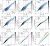 |
Fig. D.1. Star formation rates versus stellar masses divided into different redshift intervals covering 1 < z < 9. The 2D histograms represented here correspond only to the JWST data. The LOWESS fit to the main sequence described in Sect. 4 is shown in blue; in yellow, we include the MS fit using only those galaxies with S/N > 50 in at least five bands; in pink, we show the fits derived using only JWST data. We include two fits to the MS from the literature as dashed lines: lime for Rinaldi et al. 2022 and orange for Clarke et al. 2024. |
All Tables
Evolution of the Main Sequence slopes and scatter with redshift in the global and low-M★ regimes that result when applying an S/N cut.
All Figures
|
Fig. 1. Cartoon depicting different challenges that can arise when trying to fit the MS with no continuous and complete coverage. Current JWST surveys are very deep, but limited in size, selecting mainly low-mass galaxies. Pre-JWST surveys are not deep enough to reach such low M★. Offsets and/or changes in the slopes can make the connection between the two regimes hard to quantify if we do not consider the ensemble of both pre-JWST and JWST surveys. |
| In the text | |
|
Fig. 2. Stellar mass histograms in different redshift intervals showing the distribution of the CANDELS (red), COSMOS2020 (maroon), SHARDS/CANDELS FAINT (green), JWST/CEERS (yellow), JADES (fuchsia), CANUCS (navy), and UNCOVER (blue) surveys. Each histogram is normalized such that the total area under the curve equals 1. The solid gray histograms in the panels underneath show the distribution of the galaxies that entered our final selection, combining the previous surveys (see Sect. 3). The 16th, 50th, and 84th percentiles for each distribution are displayed as segments, color-coded following the histograms (black for our final sample). Vertical dashed lines depict the 80% mass-completeness limit of our sample (see Sect. 3.2). |
| In the text | |
|
Fig. 3. Attenuation histograms in different redshift intervals showing the distribution of the galaxies within the distinct surveys, following the same color code as in Fig. 2. |
| In the text | |
|
Fig. 4. Star formation rate histograms in different redshift intervals showing the distribution of the galaxies within the distinct surveys, following the same color code as in Fig. 2. Vertical dashed lines highlight our SFR limits (see Sect. 3.2). |
| In the text | |
|
Fig. 5. Cartoon depicting the variations induced in the M★ (left) and SFR (right) completeness limits by changes in the shape of the completeness function (black line). We plot some hypothetical SFR and M★ limits as dashed lines. The hatched green region encloses the SFR and M★ values above both completeness limits. The hatched blue region highlights the locus of galaxies that would be detected thanks to their high SFR, but that lie below the M★ limit. The hatched orange region contains galaxies above the M★ limit that would be hard to detect because of their low SFR. The white region is occupied by galaxies that are below the M★ and SFR limits. In yellow (pink), we show how the curve should change in order to increase (decrease) both the M★ and SFR limits independently. Histograms above each panel exemplify how changes in M★ or SFR completeness would affect our final sample. Bins are color-coded according to the regions they would occupy in the log SFR−log M★ plane. We display two mirrored histograms, showing galaxies that lie above (blue and green) and below (white and red) the SFR limit. The quiescent or dormant histogram is centered at a lower M★, as bursty star formation rules at lower M★ (i.e., quiescence is not permanent and these galaxies should be included in an MS analysis). At higher M★ galaxies that fall below the MS are more prone to remain quiescent, and thus would be discarded through UVJ and sSFR cuts. Vertical and horizontal lines are color-coded following the bottom panels. The last two histograms exemplify how objects would move from the top to the mirrored histograms, and vice versa, as we change the SFR limit. |
| In the text | |
|
Fig. 6. Star formation rates versus stellar masses for our sample, divided into different redshift intervals covering 1 ≤ z ≤ 9. Galaxies are represented in gray in a 2D histogram using a symmetric logarithmic scale. In light red, we include a scatter plot (i.e., individual points) showing the galaxies that did not pass our sSFR screening. The vertical cyan lines denote the 80% mass completeness limits of our dataset. Previous limits from CANDELS are represented as vertical fuchsia lines (B+19, not corrected for outshining). The horizontal lines show our SFR limits, computed without attenuation (dashed red line) and taking the median Av of the sample in the corresponding z interval (solid red line). The LOWESS fit to the MS is shown as a thick blue line; running medians are displayed as blue circles, and the standard deviation is represented by the shaded blue region. We include four fits from the literature as dashed lines: green for Iyer et al. (2018), brown for B+19, orange for Leja et al. (2022), and pink for M+23. These fits are plotted down to their M★ completeness limits. B+19 and M+23 fits were corrected for outshining using the Sorba & Sawicki (2018) prescription. The last panel shows all our fits together, color-coded by redshift. They are displayed down to the corresponding M★ and SFR limits of the bin (see Sect. 3.2). |
| In the text | |
|
Fig. 7. Main sequence slope (first column) and scatter (second column) derived using the different fitting methods; namely, lmfit, assuming symmetric errors (top), emcee, considering asymmetries (middle), and scipy.optimize (bottom), fitting the data to a straight line. In each subplot, blue colors show the evolution of the parameters for the low-M★ regime (i.e., below the CANDELS M★ limits), whereas black represents our findings for the overall M★ regime. Colors are more intense up to z ∼ 5, where we have the means to explore ≲108.5 M★ objects with an SFR and mass-complete sample. At higher z, the low-M★ sample is not actually probing the physical low-M★ regime; the sample is dominated by the high-M★ end. The values here represented can be consulted in Table 3. |
| In the text | |
|
Fig. 8. Cartoon depicting a possible evolutionary pathway of low-M★ galaxies along the main sequence. Galaxies in a burst or star-forming phase are shown with blue colors. Those in red correspond to latent or dormant phases or quiescence (the distance of these galaxies from the main sequence can be much larger). The vertical lines denote the high-M★ turnover point from the literature (see Sect. 1) and the low-M★ turnover point reported in this work, which is z-independent. We include an M★ range that covers the different values reported from the literature and our estimates. Our value should be regarded as the end of the transition from a busty stochastic SFH to the smooth accretion mode. Below the low-M★ turnover point, the star formation is mainly driven by supernova feedback that can expel the gas from the galaxy and push it to a latent phase. Infalling gas reignites star formation again in the form of a new burst. As the galaxy assembles mass, the disk starts to form, and the galaxy becomes more stable against feedback. The number of galaxies in a latent phase increases with decreasing M★, which can be reflected in a steepening of the main-sequence slope. |
| In the text | |
|
Fig. D.1. Star formation rates versus stellar masses divided into different redshift intervals covering 1 < z < 9. The 2D histograms represented here correspond only to the JWST data. The LOWESS fit to the main sequence described in Sect. 4 is shown in blue; in yellow, we include the MS fit using only those galaxies with S/N > 50 in at least five bands; in pink, we show the fits derived using only JWST data. We include two fits to the MS from the literature as dashed lines: lime for Rinaldi et al. 2022 and orange for Clarke et al. 2024. |
| In the text | |
Current usage metrics show cumulative count of Article Views (full-text article views including HTML views, PDF and ePub downloads, according to the available data) and Abstracts Views on Vision4Press platform.
Data correspond to usage on the plateform after 2015. The current usage metrics is available 48-96 hours after online publication and is updated daily on week days.
Initial download of the metrics may take a while.