| Issue |
A&A
Volume 707, March 2026
|
|
|---|---|---|
| Article Number | A75 | |
| Number of page(s) | 22 | |
| Section | Extragalactic astronomy | |
| DOI | https://doi.org/10.1051/0004-6361/202557537 | |
| Published online | 27 February 2026 | |
The warm outer layer of a little red dot as the source of [Fe II] and collisional Balmer lines with scattering wings
1
Institute of Science and Technology Austria (ISTA) Am Campus 1 3400 Klosterneuburg, Austria
2
Kapteyn Astronomical Institute, University of Groningen Landleven 12 NL-9747 AD Groningen, The Netherlands
3
MIT Kavli Institute for Astrophysics and Space Research, Massachusetts Institute of Technology Cambridge MA 02139, USA
4
Cosmic Dawn Center (DAWN), Niels Bohr Institute, University of Copenhagen Jagtvej 128 København N DK-2200, Denmark
5
Niels Bohr Institute, University of Copenhagen Jagtvej 128 2200 Copenhagen N, Denmark
6
Max Planck Institute for Astrophysics Karl-Schwarzschild-Str. 1 85748 Garching, Germany
7
Department of Astronomy, University of Texas at Austin 2515 Speedway Austin Texas 78712, USA
8
Max-Planck-Institut für Astronomie Königstuhl 17 D-69117 Heidelberg, Germany
9
Kavli Institute for Cosmology, University of Cambridge Madingley Road Cambridge CB3 0HA, United Kingdom
10
Cavendish Laboratory, Astrophysics Group, University of Cambridge 19 JJ Thomson Avenue Cambridge CB3 0HE, United Kingdom
11
Department of Astrophysical Sciences, Princeton University Princeton NJ 08544, USA
12
Astronomisches Rechen-Institut, Zentrum für Astronomie, Universität Heidelberg Monchhofstraße 12-14 69120 Heidelberg, Germany
13
Department for Astrophysical and Planetary Science, University of Colorado Boulder CO 80309, USA
14
Department of Astronomy, University of Geneva Chemin Pegasi 51 1290 Versoix, Switzerland
15
Department of Physics, Massachusetts Institute of Technology Cambridge MA 02139, USA
16
Department of Physics, University of Bath Claverton Down Bath BA2 7AY, UK
★ Corresponding author: This email address is being protected from spambots. You need JavaScript enabled to view it.
Received:
3
October
2025
Accepted:
21
December
2025
Abstract
The population of the little red dots (LRDs) may represent a key phase of supermassive black hole (SMBH) growth. A cocoon of dense excited gas is emerging as a key component to explain the most striking properties of LRDs, such as strong Balmer breaks and Balmer absorption, as well as the weak IR emission. To dissect the structure of LRDs, we analyzed new deep JWST/NIRSpec PRISM and G395H spectra of FRESCO-GN-9771, one of the most luminous known LRDs at z = 5.5. These spectra reveal a strong Balmer break, broad Balmer lines, and very narrow [O III] emission. We revealed a forest of optical [Fe II] lines, which we argue are emerging from a dense (nH = 109 − 10 cm−3) warm layer with electron temperature Te ≈ 7000 K. The broad wings of Hα and Hβ have an exponential profile due to electron scattering in this same layer. The high Hα : Hβ : Hγ flux ratio of ≈10.4 : 1 : 0.14 is an indicator of collisional excitation and resonant scattering dominating the Balmer line emission. A narrow Hγ component, unseen in the other two Balmer lines due to outshining by the broad components, could trace the ISM of a normal host galaxy with a star formation rate of ∼5 M⊙ yr−1. The warm layer is mostly opaque to Balmer transitions, producing a characteristic P Cygni profile in the line centers suggesting outflowing motions. This same layer is responsible for shaping the Balmer break. The broadband spectrum can be reasonably matched by a simple photoionized slab model that dominates the λ > 1500 Å continuum and a low-mass (∼108 M⊙) galaxy that could explain the narrow [O III], with only a subdominant contribution to the UV continuum. Our findings indicate that Balmer lines are not directly tracing the gas kinematics near the SMBH and that the BH mass scale is likely much lower than virial indicators suggest.
Key words: galaxies: active / galaxies: high-redshift / galaxies: nuclei / quasars: supermassive black holes
© The Authors 2026
 Open Access article, published by EDP Sciences, under the terms of the Creative Commons Attribution License (https://creativecommons.org/licenses/by/4.0), which permits unrestricted use, distribution, and reproduction in any medium, provided the original work is properly cited.
This article is published in open access under the Subscribe to Open model. This email address is being protected from spambots. You need JavaScript enabled to view it. to support open access publication.
1. Introduction
JWST has identified a population of faint compact broad Balmer line emitters at redshifts z = 2–9 that are providing new insights into the formation of supermassive black holes. A significant fraction of these show blue UV slopes, but red UV to optical colors (e.g., Labbe et al. 2024; Akins et al. 2025; Kokorev et al. 2024; Barro et al. 2024) that are often due to a Balmer break (e.g., Setton et al. 2025a; Ji et al. 2025b). This combination of features makes these sources appear red in the NIRCam images, hence the name little red dots (LRDs; Matthee et al. 2024).
Little red dots constitute about ∼1% of the galaxy population at z ∼ 5, and they are about 100–1000 times more numerous than similarly luminous UV-selected quasars at the same redshifts (e.g., Harikane et al. 2023; Kocevski et al. 2023; Akins et al. 2025; Kokorev et al. 2024; Greene et al. 2024; Maiolino et al. 2024; Matthee et al. 2024; Lin et al. 2025b). LRDs have already been detected spectroscopically out to z = 9 (Taylor et al. 2025), and their number densities decline at lower redshifts (z ≲ 4; e.g., Kocevski et al. 2025; Ma et al. 2025a; Inayoshi 2025; Loiacono et al. 2025) suggesting that the physical conditions in the early Universe are more favorable to LRD formation. LRDs appear to be hosted by low-mass (M* ≲ 109 M⊙) galaxies, as indicated by spectral energy distribution (SED) fitting studies (e.g., Maiolino et al. 2024; Wang et al. 2024; Ma et al. 2025b), clustering measurements (Matthee et al. 2025; Pizzati et al. 2025; Carranza-Escudero et al. 2025), and the faintness of their extended rest-UV counterparts (undetected in many cases; e.g., Rinaldi et al. 2025; Chen et al. 2025; Torralba et al. 2026).
The mechanism that powers the emission of LRDs has been the subject of significant debate (e.g., Pérez-González et al. 2024; Akins et al. 2025; Greene et al. 2024; Baggen et al. 2024), but is primarily thought to be driven by accretion onto supermassive black holes (SMBH) due to their compactness and their broad hydrogen lines (FWHM ≳1000 km s−1) that are reminiscent of those of typical Type I active galactic nuclei (AGN; e.g., Greene et al. 2024). However, the spectra of LRDs display several differences with quasars and other types of AGN. They generally lack strong broad high-ionization lines in the UV (such as C IV, although some narrow high-ionization lines have been reported in a few of them; Treiber et al. 2025; Tang et al. 2025), they lack X-ray emission at the level expected for their Hα emission (e.g., Yue et al. 2024; Ananna et al. 2024), and they do not show any detectable radio emission (Latif et al. 2025; Perger et al. 2025; Gloudemans et al. 2025; Mazzolari et al. 2026). Moreover, a dust-reddened AGN is unlikely responsible for the red UV to optical colors, as indicated by the absence of far-infrared emission (e.g., Williams et al. 2024; Leung et al. 2025; Setton et al. 2025b; Xiao et al. 2025). These differences with typical AGN raise caveats when trying to estimate their intrinsic AGN properties (BH mass, bolometric luminosity) using standard scaling relations (e.g., Sacchi & Bogdán 2025; de Graaff et al. 2025b; Rusakov et al. 2025; Naidu et al. 2025).
Deep spectra of luminous LRDs are also revealing fainter emission features that hold important clues to their nature. In particular, Fe II emission is seen in the rest-frame optical range (e.g., Lin et al. 2025a; Ji et al. 2025a), and it appears unusually strong in the rest-frame UV (Labbe et al. 2024; Tripodi et al. 2025). Fe II emission is rare in regular galaxies, but is commonly seen in AGN, and it is associated with dense clouds with high column density within broad-line regions (BLRs) (Netzer 1974; Oke & Lauer 1979; Véron et al. 2002; Véron-Cetty et al. 2004). Fe II emission is characteristic of the BLR of classical AGN (Baldwin et al. 2004; Ferland et al. 2009; Marinello et al. 2016; Gaskell et al. 2022), where it originates within the dust-sublimation radius (as otherwise iron atoms would be depleted onto dust grains). Some AGN also present narrower forbidden [Fe II] lines in their optical spectra, such as Seyfert 1 galaxies (Netzer 1974; Oke & Lauer 1979; Véron et al. 2002; Véron-Cetty et al. 2004), and rare cases of quasars with Balmer absorptions and strong He I lines (e.g., Wang et al. 2008). Interestingly, the forbidden [Fe II] emission is also found in objects with dense gas envelopes such as Type IIn supernovae (e.g., Groeningsson et al. 2007; Dessart et al. 2009), supernova remnants (e.g., Koo 2014; Lee et al. 2019; Aliste Castillo et al. 2025), the envelopes of luminous blue variable stars (e.g., Hillier et al. 2001; Peng et al. 2025) and Be stars (e.g., Arias et al. 2006).
The presence of a very dense gas (nH ≳ 108 cm−3) appears to play an important role in the spectra of LRDs. The presence of a layer of gas with a high neutral hydrogen column density in the 2s state could explain the strong observed Balmer breaks (Inayoshi & Maiolino 2025; Ji et al. 2025b), especially those stronger than any stellar population can produce (Naidu et al. 2025; de Graaff et al. 2025b). The same dense gas would provide an explanation for the unusual absorption detected in Balmer lines (e.g., Matthee et al. 2024; Juodžbalis et al. 2024; D’Eugenio et al. 2025b; Kocevski et al. 2025), it would mitigate the need of significant dust attenuation (e.g., Naidu et al. 2025), therefore providing an explanation for the far-infrared non-detections, and possibly provide an explanation to the absence of X-rays due to Compton-thick absorption (e.g., Juodžbalis et al. 2025; Maiolino et al. 2025), although a simple reason for the lack of X-rays could be that this part of the spectrum is intrinsically weak (Wang et al. 2025b).
Simple Cloudy1 models have been remarkably successful in explaining various observed characteristics of LRD spectra (e.g., Ji et al. 2025b; Naidu et al. 2025; de Graaff et al. 2025b). These models put a slab of dense gas struck by a source (usually a standard AGN spectrum). The slab is optically thick to UV, and H-ionizing radiation in general, so it reprocesses the internal energy source and reradiates it into the optical with a shape roughly similar to a blackbody. Theoretically, configurations of a high covering fraction of dense gas around a growing massive black hole are being investigated in the context of spherical accretion (e.g., Liu et al. 2025) and quasi stars and envelopes (e.g., Kido et al. 2025; Begelman & Dexter 2026), but we note that in these models the intrinsic AGN spectrum also differs from a standard one.
Although dense gaseous envelopes appear to be an important constituent of LRDs, many questions remain regarding the properties of the envelopes (i.e., density, temperature, gas dynamics; Nandal & Loeb 2025; Begelman & Dexter 2026; Ji et al. 2025a), whether the gas fully covers the central source (e.g., Naidu et al. 2025; Rusakov et al. 2025; Torralba et al. 2026; Lin et al. 2025a), and the way in which these envelopes impact our measurements of the BH mass (i.e., radiative transfer effects impacting the Balmer lines; e.g., Rusakov et al. 2025; Chang et al. 2025).
The physical conditions of such envelopes can be probed with sensitive spectroscopy. We recently observed five LRDs discovered using NIRCam grism spectroscopy from the FRESCO survey (PID 1895; PI Oesch; Oesch et al. 2023) with the JWST/NIRSpec IFU mode. Here we focus on FRESCO-GN-9771 (hereafter GN-9771), an LRD at z = 5.535 that has the most luminous Hα line among the sample of Matthee et al. (2024) with LHα = 4.5 × 1043 erg s−1 and magnitude of F444W = 23.0, making it one of the most luminous LRDs known, closely following A2744-45924 presented in Labbe et al. (2024). GN-9771 is unresolved in NIRCam imaging data, and the grism spectrum was one of the first to show Hα absorption. One of the key goals of our program is to obtain sensitive spectroscopy at the highest resolution possible for JWST covering both the Hα and the Hβ lines. Additionally, Prism spectroscopy enables the full characterization of the rest-frame UV to optical spectrum.
This paper is structured as follows. In Sect. 2 we present the JWST/NIRSpec IFU data used for the analysis of the object GN-9771. In Sect. 3 we present the observed spectral properties of GN-9771. In Sect. 4 we describe the photoionization models used to characterize the observed spectral features. In Sect. 5 we interpret the observational results in the context of our photoionization models, and we discuss their implications for the interpretation in the full picture of the LRD population in Sect. 6. Finally, in Sect. 7 we summarize the contents of this paper.
Throughout this work we use a ΛCDM cosmology as described by Planck Collaboration VI (2020), with ΩΛ = 0.69, ΩM = 0.31, and H0 = 67.7 km s−1 Mpc−1. All photometric magnitudes are given in the AB system (Oke & Gunn 1983).
2. Data
We used JWST/NIRSpec IFU spectroscopy from the Cycle 4 program PID 5664 (PI Matthee). GN-9771 was observed for 9.5 hours on Jan 20, 2025. The IFU mode was used with the PRISM (R ≈ 100) and high-resolution grating (R ≈ 3000) G395H dispersers. In both modes, we used eight dithers with a medium cycling pattern that offers a compromise between a large enough step size to mitigate microshutter failures, while ensuring good sub-pixel sampling and a large FoV ∼ 2.5″ × 2.5″ that has the full exposure time, similar to earlier successful IFU observations of faint AGN at z ∼ 5.5 (Übler et al. 2023).
The PRISM observations were used to characterize the rest-frame UV-to-optical spectrum and total 6.5 ks of exposure time. The G395H/F290LP grating observations were designed to obtain sensitive high-resolution spectra for the Hβ, [O III] and Hα emission lines and total 18.2 ks of exposure time. An optimally extracted 1D spectrum based on the PRISM observations of GN-9771 is shown in Fig. 1, where we also plot the rest of the sample observed by our NIRSpec program (Matthee et al. in prep.), and A2744-45924 (Labbe et al. 2024), which has a remarkably similar spectrum.
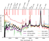 |
Fig. 1. Broadband spectrum of GN-9771 in comparison to other LRDs. We have highlighted the main emission lines on the top axis. We make a comparison with the PRISM spectrum of the other LRDs in our IFU program (Matthee et al. in prep.) and of A2744-45924 (Labbe et al. 2024), after normalizing their flux to match GN-9771 in the 5400–5700 Å band. The spectrum of GN-9771 is very similar to the spectrum of A2744-45924, with only a slightly weaker Balmer break in the case of GN-9771. |
We refer to Ishikawa et al. (in prep.) for a detailed description of the NIRSpec IFU data reduction. The data reduction was completed using the STScI JWST pipeline2 version 1.17.1 with Calibration Reference Data System version 12.0.9 (jwst_1299.pmap). The first stage, Detector1Pipeline, performs standard infrared detector reductions. We correct for the 1/f noise (Schlawin et al. 2020) on each detector by using a running mean algorithm. We also use snowblind3 to remove noise from snowball effects and cosmic rays. Then, these rate files are processed by Spec2Pipeline that produces calibrated spectra data, assigns the world coordinate system, and extracts the 2D spectra to build a 3D datacube using drizzle. Finally, we apply a sigma clip routine to mask pixels with extreme outliers and use the Photutils reproject method (Vayner et al. 2023) to align and combine the 8 dither exposures into a single datacube with a spatial resolution of 0.05″ per spaxel. Since no dedicated background exposures were taken, we perform aperture background subtraction from the datacubes. Both the PRISM and G395H/F290LP exposures showed non-uniform background. We detected a bright, narrow stripe that appears as an excess flux above the astrophysical background and stretches across the detector. To correct the background, we modeled the overall background (non-stripe regions) and the superimposed stripe artifact separately. Within these strips, the background was assumed to be uniform in each wavelength layer. We derived this uniform value from the running median value of empty-sky pixels, where we used a kernel of 10 wavelength layers. Empty-sky pixels were identified based on an agressive source detection in the white-light image of the PRISM and G395H data, respectively. Both components were subtracted to produce the final background-subtracted datacube. In late stages of finalizing the paper, we also reduced the data with msaexp (version 0.9.9; Brammer et al. in prep.). This reduction generally is hardly distinguishable from our standard reduction. However, the msaexp reduction yields slightly better performance in the bluest part of the G395H data, in particular because it slightly extends the wavelength coverage from 2.87 μm to 2.80 μm which the crucial coverage of Hγ and [O III] λ4364. We have verified the flux calibration of this added range thanks to the oerlap with the available PRISM spectrum.
We find that GN-9771 appears spatially unresolved across the full wavelength coverage of our PRISM data, which is consistent with the NIRCam imaging data (Matthee et al. 2024). We also do not identify any neighbouring galaxies within the IFU field of view. Our measurements are therefore based on a 1D spectrum that is optimally extracted based on the light profile in a collapsed Hα pseudo-narrowband image that we for simplicity derived by fitting a 2D Gaussian. Our results remain unchanged when extracting the spectrum over a simple compact circular aperture.
3. Results: The optical emission lines of GN-9711
In this section we provide an overview of the spectral features detected in our new deep data on GN-9771.
3.1. Balmer lines and [O III] emission
To place our spectrum in the rest-frame, we obtain the redshift of the [O III] doublet of GN-9771 from the continuum-subtracted spectrum. This redshift will serve as reference for the rest of the analysis done in this paper because the redshift is most well defined due to the narrowness of the lines. The details of the continuum fitting and background subtraction of the grating spectrum are detailed in Appendix A. We fit two Gaussians with a fixed ratio of 2.98, and convolving the model with a Gaussian line spread function, using the nominal resolution of the G395H grating4. We thus obtain a redshift of z = 5.53453 ± 0.00004, and a Gaussian width of FWHM 202 ± 5 km s−1. This narrow line width suggests a very low dynamical mass, similar to other LRDs with recent deep G395H observations (e.g., D’Eugenio et al. 2025b; D’Eugenio et al. 2025a; Wang et al. 2025a).
In Figs. 2 and 3 we show the high-quality Hα and Hβ spectra of GN-9771, respectively. The Hα spectrum confirms the absorption system seen in the NIRCam grism data (Matthee et al. 2024) and we now show that the absorption is also present in Hβ with a similar velociy offset. The total Hβ flux is ≈10.4 times fainter than the Hα flux which is a strong departure from the case B ratio of ≈2.86 (see Sect. 5.2 for a discussion). The emission lines have prominent non-Gaussian wings (see also Rusakov et al. 2025; de Graaff et al. 2025b), whereas the core of the lines (the central ±1000 km s−1) resemble P Cygni profiles.
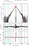 |
Fig. 2. Triangular P Cygni Hα spectrum of GN-9771. The continuum-subtracted Hα spectrum based on the G395H data is shown in black, whereas the red line shows the best-fit combined model (BIC = 932). Residuals to the model are shown in the middle panel. The fiducial fitting model is described in Sect. 3.1. We indicate the masked regions based on the locations of possible narrow [Fe II] emission in Véron-Cetty et al. (2004) (teal) and He Iλ6680 (purple). The [N II] component is not shown due to its relative flux being negligible. The bottom panel shows the Hα spectrum and best fit after subtracting the exponential component to highlight the P Cygni profile. |
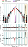 |
Fig. 3. Hβ spectrum of GN-9771. We used a similar model setup to that for Hα described in Fig. 2 (BIC = 74). The teal regions have been masked due to possible Fe II emission. The orange region indicates the masked [O III] wavelengths. The bottom panel shows the Hβ spectrum and best fit (red) after subtracting the exponential component to highlight the P Cygni profile. Figure B.1 shows a version of the same fit with the exponential scale fixed to that fitted for Hα. |
We fit the Hα and Hβ lines of GN-9771 to a model consisting of a narrow Gaussian emission, a Gaussian absorber, a broad exponential, and a host Gaussian component. We call this our fiducial model. These components are chosen arbitrarily to match the observed shape, and the individual physical interpretation of some of the components is not necessarily meaningful. The host component has width and redshift fixed to those of the [O III] lines, is included in the model to represent a hypothetical host galaxy contribution. The velocity offsets of all the components–except the host component–are allowed to vary within ±500 km s−1. For the fit, we mask the wavelengths potentially affected by [Fe II]. We define the [Fe II] masks using the lines seen in the N3 system of I Zw1 (Véron-Cetty et al. 2004). We also mask other detected lines such as He Iλ6680 and [O III] λλ4960, 5008. Since the preliminary continuum subtraction based on a power law might not be completely accurate, we also introduce a wavelength-constant continuum level in the line fit.
We note that the [Fe II] emission affects the flux of the exponential wings severely. The measured flux of [Fe II] is ≈7% of the total Hβ flux within ±3000 km s−1 of Hβ’s systemic velocity. This is only evident for this object due to the exceptionally high S/N of our spectrum. This component should be taken into account to investigate the differences in line profiles among different Balmer lines of other LRDs in future works.
We list the parameters of the best-fitting models to Hα and Hβ in Table 1. The velocity offset of the exponential component implies that the exponential component is either not symmetric around the systemic redshift, or that there is a general velocity shift to the region that produces the [O III] emission. The main narrow Hα emission component is significantly broader than the [O III] emission, while this is less conclusive for Hβ. We note that these components of our fiducial model are purely descriptive as they are meant to capture the general P Cygni shape of the line core. The specific physics involving resonant Balmer radiative transfer in Compton-thick media are complex and require more complex modeling (e.g., Shimoda & Laming 2019; Chang et al. 2025).
Table of best-fit parameters for Hα and Hβ.
The broad wings of the Hα line are very well described by a simple exponential up to at least ∼ ± 8000 km s−1. Our fiducial model with exponential wings (BIC = 932) works significantly better than replacing the exponential with a broad Lorentzian component (BIC = 1027, ΔBIC ≫ 10; see Fig. B.2). The best-fit exponential has a width of FWHMexp, Hα = 1549 ± 5 km s−1. For Hβ we obtain FWHMexp, Hβ = 2180 ± 490 km s−1. With this model, the best-fitting exponential wings of Hβ are wider than Hα, with a significance of ∼1.3σ. If electron scattering is the cause of the broad Balmer line wings (e.g., Rusakov et al. 2025), the FWHM of the exponentials is expected to be the same as long as the scattering of the different lines is produced in the same layers within the envelope. This is due to the cross-section of the scattering being wavelength independent in the Thomson regime (e.g., Juodžbalis et al. 2025; Brazzini et al. 2025; Chang et al. 2025). To test this, we both Hα and Hβ simultaneously, fixing the exponential width of both lines, and masking the central ±1000 km s−1. Fixing the exponential to the same value yields an exponential width of FWHM = 1613 ± 17 km s−1, and the best fit is not significantly worse (BIC = 258) than leaving the widths of each line free (BIC = 251).
To investigate the significance of the host Gaussian component, we repeat the fit to Hα and Hβ with our fiducial model, but removing this component. In the case of Hα, we obtain a best fit with BIC = 931 (ΔBIC ≈ 1; Fig. B.3), indicating that the host component has no statistical significance. In turn, for Hβ a better BIC = 67.6 (ΔBIC ≈ −6) is obtained. This result highlights the degeneracy of the model in the core of the line, as shown in Fig. B.4, our model with no host fits a narrow Gaussian component which could mimic a host Hα with a similar width to [O III].
3.2. Balmer break
The rest-frame UV and optical spectrum of GN-9771 shows the characteristic features of many LRDs (see Fig. 1): a Balmer break, broad Balmer lines and a relatively blue UV continuum. The prism spectrum also shows forbidden lines with high excitation energies such as [O III] λλ4960,5008, [O III] λ4364 (blended with Hγ), [Ne III] λ3869 and C III] λ1909. Similar to A2744-45924, the prism spectrum shows indications of strong Fe II emission, both in the UV and the optical (see below), and He I and [O I] emission. Notable as well are the absence of Lyα emission and the downturn in the far-UV λ < 2000 Å part of the spectrum, which is not seen in all LRDs.
The Balmer break is one of the key features in the spectra of LRDs (e.g., Setton et al. 2025a). We follow the parametrization of de Graaff et al. (2025b) and define it as fν, 4000 − 4100/fν, 3620 − 3720, where fν, 3620 − 3720 is the median flux density over the λ0 = 3620–3720 Å range. For GN-9771, the Balmer break strength is 2.5 ± 0.04, which is close to the maximum value of ≈3.0 that typical stellar populations can reach (Wang et al. 2024) and similar to other very red LRDs (A2744-45294 has a break strength of ≈3.4). It is not as extreme as the Balmer breaks of BB ≈ 7 measured in The Cliff (de Graaff et al. 2025b) or MoM-BH*-1 (Naidu et al. 2025).
3.3. A forest of [Fe II] emission, Hγ, and [O III] λ4634
Figure 4 shows our deep high-resolution grating spectrum zoomed in on the region around the Hβ and [O III] lines. Besides the very narrow [O III] emission discussed in Sect. 3.1 and the triangular Hβ profile, one can also notice a plethora of other fainter lines, most of which are emission lines from transitions from the singly ionized iron atom Fe II. The lines around wavelengths 5200 Å were initially identified as [Fe VII] λ5276 and [Fe VII] λ5159. However, our spectra do not show [Fe VII] λ6087 which is usually stronger (Petrushevska et al. 2023; Reefe et al. 2022), nor lines from any other high-excitation iron transitions. Upon inspecting the Fe II templates from I Zw1, we realized that most of the features were in fact unusually narrow [Fe II] emission lines.
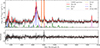 |
Fig. 4. [Fe II] forest detected in the G395H data over the ∼5000 Å region of GN-9771. We show the fitted [Fe II] spectrum as described in Sect. 3.3 (green), the He I lines (pink), Hγ (blue dot-dashed), the Hβ model (blue dashed), [O III] λλ4960, 5008 (orange dot-dashed), and [O IIIλ4364 (brown). The residuals of the fit as well as the observational uncertainties on the spectrum are shown in the bottom panel. |
Some of the most prominent [Fe II] emission lines lie very close to the rest-frame wavelength range of the broad Hβ and the [O III] doublet. In particular, the line profile of the broad wing of Hβ is contaminated by the relatively strong [Fe II] emission-line at 4815.9 Å. Before fitting the [Fe II] complex, we subtract the continuum as well as the model of Hβ and Hα, which were fit after masking all the potential [Fe II] lines as described in Sect. 3.1. The full model is convolved with the wavelength-dependent line-spread function, as defined by the nominal (wavelength-dependent) resolution of the G395H grating.
We obtain the list of forbidden (magnetic-dipole and electric-quadrupole) Fe II transitions in the range 4200–8000 Å from the NIST5 database (Kramida et al. 2024). Within a forbidden transition multiplet, the relative strength of the component n can be obtained as
 (1)
(1)
where Ji is the quantum number of the total angular momentum relative to the lower level, λ the emitted vacuum wavelength, and Aki the Einstein coefficient of the transition.
We fit our [Fe II] model to the rest-frame wavelength ranges 4200–6000 Å and 6350–8000 Å, which are the two wavelength intervals of our data separated by the detector gap. These first interval contains Hγ and Hβ, and the second interval includes Hα. The fitting model consists of a power-law continuum, the Hβ or Hα models as described above, a double Gaussian for the [O III] doublet with fixed flux ratio of 2.98, and the [Fe II] model. The former consists of Gaussians at the positions of every forbidden line in the NIST database, with a shared velocity width. We also allow for a small velocity offset as a free parameter, shared by all the [Fe II] lines. The Gaussian amplitudes within every multiplet are fixed using Eq. (1). In addition, we include in our model the He Iλ4472, λ4923, λ5017, and λ6680 as single Gaussians whose amplitudes and widths can vary freely, and the brighter He Iλ5876 and λ7067 as Lorentzians. In the case of these two lines, a Lorentzian gives a significantly better fit than a Gaussian, hinting a broad component. The He I spin-singlet lines at λ4923 and λ5017 Å are blended with Hβ and [O III], respectively. For this reason, we fixed the widths and velocity shifts of these two lines to the values fit for He Iλ58766. We also include Hγ and [O III] λ4364 components in the fit. The wavelengths of these two lines are very close to each other, which difficultates a precise assesment of both, moreover, strong [Fe II] emission is also expected in nearby wavelengths. For this reason, we model for Hγ consisting in a broad exponential with fixed velocity width to that fit to Hβ, a Gaussian absorber and a Gaussian host component with width tied to [O III] λλ4960, 5008.
We find that the [Fe II] lines are at a similar velocity as the [O III] λλ4960, 5008 velocity (offset by −43 ± 15 km s−1). The [Fe II] lines have an intermediate width of FWHM = 464 ± 61 km s−1, comparable to the width of the He I lines (within 1σ; see Table 2), significantly broader than the [O III] λλ4960,5008 doublet with FWHM = 156 ± 2 km s−1, but much narrower than the Balmer lines. The best-fitting model is shown in Figs. 4 and 5, and individual fluxes of the main (S/N > 1) [Fe II] lines are listed in Table 3.
List of relevant emission lines detected in the spectrum of GN-9771.
Main fitted forbidden [Fe II] line fluxes of multiplets.
The width of the best-fitting [O III] λ4364 Gaussian is 361 ± 74 km s−1, seemingly broader than the [O III] λλ4960, 5008 conterparts (with FWHM = 202 ± 5 km s−1), but with a significance of only 2σ. As shown in Fig. 5, [O III] λ4364 is potentially affected by a strong [Fe II] line, hindering a precise assesment. In fact, fixing the width of this Gaussian component to that of the λλ4960, 5008 doublet does not significantly worsen the fit (ΔBIC ≈ 4). We discuss the implications of the [O III] line width and the Hγ fluxes in Sect. 6.1.
3.4. UV Fe II: Absorption or emission
The emission spectrum of Fe II is complex, having hundreds of significant transitions and spanning from the UV to the optical and near infrared parts of the spectrum. We investigate the UV Fe II emission of GN-9771. Labbe et al. (2024) first reported prominent UV Fe II emission in their deep spectrum of the luminous LRD A2744-45924. However, the low resolution (R ∼ 100) of the PRISM spectrum hinders a assessment of the multiple Fe II transitions. GN-9771 presents a very similar UV Fe II bump, as shown in Fig. 1.
We fit the UV Fe II in the range 2000–3600 Å, using templates based on the galaxy I Zw1 (Vestergaard & Wilkes 2001; Salviander et al. 2007). In particular, we use the version of these templates from the code PyQSOFit (Guo et al. 2018), and convolving the model with an arbitrary Gaussian, to include the effects of the PRISM resolution and the intrinsic velocity dispersion of the lines. Due to the huge number of transitions, we do not attempt to fit a deconvolved width for UV Fe II. Following Labbe et al. (2024), we also include the Mg IIλ2799 and He IIλ3203 as Gaussians in the model.
The template fitting does not provide a satisfactory result (χν2 = 7.5; Fig. 6), particularly failing to reproduce the prominent bump at ∼2500 Å. The secondary bump at ∼2800 Å can only be matched by invoking a strong contribution from broad Mg II (see also Labbe et al. 2024; Tripodi et al. 2025). An alternative explanation would be that the ∼2500 Å bump could arise from absorption by the resonant Fe II multiplets UV1 and UV2+UV3, at ∼2600 and ∼2400 Å, respectively (see Sect. 6.1 for a detailed discussion).
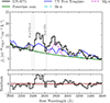 |
Fig. 6. Template fit to UV Fe II. We fit templates to the UV pseudo-continuum emission. The fitting is challenging due to the limited PRISM resolution in this wavelength range (R ∼ 50). The model includes the Mg II and Fe II lines, which are usually strong. The template fitting does not produce a satisfactory result (χν2 = 7.5), in particular for the ∼2500 Å bump. Absorption features from the resonant Fe II multiplets UV1 and UV2+UV3 are compatible with the observed shape of the continuum, which are also predicted by our Cloudy models (see Sect. 6.1 for a discussion). |
3.5. He I emission
As described in Sect. 3.3, we also identify six He I lines in our spectrum. Despite the high resolution of the G395H grating, some He I lines are blended with the broad tails of the Hβ and Hα lines. We first fit the He I line λ5876 – which has the highest S/N –, with a Lorentzian profile, which gives a slightly better χν2 than a Gaussian. Then, we fit the He Iλ5017 and λ4923 with Gaussians of the same FWHM as the Lorentzian He Iλ5876, and matching their velocity offset. The He Iλ4472 line is fitted independently with a Gaussian. The other high S/N line He Iλ7067 is also fitted to a Lorentzian, and the blended He Iλ6680 fit as a Gaussian, fixing the width and velocity offset in the same manner. Interestingly, He Iλ7067 is the strongest helium line that we cover, which is typically much weaker than He Iλ5877 in normal galaxies, and it is indicative of high gas density (see Sect. 5.3 for a discussion).
In Table 2 the fluxes of all the He I lines and others are listed. Both He Iλ5876 and λ7067 do not show a significant velocity shift with respect to [O III] λλ4960, 5008 (Δv = 2.4 ± 1.4 and 18 ± 8 km s−1, respectively). He Iλ4472 appears to be redshifted with respect to [O III] by Δv = 145 ± 40 km s−1, but the low S/N ≈ 2 of this line makes this measurement unreliable. We also detect remarkably strong He Iλ4923, λ5017 and λ6680 singlet lines. We note that there are [Fe II] multiplets contaminating these lines (especially the first two); however, our model disfavors them when the theoretical [Fe II] line ratios are taken into account.
4. Photoionization modeling
In this section we present Cloudy modeling to interpret the observed spectral features. We caution that these models are empirically motivated phenomenogical models whose main goal is to provide qualitative insights into the conditions and structure of the gas around LRDs.
4.1. Photoionized cloud model
We use Cloudy (version 23.01, last described in Chatzikos et al. 2023; Gunasekera et al. 2023) to simulate an intrinsic ionizing SED striking a cloud of very dense gas. The incident SED is that of a classical AGN with a blackbody temperature of 105 K, and power-law slopes αOX = −1.5, αUV = −0.5, and αX = −0.5 (Jin et al. 2012). We use the default atomic data for all the species, and solar relative abundances. These parameters are comparable to those used in similar setups to investigate the Balmer break of LRDs (Naidu et al. 2025; de Graaff et al. 2025b; Ji et al. 2025b). Similar models were explored thoroughly in the literature to investigate the Fe II emission of AGN (e.g., Baldwin et al. 1995, 2004; Wang et al. 2008; Ferland et al. 2009; Sameshima et al. 2011; Sarkar et al. 2021). We set the normalization of the incident SED varying the ionization parameter log10U from −4 to 0 with 1 dex steps. We simulate clouds with plane-parallel geometry, in a fairly broad range of hydrogen density nH = 106 to 1014 cm−3 and hydrogen column density NH = 1021 to 1026 cm−2, both with 1 dex steps. We also vary the turbulence velocity vturb = 10 to 510 km s−1 in steps of 100 km s−1 and the metallicity log10(Z/Z⊙) = − 2 to 1 with 1 dex steps. This produces a grid of 6480 models. We note that variations in the incident spectrum are to some extent degenerate with variations in the properties of the dense gas and therefore merit exploration on their own (e.g., Wang et al. 2025b). However, we have verified that our qualitative results on the density-temperature structure and origin of observed emission lines are not strongly impacted by our specific choice. As such variations are also degenerate with the possible contribution from the host galaxy, we defer the detailed investigation where the incident spectrum is also varied to the future when better high-resolution data is available in the UV and blue optical regime.
We fit the observed rest-frame optical spectrum with the Fe II emission predicted by the Cloudy models. The templates, convolved with a Gaussian–free width, velocity offset, and normalization–are combined with the same continuum and line components as in Sect. 3.3. The fit is performed on the relative Fe II fluxes rather than equivalent widths, focusing on the line flux ratios.
We perform a least-squares fit of each template of the grid to the rest-frame optical Fe II spectrum of GN-9771–no other measurements are included in this fit. We find that the best fit (χν2 = 1.49) is obtained for the model with log10U = −3, nH = 108 cm−3, NH = 1022 cm−2, vturb = 210 km s−1 and log10Z/Z⊙ = −2. In Fig. 7 we show the minimum χν2 across the grid for each point in the (nH, NH) plane for this photoionized cloud model. In general, this model reproduces relatively well the observed optical [Fe II] for densities of nH = 107 − 10, and slightly prefers a relatively low column density. Lower values of ionization parameter (i.e., log10U = −4) yield similarly good fits to the [Fe II] line ratios of GN-9771, but have more difficulties to reproduce the strong Balmer break at the same time. The metallicity parameter, in turn, has a minor role for line ratios, yielding similar results for all probed values (log10(Z/Z⊙) = − 2 to 0). The turbulence parameter vturb also has a minor effect on the optical [Fe II] ratios; however, a high vturb is preferred to obtain a smooth Balmer break (see also Ji et al. 2025b; Naidu et al. 2025).
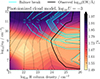 |
Fig. 7. Density and column density of the warm layer as preferred by the [Fe II] line-emission compared to that preferred by the Balmer break strength. The colored contours show the values of χν2 of our fit to the optical [Fe II] of GN-9771 to Cloudy photoionized cloud models with vturb = 210 km s−1 and Z/Z⊙ = 0.01. We also show the strength of the Balmer break for the grid of models as cyan contour lines, where we highlight the approximate Balmer break strength (≈2.5) of GN-9771 with a shaded region. The black line marks the contour of the models with matching [Fe II] EW to the observed in GN-9771, in the range 5100–5400 Å. Dashed lines indicate contours of ×2 difference in EW (increasing toward the right-hand side of the figure). |
In Fig. 7 we also show the Balmer break strength produced by the models in the grid. Only the models with nH ≈ 109 − 10 cm−3 and NH ≳ 1024 cm−2 can produce reasonable [Fe II] line ratios–taking into account the simplicity of the model–and simultaneously accomodate Balmer breaks that roughly match the one observed in GN-9771. In any case, this model is only able to reproduce the [Fe II] for nH < 1010 cm−3. We conclude that the photoionized cloud model prefers gas densities of nH = 109 − 10 cm−3 and high column densities NH > 1024 cm−2 to reproduce the observed [Fe II] ratios and Balmer break of GN-9771, as well as the EW of the [Fe II] lines. On the one hand, the EW of the [Fe II] emission increases for higher values of NH, highlighting the need of a thick layer of gas adding to the total [Fe II] emissivity. On the other hand, the EW also naturally increases for higher gas metallicity, hence there is a degeneracy between the two parameters. One caveat of the choice of a plane-parallel geometry is that this assumption is only valid in the case that the distance from the ionizing source to the inner face of the cloud is much larger than the cloud thickness. For our models, the inner radius is set by the ionization parameter, if one would assume a spherical geometry. For log10U = −3 and log10(nH/cm−2) = 9–10 the inner radius would be ≈1017–1018 cm, roughly more than two orders of magnitude larger than the implied cloud depth given by NH/nH.
4.2. Overall spectral shape
In photoionized cloud models (BH*), the Balmer break strength is explained as the absorption of the intrinsic (AGN-like) SED by the partially ionized gas. The strength of the break is thus directly suggestive of high gas column densities (e.g., Inayoshi & Maiolino 2025; Naidu et al. 2025). The Balmer break strength in this scenario also depends on the gas volumetric density and temperature (e.g., Liu et al. 2025) and the dense gas covering fraction.
In Fig. 8, we show the best-fitting BH* continuum to the PRISM spectrum of GN-9771, from a larger grid of models presented in Naidu et al. (2025), extended down to log10U = −4. This larger sample also explores variations in the input SED parameters, so we adopt it for fitting the continuum. A pre-selection was made to match the approximate Hα and Hβ EWs (EW(Hα) = 1500–2000 Å, EW(Hβ) = 100–200 Å) and Balmer break (0.5–5). The best-fitting model is selected by least-squares minimization matching the continuum to the GN-9771 prism data in the shaded gray wavelength intervals shown in Fig. 8, adding an arbitrary normalization. The best-fit model corresponds to an incident AGN SED with TBB = 5 × 10⁴ K, αOX = −1, αUV = −1, αX = −0.5, log10U = −3, nH = 1010.5 cm−3, NH = 1023.5 cm−2, vturb = 300 km s−1 and Z/Z⊙ = 0.01. The best-matched BH* model is convolved with the PRISM line-spread function. The BH* model is capable to reproduce the overall shape of the optical+UV continuum of GN-9771, including the shape of the Balmer break due to turbulent broadening of the Balmer series absorptions. The fact that the best-fit parameters are similar to those obtained in Sect. 4.1 suggests that a BH* model can simultaneously reproduce both the overall spectral shape and optical [Fe II] emission, although a more definitive assessment is left for future work. The lack of some emission lines, for example [O III] and [Ne III] λ3869, could be explained by an additional host galaxy component, due to their low critical densities (further discussed in Sect. 6.1).
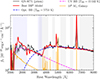 |
Fig. 8. Best-matching BH* model and blackbody fit to the optical spectrum. We matched the gray shaded wavelengths to the larger model grid presented in Naidu et al. (2025). We also show the blackbody that best fits the rest-frame optical (dashed blue) and UV (dashed purple), for which we obtain an effective temperature of TBB, opt = 5753 K (fit to wavelengths highlighted with a gray shade) and TBB, opt = 15 530 K (purple shade), respectively. For illustration, we also include the SED fit to the object ALT-31334 (z = 5.66; M* = 108 M⊙), a typical compact blue galaxy that could resemble a hypothetical host for GN-9771 (see Sect. 6.1). |
For reference, we also fit a Planck blackbody law to the optical and UV continua of GN-9771 (see, e.g., Zwick et al. 2025). The optical (3640–8000 Å) continuum is well fit by a blackbody with an effective temperature of TBB, opt = 5753 K, using the wavelength ranges marked as shaded gray areas in Fig. 8. Despite the good fit over a broad range of optical wavelengths, the spectrum of GN-9771 has a more abrupt drop-off than a blackbody toward the Balmer break (≈3700 Å), this suggests that a blackbody alone cannot reproduce the emission, but a Balmer break from neutral hydrogen absorption is also needed in this case. The measured blackbody temperature of the optical emission is in line with Liu et al. (2025), who suggested that the continuum emission of LRDs could be explained as a cool photosphere with T ≈ 5000 K. Our BH* models can reach similarly low temperatures at the edge of their envelopes (see Fig. 9). Some works have proposed that the UV emission of LRDs could arise from hotter accretion disk components (e.g., Inayoshi et al. 2025b; Zhang et al. 2025). We also fit another blackbody to the UV continuum (1000–3600 Å), with an effective temperature of T = 15 530 K. We note that our BH* models can mimic such blackbody-like continuum shape in the UV as the result of the absorption of the incident UV powerlaw by the neutral gas. However, we note that adding these two blackbodies would not reproduce the sharpness of the Balmer break, yielding a profile that is too smooth (e.g., Setton et al. 2025a; Wang et al. 2024; Ma et al. 2025b).
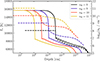 |
Fig. 9. Temperature-density structure of a suite of BH* models. We show the electron temperature (solid lines) and electron density (dashed lines) profiles for models corresponding to log10U = −3, vturb = 210 km s−1 and Z/Z⊙ = 0.01, for a wide range of hydrogen densities. All models are characterized by a hot (∼16 000 K; see Fig. D1 for the temperature with different choices of ionization parameter) and dense ionized region whose temperature and density abruptly drop at an ionization front, its radius dependent on density, and a thermalized outer layer of ∼6000–7500 K. |
The BH* model can reproduce the very high Hα/Hβ ratio, and also shows very weak Hγ emission. The [O III] lines are not well reproduced by our BH* model (λ4364 and λλ4960,5008), but these could be explained with contributions from a host galaxy (see Sect. 6.1).
5. Interpretation
An attractive feature of photoionized slab models (from now on, also referred to as Black Hole Star models; BH*; Naidu et al. 2025) is its capability to explain many of the most unusual spectral features of LRDs with the simple approach of a constant density gas illuminated by an incident ionizing SED. Therefore, we use this phenomenological model to interpret the origin of various observed spectral features in the spectrum of GN-9771. Table 4 summarizes the key points and challenges.
Summary of the observed features in the FRESCO-GN-9771 LRD and their interpretation in the context of the black hole star photoionization model.
5.1. Where the various spectral features originate
In photoionized cloud (BH*) models, due to the high densities considered, most UV ionizing radiation is deposited in a thin hot layer at the illuminated face of the cloud, generating an ionization front. The gas in the outer layers is then thermalized to temperatures of 6000–7500 K. In Fig. 9 we show the temperature and electron density dependence for BH* models with log10U = −3 and varying density (see also Fig. D1 for the dependence of these on the choice of log10U). The thermalized layer is partially ionized, that is, there is still a significant amount of free electrons (ne/nH ∼ 0.01–0.001). The size of this region depends mainly on the density and the ionization parameter, while its temperature is stable with the choice of different ionization parameters for the same density. The metallicity also plays a role in the total size of the thermalized region, as it regulates the temperature drop in the outer layers, and vturb has a negligible effect.
In Fig. 10 we show the outward emissivity of some optical emission lines for BH*-like models with nH = 1010 cm−3, for a total column density of NH = 1025 cm−2. The photon energy needed to ionize an iron atom to the Fe+ is 7.9 eV, and those are ionized further with photon energies exceeding 16.5 eV. For comparison, the ionization potential of neutral Hydrogen is 13.6 eV. The forbidden [Fe II] lines have relatively low critical densities of (ne ≈ 106 − 7 cm−3 at Te = 104 K, weakly dependent on temperature; Mendoza et al. 2023). [Fe II] is thus characteristic of partially ionized regions (e.g., Zhang et al. 2024). However, we note that in gas with high column density, significant line emission can still arise at electron densities well above the critical value, since the contributions from a large path length of emitting material along the line of sight add up. In our photoionized models, the optical [Fe II] emissivity is maximal for a gas temperature of ∼7500 K.
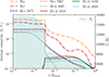 |
Fig. 10. Origins of the lines. The intrinsic emissivity of selected emission lines in the photoionized Cloudy model, for nH = 1010 cm−3, and NH = 1025 cm−2. Emissivities are expressed in arbitrary units of energy per unit time per unit volume. The ionization parameter is log10U = −3. The hydrogen Balmer and helium lines are intrinsically strong in the inner layers due to recombination emission, although the opacity of Hα and Hβ is high, which leads to scattering effects. [Fe II] is mostly emitted in a warm layer with Te = 6000–7500 K, which is shielded from the far-UV ionizing radiation. |
We conclude that the strong [Fe II] emission lines of GN-9771 arise from a warm (Te ≈ 7000 K) outer layer of dense (nH ≈ 109 − 10 cm−3) and partially ionized (ne ≈ 107 − 8.5 cm−3) gas with high column density (NH ≈ 1024 cm−2). This same warm layer is potentially the origin of other relevant spectral features such as the Balmer break, absorption, and the shape and relative intensities of the Balmer lines, as discussed in Sect. 5.2 below.
5.2. Insights from the Balmer lines
The maximum Hβ and Hα emissivities in our models are reached close to the illuminated face of the cloud (r/Rcloud ≲ 10−5), similar to the He I lines (Fig. 10). In this layer, the line emission is mainly driven by photoionzation and recombination radiation. However, due to the relatively small size of this layer, the contribution of this emissivity to the total can only be subdominant. The ratio of the observed Balmer lines Hα/Hβ = 10.4 ± 0.3 (9.0 ± 0.8 for the exponential wings only) and Hγ/Hβ = 0.14 ± 0.03 (0.13 ± 0.04) is far from the theoretical Case B recombination values of 2.86 and 0.47, respectively, for an optically thin, photoionized gas, or the value of Hα/Hβ = 3.1 that is often adopted for AGN narrow-line regions (Osterbrock & Ferland 2006). An explanation for the high ratio could be that there is a significant contribution from collisional excitation in addition to photoionization to the fluxes of the Balmer lines (e.g., Raga et al. 2015). Despite an ionized fraction of 0.99 in the hot layer, the neutral hydrogen density is still a few times 108 cm−3, making such collisional excitation scenario plausible. In the high density, optically thick limit, the relative populations of the n = 3 and n = 4 levels tend to obey the Boltzmann distribution, resulting in collisionally excited lines with an Hβ/Hα that declines exponentially with decreasing temperature. Following a similar analysis as presented in Nikopoulos et al. (2025), and using a standard Cardelli et al. (1989) dust attenuation law, we obtain E(B − V) = 1.15 ± 0.10 from the Hα/Hβ broad exponential component ratio, and E(B − V) = 2.6 ± 0.5 from Hγ/Hβ. Such values would imply an extreme dust obscuration (e.g., Woodrum et al. 2025). Moreover, the attenuation coefficients obtained from both Balmer ratios are in strong tension with each other, making it unlikely that dust attenuation is driving the observed Balmer decrements.
As the photons travel outward, the high column density of gas in the 2s state in the thermalized layer will cause resonant scattering, which impacts Hα and Hβ photons differently. Resonant scattering mainly impacts the core profile of the line, where absorption in the partially ionized layer (ne/nH ∼ 0.01) causes the blue-shifted absorption profile (Chang et al. 2025). In our Cloudy slab models, we find that the density of H atoms in the 2s state first increases sharply outward (by two orders of magnitude), peaking at the edge of the hot region, after which it remains relatively constant at a density of nH, 2s ∼ 103 cm−3 in the warm extended layer). In Fig. 11 we show the density of the fully ionized and three first levels of neutral hydrogen for a slab model with nH = 1010 cm−3 and NH = 1025 cm−2 and our fiducial AGN SED with log10U = −3. A column density of N(H I,2s) ≈ 1016 cm−2 is reached in this model–a similar configuration produces electron scattering dominated Hα and Hβ with P Cygni cores in Chang et al. (2025). The gas layer can also explain the broadening of the Balmer lines by electron scattering. The nominal Thomson optical depth in this layer is τe ∼ 0.01–0.1, slightly lower than what is predicted in Chang et al. (2025) for an observed FWHM ≈ 1500 km s−1 at ∼104 K, but resonant scattering can greatly increase the path length of Balmer photons, hence the effective Thomson opacity, making this hypothesis viable.
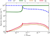 |
Fig. 11. Density of hydrogen species inside a photoionized slab. We show the volumetric density of fully ionized hydrogen (blue dashed) and first three levels (1s, 2s, 2p) of neutral hydrogen (solid lines) as a function of depth into the photoionized cloud of Fig. 10. Although most neutral hydrogen in the envelope is in the 1s state, there is a significant population (ne ≈ 103 cm−3) of electrons in the 2s state, which produces the Balmer break, and resonant scattering of Balmer lines (N(H I, 2s) ≈1016 cm−2). The high column density of free electrons in the same region could be responsible for electron scattering broadening of the Balmer lines. |
The high opacity of this envelope gas to the Balmer transitions is seen as the Balmer absorption present in both Hα and Hβ. In a gas that is optically thick to Balmer lines due to the metastable 2s state, higher Balmer transitions are efficiently converted into Hα, pushing the Hα/Hβ ratio to even higher values (Chang et al. 2025). This is an effect analogous to the Lyman Case B approximation (the so-called Balmer on-the-spot approximation; e.g., Osterbrock & Ferland 2006). A combination of this effect with the aforementioned collisional excitation effects of high column density gas are likely driving the steep Balmer decrement observed in GN-9771 and other LRDs in the literature.
One striking feature is the fact that the Balmer absorption appears to be relatively stronger in Hβ than in Hα, whereas it is theoretically expected to be the opposite. This has previously also been observed in other LRDs (e.g., D’Eugenio et al. 2025a). However, as discussed in Sect. 3.1, our fiducial model also admits an absorption component with a fixed τ(Hβ)/τ(Hα) = 0.137, albeit yielding a significantly worse BIC value (ΔBIC ≈ 16). Therefore, our fiducial model still predicts a tension with the theoretical optical depth ratio, although the tension can be alleviated when taking into account the degeneracies of the emission components in the line core. On the other hand, a tentative deviation of the theoretical τ(Hβ)/τ(Hα) = 0.137 could be explained by different Balmer lines being effectively emitted at slightly different depths into the cloud. We note that the optical depth to Balmer absorptions in a neutral dense gas is very high, facilitating this effect within not very large physical distances. This hypothesis could also explain the tentative difference in the exponential wing widths of Hα and Hβ (see Sect. 3.1), as both lines would potentially experience different electron column densities. Alternatively, this result could be attributed to differences in the absorption infilling, if relatively higher fraction of Hα emission is emitted at the edge of the cloud compared to Hβ (see Fig. 10). This could occur in the case that Hα and Hβ emission is driven by collisions in the edge of the warm layer, also evidenced by the lack of P Cygni emission in Hβ. The P Cygni components of Hα and Hβ (Fig. 2) interestingly have comparable line widths as the [Fe II] emission, suggesting that both the Balmer lines and [Fe II] could indeed partially originate from the warm layer. Alternatively, this component could originate from the resonantly scattered Hβ photons that branched to Hα. We emphasize that due to the strong degeneracies of our fiducial model used to fit Hα and Hβ, addressing the flux and spectral shape of this infilling component remains challenging (see Sect. 3.1). Generally, more tailored radiative transfer simulations (e.g., building upon the model presented in Chang et al. 2025), incorporating the effects of collisional excitation, are required to further study the exact conditions yielding the high Hα/Hβ ratios and explaining the detailed differences in the line-profiles.
Contrary to Hα and Hβ, the higher Balmer transition line Hγ seemingly contains an important contribution of a narrow component, compatible with the width of [O III] λλ4960, 5008. This result is in line with the interpretation that this narrow component is produced by a host galaxy. Under this assumption, the narrow components of all the Balmer lines would follow line ratios closer to the typical Case B ratios, assuming a low dust attenuation. Therefore, the narrow Hγ emerges, whilst in Hβ and Hα the respective narrow components are outshined by the broad, collisionally and/or scattering-dominated emission with higher relative intensities. In this scenario, the narrow Hγ component is a compelling tracer of the host of GN-9771, which we discuss in Sect. 6.1 in detail.
5.3. Insights from Helium emission lines
Unlike as is the case for the Balmer lines, the dense gas is optically thin to other lines, for example He I, He II, and [Fe II], making these promising probes of the internal dynamics and ionization conditions of LRD envelopes (e.g., Wang et al. 2025b), since they traverse it without being heavily affected by self-absorption (except perhaps by electron scattering). Although the HeI 4472, 5877, 7067 lines are much fainter than the Balmer lines and therefore detected only with modest signal to noise, they appear to show broad wings (Section 3.5, see Fig. 4). This is in line with our modeling that suggest they originate in the same gas as the Balmer photons. As the cross-section to Thomson scattering is independent of wavelength, this will yield similar broad wing, but they are not subject to resonant scattering such that the photons in the line-center escape through the warm layer more easily.
The He Iλ5876 line is a strong recombination line, often found in the spectra of Type 1 AGN with broad profiles (e.g., Vanden Berk et al. 2001; Kuhn et al. 2024). This line arises from de-excitation to the triplet level 23S of He from higher levels, along with other triplet lines (He Iλ4472, 7067). However, 23S is a metastable level, therefore in dense media it can be depopulated via collisions, in particular in absence of a strong ionization field (Mathis 1957; Benjamin et al. 2002). The observed ratios of the He I lines are therefore highly sensitive to density and temperature, in particular for high gas column densities (Almog & Netzer 1989).
Particularly interesting are the observed He I singlet lines, which intensity can be enhanced at very high densities if collisional effects are taken into account (e.g., Benjamin et al. 2002). These lines are rarely reported in spectra of most AGN populations (e.g., Véron et al. 2002). GN-9771 presents unusually high flux ratios of these lines when compared to the triplet line He Iλ5876: λ5876/λ5017 = 1.18 ± 0.4. Using the Python tool PYNEB (Luridiana et al. 2015), we estimate this ratio to be ∼6 in an optically thin, purely recombination driven scenario, for a broad range of gas density and temperatures. We note, however, that the He Iλ5017 line is potentially blended with [O III] and [Fe II], and the measured flux could be affected by these other lines. The He I singlet lines are also found to be strong in Type IIn supernovae, which are believed to have dense opaque gas envelopes (Groeningsson et al. 2007; Dessart et al. 2009) and therefore present similar configurations as those being considered for LRDs (e.g., Ji et al. 2025b; Naidu et al. 2025).
The strongest He I line in the observed wavelength range is λ7067. The ratio He Iλ5876/λ7067 = 0.85 is low in comparison with the typical values of 1.8–3 in star-forming galaxies at similar redshifts (e.g., Yanagisawa et al. 2024). The λ7067 line is strongly affected by complex radiative transfer and density effects, particularly for high densities, that could enhance its emission through pumping from the 23S level (e.g., Benjamin et al. 2002; Berg et al. 2025). Our photoionized cloud models fail to reproduce the high He Iλ5876/λ7067 ratio (see Fig. 10). More complex models that take these effects into account are needed in order to investigate He I ratios and intensities as density and temperature tracers, but generally the strengths of the singlets and the λ7067 line is a further proof that dense gas constitutes a central component of LRDs emission. The He IIλ4687 line is not detected in GN-9771; in line with the low emissivity predicted by our models (integrated emissivity ratio He IIλ4687/He Iλ5876 = 0.05; see Fig. 10).
6. Implications
6.1. Implications for the galaxies hosting LRDs
Given that GN-9771 appears to be a point-source at all observed wavelengths and that a significant fraction of the emission can be explained by the AGN emission in the context of the BH* model (Fig. 8), an important question to ask is where and what the host galaxy of GN-9771 is. Characterizing host galaxy is important to better understand the context of BH formation models and SMBH-galaxy co-evolution.
Here we attempt to quantify the fraction of the UV continuum that originates from the host galaxy. We assume that the key feature that traces the host galaxy emission is the [O III] emission due to its extremely narrow line width, even compared to AGN-associated lines as [Fe II]. The [O III] width implies a dynamical mass of log10(Mdyn/M⊙) = 9.6 ± 0.5, using the prescriptions from Bezanson et al. (2018). For typical galaxies, such dynamical mass would correspond to a stellar mass of log10(M*/M⊙)≈8, applying the scalings found in de Graaff et al. (2024), or log10(M*/M⊙)≈8.6 according to Saldana-Lopez et al. (2025). This is a very similar stellar mass was found by D’Eugenio et al. (2025a) for an LRD at a similar redshift and in line with clustering results (Matthee et al. 2025). Following this result, we can test the maximum contribution to the UV light from a blue host galaxy. We measure the UV absolute magnitude of GN-9771 to be MUV = −19.3 ± 0.4, based on the median flux density in the rest-frame 1400–1600 Å interval. For comparison, the median UV magnitude of 38 galaxies at 5 < z < 6, with masses 8 < log10(M*/M⊙) < 8.6 in the catalog of the ALT survey (Naidu et al. 2024) is MUV = −18.7 (ranging from −20.3 to −17.3). These results are therefore consistent with some contribution of a host galaxy to the UV spectrum of GN-9771, with the measured [O III], within the uncertainties given the broad scatter in Mdyn/M*. In Fig. 8 we include the SED fit by prospector to the object ALT-31334 (z = 5.66) as a typical example: a galaxy with log10(M*/M⊙) = 8.0 and MUV = −18.7, as expected for the host galaxy of GN-9771. It has a typical [O III] equivalent width of ≈700 Å; for comparison, the[O III] λλ4960, 5008 EW of GN-9771 is 370 ± 14 Å (see, e.g., Matthee et al. 2023; Endsley et al. 2024). This example illustrates how a typical low-mass galaxy can explain the observed narrow [O III], a minor fraction of the narrow Balmer emission-lines and with a minor contribution to the overall UV-optical spectrum of the LRD, which is only dominant at λ0 < 1500 Å.
A surprising aspect of GN-9771’s UV spectrum is its noteworthy similarity with the luminous LRD A2744-45924, with also a very similar MUV = −19.2. In particular, they share the same shape around 2400–3000 Å, which we argued in Sect. 3.4 it can be partly shaped by low-ionization Fe II absorption. Identical UV features are also present in other luminous LRDs (e.g., Tripodi et al. 2025; D’Eugenio et al. 2025c). Such features are characteristic of low-ionization absorption systems, frequently observed in FeLoBAL quasars (e.g., Zhang et al. 2022). However, under the assumption that the 2500 Å bump is a result of resonant UV Fe II multiplet absorptions, the rest of the UV features are hard to explain. It is possible that this part of the SED of GN-9771 is shaped by multiple overlapping absorption troughs, which is not unusual in FeLoBAL systems, as their shapes is very diverse (e.g., Hall et al. 2002). Notably some FeLoBALs show similar Balmer absorptions as reported in LRDs (Leighly et al. 2025). The strong similarity of the UV spectrum of GN-9771 and other luminous LRDs (Tripodi et al. 2025; Labbe et al. 2024; D’Eugenio et al. 2025c) suggests that these objects must have significant contribution from AGN to their UV light, as the observed features are hard to explain with a dominating star-forming host. This result is in line with the spatially resolved offset found in Torralba et al. (2026) between the compact Hα emission and the far-UV and Lyα of A2744-45924, the latter associated with the host galaxy. Deeper and high-resolution data would be needed to investigate the UV features of GN-9771 in detail, since the low PRISM resolution difficultates this task.
Additionally, the narrow components of the Balmer lines (see Sect. 3.1) also provide insights into the properties of an hypothetical host galaxy. The modelling of the Hγ line is challenging due to blending with [O III] λ4364 and multiple strong [Fe II] lines in the vicinity. Assuming a saturated Hγ absorption by the dense gas–that is, the absorption only affects the broad component of this line, and not the continuum–we obtain a narrow Hγ flux of 0.6 × 10⁻¹⁸ erg s−1. This flux can be regarded as a lower limit in the case that the Hγ absorption would significantly affect the continuum. Assuming Case B ratios, and disregarding dust attenuation in the host galaxy, this flux would correspond to a star formation rate of ∼5 M⊙ yr−1, using the SFR–Hα calibration from Kramarenko et al. (2026). Such SFR typically corresponds to star-forming galaxies at z ≈ 5 with log10(M*/M⊙)≈7.7–9.37 (e.g., Di Cesare et al. 2026), consistent with our estimate based on the dynamical mass. Still following the assumption of narrow Case B ratios, we obtain [O III]λ 5008/HβNarrow ≈ 5, which implies a gas-phase metallicity of 12 + log10(O/H) ∼ 7.4, slightly toward the low end of the mass-metallicity relation, but within the scatter (e.g., Chakraborty et al. 2025).
6.2. The nature of LRDs
In Sect. 5.2 we have presented multiple insights into the Balmer lines in the context of a dense gas envelope, summarized in Table 4. The exponential wings in the Balmer lines indicate a significant contribution to line broadening beyond gas dynamics (e.g., Naidu et al. 2025; Rusakov et al. 2025; Chang et al. 2025), unlike what is typically assumed for the quasar BLR. The P Cygni shape of the Hα and Hβ line cores result as a consequence of high opacity and resonant scattering in the warm envelope (e.g., Chang et al. 2025). Therefore, the shape of the P Cygni responds to the gas dynamics of the edge of the cloud, which in the case of GN-9771 is outflowing but could in other cases be inflowing (such as A2744-45924; Labbe et al. 2024). These results imply that the mechanisms governing the shape of Hα and Hβ–both in the line core and the broad wings–are very different from typical BLR conditions, as discussed in detail in Sect. 5.2. Due to the multiple differences in the Balmer lines, the standard scaling relations used to infer black hole masses and bolometric luminosities in quasars should, in general, not be applicable to LRDs.
The optical spectrum of GN-9771 does not show strong high-ionization lines, such as He IIλ4687, suggesting a cut-off in the incident spectrum (just) below ≈50 eV (e.g., Wang et al. 2025b). It also does not show lines with a low critical density, such as [N II] or [S II]. However, the spectrum does show [O III] λ4364 line. GN-9771 neither shows high-ionization lines in the UV (e.g., C IVλ1549, C IIIλ1909, Mg IIλ2799, typically strong in Type I & II AGN). In turn, collisional excitation seems to be an important mechanism for at least some of the optical lines, like the Balmer lines and [Fe II] (see, e.g., Kwan & Krolik 1981; Shields et al. 2010; Sameshima et al. 2011). Moreover, the high Hα/Hβ ratio may suggest a very significant contribution of collisional excitation processes to these lines (see Sect. 5.2 for a detailed discussion). An alternative explanation for the Balmer decrement would be very high dust attenuation, but this is at odds with, for example, the relatively blue optical colors. We note that broadband LRD spectra show significant variation (Fig. 1), especially in their UV spectrum. Whether such variations could be attributed to variations in host galaxy emission or in AGN conditions will be explored in a future work.
Using standard local virial calibrations, Matthee et al. (2024) obtained a BH mass of MBH = 108.55 M⊙ for GN-9771 (Greene & Ho 2005), fitting a broad Gaussian for a broad-line region. We estimate the bolometric luminosity of GN-9771 by integrating the best-fitting Cloudy slab model for λ > 912 Å (motivated by Greene et al. 2025), obtaining Lbol = 1044.95 erg s−1. This bolometric luminosity would imply a very low Eddington ratio of Lbol/LEdd = 0.02. This low value is in contrast with the super-Eddington scenarios recently proposed to explain many features of LRDs such as low continuum variability (e.g., Secunda et al. 2025; Furtak et al. 2025) or the lack of X-ray detections (e.g., Inayoshi et al. 2025a; Madau 2025; Madau & Haardt 2024, but see also Sacchi & Bogdán 2025).
Recent works have proposed models that describe many observed features of LRDs as photospheric emission from BH envelopes (Kido et al. 2025; Begelman & Dexter 2026; Zwick et al. 2025; Liu et al. 2025, e.g.,). In particular, Begelman & Dexter (2026) proposed a late-quasi-star scenario that describes many observed features of LRDs. The osberved properties of GN-9771 are very compatible with this scheme, which outlines a BH of mass MBH ∼ 106 M⊙ accreting at super-Eddington rates, yielding a luminosity of ∼1044 − 45 erg s−1, with optical color temperatures of ∼6000–7000 K (similar to the temperature of our modeled [Fe II] emitting envelope). Similarly, Liu et al. (2025), using semi-analytical atmosphere models, found that a super-Eddington system could yield an envelope with effective temperatures of 4000–6000 K that effectively reproduce the Balmer break and red optical colors of LRD, favoring models with high (super-)Eddington accretion rates. If Eddington-luminosity rate is assumed (fEdd ≡ Lbol/LEdd = 1), our measured Lbol would imply MBH ≈ 106.85 M⊙, which would correspond to an upper limit if super-Eddington accretion is invoked (see also Kokorev et al. 2023; Wang et al. 2025a). In combination with our stellar mass estimate (using the more conservative calibration of de Graaff et al. 2024), this result yields MBH/M* ≈ 0.1. If a higher fEdd = 10 is assumed, consistent with the value of Ṁ/ṀEdd = 102 favored by the models of Liu et al. 2025 (see Inayoshi et al. 2020), we obtain a BH mass of MBH ∼ 105.85 M⊙, yielding MBH/M* ≈ 0.01, greatly alleviating the tension with the local relation (Reines & Volonteri 2015). In Fig. 12 we show our different mass estimates in comparison with the observed local relation and simulated galaxies in the Illustris-TNG (Weinberger et al. 2017; Pillepich et al. 2018) and EAGLE (Schaye et al. 2015; Crain et al. 2015) simulations at z ≈ 5. These simulations have been calibrated to match the BH to stellar mass ratio in massive galaxies at z ∼ 0, but have not been tested in the early Universe. In the standard EAGLE and Illustris-TNG simulations, we notice that SMBHs in galaxies with masses ∼108 M⊙ are almost exclusively at the seed mass, i.e., there is no gas fueling SMBH growth yet, clearly at odds with observations of AGN in such low-mass galaxies, regardless of what the SMBH masses are. Interestingly, the EAGLE version without stellar feedback (ONLYAGN) enables SMBH accretion in lower mass galaxies, with some of the extremes having SMBHs with masses a few times 106 M⊙. This indicates that simulations of early galaxies with higher resolution that enables more efficient cooling of the ISM and SMBH growth (e.g., Chaikin et al. 2025) may contain galaxies hosting LRD phenomena.
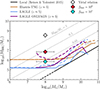 |
Fig. 12. BH vs. Stellar mass relation for GN-9771. We show estimations of MBH/M* for GN-9771 based on a stellar mass inferred from the dynamical mass suggested by the width of [O III], and MBH estimated using a standard virial relation (empty square; Matthee et al. 2024), and assuming an Eddington luminosity ratio of fEdd = 1 (red square), and fEdd = 10 (cyan square). We make a comparison with the local relation (Reines & Volonteri 2015) and the Illustris-TNG (Weinberger et al. 2017; Pillepich et al. 2018) and EAGLE (Schaye et al. 2015; Crain et al. 2015) simulations at z ≈ 5. We highlight the median trend with a solid (dashed) line and the extrema (95th percentiles) of the distributions in each simulation. |
6.3. Comparison to [Fe II] in other LRDs
Thanks to our new deep spectrum of GN-9771, we identify numerous previously poorly studied features of LRDs. Many of these emission-lines have been historically studied in the context of AGN, although their signatures differ in details. For example, while broad Fe II emission is commonly studied in quasar spectra, the relatively narrow forbidden [Fe II] emission is rarely seen in quasars. One notable exception is the quasar SDSS J1028+4500 at z = 0.58 (Wang et al. 2008). The spectrum of this object shows a very similar [Fe II] complex to that of GN-9771. Remarkably, it also shows significant Hβ and He I absorption, which is very rare among quasars. As we discussed in Sect. 5.1, the narrow [Fe II] lines are likely emitted in an intermediate-density warm gas with a high column density (NH ≳ 1024 cm−2). This same gas is arguably also responsible for the Balmer absorption seen in both Wang et al. (2008) and GN-9771–and, by extension, in other LRDs. Recently, [Fe II] has been clearly detected in a local (z = 0.1) LRD (Lin et al. 2025a; Ji et al. 2025a), the z = 2.3 Rosetta Stone (Ji et al. 2025a, see also Juodžbalis et al. 2024), and the LRD at z = 6.7 RUBIES-EGS-49140 (Lambrides et al. 2025; D’Eugenio et al. 2025c). The question remains if [Fe II] can be ubiquitously detected in LRDs with sufficiently deep data.
In order to investigate the prevalence of narrow [Fe II] emission in high-redshift LRDs, we stack publicly available medium- and high-resolution grating spectra of a sample of 13 LRDs at z = 4.13 − 6.98, covering Hβ and Hα to attempt detecting the [Fe II] lines also observed in GN-9771. In Fig. 13 we compare the grating spectrum of GN-9771 and the fit [Fe II] to a stacked sample of four objects in our NIRSpec IFU program (excluding GN-9771 itself; see Sect. 2)8 plus nine medium-resolution spectra of LRDs from the JADES (Eisenstein et al. 2023) and RUBIES (de Graaff et al. 2025a) surveys, publicly available in the Dawn JWST Archive9. For stacking, the high-resolution G395H spectra were degraded to match the resolution of the M grating (R ∼ 1000). We align each spectrum to a common rest-frame wavelength grid and normalize each spectrum to the average continuum flux density over 5300–5500 Å before we obtain a median stack. In the stacked spectrum, the most prominent [Fe II] features are indeed detected (λ4816, 5160, and 5275) with line ratios comparable to those seen in GN-9771.
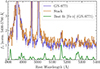 |
Fig. 13. Comparable [Fe II] emission in a stack of LRDs. We compare the [Fe II] optical spectrum of GN-9771 with a stack of 13 medium-resolution grating spectra of LRDs. The spectrum of GN-9771 is degraded to the medium resolution of the NIRSpec M-gratings for this comparison. The most luminous [Fe II] lines are detected in the stack, suggesting that these are common among LRDs, although their weak intrinsic fluxes challenge their detection. |
The variation among the strength of the optical [Fe II] emission, and the relation with other LRD properties (e.g., strength of the Balmer break, emission line properties etc.) should be tested with very deep grating spectroscopy in the future, due to the low intrinsic EW of [Fe II]. Assessing the prevalence of [Fe II] emission in LRDs will determine how our results apply to such broad population.
7. Summary
In this work, we employed JWST/NIRSpec IFU PRISM and high-resolution G395H data to investigate the properties of the luminous LRD FRESCO-GN-9771 at z = 5.535, and interpret them in the context of dense-gas envelope models (BH* models). In Table 4 we outline our interpretation of multiple common LRD spectral features in the context of BH* models. Below we summarize our main findings in this paper.
-
GN-9771’s Hα and Hβ emission line profiles are well described by a model consisting of broad exponential wings up to at least ± ∼ 7000 km s−1, and a P Cygni profile in the line cores (± ∼ 1000 km s−1). The exponential wings are in line with broadening by Thomson scattering, while the P Cygni cores may originate in a dense gas layer with high opacity to Balmer transitions. A broad Hγ is also detected, albeit with a lower S/N (Sect. 3.1, Figs. 2 and 3).
-
We detected a forest of multiple [Fe II] transitions in the rest-optical spectrum of GN-9771. These transitions are fit with fixed theoretical ratios. Their relative strength is high ([Fe II]/Hβ ≈ 0.13 in the range 5100–5400 Å), and they substantially contaminate the Hβ line profile, implicating that Fe II should be taken into account for the line fitting of this line (Sect. 3.3).
-
We measured a low He Iλ5876/λ7067 ∼ 0.81 ratio, which is another indicator of high-density gas, and suggests that complex radiative transfer effects play a crucial role in the emission of these lines. We also detected the typically faint singlet lines He Iλ5017 and λ6680. (Sects. 3.5 and 5.3).
-
We tested photoionization models computed with Cloudy, to investigate the origin of GN-9771’s emission lines. A BH*-like setup yields a best fit to the [Fe II] ratios for a gas density of nH = 109 − 10 cm−3 and column densities NH > 1024 cm−2, while still producing a Balmer break with a strength that is similar to what is observed. The [Fe II] emission is generated in a warm Te ≈ 6000–7500 K outer layer, shielded from strong ionizing radiation (Sect. 4).
-
The warm outer layer predicted by Cloudy models not only explains the [Fe II] emission, but is also the origin of the strong Balmer break and Balmer P Cygni profiles due to absorption by dense neutral hydrogen gas with a significant column density where the n = 2 state is significantly populated (N(H I,2s) ≈ 1016 cm−2). Additionally, the unusually high Hα/Hβ = 10.4 ± 3 and Hβ/Hγ = 7.1 ± 1.5 ratios are indicative that collisional effects and resonant scattering are significantly affecting the Balmer line emission. These processes happen in the warm, and partially ionized layer, which contains mostly neutral hydrogen, but also a fairly high electron density (ne/nH ∼ 0.01; Figs. 9, 10, and 11).
-
In addition to a similar broad wing, the Hγ profile shows a narrow component that is virtually unseen in Hα or Hβ. We associate this narrow emission with the host galaxy, and argue that this component is subdominant in the other two Balmer lines due to outshining by the broader emission, dominated by collisional processes and resonant scattering with flux ratios that strongly deviate from Case B. Meanwhile, the narrow component of all the Balmer lines should have ratios more similar to the expected in Case B recombination and trace host galaxy light (Sect. 6.1).
-
The narrow [O III] and Hγ emission suggest a host galaxy stellar mass of ∼108 M⊙ and a star formation rate of ∼5 M⊙ yr−1. On the other hand, the bolometric luminosity of GN-9771, log10(Lbol/erg s−1) ≈ 44.95, suggests a black hole mass of MBH ≈ 106.85 M⊙ assuming an Eddington-luminosity ratio of Lbol/LEdd = 1. This is roughly two orders of magnitude lower than local virial calibrations suggest. If higher Eddington ratios are assumed, the MBH/M* tension with the local relation and simulations is greatly alleviated (e.g., Lbol/LEdd = 10 would imply MBH/M* ≈ 0.01; Sects. 6.1 and 6.2).
These results show that LRDs are composite sources of a low-mass star-forming host galaxy, with a central AGN source that dominates the optical and even a significant fraction of the UV light (especially beyond λ0 > 1500 Å). The AGN is embedded in dense yet metal-enriched gas that is primarily found in a thermalized layer with a temperature of ∼7000 K. The emerging opacity to Balmer photons explains the strong and smooth Balmer break in the AGN spectrum, whereas collisional excitation and scattering processes in the warm layer explain the Balmer emission lines and their line profiles. Whereas scattering processes lead to non-dynamical broadening of the Balmer lines, the sheer luminosity (∼1045 erg s−1) and high gas densities remain the strongest evidence that an AGN is ultimately powering the emission. Nevertheless, many questions remain regarding the origin of the circumnuclear gas and the stability of the envelopes. Given that virial BH mass tracers may have become unreliable, perhaps we can only approximate black hole masses assuming Eddington accretion, although we remain unsure whether these results are applicable to the whole population of LRDs. These and other questions will occupy our focus for years to come.
Acknowledgments
We thank the scientific referee for useful and constructive comments. We thank Ylva Götberg and Zoltan Haiman for insightful discussions about the physics of gaseous envelopes and accretion into black holes. Funded by the European Union (ERC, AGENTS, 101076224). Views and opinions expressed are however those of the author(s) only and do not necessarily reflect those of the European Union or the European Research Council. Neither the European Union nor the granting authority can be held responsible for them. This work is based in part on observations made with the NASA/ESA/CSA James Webb Space Telescope. The data were obtained from the Mikulski Archive for Space Telescopes at the Space Telescope Science Institute, which is operated by the Association of Universities for Research in Astronomy, Inc., under NASA contract NAS 5-03127 for JWST. These observations are associated with program #5664. This work has received funding from the Swiss State Secretariat for Education, Research and Innovation (SERI) under contract number MB22.00072, as well as from the Swiss National Science Foundation (SNSF) through project grant 200020_207349.
References
- Akins, H. B., Casey, C. M., Lambrides, E., et al. 2025, ApJ, 991, 37 [Google Scholar]
- Aliste Castillo, R. L. S. E., Lee, Y.-H., Kokusho, T., et al. 2025, AJ, 169, 227 [Google Scholar]
- Almog, Y., & Netzer, H. 1989, MNRAS, 238, 57 [Google Scholar]
- Ananna, T. T., Bogdán, Á., Kovács, O. E., Natarajan, P., & Hickox, R. C. 2024, ApJ, 969, L18 [NASA ADS] [CrossRef] [Google Scholar]
- Arias, M. L., Zorec, J., Cidale, L., et al. 2006, A&A, 460, 821 [NASA ADS] [CrossRef] [EDP Sciences] [Google Scholar]
- Baggen, J. F. W., van Dokkum, P., Brammer, G., et al. 2024, ApJ, 977, L13 [NASA ADS] [CrossRef] [Google Scholar]
- Baldwin, J., Ferland, G., Korista, K., & Verner, D. 1995, ApJ, 455, L119 [NASA ADS] [Google Scholar]
- Baldwin, J. A., Ferland, G. J., Korista, K. T., Hamann, F., & LaCluyzé, A. 2004, ApJ, 615, 610 [NASA ADS] [CrossRef] [Google Scholar]
- Barro, G., Perez-Gonzalez, P. G., Kocevski, D. D., et al. 2024, arXiv e-prints [arXiv:2412.01887] [Google Scholar]
- Begelman, M. C., & Dexter, J. 2026, ApJ, 996, 48 [Google Scholar]
- Benjamin, R. A., Skillman, E. D., & Smits, D. P. 2002, ApJ, 569, 288 [Google Scholar]
- Berg, D. A., Sanders, R. L., Shapley, A. E., et al. 2025, arXiv e-prints [arXiv:2507.17057] [Google Scholar]
- Bezanson, R., van der Wel, A., Straatman, C., et al. 2018, ApJ, 868, L36 [NASA ADS] [CrossRef] [Google Scholar]
- Brazzini, M., D’Eugenio, F., Maiolino, R., et al. 2025, MNRAS, 544, L167 [Google Scholar]
- Cardelli, J. A., Clayton, G. C., & Mathis, J. S. 1989, ApJ, 345, 245 [Google Scholar]
- Carranza-Escudero, M., Conselice, C. J., Adams, N., et al. 2025, ApJ, 989, L50 [Google Scholar]
- Chaikin, E., Schaye, J., Schaller, M., et al. 2025, arXiv e-prints [arXiv:2509.07960] [Google Scholar]
- Chakraborty, P., Sarkar, A., Smith, R., et al. 2025, ApJ, 985, 24 [Google Scholar]
- Chang, S. J., Gronke, M., Matthee, J., & Mason, C. 2025, MNRAS, 545, staf2131 [Google Scholar]
- Chatzikos, M., Bianchi, S., Camilloni, F., et al. 2023, Rev. Mex. Astron. Astrofis., 59, 327 [Google Scholar]
- Chen, C.-H., Ho, L. C., Li, R., & Inayoshi, K. 2025, ApJ, 989, L12 [Google Scholar]
- Crain, R. A., Schaye, J., Bower, R. G., et al. 2015, MNRAS, 450, 1937 [NASA ADS] [CrossRef] [Google Scholar]
- de Graaff, A., Rix, H.-W., Carniani, S., et al. 2024, A&A, 684, A87 [NASA ADS] [CrossRef] [EDP Sciences] [Google Scholar]
- de Graaff, A., Brammer, G., Weibel, A., et al. 2025a, A&A, 697, A189 [NASA ADS] [CrossRef] [EDP Sciences] [Google Scholar]
- de Graaff, A., Rix, H.-W., Naidu, R. P., et al. 2025b, A&A, 701, A168 [NASA ADS] [CrossRef] [EDP Sciences] [Google Scholar]
- Dessart, L., Hillier, D. J., Gezari, S., Basa, S., & Matheson, T. 2009, MNRAS, 394, 21 [NASA ADS] [CrossRef] [Google Scholar]
- D’Eugenio, F., Juodžbalis, I., Ji, X., et al. 2025a, arXiv e-prints [arXiv:2506.14870] [Google Scholar]
- D’Eugenio, F., Maiolino, R., Perna, M., et al. 2025b, arXiv e-prints [arXiv:2503.11752] [Google Scholar]
- D’Eugenio, F., Nelson, E., Ji, X., et al. 2025c, arXiv e-prints [arXiv:2510.00101] [Google Scholar]
- Di Cesare, C., Matthee, J., Naidu, R. P., et al. 2026, A&A, in press, https://doi.org/10.1051/0004-6361/202557790 [Google Scholar]
- Eisenstein, D. J., Willott, C., Alberts, S., et al. 2023, arXiv e-prints [arXiv:2306.02465] [Google Scholar]
- Endsley, R., Stark, D. P., Whitler, L., et al. 2024, MNRAS, 533, 1111 [NASA ADS] [CrossRef] [Google Scholar]
- Ferland, G. J., Hu, C., Wang, J.-M., et al. 2009, ApJ, 707, L82 [Google Scholar]
- Furtak, L. J., Secunda, A. R., Greene, J. E., et al. 2025, A&A, 698, A227 [NASA ADS] [CrossRef] [EDP Sciences] [Google Scholar]
- Gaskell, M., Thakur, N., Tian, B., & Saravanan, A. 2022, Astron. Nachr., 343, e210112 [NASA ADS] [CrossRef] [Google Scholar]
- Gloudemans, A. J., Duncan, K. J., Eilers, A.-C., et al. 2025, ApJ, 986, 130 [Google Scholar]
- Greene, J. E., & Ho, L. C. 2005, ApJ, 630, 122 [NASA ADS] [CrossRef] [Google Scholar]
- Greene, J. E., Labbe, I., Goulding, A. D., et al. 2024, ApJ, 964, 39 [CrossRef] [Google Scholar]
- Greene, J. E., Setton, D. J., Furtak, L. J., et al. 2025, arXiv e-prints [arXiv:2509.05434] [Google Scholar]
- Groeningsson, P., Fransson, C., Lundqvist, P., et al. 2007, arXiv e-prints [arXiv:astro-ph/0703788] [Google Scholar]
- Gunasekera, C. M., van Hoof, P. A. M., Chatzikos, M., & Ferland, G. J. 2023, Res. Notes Am. Astron. Soc., 7, 246 [Google Scholar]
- Guo, H., Shen, Y., & Wang, S. 2018, PyQSOFit: Python code to fit the spectrum of quasars, Astrophysics Source Code Library [record ascl:1809.008] [Google Scholar]
- Hall, P. B., Anderson, S. F., Strauss, M. A., et al. 2002, ApJS, 141, 267 [NASA ADS] [CrossRef] [Google Scholar]
- Harikane, Y., Zhang, Y., Nakajima, K., et al. 2023, ApJ, 959, 39 [NASA ADS] [CrossRef] [Google Scholar]
- Hillier, D. J., Davidson, K., Ishibashi, K., & Gull, T. 2001, ApJ, 553, 837 [NASA ADS] [CrossRef] [Google Scholar]
- Inayoshi, K. 2025, ApJ, 988, L22 [Google Scholar]
- Inayoshi, K., & Maiolino, R. 2025, ApJ, 980, L27 [Google Scholar]
- Inayoshi, K., Visbal, E., & Haiman, Z. 2020, ARA&A, 58, 27 [NASA ADS] [CrossRef] [Google Scholar]
- Inayoshi, K., Kimura, S. S., & Noda, H. 2025a, PASJ, 77, 811 [Google Scholar]
- Inayoshi, K., Shangguan, J., Chen, X., Ho, L. C., & Haiman, Z. 2025b, arXiv e-prints [arXiv:2505.05322] [Google Scholar]
- Ji, X., D’Eugenio, F., Juodžbalis, I., et al. 2025a, arXiv e-prints [arXiv:2507.23774] [Google Scholar]
- Ji, X., Maiolino, R., Übler, H., et al. 2025b, MNRAS, 544, 3900 [Google Scholar]
- Jin, C., Ward, M., & Done, C. 2012, MNRAS, 425, 907 [NASA ADS] [CrossRef] [Google Scholar]
- Juodžbalis, I., Ji, X., Maiolino, R., et al. 2024, MNRAS, 535, 853 [CrossRef] [Google Scholar]
- Juodžbalis, I., Maiolino, R., Baker, W. M., et al. 2025, arXiv e-prints [arXiv:2504.03551] [Google Scholar]
- Kido, D., Ioka, K., Hotokezaka, K., Inayoshi, K., & Irwin, C. M. 2025, MNRAS, 544, 3407 [Google Scholar]
- Kocevski, D. D., Onoue, M., Inayoshi, K., et al. 2023, ApJ, 954, L4 [NASA ADS] [CrossRef] [Google Scholar]
- Kocevski, D. D., Finkelstein, S. L., Barro, G., et al. 2025, ApJ, 986, 126 [Google Scholar]
- Kokorev, V., Fujimoto, S., Labbe, I., et al. 2023, ApJ, 957, L7 [NASA ADS] [CrossRef] [Google Scholar]
- Kokorev, V., Caputi, K. I., Greene, J. E., et al. 2024, ApJ, 968, 38 [NASA ADS] [CrossRef] [Google Scholar]
- Koo, B. C. 2014, in Supernova Environmental Impacts, eds. A. Ray, & R. A. McCray, IAU Symp., 296, 214 [Google Scholar]
- Kramarenko, I. G., Rosdahl, J., Blaizot, J., et al. 2026, A&A, in press, https://doi.org/10.1051/0004-6361/202557114 [Google Scholar]
- Kramida, A., Yu Ralchenko, R. J., & NIST ASD Team 2024, NIST Atomic Spectra Database (ver. 5.12) (Gaithersburg, MD: National Institute of Standards and Technology) [Google Scholar]
- Kuhn, L., Shangguan, J., Davies, R., et al. 2024, A&A, 684, A52 [NASA ADS] [CrossRef] [EDP Sciences] [Google Scholar]
- Kwan, J., & Krolik, J. H. 1981, ApJ, 250, 478 [NASA ADS] [CrossRef] [Google Scholar]
- Labbe, I., Greene, J. E., Matthee, J., et al. 2024, arXiv e-prints [arXiv:2412.04557] [Google Scholar]
- Lambrides, E., Larson, R., Hutchison, T., et al. 2025, arXiv e-prints [arXiv:2509.09607] [Google Scholar]
- Latif, M. A., Aftab, A., Whalen, D. J., & Mezcua, M. 2025, A&A, 694, L14 [NASA ADS] [CrossRef] [EDP Sciences] [Google Scholar]
- Lee, Y.-H., Koo, B.-C., Lee, J.-J., Burton, M. G., & Ryder, S. 2019, AJ, 157, 123 [NASA ADS] [CrossRef] [Google Scholar]
- Leighly, K. M., Gallagher, S. C., Choi, H., et al. 2025, ApJ, 993, 129 [Google Scholar]
- Leung, G. C. K., Finkelstein, S. L., Pérez-González, P. G., et al. 2025, ApJ, 992, 26 [Google Scholar]
- Lin, X., Fan, X., Cai, Z., et al. 2025a, arXiv e-prints [arXiv:2507.10659] [Google Scholar]
- Lin, X., Fan, X., Wang, F., et al. 2025b, arXiv e-prints [arXiv:2504.08039] [Google Scholar]
- Liu, H., Jiang, Y.-F., Quataert, E., Greene, J. E., & Ma, Y. 2025, ApJ, 994, 113 [Google Scholar]
- Loiacono, F., Gilli, R., Mignoli, M., et al. 2025, A&A, 703, A36 [NASA ADS] [CrossRef] [EDP Sciences] [Google Scholar]
- Luridiana, V., Morisset, C., & Shaw, R. A. 2015, A&A, 573, A42 [NASA ADS] [CrossRef] [EDP Sciences] [Google Scholar]
- Ma, Y., Greene, J. E., Setton, D. J., et al. 2025a, arXiv e-prints [arXiv:2504.08032] [Google Scholar]
- Ma, Y., Greene, J. E., Setton, D. J., et al. 2025b, ApJ, 981, 191 [Google Scholar]
- Madau, P. 2025, arXiv e-prints [arXiv:2501.09854] [Google Scholar]
- Madau, P., & Haardt, F. 2024, ApJ, 976, L24 [Google Scholar]
- Maiolino, R., Scholtz, J., Curtis-Lake, E., et al. 2024, A&A, 691, A145 [NASA ADS] [CrossRef] [EDP Sciences] [Google Scholar]
- Maiolino, R., Risaliti, G., Signorini, M., et al. 2025, MNRAS, 538, 1921 [Google Scholar]
- Marinello, M., Rodríguez-Ardila, A., Garcia-Rissmann, A., Sigut, T. A. A., & Pradhan, A. K. 2016, ApJ, 820, 116 [Google Scholar]
- Mathis, J. S. 1957, ApJ, 125, 318 [Google Scholar]
- Matthee, J., Mackenzie, R., Simcoe, R. A., et al. 2023, ApJ, 950, 67 [NASA ADS] [CrossRef] [Google Scholar]
- Matthee, J., Naidu, R. P., Brammer, G., et al. 2024, ApJ, 963, 129 [NASA ADS] [CrossRef] [Google Scholar]
- Matthee, J., Naidu, R. P., Kotiwale, G., et al. 2025, ApJ, 988, 246 [Google Scholar]
- Mazzolari, G., Gilli, R., Maiolino, R., et al. 2026, A&A, 706, A372 [NASA ADS] [CrossRef] [EDP Sciences] [Google Scholar]
- Mendoza, C., Méndez-Delgado, J. E., Bautista, M., García-Rojas, J., & Morisset, C. 2023, Atoms, 11, 63 [NASA ADS] [CrossRef] [Google Scholar]
- Naidu, R. P., Matthee, J., Kramarenko, I., et al. 2024, arXiv e-prints [arXiv:2410.01874] [Google Scholar]
- Naidu, R. P., Matthee, J., Katz, H., et al. 2025, arXiv e-prints [arXiv:2503.16596] [Google Scholar]
- Nandal, D., & Loeb, A. 2025, arXiv e-prints [arXiv:2507.12618] [Google Scholar]
- Netzer, H. 1974, MNRAS, 169, 579 [Google Scholar]
- Nikopoulos, G. P., Watson, D., Sneppen, A., et al. 2025, A&A, submitted [arXiv:2510.06362] [Google Scholar]
- Oesch, P. A., Brammer, G., Naidu, R. P., et al. 2023, MNRAS, 525, 2864 [NASA ADS] [CrossRef] [Google Scholar]
- Oke, J. B., & Gunn, J. E. 1983, ApJ, 266, 713 [NASA ADS] [CrossRef] [Google Scholar]
- Oke, J. B., & Lauer, T. R. 1979, ApJ, 230, 360 [Google Scholar]
- Osterbrock, D. E., & Ferland, G. J. 2006, Astrophysics of Gaseous Nebulae and Active Galactic Nuclei (Sausalito, CA: University Science Books) [Google Scholar]
- Peng, Z., Martin, C. L., Huang, J., et al. 2025, arXiv e-prints [arXiv:2508.03912] [Google Scholar]
- Pérez-González, P. G., Barro, G., Rieke, G. H., et al. 2024, ApJ, 968, 4 [CrossRef] [Google Scholar]
- Perger, K., Fogasy, J., Frey, S., & Gabányi, K. É. 2025, A&A, 693, L2 [NASA ADS] [CrossRef] [EDP Sciences] [Google Scholar]
- Petrushevska, T., Leloudas, G., Ilić, D., et al. 2023, A&A, 669, A140 [NASA ADS] [CrossRef] [EDP Sciences] [Google Scholar]
- Pillepich, A., Springel, V., Nelson, D., et al. 2018, MNRAS, 473, 4077 [Google Scholar]
- Pizzati, E., Hennawi, J. F., Schaye, J., et al. 2025, MNRAS, 539, 2910 [Google Scholar]
- Planck Collaboration VI. 2020, A&A, 641, A6 [NASA ADS] [CrossRef] [EDP Sciences] [Google Scholar]
- Raga, A. C., Castellanos-Ramírez, A., Esquivel, A., Rodríguez-González, A., & Velázquez, P. F. 2015, Rev. Mexicana Astron. Astrofis., 51, 231 [Google Scholar]
- Reefe, M., Satyapal, S., Sexton, R. O., et al. 2022, ApJ, 936, 140 [NASA ADS] [CrossRef] [Google Scholar]
- Reines, A. E., & Volonteri, M. 2015, ApJ, 813, 82 [NASA ADS] [CrossRef] [Google Scholar]
- Rinaldi, P., Bonaventura, N., Rieke, G. H., et al. 2025, ApJ, 992, 71 [Google Scholar]
- Rusakov, V., Watson, D., Nikopoulos, G. P., et al. 2025, arXiv e-prints [arXiv:2503.16595] [Google Scholar]
- Sacchi, A., & Bogdán, Á. 2025, ApJ, 989, L30 [Google Scholar]
- Saldana-Lopez, A., Chisholm, J., Gazagnes, S., et al. 2025, MNRAS, 544, 132 [Google Scholar]
- Salviander, S., Shields, G. A., Gebhardt, K., & Bonning, E. W. 2007, ApJ, 662, 131 [NASA ADS] [CrossRef] [Google Scholar]
- Sameshima, H., Kawara, K., Matsuoka, Y., et al. 2011, MNRAS, 410, 1018 [NASA ADS] [CrossRef] [Google Scholar]
- Sarkar, A., Ferland, G. J., Chatzikos, M., et al. 2021, ApJ, 907, 12 [NASA ADS] [CrossRef] [Google Scholar]
- Schaye, J., Crain, R. A., Bower, R. G., et al. 2015, MNRAS, 446, 521 [Google Scholar]
- Schlawin, E., Leisenring, J., Misselt, K., et al. 2020, AJ, 160, 231 [NASA ADS] [CrossRef] [Google Scholar]
- Secunda, A., Somerville, R. S., Jiang, Y. F., et al. 2025, arXiv e-prints [arXiv:2509.03571] [Google Scholar]
- Setton, D. J., Greene, J. E., de Graaff, A., et al. 2025a, ApJ, 995, 118 [Google Scholar]
- Setton, D. J., Greene, J. E., Spilker, J. S., et al. 2025b, ApJ, 991, L10 [Google Scholar]
- Shields, G. A., Ludwig, R. R., & Salviander, S. 2010, ApJ, 721, 1835 [NASA ADS] [CrossRef] [Google Scholar]
- Shimoda, J., & Laming, J. M. 2019, MNRAS, 485, 5453 [Google Scholar]
- Tang, M., Stark, D. P., Plat, A., et al. 2025, ApJ, 991, 217 [Google Scholar]
- Taylor, A. J., Kokorev, V., Kocevski, D. D., et al. 2025, ApJ, 989, L7 [Google Scholar]
- Torralba, A., Matthee, J., Pezzulli, G., et al. 2026, A&A, 705, A147 [NASA ADS] [CrossRef] [EDP Sciences] [Google Scholar]
- Treiber, H., Greene, J. E., Weaver, J. R., et al. 2025, ApJ, 984, 93 [Google Scholar]
- Tripodi, R., Bradač, M., D’Eugenio, F., et al. 2025, ApJ, 994, L6 [Google Scholar]
- Übler, H., Maiolino, R., Curtis-Lake, E., et al. 2023, A&A, 677, A145 [NASA ADS] [CrossRef] [EDP Sciences] [Google Scholar]
- Vanden Berk, D. E., Richards, G. T., Bauer, A., et al. 2001, AJ, 122, 549 [Google Scholar]
- Vayner, A., Zakamska, N. L., Ishikawa, Y., et al. 2023, ApJ, 955, 92 [NASA ADS] [CrossRef] [Google Scholar]
- Véron, P., Gonçalves, A. C., & Véron-Cetty, M. P. 2002, A&A, 384, 826 [NASA ADS] [CrossRef] [EDP Sciences] [Google Scholar]
- Véron-Cetty, M. P., Joly, M., & Véron, P. 2004, A&A, 417, 515 [NASA ADS] [CrossRef] [EDP Sciences] [Google Scholar]
- Vestergaard, M., & Wilkes, B. J. 2001, ApJS, 134, 1 [Google Scholar]
- Wang, T., Dai, H., & Zhou, H. 2008, ApJ, 674, 668 [Google Scholar]
- Wang, B., Leja, J., de Graaff, A., et al. 2024, ApJ, 969, L13 [NASA ADS] [CrossRef] [Google Scholar]
- Wang, B., de Graaff, A., Davies, R. L., et al. 2025a, ApJ, 984, 121 [Google Scholar]
- Wang, B., Leja, J., Katz, H., et al. 2025b, arXiv e-prints [arXiv:2508.18358] [Google Scholar]
- Weinberger, R., Springel, V., Hernquist, L., et al. 2017, MNRAS, 465, 3291 [Google Scholar]
- Williams, C. C., Alberts, S., Ji, Z., et al. 2024, ApJ, 968, 34 [NASA ADS] [CrossRef] [Google Scholar]
- Woodrum, C., Shivaei, I., Witstok, J., et al. 2025, arXiv e-prints [arXiv:2510.00235] [Google Scholar]
- Xiao, M., Oesch, P. A., Bing, L., et al. 2025, A&A, 700, A231 [NASA ADS] [CrossRef] [EDP Sciences] [Google Scholar]
- Yanagisawa, H., Ouchi, M., Watanabe, K., et al. 2024, ApJ, 974, 266 [Google Scholar]
- Yue, M., Eilers, A.-C., Ananna, T. T., et al. 2024, ApJ, 974, L26 [CrossRef] [Google Scholar]
- Zhang, S., Ge, J., Ji, T., et al. 2022, A&A, 663, A63 [NASA ADS] [CrossRef] [EDP Sciences] [Google Scholar]
- Zhang, X., Wang, T., Ferland, G., He, Z., & Wang, Y. 2024, ApJ, 971, 6 [NASA ADS] [CrossRef] [Google Scholar]
- Zhang, C., Wu, Q., Fan, X., et al. 2025, arXiv e-prints [arXiv:2505.12719] [Google Scholar]
- Zwick, L., Tiede, C., & Mayer, L. 2025, arXiv e-prints [arXiv:2507.22014] [Google Scholar]
We obtain the Gaussian FWHM of the LSF as λ/R, with λ being the observed wavelength of interest. The information about the NIRSpec dispersers resolution was taken from https://jwst-docs.stsci.edu/jwst-near-infrared-spectrograph.
The Gaussian FWHM is matched with the Lorentzian FWHM.
We remark that here we assume no AGN contribution to the narrow Hγ flux.
FRESCO-GN-12839, FRESCO-GN-15498, FRESCO-GN-16813 and FRESCO-GS-13971 from Matthee et al. (2024).
https://dawn-cph.github.io/dja/; Specifically, JADES-GN-38147, JADES-GN-68797, JADES-GN-73488, RUBIES-EGS-42046, RUBIES-EGS-49140, RUBIES-EGS-50052, RUBIES-EGS-55604, RUBIES-UDS-182791 and RUBIES-UDS-47509.
Appendix A: Continuum subtraction
In Fig. A.1 we show the simple power-law fit to the continuum in the gray shaded ranges. This fit is done prior to the Balmer line fitting described in Sect. 3.1, although in the fitting an extra component for the continuum level is further added. The continuum-fit mask is obtained by excluding the wavelengths affected by Hβ, Hα, [O III], the multiple He I lines (see Sect. 3.5), and the [Fe II] forest (from the N3 emission complex in I Zw1; Véron-Cetty et al. 2004).
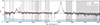 |
Fig. A.1. Power-law fit to the optical continuum of GN-9771, used for the [O III] and Balmer line fitting. We fit a power law to the optical fλ G395H spectrum, using the wavelengths shown as gray shaded regions. Between rest-frame ∼6200 and ∼6300 the lack of data corresponds to the NIRSpec detector gap. |
Appendix B: Balmer lines fitting
In Fig. B.1 we show the best-fit for the Hβ model described in Sect. 3.1, but here we fix the exponential scale of the broad component to the one of the Hα line. As discussed in the formerly mentioned section, by fixing the scale we obtain a fit which is statistically indistinguishable from the best-fit letting this parameter free.
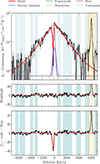 |
Fig. B.1. Same as Fig. 3, but in this case we fixed the exponential scale parameter of the broad component to be the same as in the best fit of Hα (BIC = 68). |
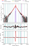 |
Fig. B.2. Same as Fig. 2, but replacing the exponential component with a broad Lorentzian (BIC = 1027). |
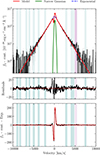 |
Fig. B.3. Same as Fig. 2, but setting the amplitude of the host Gaussian component to zero (BIC = 931). |
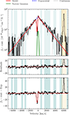 |
Fig. B.4. Same as Fig. 3, but setting the amplitude of the host Gaussian component to zero (BIC = 68). |
Appendix C: [Fe II] fit 6350–8000 Å
In Fig. C.1 we show the [Fe II] fit as described in Sect. 3.3. The fluxes of the fit [Fe II] lines are weaker than in the 4400–6000 Å range, moreover the strongest fit lines are blended with Hα.
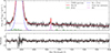 |
Fig. C.1. Zoomed-in image of the G395H spectrum of GN-9771, in the 6350–8000 Å range, containing Hα and He Iλ7067, among other lines. As in Fig. 4, we show the best fit of [Fe II] (green line). |
Appendix D: BH* temperature and electron density
In Fig. D1 we show the Te and ne profiles for photoionized clouds with nH = 1010 cm−3, for different choices of the ionization parameter log10U. All models display qualitatively similar behaviour with a thermalized outer layer with a temperature Te ≈ 6000–7500 K.
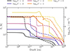 |
Fig. D.1. Temperature-density structure of a suite of BH* models, for varying ionization parameter. Same as Fig. 9, but for a fixed nH = 109 cm−3, for different choices of the ionization parameter log10U. The solid lines indicate temperature (left axis) and the dashed lines indicate electron density (right axis). The ionization parameter mainly influences the temperature of the gas before the ionization front. All the models present a thermalized outer layer with Te ≈ 6000–7500 K, independently of log10U. |
All Tables
Summary of the observed features in the FRESCO-GN-9771 LRD and their interpretation in the context of the black hole star photoionization model.
All Figures
|
Fig. 1. Broadband spectrum of GN-9771 in comparison to other LRDs. We have highlighted the main emission lines on the top axis. We make a comparison with the PRISM spectrum of the other LRDs in our IFU program (Matthee et al. in prep.) and of A2744-45924 (Labbe et al. 2024), after normalizing their flux to match GN-9771 in the 5400–5700 Å band. The spectrum of GN-9771 is very similar to the spectrum of A2744-45924, with only a slightly weaker Balmer break in the case of GN-9771. |
| In the text | |
|
Fig. 2. Triangular P Cygni Hα spectrum of GN-9771. The continuum-subtracted Hα spectrum based on the G395H data is shown in black, whereas the red line shows the best-fit combined model (BIC = 932). Residuals to the model are shown in the middle panel. The fiducial fitting model is described in Sect. 3.1. We indicate the masked regions based on the locations of possible narrow [Fe II] emission in Véron-Cetty et al. (2004) (teal) and He Iλ6680 (purple). The [N II] component is not shown due to its relative flux being negligible. The bottom panel shows the Hα spectrum and best fit after subtracting the exponential component to highlight the P Cygni profile. |
| In the text | |
|
Fig. 3. Hβ spectrum of GN-9771. We used a similar model setup to that for Hα described in Fig. 2 (BIC = 74). The teal regions have been masked due to possible Fe II emission. The orange region indicates the masked [O III] wavelengths. The bottom panel shows the Hβ spectrum and best fit (red) after subtracting the exponential component to highlight the P Cygni profile. Figure B.1 shows a version of the same fit with the exponential scale fixed to that fitted for Hα. |
| In the text | |
|
Fig. 4. [Fe II] forest detected in the G395H data over the ∼5000 Å region of GN-9771. We show the fitted [Fe II] spectrum as described in Sect. 3.3 (green), the He I lines (pink), Hγ (blue dot-dashed), the Hβ model (blue dashed), [O III] λλ4960, 5008 (orange dot-dashed), and [O IIIλ4364 (brown). The residuals of the fit as well as the observational uncertainties on the spectrum are shown in the bottom panel. |
| In the text | |
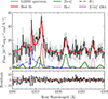 |
Fig. 5. Same as Fig. 4, but zoomed in on the wavelength range containing Hγ and [O III] λ4364. |
| In the text | |
|
Fig. 6. Template fit to UV Fe II. We fit templates to the UV pseudo-continuum emission. The fitting is challenging due to the limited PRISM resolution in this wavelength range (R ∼ 50). The model includes the Mg II and Fe II lines, which are usually strong. The template fitting does not produce a satisfactory result (χν2 = 7.5), in particular for the ∼2500 Å bump. Absorption features from the resonant Fe II multiplets UV1 and UV2+UV3 are compatible with the observed shape of the continuum, which are also predicted by our Cloudy models (see Sect. 6.1 for a discussion). |
| In the text | |
|
Fig. 7. Density and column density of the warm layer as preferred by the [Fe II] line-emission compared to that preferred by the Balmer break strength. The colored contours show the values of χν2 of our fit to the optical [Fe II] of GN-9771 to Cloudy photoionized cloud models with vturb = 210 km s−1 and Z/Z⊙ = 0.01. We also show the strength of the Balmer break for the grid of models as cyan contour lines, where we highlight the approximate Balmer break strength (≈2.5) of GN-9771 with a shaded region. The black line marks the contour of the models with matching [Fe II] EW to the observed in GN-9771, in the range 5100–5400 Å. Dashed lines indicate contours of ×2 difference in EW (increasing toward the right-hand side of the figure). |
| In the text | |
|
Fig. 8. Best-matching BH* model and blackbody fit to the optical spectrum. We matched the gray shaded wavelengths to the larger model grid presented in Naidu et al. (2025). We also show the blackbody that best fits the rest-frame optical (dashed blue) and UV (dashed purple), for which we obtain an effective temperature of TBB, opt = 5753 K (fit to wavelengths highlighted with a gray shade) and TBB, opt = 15 530 K (purple shade), respectively. For illustration, we also include the SED fit to the object ALT-31334 (z = 5.66; M* = 108 M⊙), a typical compact blue galaxy that could resemble a hypothetical host for GN-9771 (see Sect. 6.1). |
| In the text | |
|
Fig. 9. Temperature-density structure of a suite of BH* models. We show the electron temperature (solid lines) and electron density (dashed lines) profiles for models corresponding to log10U = −3, vturb = 210 km s−1 and Z/Z⊙ = 0.01, for a wide range of hydrogen densities. All models are characterized by a hot (∼16 000 K; see Fig. D1 for the temperature with different choices of ionization parameter) and dense ionized region whose temperature and density abruptly drop at an ionization front, its radius dependent on density, and a thermalized outer layer of ∼6000–7500 K. |
| In the text | |
|
Fig. 10. Origins of the lines. The intrinsic emissivity of selected emission lines in the photoionized Cloudy model, for nH = 1010 cm−3, and NH = 1025 cm−2. Emissivities are expressed in arbitrary units of energy per unit time per unit volume. The ionization parameter is log10U = −3. The hydrogen Balmer and helium lines are intrinsically strong in the inner layers due to recombination emission, although the opacity of Hα and Hβ is high, which leads to scattering effects. [Fe II] is mostly emitted in a warm layer with Te = 6000–7500 K, which is shielded from the far-UV ionizing radiation. |
| In the text | |
|
Fig. 11. Density of hydrogen species inside a photoionized slab. We show the volumetric density of fully ionized hydrogen (blue dashed) and first three levels (1s, 2s, 2p) of neutral hydrogen (solid lines) as a function of depth into the photoionized cloud of Fig. 10. Although most neutral hydrogen in the envelope is in the 1s state, there is a significant population (ne ≈ 103 cm−3) of electrons in the 2s state, which produces the Balmer break, and resonant scattering of Balmer lines (N(H I, 2s) ≈1016 cm−2). The high column density of free electrons in the same region could be responsible for electron scattering broadening of the Balmer lines. |
| In the text | |
|
Fig. 12. BH vs. Stellar mass relation for GN-9771. We show estimations of MBH/M* for GN-9771 based on a stellar mass inferred from the dynamical mass suggested by the width of [O III], and MBH estimated using a standard virial relation (empty square; Matthee et al. 2024), and assuming an Eddington luminosity ratio of fEdd = 1 (red square), and fEdd = 10 (cyan square). We make a comparison with the local relation (Reines & Volonteri 2015) and the Illustris-TNG (Weinberger et al. 2017; Pillepich et al. 2018) and EAGLE (Schaye et al. 2015; Crain et al. 2015) simulations at z ≈ 5. We highlight the median trend with a solid (dashed) line and the extrema (95th percentiles) of the distributions in each simulation. |
| In the text | |
|
Fig. 13. Comparable [Fe II] emission in a stack of LRDs. We compare the [Fe II] optical spectrum of GN-9771 with a stack of 13 medium-resolution grating spectra of LRDs. The spectrum of GN-9771 is degraded to the medium resolution of the NIRSpec M-gratings for this comparison. The most luminous [Fe II] lines are detected in the stack, suggesting that these are common among LRDs, although their weak intrinsic fluxes challenge their detection. |
| In the text | |
|
Fig. A.1. Power-law fit to the optical continuum of GN-9771, used for the [O III] and Balmer line fitting. We fit a power law to the optical fλ G395H spectrum, using the wavelengths shown as gray shaded regions. Between rest-frame ∼6200 and ∼6300 the lack of data corresponds to the NIRSpec detector gap. |
| In the text | |
|
Fig. B.1. Same as Fig. 3, but in this case we fixed the exponential scale parameter of the broad component to be the same as in the best fit of Hα (BIC = 68). |
| In the text | |
|
Fig. B.2. Same as Fig. 2, but replacing the exponential component with a broad Lorentzian (BIC = 1027). |
| In the text | |
|
Fig. B.3. Same as Fig. 2, but setting the amplitude of the host Gaussian component to zero (BIC = 931). |
| In the text | |
|
Fig. B.4. Same as Fig. 3, but setting the amplitude of the host Gaussian component to zero (BIC = 68). |
| In the text | |
|
Fig. C.1. Zoomed-in image of the G395H spectrum of GN-9771, in the 6350–8000 Å range, containing Hα and He Iλ7067, among other lines. As in Fig. 4, we show the best fit of [Fe II] (green line). |
| In the text | |
|
Fig. D.1. Temperature-density structure of a suite of BH* models, for varying ionization parameter. Same as Fig. 9, but for a fixed nH = 109 cm−3, for different choices of the ionization parameter log10U. The solid lines indicate temperature (left axis) and the dashed lines indicate electron density (right axis). The ionization parameter mainly influences the temperature of the gas before the ionization front. All the models present a thermalized outer layer with Te ≈ 6000–7500 K, independently of log10U. |
| In the text | |
Current usage metrics show cumulative count of Article Views (full-text article views including HTML views, PDF and ePub downloads, according to the available data) and Abstracts Views on Vision4Press platform.
Data correspond to usage on the plateform after 2015. The current usage metrics is available 48-96 hours after online publication and is updated daily on week days.
Initial download of the metrics may take a while.