| Issue |
A&A
Volume 707, March 2026
|
|
|---|---|---|
| Article Number | A109 | |
| Number of page(s) | 15 | |
| Section | Cosmology (including clusters of galaxies) | |
| DOI | https://doi.org/10.1051/0004-6361/202557660 | |
| Published online | 02 March 2026 | |
Mapping the Perseus galaxy cluster with XRISM
Gas kinematic features and their implications for turbulence
1
Department of Theoretical Physics and Astrophysics, Masaryk University Brno 61137, Czechia
2
Department of Astronomy and Astrophysics, The University of Chicago Chicago IL 60637, USA
3
Center for Astrophysics | Harvard-Smithsonian MA 02138, USA
4
Center for Space Sciences and Technology, University of Maryland, Baltimore County (UMBC) Baltimore MD 21250, USA
5
NASA/Goddard Space Flight Center Greenbelt MD 20771, USA
6
Center for Research and Exploration in Space Science and Technology, NASA/GSFC (CRESST II) Greenbelt MD 20771, USA
7
Max Planck Institute for Astrophysics Karl-Schwarzschild-Str. 1 D-85741 Garching, Germany
8
Space Research Institute (IKI) Profsoyuznaya 84/32 Moscow 117997, Russia
9
Lawrence Livermore National Laboratory Livermore CA 94550, USA
10
Department of Physics, Tokyo Metropolitan University Tokyo 192-0397, Japan
11
Département de Physique, Université de Montréal, Succ. Centre-Ville, Montréal Québec H3C 3J7, Canada
12
RIKEN Nishina Center Saitama 351-0198, Japan
13
Faculty of Physics, Tokyo University of Science Tokyo 162-8601, Japan
14
IRAP, CNRS, Université de Toulouse, CNES, UT3-UPS Toulouse, France
15
Kavli Institute for Astrophysics and Space Research, Massachusetts Institute of Technology Cambridge MA 02139, USA
16
Faculty of Engineering, University of Miyazaki Miyazaki 889-2192, Japan
17
College of Science and Engineering, Kanto Gakuin University Kanagawa 236-8501, Japan
18
Department of Astronomy, University of Maryland, College Park MD 20742, USA
19
Faculty of Mathematics and Physics, Kanazawa University, Kanazawa Ishikawa 920-1192, Japan
20
Advanced Research Center for Space Science and Technology, Kanazawa University, Kanazawa Ishikawa 920-1192, Japan
21
Academia Sinica Institute of Astronomy and Astrophysics (ASIAA) Taipei 106319, Taiwan
★ Corresponding author: This email address is being protected from spambots. You need JavaScript enabled to view it.
Received:
11
October
2025
Accepted:
4
December
2025
Abstract
We present extended gas kinematic maps of the Perseus cluster based on a combination of five new XRISM/Resolve pointings observed in 2025 with four performance verification datasets from 2024, totaling a net exposure of 745 ks. To date, Perseus remains the only cluster that has been extensively mapped out to ≃0.7r2500 by XRISM/Resolve, while simultaneously offering sufficient spatial resolution to resolve gaseous substructures driven by mergers and active galactic nucleus (AGN) feedback. Our observations cover multiple radial directions and a broad range of dynamical scales, enabling us to characterize the kinematic properties of the intracluster medium up to a scale of ∼500 kpc. In the measurements, we detected high-velocity dispersions (≃300km s−1) in the eastern region of the cluster that are spatially coincident with the extended X-ray surface brightness excess and correspond to a nonthermal pressure fraction of ≃7 − 13%. The velocity field outside the AGN-dominant region can be effectively described by a single, large-scale kinematic driver based on the velocity structure function, which statistically favors an energy injection scale of at least a few hundred kpc. The estimated turbulent dissipation energy is comparable to the gravitational potential energy released by a recent merger, implying a significant role of turbulent cascade in the merger energy conversion. In the bulk velocity field, we observed a dipole-like pattern along the east-west direction with an amplitude of ≃ ± 200 − 300 km s−1, indicating rotational motions induced by the recent merger event. This feature constrains the viewing direction to ≃30° −50° relative to the normal of the merger plane. Our hydrodynamic simulations suggest that Perseus has experienced at least two energetic mergers since redshift z ∼ 1, the most recent of which is associated with the radio galaxy IC310, in agreement with recent SRG/eROSITA findings. This study showcases exciting scientific opportunities for future missions with high-resolution spectroscopic capabilities (e.g., HUBS, LEM, and NewAthena).
Key words: turbulence / methods: observational / techniques: imaging spectroscopy / galaxies: clusters: intracluster medium / galaxies: individual: Perseus / X-rays: galaxies: clusters
© The Authors 2026
 Open Access article, published by EDP Sciences, under the terms of the Creative Commons Attribution License (https://creativecommons.org/licenses/by/4.0), which permits unrestricted use, distribution, and reproduction in any medium, provided the original work is properly cited.
This article is published in open access under the Subscribe to Open model. This email address is being protected from spambots. You need JavaScript enabled to view it. to support open access publication.
1. Introduction
The Perseus cluster is a prototypical cool-core galaxy cluster system that hosts a variety of remarkable gaseous structures (e.g., shocks, cold fronts, bubbles, and turbulent fluctuations) that have been studied extensively with all major X-ray telescopes (e.g., Forman et al. 1972; Schwarz et al. 1992; Fabian et al. 2000; Churazov et al. 2003; Simionescu et al. 2012; Zhuravleva et al. 2015; Hitomi Collaboration 2016) as well as in other wavelength observations (e.g., Salomé et al. 2006; Canning et al. 2014; Gendron-Marsolais et al. 2020; van Weeren et al. 2024; Cuillandre et al. 2025). It has been widely regarded as a textbook example of radio-mode active galactic nucleus (AGN) feedback and merger-driven sloshing, which are two major physical processes shaping cluster gas atmospheres (i.e., the intracluster medium, ICM), especially the central region (see Markevitch & Vikhlinin 2007; Fabian 2012; Zuhone & Roediger 2016 for reviews). In theoretical studies, Perseus often serves as a diagnostic benchmark for models of AGN feedback and microphysics of the ICM implemented in numerical simulations (e.g., Reynolds et al. 2005; Li & Bryan 2014; Zhang et al. 2022; Ewart et al. 2024).
The dynamical state and assembly history of the Perseus cluster have long been the subject of investigations (e.g., Simionescu et al. 2012; Kang et al. 2024; Churazov et al. 2026), as they are essential for understanding the formation of X-ray and radio structures (e.g., cold front edges at different radii, co-existence of radio halos of various types, etc.), the dynamical impact of AGN feedback throughout the entire cool core, and the secular evolution of member galaxies. Direct gas velocity measurements are expected to offer critical insights into these processes (see Simionescu et al. 2019 for a review).
Hitomi pioneered the high-resolution, non-dispersive imaging spectroscopy of the hot cluster atmosphere in Perseus, detecting gas motions with the velocity dispersion ≃80 − 220 km s−1 within the radius of ≃60 kpc, ∼1/3 of the cool-core radius (Hitomi Collaboration 2016, 2018). The recently launched XRISM observatory is equipped with the Resolve X-ray microcalorimeter, which offers a high energy resolution of ≃4.5 eV at full width at half maximum (FWHM; Tashiro et al. 2021; Ishisaki et al. 2022). It is designed to carry forward the mission initiated by the short-lived Hitomi, reopening the window into the high-precision ICM kinematics.
The X-ray microcalorimeter enables the spatial mapping of the ICM kinematics, which is critical for characterizing mass and energy flows in galaxy clusters and essential for understanding cluster assembly processes and the plasma physics of the ICM (e.g., Kitayama et al. 2014; Zhang et al. 2024). However, Resolve’s moderate angular resolution of ≃1.3′ (half-power diameter, HPD) and relatively small effective area (i.e., ≃200 cm2 at 6 keV) practically require the mapping target to be nearby and sufficiently bright. Perseus, being the brightest cluster in the X-ray sky and located at a low redshift, is thus an optimal target for the goal.
As one of the XRISM’s performance verification (PV) targets, Perseus was observed along an NW arm of four pointings in February 2024 (see Fig. 1; XRISM Collaboration 2025e). The gas velocity radial profiles were measured up to the radius of ≃250 kpc, enabling us to unambiguously disentangle at least two dominant gas kinematic drivers operating on distinct spatial scales (XRISM Collaboration 2025e). The small-scale driver, confined within the central ≲60 kpc of the cluster, is associated with AGN feedback; while the large-scale one (likely a few hundred kpc or even larger) dominates the outer region, driven by mergers of clusters. XRISM Collaboration (2025e) provided a lower limit of the energy injection scale, ≃100 kpc, of the outer driver. A tighter constraint requires the velocities to be mapped over a broader region.
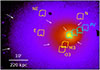 |
Fig. 1. XRISM/Resolve pointings used in this work, labeled with their region names. The background shows the XMM-Newton X-ray surface brightness in the 0.5 − 3.5 keV band (Churazov et al. 2026). White arrows indicate the sloshing cold fronts identified in the system (e.g., Walker et al. 2018). The pointings E, NE, and N (calibration), together with M3 and O3 (GO cycle 1 observations), are newly reported in this work, marked in yellow (see Sect. 2). |
This paper reports five additional XRISM/Resolve pointings of the Perseus cluster observed in 2025 (see Fig. 1 as well as Table 1). Combined with the PV data (observed in 2024), we present an extended, up-to-date velocity map. Perseus is currently the only XRISM cluster target with extensive mapping from its core region out to larger radii (a few hundred kpc), while still offering sufficient spatial resolution to resolve gaseous substructures (c.f., A2029, see XRISM Collaboration 2025b). The coverage across a broad range of dynamical scales (i.e., ≃50 − 500 kpc) and radial directions (E+NE, NW, and W) enables a robust characterization of the velocity field, shedding lights on physical properties of the dominant gas kinematic sources.
In this work, we focus on large-scale, merger-associated motions and show that their statistical features (e.g., velocity structure function, turbulent heating rate, etc.) can be effectively described by a velocity field dominated by a single, large-scale kinematic driver. The velocity measurements confirm the significant role of the turbulent cascade in merger energy conversion (from the gravitational to thermal energies). Our velocity maps also provide strong constraints on the merger scenario and viewing angles of the system, complementing other X-ray and weak-lensing measurements (Churazov et al. 2026; HyeongHan et al. 2025). This study highlights the scientific value of mapping the ICM and lays the groundwork for future projects and missions (e.g., XRISM key or legacy projects: HUBS, LEM, and NewAthena; see Cui et al. 2020; Kraft et al. 2022; Cruise et al. 2025) aimed at mapping gas kinematics in nearby clusters with long exposures.
This paper is organized as follows. Section 2 outlines the XRISM/Resolve observations and data reduction. Section 3 presents the extended velocity maps of Perseus. Section 4 characterizes the velocity fields and their physical properties. Section 5 constrains the merger configuration of the cluster using the velocity map. Finally, Sect. 6 summarizes our main conclusions. Throughout the paper, we assume a flat cosmology with H0 = 67 km s−1 Mpc−1 and Ωm = 0.32, with 1′ = 22 kpc at the cluster redshift (z ≃ 0.017).
2. XRISM/Resolve observations and data analysis
The Perseus cluster was observed multiple times during January/Feburary and July 2025 for calibration purposes and general observer (GO) project (Cycle 1, PI: I. Zhuravleva; see Fig. 1 and Table A.1). Our data reduction and modeling largely follow the descriptions in XRISM Collaboration (2025e), but using the latest versions of the HEASoft (v6.35.2), CalDB (v20250315), and AtomDB (v3.1.3). The analysis was confined to the highest-resolution primary (Hp) events, providing spectral resolution of ≃4.5 eV (FWHM). The pixel 27 was excluded due to its gain drift issue (Porter et al. 2024).
Our spectra were extracted from the sub-FOV for four PV pointings or from the full FOV for calibration and GO pointings. Both source and background spectra were grouped to ensure at least one count per energy bin. For each region, we generated the corresponding L-size redistribution matrix file (RMF) and auxiliary response files (ARFs). We used an XMM-Newton image in the ARF generation for the calibration and GO pointings, as some of them are not covered by Chandra data.
The grouped spectra were then fitted in the 3 − 11 keV energy range using a model that included the ICM, non-X-ray background (NXB), and (if necessary) AGN components. The ICM emission was modeled as a single-component spectrum from optically thin plasma in collisional ionization equilibrium (bvapec model in Xspec v12.15.0), absorbed by the foreground along the line of sight (LOS) with a fixed equivalent hydrogen column density of nH = 1.38 × 10⁻²¹ cm−2 (Willingale et al. 2013). The Fe Heα resonance (ω) line was excluded from the bvapec (see Appendix A.6) and modeled separately with a redshifted Gaussian. Its redshift and width were both linked to the ICM component for all regions outside 60 kpc.
For the PV data, we adopted the same spatial binning scheme as XRISM Collaboration (2025e, see their Extended Data Fig. 3). A correction for the point spread function (PSF) effect (a.k.a., spatial-spectral-mixing, or SSM) was fully implemented (same as in XRISM Collaboration 2025e), which is particularly crucial for the radially connected regions with steep X-ray surface brightness gradients (e.g., central regions of the cool-core clusters). We confirm that our new fitting results are fully consistent with XRISM Collaboration (2025e) within the 1σ uncertainty, despite the updated calibration and atomic databases.
For the calibration and GO data (newly reported in this work), we omitted the SSM correction due to the widely scattered sky positions of their pointings and tied all abundances (except He) to Fe as the emission lines from the non-Fe elements are relatively faint. Since these pointings are all located at least 5′ away from the bright cluster center, they are much less affected by the SSM compared to the inner PV pointings, which is further confirmed with the Resolve raytracing simulations (see Sect. 3). We examined the SSM correction between M3 and O3. Its effect on velocity measurements are smaller than 1σ statistic uncertainty. The best-fit ICM parameters are summarized in Table 1. The outermost pointings, E and NE, have relatively shallow exposures but exhibit consistent velocities. We therefore combined them (denoted as E+NE) to measure the averaged velocities near the E and NE regions (see Fig. A.3 for a comparison between the joint and separate fittings). Unless stated otherwise, we only used this joint measurement for E and NE for the rest of the study. Our conclusions would remain largely unaffected if the NE region were to be excluded from the analysis instead.
We specifically examined the regions with high-velocity dispersion for evidence of multiple temperature and velocity components. The E region shows a tentative indication of such complexity – a ∼2 − 3σ deviation near the Fe Lyα lines, suggesting an additional, more redshifted, hotter component. A similar trend is seen in the region NE, but the data is considerably noisier. No significant sign of multiple components is found in other regions. In Fig. 2, we compare the best-fit models with one-temperature (1T) and two-temperature (2T) components for the region E. A combination of cold (kBT ≃ 4.0 ± 0.4 keV) and hot (kBT ≳ 9 keV) components slightly improve the fit of the Fe Lyα lines (see Appendix A.5 for more details). The cold component dominates the Fe Heα line flux with σlos ≃ 290 ± 0 km s−1 and ulos ≃ 200 ± 70 km s−1, consistent with our 1T result within ≃2σ (see the pink cross in Fig. 4), while only an upper limit was obtained for the hot component’s dispersion (≃250 km s−1) and a lower limit for the temperature. Deeper observations are required to confirm the result and to better separate the components if present. In this study, we focus on the 1T measurements for all regions unless noted otherwise, but also discuss how the potential temperature complexity in E and NE may influence our conclusions.
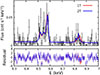 |
Fig. 2. Fe Heα and Lyα lines in the E region with best-fit 1T and 2T models. The spectrum suggests the presence of an additional, more redshifted, hotter component, which would have to be confirmed with deeper observations. Residuals normalized by the statistical errors, i.e., (data-model)/error, are displayed in the lower panel (see Sect. 2 and Appendix A.5). |
3. Gas kinematic maps of Perseus
Figure 3 shows our extended velocity maps of the hot ICM in Perseus, assuming a single-temperature component, based on four PV, three calibration, and two GO pointings1. We used the built-in HEASoft tool xmatraceback to trace the sky region contributing scattered photons to each detector region where we extracted spectra. In Fig. 3, the color patches indicate the sky regions that contribute 50% of the photons for their corresponding detector regions, approximately reflecting the areas where we measured the velocities. The confidence levels for our velocity measurements are presented in Fig. 4. The pink cross shows the cold component in the 2T model of the region E for comparison.
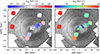 |
Fig. 3. Best-fit gas bulk velocity (left) and velocity dispersion (right) maps of the Perseus cluster from nine XRISM/Resolve pointings. The maps are centered on the Perseus center (RA = 49.9507, Dec = 41.5117). The N and NE regions show the E+NE joint fitting result assuming a single temperature model. The color patches indicate the sky areas that contribute 50% of the photons for the corresponding sub-regions based on raytracing simulations. The measurement uncertainties are shown in Fig. 4. The Chandra X-ray residual is overlaid in the background highlighting the inner sloshing spiral and the eastern X-ray surface brightness excess, with black circles marking radii of 100, 200, and 300 kpc. The bulk velocity distribution, in the rest frame of the central ICM (zicm = 0.017628), shows an (asymmetric) dipole-like pattern, revealing a rotational motion of the ICM (see Sect. 3). |
The left panel of Fig. 3 shows the LOS bulk velocity with a heliocentric correction in the rest frame of the central ICM, zICM = 0.017628, measured within ≃30 kpc (the central pointing; see XRISM Collaboration 2025e). Such a rest frame is selected to highlight gaseous substructures in the Perseus core, which does not affect any conclusions in the paper. We note that the redshift of the brightest cluster galaxy (BCG) stellar component is zBCG = 0.017284 (Hitomi Collaboration 2018), corresponding to ≃ − 103 km s−1 velocity offset relative to the central ICM. An asymmetric dipole-like structure is visible in the bulk velocity distribution, where the most positive (moving away from us) and negative (toward us) velocities are located on the opposite sides of a symmetry axis oriented near the north-south direction. It implies a gas bulk rotation on a scale of at least ∼400 kpc, associated with the recent merger processes. Interestingly, the circumnuclear disk in Perseus is rotating along a similar direction on much smaller scales (< 0.1 kpc; see Nagai et al. 2019). In Sect. 5, we describe how we used this dipole-like feature to constrain sloshing configuration and viewing angles of the system. Sanders et al. (2020) mapped the bulk velocity of Perseus over a ∼600 kpc radial range with XMM-Newton observations by calibrating the energy scale of the EPIC-pn detector, but the statistical uncertainties are relatively large – typically ≳200 km s−1 (1σ; see their fig. 16) and ≳300 km s−1 near our E, NE, and N regions.
The right panel of Fig. 3 shows the velocity dispersion map. The region E+NE exhibits the highest velocity dispersion detected so far in Perseus (with > 3σ significance), suggesting strong gas random motions and high nonthermal pressure (see Sect. 4.1) in its vicinity. Coherent bulk motions (especially overlapping velocity shears near sloshing cold fronts or merger shocks) can contribute to the velocity dispersion. However, there are no clear signs of such structures from high-resolution X-ray images, aside from an extended X-ray surface brightness excess in the nearby regions (see Appendix A.5 for a discussion on multiple temperature components). Interestingly, the O3 region, partially overlapping with the eastern excess, also shows a high-velocity dispersion, which hints at the chaotic behavior of the X-ray excess and its connection with the recent mergers.
4. Characterizing the kinematic properties
The gas velocity field offers valuable insights into the assembly history of the Perseus cluster and its ICM properties. In this section, we characterize the statistical properties of our velocity measurements and discuss their physical implications. We caution that the statistical significance of our findings remains limited by the current spatially sparse velocity sampling. Additional XRISM observations with a more uniform mapping configuration will be essential to confirm these findings.
4.1. Nonthermal pressure
The nonthermal pressure fraction (fnth), namely, the ratio of kinematic to total pressure in the ICM, characterizes the dynamical significance of gas random motions and the extent to which the cluster atmosphere deviates from hydrostatic equilibrium (e.g., Evrard 1990; Nagai et al. 2007; Lau et al. 2009; Shi & Komatsu 2014). Assuming isotropic velocity fields and the LOS velocity dispersion predominantly reflects gas random motions, the nonthermal pressure fraction solely depends on the 1D Mach number M1D (≡σlos/cs), expressed as
 (1)
(1)
where  is sound speed; γ ( = 5/3), μ ( = 0.6), and mp are the adiabatic index of monatomic gas, mean molecular weight per ion, and proton mass, respectively. We note that anisotropies in the velocity field induced by gravitational stratification and magnetic fields (e.g., Shi & Zhang 2019; Hu et al. 2025) could potentially affect the characterization. In addition, the true nonthermal pressure contribution can be underestimated due to the X-ray emissivity weighting (e.g., Vazza & Brunetti 2026 and see also Fig. 7).
Thus far, most XRISM cluster studies suggest low nonthermal pressure contributions in the cluster cores (e.g., ≃1 − 4%) along the LOS across the center of the Coma Cluster, Centaurus, A2029, and Ophiuchus (XRISM Collaboration 2025d,c,a; Fujita et al. 2025). Interestingly, deep off-center observations of A2029 reveals a decreasing nonthermal pressure fraction with the radius up to at least r2500 along the NE direction2. This is in contrast to cosmological simulation predictions, in general, despite the fact that A2029 is known as one of the most relaxed clusters in observations.
Perseus is the second cluster for which we attempt to measure the nonthermal pressure profile out to approximately 0.7r2500 after A2029, where r2500 ≃ 570 kpc in Perseus (de Vries et al. 2023). The results are shown in Fig. 5, where fnth ranges from ≃0.5 − 5%, comparable to values observed in most other XRISM clusters, except in the inner- and outermost regions (≳10%) and in O3 (≃7%). The innermost region is strongly influenced by radio-mode AGN feedback (e.g., jets, bubbles). The four neighboring regions within the annulus R ≃ 10 − 60 kpc show azimuthal variations by a factor of ∼6 (see Fig. 3), plausibly also associated with the central supermassive black hole (SMBH) activities (see more discussions in XRISM Collaboration 2025e). We note that there are potential systematic uncertainties induced by the imperfect PSF calibration, which tend to have a stronger impact on smaller detector regions. Although XRISM Collaboration (2025e) showed that 30% off-axis ARF uncertainties affect velocity measurements still within their 1σ statistic errors (see their extended data fig. 4), the impact might depend on specific spatial regions and binning schemes.
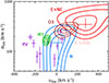 |
Fig. 4. 2D confidence contours (1, 2, and 3σ) of the bulk velocity and velocity dispersion measurements of our new regions (calibration and GO pointings). The red contours indicate a joint fit between the E and NE regions (see Fig. A.3 for their individual fits). The crosses mark the best-fit parameters and their 1σ uncertainties, including also all PV data (ten sub-regions; see Sect. 3). The pink cross indicates the cold ICM component in the 2T model for region E (see Sect. 2). |
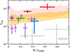 |
Fig. 5. Nonthermal pressure fraction profile of the Perseus cluster, compared with A2029 (grey points; XRISM Collaboration 2025b). Colors follow the same scheme as in Fig. 4 for Perseus. The shaded bands show numerical predictions from TNG cosmological simulations for two cluster subsamples: (i) the 31 most relaxed clusters from the TNG-300 simulation suite (yellow) and (ii) 30 Perseus-like massive, cool-core clusters from TNG-Cluster suite (pink). The bands represent the 10th-90th percentile range of the fnth distribution within each sample. The inner AGN-dominant region, as well as the regions overlapping the eastern X-ray surface brightness excess (E+NE and O3), show high fnth (> 7%; see Sect. 4.1). |
The E+NE and O3 regions exhibit the highest nonthermal pressure fractions in the current Perseus measurements. In the 2T model of region E, the dominant cold component yields fnth ≃ 11 ± 5%, consistent with the 1T fit. Perseus is often considered a relaxed system, yet it also shows active AGN feedback and prominent sloshing features in its X-ray distribution. For comparison, we show numerical predictions based on the IllustrisTNG cosmological simulations in Fig. 5 (Pillepich et al. 2018; Springel et al. 2018; Naiman et al. 2018; Marinacci et al. 2018; Nelson et al. 2018, 2019). They are estimated based on the X-ray-weighted velocity dispersion for a direct comparison with observations. Two subsamples of the TNG clusters were considered. One consisted of the 31 most relaxed clusters from the TNG-300 simulation suite, selected based on the spherical gas morphology and absence of substructures, with masses ranging 1 − 7 × 10¹⁴ M⊙ (yellow; see Zhang et al. 2024 for details). The other consisted of 30 Perseus-like clusters from the TNG-Cluster suite (Nelson et al. 2024), selected based on their halo mass (5 − 10 × 1014 M⊙) and the presence of cool cores (pink; see Truong et al. 2024; XRISM Collaboration 2025f). The shaded bands indicate the 10th and 90th percentiles of the fnth scatter within each sample. The Perseus-like clusters from the TNG-Cluster exhibit systematically higher nonthermal pressure fraction than the relaxed cluster sample. Observationally, Perseus resembles the relaxed sample within ≃0.2r2500 (excluding the innermost region), with values that are markedly lower than those of its massive, cool-core numerical counterparts. The same holds for the entire NW arm. Beyond 0.2r2500, only the two regions overlapping with the eastern X-ray excess show higher fnth than the relaxed sample, consistent with the TNG-Cluster one.
We further compare Perseus and A2029 – the two clusters with the most extended nonthermal pressure measurements to date and with comparable effective length radial profiles (see Fig. A.2). The effective length characterizes the region size along the sightline that contributes majority of the X-ray flux (Zhuravleva et al. 2012; see also Appendix A.3). The measured velocity dispersion depends on the effective length ℓeff along the LOS. In observations, a fair comparison of fnth is possible only when the clusters (or regions) being compared have similar ℓeff.
Perseus and A2029 share a collection of similar gaseous features shaped by AGN-driven bursts and mergers. They both exhibit prominent radio lobes (on ∼10 and 30 kpc scales, respectively) powered by their central SMBHs (e.g., Timmerman et al. 2022), as well as sloshing spirals within ≃200 kpc (∼0.3r2500). These similarities partially explain the comparable fnth of the two clusters within the radial extent of their inner sloshing spirals. Beyond the spiral, however, the velocity dispersion in A2029 drops rapidly (XRISM Collaboration 2025b), in contrast to the case of Perseus. Overall, this difference reflects the more complex merger history of Perseus. Simulations suggest that a minor merger occurred ∼2 − 3 Gyr ago in A20293, whose sloshing spiral has not yet fully developed (see also Sohn et al. 2019). In Perseus, the inner and outer sloshing cold fronts may have been driven by separate mergers, with a ∼3 − 5 Gyr time interval, resulting in a more turbulent atmosphere outside the cool core than in A2029 (see Sect. 5).
4.2. Velocity structure function and injection scales
The velocity structure function is an essential diagnostic tool for characterizing gas motions utilizing the LOS bulk velocity map. It quantifies the velocity differences between spatially separated regions, thereby probing directly the scale dependence of turbulent flows (e.g., Zhuravleva et al. 2012; Miniati 2014; ZuHone et al. 2016; Zhang et al. 2024; Gatuzz et al. 2023). This method was applied to the recent XRISM observations of the Coma cluster and tentatively revealed a sign of extremely steep velocity power spectrum (XRISM Collaboration 2025d); however, the question of whether it reflects cosmic variance and/or inhomogeneity in the velocity field is still under debate (Vazza & Brunetti 2026).
The nine pointings of Perseus provide the most powerful dataset to date for a similar analysis (c.f., two pointings in Coma). Perseus, however, is a cool-core cluster, exhibiting strong X-ray surface brightness gradients that modulate the observed structure function. XRISM Collaboration (2025e) also suggested the presence of at least two drivers within the Perseus cool core. Therefore, in our estimation, we only adopted the region beyond R ≃ 60 kpc to avoid the impact of AGN feedback (one of the dominant drivers). To interpret the measurements, we generated Gaussian random velocity fields with underlying energy power spectra E(k) as baseline models, expressed as
 (2)
(2)
where E0 is a normalization factor, ℓinj is the energy injection scale, and ℓdiss is a sufficiently small dissipation scale (≪ℓinj, fixed at 1 kpc in this study), while α and β are the spectral indices within the inertial range (α = −5/3 if Kolmogorov turbulence, see Kolmogorov 1941) and at large scales (> ℓinj), respectively. Subramanian et al. (2006) suggested β ≃ 2 as the ICM is mildly compressible, but it might be sensitive to the detailed physics of the system (e.g., gravitational stratification). A similar approach was applied in the study of the Coma cluster (XRISM Collaboration 2025d). The cluster environment can be far more complicated than isotropic turbulence (see Hosking & Schekochihin 2022 and references therein for a detailed discussion of the latter situation). We project the 3D Gaussian random velocity field along the LOS, assuming Perseus-like X-ray emissivity distribution. To examine the effect of gravitational stratification on turbulence evolution, we further ran “turbulence-in-a-box” simulations, similar to those performed in XRISM Collaboration (2025e), and found little difference between the simulations and the Gaussian model regarding the shape of the velocity structure function (see Appendix B for more details).
Figure 6 shows the second-order velocity structure function constructed from both observations and Gaussian models, namely,
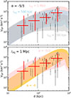 |
Fig. 6. Second-order velocity structure function for the velocity field outside the AGN-dominant region (≳60 kpc) in Perseus, grouped into four bins (red points). Black points show all available velocity pairs with their 1σ statistical uncertainties. The shaded regions show theoretical predictions and their 68% scatters based on Gaussian random fields. Various energy injection scales (top) and spectral indices are shown to compare with the observations. The XRISM Perseus dataset favors a large injection scale (at least a few hundred kpc) but is not sensitive to the spectral index (see Sect. 4.2). |
 (3)
(3)
where ⟨⟩ denotes an average over all velocity pairs on the sky with spatial separation d (=|d|). The black points represent all available velocity pairs derived from our velocity map, while the error bars correspond to 1σ statistical uncertainties in the measurements. To estimate the structure function, we grouped these velocity pairs into four separation bins, shown as the red points. We also tested three and five bins, which yielded similar results. To evaluate the uncertainties, we performed a Monte Carlo sampling of all velocity differences within each bin. The presented error bars enclose the 68% scatter range, accounting for both variations in the velocity differences and their measurement errors. Our theoretical predictions are overlaid as shaded bands, indicating a 68% level of scattering that reflects the cosmic variance based on 200 random realizations. We experimented with various energy injection scales (top panel) and spectral indices (bottom panel). We did not fit the velocity normalization but adjusted it to visually match the measurements. Our models were derived from the X-ray-weighted bulk velocity within R = 60 − 400 kpc, a radial range consistent with the observations. We also tested estimating VSF from regions similar to those in the observations, which resulted in consistent structure functions overall. However, we emphasize that, in both cases, our models contain far more velocity pairs than the observations. The current data may therefore be affected by cosmic variance.
A single, large-scale driver can effectively reproduce the observations. It corresponds to the outer, merger-associated driver proposed by XRISM Collaboration (2025e) in their “double-cascade scenario,” which can be a combination of multiple drivers as long as they all operate at large scales. Our measurements favor a large injection scale (ℓinj ∼ 500 kpc or even larger), broadly consistent with cosmological simulation predictions (e.g., Norman & Bryan 1999; Vazza et al. 2009; Miniati 2014; Zhang et al. 2024). The bin with the largest separation provides the strongest constraint, with 7 out of 15 velocity pairs lying above the 1σ limit (84%) of the ℓinj = 200 kpc prediction. Assuming the pair distribution is Gaussian and independent, our measurements can rule out ℓinj = 200 kpc at a confidence level of ≳99.5%. Although the model of ℓinj = 200 kpc can be shifted vertically to match data better at large separations, it will lead to an unrealistic velocity amplitude. We note that regions E+NE contribute dominantly to the bin with d ≳ 300 kpc. If the presence of multiple temperature components is confirmed, additional complexity arises. Excluding E/NE from our velocity structure function estimation, we cannot rule out ℓinj = 200 kpc based on the remaining dataset. XRISM Collaboration (2025e) used the velocity dispersion dip near R ≃ 60 − 100 kpc along the NW direction to place a lower limit of the ℓinj (≳100 kpc). Their argument is that the ℓinj cannot be smaller than the local effective length scale, otherwise the radial profile of the velocity dispersion would be flat. We confirm this result with the velocity structure function independently and our new data slightly improve their constraint. Since information at larger separations (e.g., 1 Mpc) is critical to examining ℓinj = 200 − 500 kpc, future observations to the west and southwest of the cluster will provide key additional insights.
We also tested a very steep spectrum inspired by the recent Coma measurements (XRISM Collaboration 2025d) to consider it as a possible source of a large dissipation scale (≳240kpc). However, our measurements cannot distinguish it from the Kolmogorov scaling due to the insufficient number of velocity pairs with small separations. In XRISM Collaboration (2025d), bulk velocity and velocity dispersion were combined to constrain the velocity power spectrum. We defer such an analysis to future work owing to the complex surface brightness stratification in Perseus.
4.3. Turbulent heating rate and dissipation energy
Given the suggested large energy injection scales, we estimated the turbulent heating rate following XRISM Collaboration (2025e), namely,
 (4)
(4)
where C0 is a constant coefficient, ρgas is the gas mass density averaged along the LOS, and ℓeff is the effective length (see Appendix A.3). The X-ray emissivity distribution plays a role as a velocity high-pass filter, so that the measured X-ray-weighted σlos reflects gas motions on the scale of ℓeff or smaller. In a turbulent cascade scenario, gas kinetic energy within the atmosphere is dominated by motions on the largest scales (see a sketch in Fig. 7). Equation 4 is valid for motions with ℓinj ≳ ℓeff, which is likely the situation for mergers. The denominator in Eq. (4), however, needs to be replaced by the turbulent energy injection scale ℓinj when ℓinj < ℓeff, a possible situation in the AGN-feedback-dominant region (see more discussions in XRISM Collaboration 2025e). We adopted C0 = 5, calibrated by laboratory experiments and direct numerical simulations of hydrodynamic turbulence (see Zhuravleva et al. 2014 and references therein). Its exact value is not critical for our order-of-magnitude estimations, as long as it remains within an order of unity.
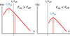 |
Fig. 7. Effect of X-ray emissivity distribution on modulating the dominant velocity power spectrum we probe. The X-ray emissivity acts as a velocity high-pass filter, allowing us to probe only the largest scales smaller than 1/ℓeff in k-space (see Appendix A.3 for definition and calculation of ℓeff). The pink regions depict the range of spatial scales that dominate the gas kinematic energy in the measurements. In this work, we focus on merger-driven, large-scale gas motions, which are likely to correspond to the situation shown on the left (see Sect. 4.3). |
The estimated heating-rate radial profile is shown in Fig. 8. The error bars include both the statistical uncertainties (1σ) of the velocity dispersion measurement and the spatial variations of the effective length (and their uncertainties) within each region. We assume the dominant injection scale is larger than or comparable to the maximum ℓeff within our radial coverage (∼500 kpc; see Table 1), which is supported by the velocity structure function discussed in Sect. 4.2. The radial profile of the heating rate is strongly peaked at the cluster center and flattens outside R ≃ 60 kpc, forming a plateau that extends to the maximum radius we probe (see XRISM Collaboration 2025e for more discussions on the central peak associated with the AGN heating). Within the still-large uncertainties, all regions in the plateau are consistent with a uniform heating rate of approximately 10−28 − 10−27 erg cm−3 s−1 (estimated visually), though the regions near the far end of the NW arm appear lower. A defining feature of Kolmogorov-like turbulence with a single injection scale is the assumption of a constant heating rate within the inertial range (Kolmogorov 1941). Our measurement does not significantly deviate from this scenario. This consistency is generally in line with the fact that most of the kinetic energy is released during the early stage of a merger (e.g., within the first dynamical timescale). The turbulence decays over a much longer timescale. Both ℓinj and its corresponding velocity amplitude (σinj) evolve with time and the eddy turnover timescale Δtturnover (=ℓinj/σinj) increases as ∼t, independent of the spectral slope on large scales (i.e., β in Eq. (2), see Subramanian et al. 2006).
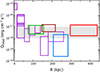 |
Fig. 8. Radial profile of the turbulent heating rate. The color scheme is the same as in Fig. 4. The uncertainties incorporate both the velocity statistical errors and effective length variations within each region. Outside the AGN-dominant region (i.e., ≳60 kpc), the heating rate appears approximately uniform (∼10−28 − 10−27 erg cm−3 s−1, marked by the grey band), covering a dynamical range of ℓeff ≃ 100 − 400 kpc (see Sect. 4.3). |
We can then characterize the contribution of turbulent dissipation in the merger energy budget. The turbulent dissipation energy can be approximated as
 (5)
(5)
In the early stage of a merger, ℓinj reflects either the size of the infalling subhalo or the characteristic scale of its orbit. Under an assumption of the Kolmogorov scaling, namely, σinj = (ℓinj/ℓeff)1/3σlos within the inertial range, the equation is further expressed as
 (6)
(6)
If the energy power spectrum is close to the form of Eq. (2), Ediss scales as t(4 − 2β)/(3 + β), remaining time-independent for β = 2, in which case the measured Ediss is temporally representative (Subramanian et al. 2006). We argue that even if Ediss evolves with time, our estimate is likely close to an average over the entire merger period, since the σlos implies a reasonable dissipation timescale as Δtturnover ≃ 2, 4, 3, and 2 Gyr from the region E+NE, N, M3, and O3, assuming ℓinj = 1 Mpc. For reference, the Perseus’s dynamical timescale is  , where G is the gravitational constant, M200 (≃6 × 10¹⁴ M⊙) and r200 (≃1.8 Mpc) are the virial mass and virial radius of Perseus, respectively. A merging cluster generally requires a ∼3 − 4 dynamical timescale to dissipate its kinetic energy and relax (e.g., Poole et al. 2006). As a comparison, the situation in A2029 is different. Its outer pointings correspond to Δtturnover ≃ 8 Gyr, assuming the same ℓinj as in Perseus, which is likely to be a lower limit only. This implies that the gas environment outside the sloshing spiral in A2029 has been largely settled after an earlier merger event.
The XRISM measurements suggest Ediss ∼ 1062 − 1063 erg in Perseus, an order-of-magnitude estimation. It can be compared with the gravitational energy released through a merger into the ICM of Perseus,
 (7)
(7)
where fgas (≃0.17) is the gas fraction of the cluster and ξ is the merger mass ratio. A merger with ξ ≃ 3 − 10 (as suggested in Sect. 5, see also Bellomi et al. 2024) results in Egrav ≃ 3 × 1062 − 1063 erg, comparable to Ediss, implying the significant role of turbulent dissipation in the merger energy conversion. This is in line with theoretical expectations (e.g., Vazza et al. 2011; Miniati & Beresnyak 2015; Shi et al. 2020). XRISM/Resolve, for the first time, enables this kind of observational investigation.
Finally, we note that the validity of our estimation depends on whether the observable, σlos, reflects the strength of the gas random motions. It is a reasonable assumption for the systems such as Perseus. The most recent merger in Perseus occurred 3 − 5 Gyr ago (see Sect. 5), allowing for large-scale turbulence and its cascade to become well established. Newly formed large-scale bulk motions, which lack sufficient time to develop a cascade and can mimic a steep power spectrum (as plausibly seen in merging clusters such as Coma) are, thus, unlikely to be dominant in Perseus. On the other hand, if a large fraction of the coherent bulk motion is due to sloshing circulations, the corresponding sloshing turnaround timescale in Perseus is ∼1 − 5 Gyr at R = 100 − 500 kpc, as determined by the Brunt- frequency (Churazov et al. 2003), which is close to the turbulence turnaround timescale in our estimation. The form of the heating rate (Eq. (4)) applies to both types of motions, although the coefficient may differ. Given their comparable timescales, the presence of sloshing bulk motions would not significantly affect our estimations of the turbulent heating rate. Indeed, even in numerical simulations, it is physically nontrivial to distinguish (or even define) stratified large-scale eddies and sloshing circulations (e.g., ZuHone et al. 2013).
5. Merger scenarios of Perseus
Recent multi-wavelength observations, including our XRISM measurements, suggest that the Perseus cluster is not as relaxed as previously thought. The significant velocity offset between the central ICM and the BCG (XRISM Collaboration 2025e), the sequence of sloshing cold fronts extending out to at least ≃700 kpc (Simionescu et al. 2012; Walker et al. 2018), and the presence of various types of extended radio emission (Gendron-Marsolais et al. 2020; van Weeren et al. 2024) all indicate a lingering memory of past (or recent) merger events. These features provide crucial insights into the merger configuration of the system.
Bellomi et al. (2024) carried out a numerical investigation of the formation of the sloshing cold fronts and concluded that the inner (≲200 kpc) and outer (≃700 kpc) cold fronts are unlikely to have arisen together from a single gravitational perturbation, implying either multiple pericentric passages of a single subhalo or distinct merger events instead. These authors showed in their simulations that, in the former scenario, the timescale required to develop the outer cold front is rather long (∼6 − 9 Gyr), suggesting the subhalo may have already fully merged into the main cluster. Interestingly, two new observational studies have identified possible remnant of such merging subhalo after Bellomi et al. (2024). HyeongHan et al. (2025) associated it with NGC1264 based on weak-lensing measurements, while Churazov et al. (2026) proposed IC310 as a candidate based on its extended X-ray emission from SRG/eROSITA (see also Schwarz et al. 1992; Furusho et al. 2001). Both candidates are located to the west of Perseus, at projected distances of ≃430 kpc and 1000 kpc from the cluster center, respectively.
Our XRISM/Resolve kinematic maps offer complementary information to the dynamical structure of the Perseus Cluster. It is therefore timely to revisit the merger processes in Perseus in order to identify scenarios that can account for all these new observational features. Given the inherent complexity of cluster mergers (e.g., interaction among multiple subhalos or even filaments, nonspherical halo shapes), our goal is not to reproduce all observations in detail but to provide insights into plausible merger configurations based on hydrodynamic simulations. Our exploration is based on the following considerations, motivated by both the aforementioned observations and numerical experiments.
-
The merging subhalo appears to have survived west of the main cluster, particularly the candidate at R ∼ 1Mpc, suggesting that the outer, older cold front in the east was likely generated by a separate merger a few Gyr earlier. In spite of this, our simulations focus only on the single-merger process and its resulting sloshing spiral within ∼400 kpc.
-
Producing an intact, quasi-circular sloshing spiral requires an off-axis merger to have occurred. A recent major merger is thus disfavored, as major mergers follow significantly more radial orbits than minor mergers based on cosmological simulations (e.g., Vitvitska et al. 2002; Benson 2005). Meanwhile, a subhalo that is too small would fail to sufficiently disturb the atmosphere and induce sloshing (Bellomi et al. 2024). A merger mass ratio of ∼5–10 is the most plausible range.
-
Multiple orbital passages of a subhalo tend to blur and blend the spiral structures in the cluster core. The sharp, regularly shaped cold fronts in Perseus suggest the subhalo is still on its primary orbit.
Our simulation set-ups are similar to the approach taken in Bellomi et al. (2024, see also Zhang et al. 2015 and Appendix B for more details), modeling mergers between two idealized galaxy clusters. Each cluster consists of a spherical dark matter (DM) halo and gas halo. The main cluster is tailored for Perseus to approximately capture its gas density and temperature radial profiles. The key parameters that determine the cluster merging trajectories include the merger mass ratio (ξ0), initial impact parameter (P0), and pairwise velocity (V0). We fixed V0 = 700 km s−1 in all our simulations motivated by an empirical scaling relation based on cosmological simulations (Dolag & Sunyaev 2013) and explored a broad range of ξ0 ( = 3 − 10) and P0 ( = 1.5 − 3.5 Mpc) for different subhalo trajectories. Each of our simulations run more than 10 Gyr to trace at least three pericentric passages. However, none of them can produce/maintain clear sloshing spirals after the subhalo’s first orbit.
Figure 9 presents examples of our simulations: off-axis minor mergers with varying mass ratios and impact parameters, shown at snapshots after the primary apocentric passage. The turbulent wake of the infalling subhalo disrupts the development of the sloshing spiral or even rapidly destroys it by inducing instabilities and enhancing gas mixing (see the left panels). Sharp, regularly shaped cold fronts are formed only when the wake passes by without a strong interaction with the gas core. It requires a large pericentric separation and/or a small subhalo. As shown in the middle and right panels, prominent sloshing spirals appear in the gas entropy distributions, extending to ∼300 − 400 kpc, consistent with the expansion rate of sloshing arms predicted by Bellomi et al. (2024, ∼80 kpc Gyr−1). While magnetic fields help stabilize cold fronts, they do not substantially change the picture (Bellomi et al. 2024).
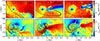 |
Fig. 9. Slices of the gas entropy (top) and velocity in the x − y plane (bottom) from the simulations (ξ0, P0) = (5, 1.5 Mpc), (5, 2.5 Mpc), and (10, 2.5 Mpc) from left to right at t = 3.1, 3.2, 5.0 Gyr, respectively. All slices are taken through the merger plane (the x − y plane). Subcluster trajectories in each simulation are shown by points connected with lines in the top panels, traced from snapshots at 0.1 Gyr intervals. The black vectors in the bottom panels illustrate both direction and amplitude of the velocity field in the merger plane (within ≃600 kpc). The white arrows indicate the LOS directions (projected in the x − y plane) adopted in Fig. 10. The merger with the smallest subhalo and largest impact parameter produces the most regular, least turbulent sloshing spirals in the cluster core (see Sect. 5). |
Arrows in the bottom panels of Fig. 9 show the velocity fields in the merger plane. In all cases, the gas core rotates counterclockwise, following the trajectory of the subhalo as it penetrates the main cluster. The merger with ξ = 10 produces the most regular and least turbulent sloshing pattern, while more massive subhalos drive higher rotational velocities owing to their stronger gravitational perturbations. Despite the sparse sampling, our XRISM measurements reveal a dipole-like bulk-velocity pattern along the east–west direction with an amplitude of approximately ±200 − 300 km s−1 (see Fig. 3). It provides a constraint on the system’s viewing direction. An inclination angle of ≃30° −50°, defined as the angle between the LOS and z-axis in the simulation, is required, with a mild dependence on the merger mass ratio.
Figure 10 shows our modeled projections with snapshots and viewing angles selected to match (1) the bulk velocity distribution and (2) the location of the subhalo as identified in Churazov et al. (2026, top panels) and HyeongHan et al. (2025, bottom panels), respectively. Both simulations reproduce the asymmetric dipole-like velocity pattern. We did not include XRISM/Resolve’s instrumental effects in the modeling, as they are not important for comparisons on ∼100 kpc scales. The top panels, modeling the merger scenario suggested in Churazov et al. (2026) with an inclination angle of i ≃ 40°, resemble major observational features within ∼400 kpc. The subhalo’s trajectory is similar to that indicated by the long radio tail of IC310 (van Weeren et al. 2024), and its LOS velocity (≃300 km s−1) is consistent with the peculiar velocity of the galaxy. However, the velocity dispersion in the outer regions (around R ≃ 200 − 400 kpc) is only ∼100 − 200 km s−1, lower than the measurements from N+NE and O3. A direct comparison of the ulos − σlos space distribution between our observation and merger simulation is shown in Fig. 11. A slightly bigger subhalo (e.g., ξ ∼ 5 − 10) partially alleviates this discrepancy (see the bottom panels). The cosmological environment of Perseus, together with its complex merger history is also, however, likely to contribute to this mismatch, which cannot be captured by our idealized single-merger simulations.
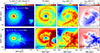 |
Fig. 10. Simulated X-ray surface brightness (0.5 − 8 keV), X-ray-weighted temperature, LOS velocity dispersion, and bulk velocity for simulations with (ξ0, P0) = (10, 2.5 Mpc) and (5, 2.5 Mpc) at t = 5.0 and 3.2 Gyr, viewed at inclination angles i ≃ 40°, respectively. Black contours in the left panels mark the total mass distribution. The models in the top and bottom panels resemble the subcluster perturbers associated with IC310 and NGC1264, which drive the inner sloshing spiral in Perseus, respectively. Both simulations reproduce the asymmetric dipole-like structure in the bulk velocity (see Sect. 5). |
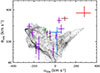 |
Fig. 11. Comparison of the LOS bulk velocity – velocity dispersion space distribution between XRISM observations and the simulation with (ξ0, P0) = (10, 2.5 Mpc) shown in the top panels of Fig. 10. Black dots mark measurements from a uniform grid within R = 400 kpc in the simulation. Observational data are the same as in Fig. 4, but only 1σ errors are shown. Our single-merger simulation reproduces the overall velocity pattern but fails to capture the high-velocity dispersions observed in certain outer regions of the cluster (see Sect. 5). |
We further examined the possibility that NGC1264 and its associated subhalo are responsible for the recent sloshing in Perseus, as proposed by HyeongHan et al. (2025). While we slightly relaxed the merger mass ratio inferred from weak-lensing measurements (i.e., ξ ∼ 3), a value of ξ = 5 remains consistent within the observational uncertainties. Nevertheless, this scenario still faces two major issues that cannot be reconciled. First, a significant fraction of the subhalo’s gas atmosphere is expected to survive after the primary apocentric passage, as shown in the bottom panels of Fig. 10. Its absence in X-ray observations implies a lower gas fraction (or even a gasless case) for the survived subhalo. Second, the peculiar velocity of NGC1264 in Perseus is ∼ − 1800 km s−1, comparable to the total subhalo velocity in our simulation (see Fig. 9). Reproducing such a high LOS velocity would require a sightline that is nearly aligned with the subhalo’s infall direction, which contradicts the dipole-like structure (its orientation) of the ICM bulk velocity. In the projection shown in the bottom panels of Fig. 10, the subhalo’s LOS velocity is only ∼ − 500 km s−1. It is therefore unlikely that the subhalo identified in weak-lensing measurements is the perturber of the sloshing within ∼400 kpc in Perseus. However, it could be a remnant of a previous merger that has undergone multiple orbits and lost most of its gas content and be responsible for the eastern X-ray excess and/or the outer cold front at ∼700 kpc.
Taken together, we suggest that the observed features in Perseus were shaped by at least two mergers. The most recent, ∼3 − 5 Gyr ago, produced the spiral structures within ∼400 kpc, with the subhalo (likely IC310) having recently passed its primary apocenter. The cold front at R ≃ 700 kpc was instead generated by an earlier merger, ∼6 − 9 Gyr before, as inferred from the expansion rate of the sloshing arm (Bellomi et al. 2024). Interestingly, Zhang et al. (2020b) showed that a merger shock formed ∼8 Gyr ago (around redshift z ∼ 1) would be able to explain the giant contact discontinuity found near the virial radius (∼1.7 Mpc) of Perseus (Walker et al. 2022) through a collision between merger and accretion shocks (Zhang et al. 2020a), which may correspond to the same event that produced the R ∼ 700 kpc cold front.
We also note that in both models shown in Fig. 10, the LOS velocity dispersions remain consistently below ≃100 km s−1 within the very central regions (≲60 kpc), significantly lower than the observational measurements (≃200 km s−1; see Fig. 3 and XRISM Collaboration 2025e). This suggests that a single merger alone cannot account for the central peak of the velocity dispersion in Perseus, in line with the argument in XRISM Collaboration (2025e) that AGN feedback plays a crucial role in boosting the observed velocity dispersion at the center.
6. Conclusions
We present extended, up-to-date gas kinematic maps of the Perseus cluster by combining five new XRISM/Resolve pointings observed in 2025 with the PV data from 2024 (XRISM Collaboration 2025e). These observations cover multiple radial directions (i.e., E+NE, S, NW) and a broad range of dynamical scales (∼50 − 500 kpc). To date, Perseus remains the only cluster that has been extensively mapped with a microcalorimeter and high spectral resolution out to ≃0.7r2500 (along multiple radial directions), while simultaneously offering sufficient spatial resolution to resolve gaseous substructures. This unique dataset makes it possible to carry out an unprecedented exploration of the merger-driven gas kinematics in the ICM and provides valuable insights into the merger history of the system. Our main findings are summarized below.
-
We measured high-velocity dispersions (≃300 km s−1) in the east of the cluster (see Fig. 3), spatially coinciding with the extended X-ray surface brightness excess seen in the high-resolution images. These velocities correspond to a nonthermal pressure fraction of ≃7 − 14%, in agreement with the numerical predictions of the Perseus-like clusters in the TNG-Cluster cosmological simulation. In contrast, the fractions in all other (non-AGN-dominant) regions remain consistently below 5%, lower than the TNG-Cluster predictions but comparable to those seen in the most relaxed clusters in TNG300 simulation suite (see Sect. 4.1). We note that anisotropies in the velocity field and X-ray emissivity could potentially complicate the characterization of fnth.
-
We characterized the velocity maps in the non-AGN-dominant region (≳60 kpc) using the second-order velocity structure function and the radial profile of the turbulent heating rate. The observed velocity distributions can be effectively described by a field driven by a single, large-scale kinematic source. This interpretation is supported by both the shape of the velocity structure function and the approximately uniform turbulent heating rate within R ≃ 60 − 400 kpc. Our measurements favor an energy injection scale of at least a few hundred kpc (see Sects. 4.2 and 4.3).
-
An asymmetric dipole-like pattern along the east-west direction, with an amplitude of approximately ±200 − 300 km s−1, is observed in the bulk velocity distribution (see Fig. 3), indicating moderate gas rotation produced by the recent merger process. The E+NE regions correspond to the receding (most positive) side, while the NW arm corresponds to the approaching (most negative) side. This feature provides a strong constraint on the LOS direction, namely, an inclination angle of ≃30° −50°, with a mild dependence on the merger mass ratio.
-
Our idealized merger simulations suggest that Perseus has undergone at least two energetic mergers since redshift z ∼ 1. The more recent event was an off-axis, minor merger with a mass ratio of ∼5 − 10, which occurred ∼3 − 5 Gyr ago and produced the inner spiral structure (≲400 kpc). The remnant of the infalling subcluster has recently passed its primary apocenter, likely corresponding to the radio galaxy IC310. An earlier merger, ∼6 − 9 Gyr ago, generated the ancient cold front at ∼700 kpc. The remnant of that subcluster may correspond to the “gasless” substructure revealed by the weak-lensing measurements (see Sect. 5).
This work demonstrates the power of high-resolution, non-dispersive imaging spectroscopy for probing ICM kinematics and advancing our understanding of cluster dynamics. It paves the way for future projects or missions dedicated to mapping the ICM (e.g., XRISM key projects, HUBS, and NewAthena). Nevertheless, we emphasize that the current sparse velocity coverage limits the statistical significance of our results. Additional XRISM/Resolve observations with a more uniform spatial coverage will be crucial to validate our conclusions.
Acknowledgments
CZ and NW were supported by the GACR EXPRO grant No. 21-13491X. CZ and IZ were partially supported by NASA grant 80NSSC18K1684. CZ, IZ, and AH acknowledge partial support from the Alfred P. Sloan Foundation through the Sloan Research Fellowship. EM acknowledges support from NASA grants 80NSSC20K0737 and 80NSSC24K0678. SU acknowledges support by Program for Forming Japan’s Peak Research Universities (J-PEAKS) Grant Number JPJS00420230006. This work was supported by JSPS KAKENHI grant numbers JP25K23398 (SU). Part of this work was performed under the auspices of the U.S. Department of Energy by Lawrence Livermore National Laboratory under Contract DE-AC52-07NA27344. The material is based upon work supported by NASA under award number 80GSFC24M0006. The simulations presented in this paper were carried out using the Midway computing cluster provided by the University of Chicago Research Computing Center. The software used in this work was developed in part by the DOE NNSA- and DOE Office of Science supported Flash Center for Computational Science at the University of Chicago and the University of Rochester.
References
- Bellomi, E., ZuHone, J. A., Weinberger, R., et al. 2024, ApJ, 974, 234 [NASA ADS] [CrossRef] [Google Scholar]
- Benson, A. J. 2005, MNRAS, 358, 551 [Google Scholar]
- Burkert, A. 1995, ApJ, 447, L25 [NASA ADS] [Google Scholar]
- Canning, R. E. A., Ryon, J. E., Gallagher, J. S., et al. 2014, MNRAS, 444, 336 [CrossRef] [Google Scholar]
- Churazov, E., Forman, W., Jones, C., et al. 2003, ApJ, 590, 225 [NASA ADS] [CrossRef] [Google Scholar]
- Churazov, E., Khabibullin, I., Lyskova, N., et al. 2026, A&A, in press, https://doi.org/10.1051/0004-6361/202556614 [Google Scholar]
- Cruise, M., Guainazzi, M., Aird, J., et al. 2025, Nat. Astron., 9, 36 [Google Scholar]
- Cui, W., Chen, L.-B., Gao, B., et al. 2020, J. Low Temp. Phys., 199, 502 [NASA ADS] [CrossRef] [Google Scholar]
- Cuillandre, J.-C., Bolzonella, M., Boselli, A., et al. 2025, A&A, 697, A11 [Google Scholar]
- de Vries, M., Mantz, A. B., Allen, S. W., et al. 2023, MNRAS, 518, 2954 [Google Scholar]
- Dolag, K., & Sunyaev, R. 2013, MNRAS, 432, 1600 [NASA ADS] [CrossRef] [Google Scholar]
- Evrard, A. E. 1990, ApJ, 363, 349 [NASA ADS] [CrossRef] [Google Scholar]
- Ewart, R. J., Reichherzer, P., Bott, A. F. A., et al. 2024, MNRAS, 532, 2098 [Google Scholar]
- Fabian, A. C. 2012, ARA&A, 50, 455 [Google Scholar]
- Fabian, A. C., Sanders, J. S., Ettori, S., et al. 2000, MNRAS, 318, L65 [Google Scholar]
- Federrath, C., Roman-Duval, J., Klessen, R. S., et al. 2010, A&A, 512, A81 [NASA ADS] [CrossRef] [EDP Sciences] [Google Scholar]
- Forman, W., Kellogg, E., Gursky, H., et al. 1972, ApJ, 178, 309 [Google Scholar]
- Fryxell, B., Olson, K., Ricker, P., et al. 2000, ApJS, 131, 273 [Google Scholar]
- Fujita, Y., Fukushima, K., Sato, K., et al. 2025, PASJ, 77, S270 [Google Scholar]
- Furusho, T., Yamasaki, N. Y., Ohashi, T., et al. 2001, ApJ, 561, L165 [Google Scholar]
- Gatuzz, E., Mohapatra, R., Federrath, C., et al. 2023, MNRAS, 524, 2945 [NASA ADS] [CrossRef] [Google Scholar]
- Gendron-Marsolais, M., Hlavacek-Larrondo, J., van Weeren, R. J., et al. 2020, MNRAS, 499, 5791 [NASA ADS] [CrossRef] [Google Scholar]
- Gilfanov, M. R., Syunyaev, R. A., & Churazov, E. M. 1987, Sov. Astron. Lett., 13, 3 [NASA ADS] [Google Scholar]
- Hitomi Collaboration 2016, Nature, 535, 117 [CrossRef] [Google Scholar]
- Hitomi Collaboration (Aharonian, F., et al.) 2018, PASJ, 70, 9 [NASA ADS] [Google Scholar]
- Hosking, D. N., & Schekochihin, A. A. 2022, JFM, 973, A13 [Google Scholar]
- Hu, Y., Lazarian, A., Brunetti, G., et al. 2025, ApJ, 990, 226 [Google Scholar]
- HyeongHan, K., Jee, M. J., Lee, W., et al. 2025, Nat. Astron., 9, 925 [Google Scholar]
- Ishisaki, Y., Kelley, R. L., Awaki, H., et al. 2022, Proc. SPIE, 12181, 121811S [NASA ADS] [Google Scholar]
- Kang, W., Hwang, H. S., Song, H., et al. 2024, ApJS, 272, 22 [Google Scholar]
- Kitayama, T., Bautz, M., Markevitch, M., et al. 2014, arXiv e-prints [arXiv:1412.1176] [Google Scholar]
- Kolmogorov, A. 1941, Akademiia Nauk SSSR Doklady, 30, 301 [Google Scholar]
- Kraft, R., Markevitch, M., Kilbourne, C., et al. 2022, arXiv e-prints [arXiv:2211.09827] [Google Scholar]
- Lau, E. T., Kravtsov, A. V., & Nagai, D. 2009, ApJ, 705, 1129 [NASA ADS] [CrossRef] [Google Scholar]
- Li, Y., & Bryan, G. L. 2014, ApJ, 789, 54 [NASA ADS] [CrossRef] [Google Scholar]
- Lodders, K., Palme, H., & Gail, H.-P. 2009, Landolt Börnstein, 4B, 712 [Google Scholar]
- Marinacci, F., Vogelsberger, M., Pakmor, R., et al. 2018, MNRAS, 480, 5113 [NASA ADS] [Google Scholar]
- Markevitch, M., & Vikhlinin, A. 2007, Phys. Rep., 443, 1 [Google Scholar]
- Miniati, F. 2014, ApJ, 782, 21 [NASA ADS] [CrossRef] [Google Scholar]
- Miniati, F., & Beresnyak, A. 2015, Nature, 523, 59 [NASA ADS] [CrossRef] [Google Scholar]
- Nagai, D., Vikhlinin, A., & Kravtsov, A. V. 2007, ApJ, 655, 98 [Google Scholar]
- Nagai, H., Onishi, K., Kawakatu, N., et al. 2019, ApJ, 883, 193 [NASA ADS] [CrossRef] [Google Scholar]
- Naiman, J. P., Pillepich, A., Springel, V., et al. 2018, MNRAS, 477, 1206 [Google Scholar]
- Navarro, J. F., Frenk, C. S., & White, S. D. M. 1997, ApJ, 490, 493 [Google Scholar]
- Nelson, D., Pillepich, A., Springel, V., et al. 2018, MNRAS, 475, 624 [Google Scholar]
- Nelson, D., Springel, V., Pillepich, A., et al. 2019, Comput. Astrophys. Cosmol., 6, 2 [Google Scholar]
- Nelson, D., Pillepich, A., Ayromlou, M., et al. 2024, A&A, 686, A157 [NASA ADS] [CrossRef] [EDP Sciences] [Google Scholar]
- Norman, M. L., & Bryan, G. L. 1999, Radio Galaxy Messier, 87, 106 [Google Scholar]
- Pillepich, A., Nelson, D., Hernquist, L., et al. 2018, MNRAS, 475, 648 [Google Scholar]
- Poole, G. B., Fardal, M. A., Babul, A., et al. 2006, MNRAS, 373, 881 [Google Scholar]
- Porter, F. S., Kilbourne, C. A., Chiao, M., et al. 2024, Proc. SPIE, 13093, 130931K [Google Scholar]
- Reynolds, C. S., McKernan, B., Fabian, A. C., et al. 2005, MNRAS, 357, 242 [NASA ADS] [CrossRef] [Google Scholar]
- Salomé, P., Combes, F., Edge, A. C., et al. 2006, A&A, 454, 437 [CrossRef] [EDP Sciences] [Google Scholar]
- Sanders, J. S., Dennerl, K., Russell, H. R., et al. 2020, A&A, 633, A42 [EDP Sciences] [Google Scholar]
- Schwarz, R. A., Edge, A. C., Voges, W., et al. 1992, A&A, 256, L11 [NASA ADS] [Google Scholar]
- Shi, X., & Komatsu, E. 2014, MNRAS, 442, 521 [NASA ADS] [CrossRef] [Google Scholar]
- Shi, X., & Zhang, C. 2019, MNRAS, 487, 1072 [NASA ADS] [CrossRef] [Google Scholar]
- Shi, X., Nagai, D., Aung, H., et al. 2020, MNRAS, 495, 784 [NASA ADS] [CrossRef] [Google Scholar]
- Simionescu, A., Werner, N., Urban, O., et al. 2012, ApJ, 757, 182 [CrossRef] [Google Scholar]
- Simionescu, A., ZuHone, J., Zhuravleva, I., et al. 2019, Space Sci. Rev., 215, 24 [NASA ADS] [CrossRef] [Google Scholar]
- Sohn, J., Geller, M. J., Walker, S. A., et al. 2019, ApJ, 871, 129 [NASA ADS] [CrossRef] [Google Scholar]
- Springel, V. 2010, MNRAS, 401, 791 [Google Scholar]
- Springel, V., Pakmor, R., Pillepich, A., et al. 2018, MNRAS, 475, 676 [Google Scholar]
- Subramanian, K., Shukurov, A., & Haugen, N. E. L. 2006, MNRAS, 366, 1437 [CrossRef] [Google Scholar]
- Tang, X., & Churazov, E. 2017, MNRAS, 468, 3516 [Google Scholar]
- Tashiro, M., Maejima, H., Toda, K., et al. 2021, Proc. SPIE, 11444, 1144422 [Google Scholar]
- Timmerman, R., van Weeren, R. J., Botteon, A., et al. 2022, A&A, 668, A65 [NASA ADS] [CrossRef] [EDP Sciences] [Google Scholar]
- Truong, N., Pillepich, A., Nelson, D., et al. 2024, A&A, 686, A200 [NASA ADS] [CrossRef] [EDP Sciences] [Google Scholar]
- Ueda, S., Hayashida, K., Nakajima, H., et al. 2013, Astronom. Nachr., 334, 426 [Google Scholar]
- van Weeren, R. J., Timmerman, R., Vaidya, V., et al. 2024, A&A, 692, A12 [NASA ADS] [CrossRef] [EDP Sciences] [Google Scholar]
- Vazza, F., & Brunetti, G. 2026, A&A, 705, A129 [NASA ADS] [CrossRef] [EDP Sciences] [Google Scholar]
- Vazza, F., Brunetti, G., Kritsuk, A., et al. 2009, A&A, 504, 33 [NASA ADS] [CrossRef] [EDP Sciences] [Google Scholar]
- Vazza, F., Brunetti, G., Gheller, C., et al. 2011, A&A, 529, A17 [NASA ADS] [CrossRef] [EDP Sciences] [Google Scholar]
- Vitvitska, M., Klypin, A. A., Kravtsov, A. V., et al. 2002, ApJ, 581, 799 [NASA ADS] [CrossRef] [Google Scholar]
- Walker, S. A., ZuHone, J., Fabian, A., et al. 2018, Nat. Astron., 2, 292 [NASA ADS] [CrossRef] [Google Scholar]
- Walker, S. A., Mirakhor, M. S., ZuHone, J., et al. 2022, ApJ, 929, 37 [NASA ADS] [CrossRef] [Google Scholar]
- Weinberger, R., Springel, V., & Pakmor, R. 2020, ApJS, 248, 32 [Google Scholar]
- Werner, N., Urban, O., Simionescu, A., et al. 2013, Nature, 502, 656 [Google Scholar]
- Willingale, R., Starling, R. L. C., Beardmore, A. P., et al. 2013, MNRAS, 431, 394 [NASA ADS] [CrossRef] [Google Scholar]
- XRISM Collaboration 2025a, ApJ, 982, L5 [Google Scholar]
- XRISM Collaboration 2025b, PASJ, 77, S242 [Google Scholar]
- XRISM Collaboration 2025c, Nature, 638, 365 [Google Scholar]
- XRISM Collaboration 2025d, ApJ, 985, L20 [Google Scholar]
- XRISM Collaboration 2025e, arXiv e-prints [arXiv:2509.04421] [Google Scholar]
- XRISM Collaboration 2025f, ApJ, 993, L11 [Google Scholar]
- Zhang, C., Yu, Q., & Lu, Y. 2014, ApJ, 796, 138 [NASA ADS] [CrossRef] [Google Scholar]
- Zhang, C., Yu, Q., & Lu, Y. 2015, ApJ, 813, 129 [NASA ADS] [CrossRef] [Google Scholar]
- Zhang, C., Churazov, E., Dolag, K., et al. 2020a, MNRAS, 494, 4539 [NASA ADS] [CrossRef] [Google Scholar]
- Zhang, C., Churazov, E., Dolag, K., et al. 2020b, MNRAS, 498, L130 [NASA ADS] [CrossRef] [Google Scholar]
- Zhang, C., Zhuravleva, I., Gendron-Marsolais, M.-L., et al. 2022, MNRAS, 517, 616 [CrossRef] [Google Scholar]
- Zhang, C., Zhuravleva, I., Markevitch, M., et al. 2024, MNRAS, 530, 4234 [NASA ADS] [CrossRef] [Google Scholar]
- Zhuravleva, I., Churazov, E., Kravtsov, A., et al. 2012, MNRAS, 422, 2712 [NASA ADS] [CrossRef] [Google Scholar]
- Zhuravleva, I., Churazov, E., Schekochihin, A. A., et al. 2014, Nature, 515, 85 [Google Scholar]
- Zhuravleva, I., Churazov, E., Arévalo, P., et al. 2015, MNRAS, 450, 4184 [NASA ADS] [CrossRef] [Google Scholar]
- Zuhone, J. A., & Roediger, E. 2016, J. Plasma Phys., 82, 535820301 [CrossRef] [Google Scholar]
- ZuHone, J. A., Markevitch, M., Brunetti, G., et al. 2013, ApJ, 762, 78 [NASA ADS] [CrossRef] [Google Scholar]
- ZuHone, J. A., Markevitch, M., & Zhuravleva, I. 2016, ApJ, 817, 110 [NASA ADS] [CrossRef] [Google Scholar]
As of the preparation of this paper, the C3 pointing has also been completed. An in-depth joint analysis between the full NW and S arms will be presented in a companion paper, featuring gas velocities within the Perseus cool core.
The rΔ represents the radius within which an average mass density is Δ (e.g. 2500, 500, 200) times the critical density of the Universe at the cluster redshift.
A detailed numerical modeling study of A2029 will be presented in a separate paper.
Appendix A: Supplementary observational details
A.1. New XRISM pointings
We included five new pointings observed after the XRISM PV phase in our analysis. Their observation IDs and pointing coordinates are listed in Table A.1. The O3 pointing was observed in July 2025 with a heliocentric correction of ≃24 km s−1 and the rest four were observed in January-February 2025 with heliocentric corrections of ≃ − 28 − −25 km s−1.
Additional information about the calibration/GO pointings.
A.2. Radial profile of the Fe abundance
Figure A.1 shows the radial profile of the Fe abundance, the most extended measurements by XRISM/Resolve to date, alongside those for A2029 (XRISM Collaboration 2025b). We emphasize that the central bright AGN and imperfect PSF calibration may introduce significant systematic uncertainties for the inner sub-regions (≲60kpc), preventing us from firmly concluding whether an abundance drop exists in the center. For reference, we show also the full-FOV fit of the PV data with SSM correction (XRISM Collaboration 2025e). The profile flattens at ∼150kpc, generally consistent with previous XMM-Newton and Suzaku measurements (e.g., Churazov et al. 2003; Ueda et al. 2013; Werner et al. 2013).
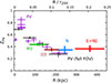 |
Fig. A.1. Radial profile of the Fe abundance, using the same color scheme as in Fig. 4. Black points show the results from PV pointings, full-FOV fit (XRISM Collaboration 2025e). |
A.3. X-ray emissivity effective length
We followed XRISM Collaboration (2025e) to estimate the effective length ℓeff, defined as the region size that contributes 50% of the flux to the total flux at each projected distance from the cluster center. The uncertainties are characterized by varying the contributing fraction by ±10% (shown as the shaded regions in Fig. A.2). The Perseus cluster (grey) and A2029 (yellow) exhibit comparable effective length radial profiles.
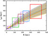 |
Fig. A.2. Effective length radial profiles in Perseus (grey) and A2029 (yellow). The shaded bands indicate the scales contributing 40 − 60% of the flux, which are adopted as the uncertainties in our ℓeff estimates. The boxes mark the scale ranges covered by our regions in Perseus (color scheme as in Fig. 4; see also Table 1). |
A.4. A joint fitting between the E and NE pointings
Figure A.3 compares the velocities measured individually from the E and NE pointings with those obtained from their joint fitting (E+NE), assuming a single-temperature model. They all exhibit consistent bulk velocities and velocity dispersions. In the joint fit, all parameters except the normalization are tied between the models for the E and NE spectra.
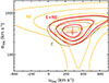 |
Fig. A.3. Same as Fig. 4 but for the E and NE pointings modeled separately (orange and gray contours). The combined fit (red), included for the comparison, is the same as in Fig. 4. |
A.5. Multiple components in the region E
A ∼2 − 3σ deviation between the best-fit 1T model and the Fe Lyα lines hints the presence of an additional hotter component in the region E (see Fig. 2), which dominates the Fe Lyα lines and is redshifted relative to the other, colder component. To explore this in more detail, we fitted the spectrum with two bvapec components, neglecting resonance scattering effects, as no reasonable fit could otherwise be obtained. The top panel of Fig. A.4 shows the best-fit 2T model along with its two individual ICM components: the hot and cold dominating the Fe Lyα and Heα line fluxes, respectively (see also Fig. 2 for a zoom-in near 6.7keV). Their relative velocity is ≃540 ± 100km s−1. The temperature and velocity dispersion of the hot component cannot be tightly constrained. The bottom panel of Fig. A.4 shows the parameter space of the hot component’s temperature vs. the cold component’s velocity dispersion, where colors show the Δ-statistic in units of σ. The velocity dispersion of the cold component (the dominant one) mildly depends on the temperature of the hot component. There are still large uncertainties in this 2T fit, limited by the quality of the current data. Deeper observations of the region are required to confirm the results.
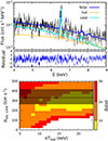 |
Fig. A.4. Top panels: Spectrum in the region E with the best-fit 2T model (blue). The cyan and yellow lines show its cold and hot ICM components, respectively. Bottom panel:Δ-statistic map in the 2D parameter space: the hot component’s temperature vs. the cold component’s velocity dispersion. The color indicates the 1, 2, and 3σ regions. The hot component cannot be tightly constrained in our fittings. |
A.6. The lremover model in Xspec
Instead of manually modifying the atomic database (e.g., Hitomi Collaboration 2018), we used the lremover model4 to remove the Fe Heα resonance line (w-line) from the bvapec model in Xspec and replaced it with an external Gaussian component to account for the resonance scattering effect (e.g., Gilfanov et al. 1987). The main idea of the model is to introduce a negative Gaussian line that cancels the w-line (or any other specified line or lines) in bvapec. Figure A.5 shows an example of the best-fit model, bvapec+lremover+gauss, for the central pointing of Perseus. The same model was employed in XRISM Collaboration (2025e).
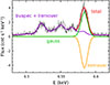 |
Fig. A.5. An example of using the lremover model to remove the Fe Heαw-line from the bvapec model. The model generates a negative Gaussian line that exactly cancels the w-line in bvapec. |
Appendix B: Simulation methods
We performed two types of numerical simulations to support theoretical interpretation of the measured gas kinematic fields, including (1) turbulent simulations using the mesh-based magnetohydrodynamic code FLASH4.6 (Fryxell et al. 2000) and (2) idealized cluster merger simulations using the moving-mesh code AREPO (Springel 2010; Weinberger et al. 2020).
B.1. Turbulent simulations
The turbulent simulations are similar to those presented in XRISM Collaboration (2025e). Turbulence was driven in a Perseus-like cluster by a stochastic forcing term based on the Ornstein-Uhlenbeck process (see Federrath et al. 2010, and references therein), where we included only the solenoidal stirring mode, which dominates in galaxy clusters. The simulation domain is a cube of 1.2Mpc with a spatial resolution of 5kpc, sufficient for the purpose of our experiments. We explored various injection scales ℓinj = 0.2, 0.5, and 1Mpc. Figure B.1 compares the Gaussian random field and the turbulent simulation, both with ℓinj = 1Mpc. The shape and scatter range of their velocity structure functions are very similar, despite the presence of gravitational stratification in the simulations. We note that, although the amplitude of the velocity fields can be fine-tuned in our numerical model, it cannot be arbitrarily high because the simulation does not include radiative cooling. Excessive turbulent heating would rapidly redistribute the gas atmosphere, explaining the underestimate of the velocity structure function in our simulations. However, this is not in tension with the observations. The numerical set-ups assume a spatially and temporarily uniform heating rate, which is unlikely the case in actual clusters.
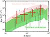 |
Fig. B.1. Comparison of the velocity structure function from the Gaussian random field and the turbulent simulation, both with ℓinj = 1Mpc. The observational data are identical to those in Fig. 6. |
B.2. Merger simulations
In our merger simulations, we modeled mergers between two idealized galaxy clusters. Each cluster consists of both gas and DM halo components, which are spherical and in equilibrium in their initial conditions (see Zhang et al. 2014, 2015 for more details on our numerical set-ups).
The initial DM density radial profile within the virial radius follows the Navarro–Frenk–White form Navarro et al. (1997) and the concentration parameter is fixed to 4 for all halos in our simulations, motivated by recent weak-lensing measurements (HyeongHan et al. 2025). The gas density radial profile of the main cluster is tailored for Perseus, following the Eq. F3 in Tang & Churazov (2017). We adjusted its density normalization to ensure that the averaged gas fraction within the virial radius is fgas = 0.12. The radial temperature profile is determined by the hydrostatic equilibrium condition, which exhibits a ∼100kpc cool core consistent with the observations (Churazov et al. 2003). For the smaller subcluster, its density radial profile is assumed as the Burkert profile (Burkert 1995) with an averaged gas fraction fgas = 0.12.
We fixed the mass of the main cluster (M0 = 6 × 10¹⁴ M⊙) in all our simulations, along with the initial pairwise velocity ( ) between the two merging clusters, based on an empirical relation from cosmological simulations (Dolag & Sunyaev 2013). We explored other parameters that determine the merging halo trajectories, including the merger mass ratio (ξ0 = 5 and 10) and impact parameter (P0 = 1.5, 2.5, 3.5 Mpc). The mergers are set to occur in the x − y plane (i.e., the merger plane), with the initial cluster velocities aligned along the y-axis (see Fig. 9). The mass resolutions of the DM and gas are ≃5 × 10⁸ and 2 × 10⁷ M⊙, respectively.
All Tables
All Figures
|
Fig. 1. XRISM/Resolve pointings used in this work, labeled with their region names. The background shows the XMM-Newton X-ray surface brightness in the 0.5 − 3.5 keV band (Churazov et al. 2026). White arrows indicate the sloshing cold fronts identified in the system (e.g., Walker et al. 2018). The pointings E, NE, and N (calibration), together with M3 and O3 (GO cycle 1 observations), are newly reported in this work, marked in yellow (see Sect. 2). |
| In the text | |
|
Fig. 2. Fe Heα and Lyα lines in the E region with best-fit 1T and 2T models. The spectrum suggests the presence of an additional, more redshifted, hotter component, which would have to be confirmed with deeper observations. Residuals normalized by the statistical errors, i.e., (data-model)/error, are displayed in the lower panel (see Sect. 2 and Appendix A.5). |
| In the text | |
|
Fig. 3. Best-fit gas bulk velocity (left) and velocity dispersion (right) maps of the Perseus cluster from nine XRISM/Resolve pointings. The maps are centered on the Perseus center (RA = 49.9507, Dec = 41.5117). The N and NE regions show the E+NE joint fitting result assuming a single temperature model. The color patches indicate the sky areas that contribute 50% of the photons for the corresponding sub-regions based on raytracing simulations. The measurement uncertainties are shown in Fig. 4. The Chandra X-ray residual is overlaid in the background highlighting the inner sloshing spiral and the eastern X-ray surface brightness excess, with black circles marking radii of 100, 200, and 300 kpc. The bulk velocity distribution, in the rest frame of the central ICM (zicm = 0.017628), shows an (asymmetric) dipole-like pattern, revealing a rotational motion of the ICM (see Sect. 3). |
| In the text | |
|
Fig. 4. 2D confidence contours (1, 2, and 3σ) of the bulk velocity and velocity dispersion measurements of our new regions (calibration and GO pointings). The red contours indicate a joint fit between the E and NE regions (see Fig. A.3 for their individual fits). The crosses mark the best-fit parameters and their 1σ uncertainties, including also all PV data (ten sub-regions; see Sect. 3). The pink cross indicates the cold ICM component in the 2T model for region E (see Sect. 2). |
| In the text | |
|
Fig. 5. Nonthermal pressure fraction profile of the Perseus cluster, compared with A2029 (grey points; XRISM Collaboration 2025b). Colors follow the same scheme as in Fig. 4 for Perseus. The shaded bands show numerical predictions from TNG cosmological simulations for two cluster subsamples: (i) the 31 most relaxed clusters from the TNG-300 simulation suite (yellow) and (ii) 30 Perseus-like massive, cool-core clusters from TNG-Cluster suite (pink). The bands represent the 10th-90th percentile range of the fnth distribution within each sample. The inner AGN-dominant region, as well as the regions overlapping the eastern X-ray surface brightness excess (E+NE and O3), show high fnth (> 7%; see Sect. 4.1). |
| In the text | |
|
Fig. 6. Second-order velocity structure function for the velocity field outside the AGN-dominant region (≳60 kpc) in Perseus, grouped into four bins (red points). Black points show all available velocity pairs with their 1σ statistical uncertainties. The shaded regions show theoretical predictions and their 68% scatters based on Gaussian random fields. Various energy injection scales (top) and spectral indices are shown to compare with the observations. The XRISM Perseus dataset favors a large injection scale (at least a few hundred kpc) but is not sensitive to the spectral index (see Sect. 4.2). |
| In the text | |
|
Fig. 7. Effect of X-ray emissivity distribution on modulating the dominant velocity power spectrum we probe. The X-ray emissivity acts as a velocity high-pass filter, allowing us to probe only the largest scales smaller than 1/ℓeff in k-space (see Appendix A.3 for definition and calculation of ℓeff). The pink regions depict the range of spatial scales that dominate the gas kinematic energy in the measurements. In this work, we focus on merger-driven, large-scale gas motions, which are likely to correspond to the situation shown on the left (see Sect. 4.3). |
| In the text | |
|
Fig. 8. Radial profile of the turbulent heating rate. The color scheme is the same as in Fig. 4. The uncertainties incorporate both the velocity statistical errors and effective length variations within each region. Outside the AGN-dominant region (i.e., ≳60 kpc), the heating rate appears approximately uniform (∼10−28 − 10−27 erg cm−3 s−1, marked by the grey band), covering a dynamical range of ℓeff ≃ 100 − 400 kpc (see Sect. 4.3). |
| In the text | |
|
Fig. 9. Slices of the gas entropy (top) and velocity in the x − y plane (bottom) from the simulations (ξ0, P0) = (5, 1.5 Mpc), (5, 2.5 Mpc), and (10, 2.5 Mpc) from left to right at t = 3.1, 3.2, 5.0 Gyr, respectively. All slices are taken through the merger plane (the x − y plane). Subcluster trajectories in each simulation are shown by points connected with lines in the top panels, traced from snapshots at 0.1 Gyr intervals. The black vectors in the bottom panels illustrate both direction and amplitude of the velocity field in the merger plane (within ≃600 kpc). The white arrows indicate the LOS directions (projected in the x − y plane) adopted in Fig. 10. The merger with the smallest subhalo and largest impact parameter produces the most regular, least turbulent sloshing spirals in the cluster core (see Sect. 5). |
| In the text | |
|
Fig. 10. Simulated X-ray surface brightness (0.5 − 8 keV), X-ray-weighted temperature, LOS velocity dispersion, and bulk velocity for simulations with (ξ0, P0) = (10, 2.5 Mpc) and (5, 2.5 Mpc) at t = 5.0 and 3.2 Gyr, viewed at inclination angles i ≃ 40°, respectively. Black contours in the left panels mark the total mass distribution. The models in the top and bottom panels resemble the subcluster perturbers associated with IC310 and NGC1264, which drive the inner sloshing spiral in Perseus, respectively. Both simulations reproduce the asymmetric dipole-like structure in the bulk velocity (see Sect. 5). |
| In the text | |
|
Fig. 11. Comparison of the LOS bulk velocity – velocity dispersion space distribution between XRISM observations and the simulation with (ξ0, P0) = (10, 2.5 Mpc) shown in the top panels of Fig. 10. Black dots mark measurements from a uniform grid within R = 400 kpc in the simulation. Observational data are the same as in Fig. 4, but only 1σ errors are shown. Our single-merger simulation reproduces the overall velocity pattern but fails to capture the high-velocity dispersions observed in certain outer regions of the cluster (see Sect. 5). |
| In the text | |
|
Fig. A.1. Radial profile of the Fe abundance, using the same color scheme as in Fig. 4. Black points show the results from PV pointings, full-FOV fit (XRISM Collaboration 2025e). |
| In the text | |
|
Fig. A.2. Effective length radial profiles in Perseus (grey) and A2029 (yellow). The shaded bands indicate the scales contributing 40 − 60% of the flux, which are adopted as the uncertainties in our ℓeff estimates. The boxes mark the scale ranges covered by our regions in Perseus (color scheme as in Fig. 4; see also Table 1). |
| In the text | |
|
Fig. A.3. Same as Fig. 4 but for the E and NE pointings modeled separately (orange and gray contours). The combined fit (red), included for the comparison, is the same as in Fig. 4. |
| In the text | |
|
Fig. A.4. Top panels: Spectrum in the region E with the best-fit 2T model (blue). The cyan and yellow lines show its cold and hot ICM components, respectively. Bottom panel:Δ-statistic map in the 2D parameter space: the hot component’s temperature vs. the cold component’s velocity dispersion. The color indicates the 1, 2, and 3σ regions. The hot component cannot be tightly constrained in our fittings. |
| In the text | |
|
Fig. A.5. An example of using the lremover model to remove the Fe Heαw-line from the bvapec model. The model generates a negative Gaussian line that exactly cancels the w-line in bvapec. |
| In the text | |
|
Fig. B.1. Comparison of the velocity structure function from the Gaussian random field and the turbulent simulation, both with ℓinj = 1Mpc. The observational data are identical to those in Fig. 6. |
| In the text | |
Current usage metrics show cumulative count of Article Views (full-text article views including HTML views, PDF and ePub downloads, according to the available data) and Abstracts Views on Vision4Press platform.
Data correspond to usage on the plateform after 2015. The current usage metrics is available 48-96 hours after online publication and is updated daily on week days.
Initial download of the metrics may take a while.