| Issue |
A&A
Volume 707, March 2026
|
|
|---|---|---|
| Article Number | A20 | |
| Number of page(s) | 11 | |
| Section | Extragalactic astronomy | |
| DOI | https://doi.org/10.1051/0004-6361/202557780 | |
| Published online | 25 February 2026 | |
The MALATANG survey: Star formation, dense gas, and active galactic nucleus feedback in NGC 1068
1
Department of Astronomy, Xiamen University, Zengcuo’an West Road Xiamen 361005
2
School of Astronomy and Space Science, Nanjing University, Nanjing 210093
3
Key Laboratory of Modern Astronomy and Astrophysics (Nanjing University), Ministry of Education, Nanjing 210093
4
Purple Mountain Observatory, Chinese Academy of Sciences, 10 Yuanhua road Nanjing 210023
5
School of Physical Science and Technology, Guangxi University, Nanning 530004
6
Research Center for Astronomical Computing, Zhejiang Laboratory, Hangzhou 311121
7
Shandong Key Laboratory of Space Environment and Exploration Technology, College of Physics and Electronic Information, Dezhou University, Dezhou 253023
8
Department of Physics, Hebei Normal University (Physics Postdoctoral Research Station at Hebei Normal University), Shijiazhuang 050024
9
Guo Shoujing Institute for Astronomy, Hebei Normal University, Shijiazhuang 050024
10
Hebei Advanced Thin Films Laboratory, Shijiazhuang 050024
11
Institute of Astronomy and Astrophysics, Academia Sinica, 11F of Astro-Math Building, AS/NTU, No.1, Sec. 4, Roosevelt Rd Taipei 10617
12
Department of Astronomy, Yonsei University 50 Yonsei-ro Seodaemun-gu Seoul 03722, Republic of Korea
13
Institute of Astronomy, Graduate School of Science, The University of Tokyo 2-21-1 Osawa Mitaka Tokyo 181-0015, Japan
14
Joetsu University of Education, Yamayashiki-machi Joetsu Niigata 943-8512, Japan
15
Cosmic Dawn Center (DAWN) Copenhagen, Denmark
16
DTU-Space, Technical University of Denmark Elektrovej 327 DK-2800 Kgs. Lyngby, Denmark
17
Department of Physics and Astronomy, University College London Gower Street London WC1E 6BT, UK
★ Corresponding author: This email address is being protected from spambots. You need JavaScript enabled to view it.
Received:
21
October
2025
Accepted:
26
November
2025
Abstract
Aims. We investigated the interplay between dense molecular gas, star formation, and active galactic nucleus (AGN) feedback in the luminous IR galaxy NGC 1068 at sub-kiloparsec scales.
Methods. We present the HCN (4-3) and HCO+ (4-3) maps of NGC 1068 obtained with JCMT as part of the Mapping the dense molecular gas in the strongest star-forming galaxies (MALATANG) project, and perform spatially resolved analyses of their correlations with IR luminosity and soft X-ray emission.
Results. The spatially resolved relations between the luminosities of IR dust emission and dense molecular gas tracers (LIR − L′dense) are found to be nearly linear, without clear evidence of excess contributions from AGN activity. The spatially resolved X-ray emission (Lgas0.5−2 KeV) displays a radially dependent twofold correlation with the star formation rate (SFR), suggesting distinct gas-heating mechanisms are at play in areas between the galaxy center and the outer regions. A super-linear scaling is obtained in galactic center regions with SFR surface densities (ΣSFR) > 8.2 × 10⁻⁶ M⊙ yr−1 kpc−2: log(Lgas0.5−2 KeV/erg s−1) = 2.2 log(SFR/M⊙ yr−1) + 39.1. We further find a statistically significant super-linear correlation (β = 1.34 ± 0.86) between Lgas0.5−2 KeV/SFR and the HCN(4–3)/CO(1–0) intensity ratio, whereas no such trend is seen for HCO+(4-3)/CO(1-0) or CO(3-2)/CO(1-0). These findings indicate that AGN feedback does not dominate star formation regulation on sub-kiloparsec scales, and that the excitation of dense gas traced by HCN (4-3) may be more directly influenced by high-energy feedback processes compared to HCO+ (4-3) and CO (3-2).
Key words: galaxies: ISM / galaxies: individual: NGC 1068 / galaxies: Seyfert / galaxies: star formation
© The Authors 2026
 Open Access article, published by EDP Sciences, under the terms of the Creative Commons Attribution License (https://creativecommons.org/licenses/by/4.0), which permits unrestricted use, distribution, and reproduction in any medium, provided the original work is properly cited.
This article is published in open access under the Subscribe to Open model. This email address is being protected from spambots. You need JavaScript enabled to view it. to support open access publication.
1. Introduction
The process of star formation within galaxies is a key focus of modern astrophysics. Observational studies on galactic scales, using tracers such as Hα, H I, and CO lines, have revealed a power-law relationship between surface densities of the star formation rate (SFR) and the total neutral gas, expressed as  , with an index (N) ≈ 1.4 (Kennicutt 1998; Kennicutt & Evans 2012). This empirical relation is widely known as the Kennicutt–Schmidt (K–S) law. Subsequent studies indicated that stars primarily form from molecular gas (e.g., Bigiel et al. 2008; Liu et al. 2015).
Star formation has been proposed to only occur in molecular regions with densities higher than that of threshold regions in molecular clouds (Av > 8; Lada et al. 2010; Heiderman et al. 2010). On the other hand, the turbulence-regulated model suggests that the formation of stars is governed by the balance between gravitational collapse and the pressure support provided by turbulence within the gas (e.g., Krumholz & McKee 2005; Krumholz & Thompson 2007; Federrath & Klessen 2012; Usero et al. 2015). Observations show that gas tracers with a critical density (ncrit) > 104 cm−3 (e.g., rotational transitions of HCN, HCO+, and CS) exhibit a closer correlation with active star-forming regions than the lower transitions of CO (e.g., Wu et al. 2005; Lada et al. 2010, 2012; Evans et al. 2014; Zhang et al. 2014). In particular, a tight linear correlation between total IR and HCN (1-0) luminosity has been established based on a large sample of local galaxies (Gao & Solomon 2004a,b). This relationship also holds at high redshifts (e.g., Gao et al. 2007) and in individual Galactic clumps (Wu et al. 2005).
With advancements in telescopes, high-resolution imaging of molecular gas has enabled a more detailed understanding of the star formation process and the surrounding physical environments on resolved scales (e.g., Schinnerer et al. 2013; Leroy et al. 2021; Lee et al. 2021). However, the connection between star formation and its physical environment is not fully understood. Several studies report a breakdown of the K–S relation at resolved scales (Onodera et al. 2010; Xu et al. 2015; Nguyen-Luong et al. 2016), possibly due to variations in the evolutionary stages of giant molecular clouds (Onodera et al. 2010). On the one hand, stellar and supernova feedback can significantly influence star formation efficiency by heating gas (Cox et al. 2006; Springel & Hernquist 2005; Choi et al. 2015). Notably, diffuse 2–10 keV X-ray emission from the hot interstellar medium serves as a crucial diagnostic of stellar feedback, exhibiting a super-linear correlation with the SFR in nearby star-forming galaxies (Ranalli et al. 2003; Grimm et al. 2003; Gilfanov et al. 2004; Zhang et al. 2024; Zhang & Wang 2025).
On the other hand, the role of active galactic nucleus (AGN) feedback in regulating star formation remains controversial. While some studies suggest that AGN activity can enhance star formation and boost the SFR (e.g., Santini et al. 2012; Mountrichas et al. 2024), others propose that AGN feedback suppresses star formation by heating or expelling cold gas from the host galaxy, resulting in a lower SFR compared to non-AGN systems (e.g., Shimizu et al. 2015).
Understanding the link between star formation and dense molecular gas with n > 106 cm−3 requires observations of high-J transitions of HCN and HCO+ (Shirley 2015). To bridge the observational gap between Galactic and extragalactic studies of spatially resolved star formation, the Mapping the dense molecular gas in the strongest star-forming galaxies (MALATANG) project was initiated. It is the first systematic survey mapping HCN J = 4 − 3 and HCO+J = 4 − 3 line emissions across 28 nearby IR-bright galaxies using the James Clerk Maxwell Telescope (JCMT). A linear correlation between dense gas luminosity and total IR luminosity on sub-kiloparsec scales was reported by Tan et al. (2018), based on observations of six galaxies from the MALATANG survey.
NGC 1068, one of the targets of the MALATANG project, is a nearby typical Seyfert 2 galaxy at a distance of 15.7 Mpc (1″ = 76 pc; Tan et al. 2018). NGC 1068 is known to host an AGN, which is surrounded by a circumnuclear starburst (SB) ring (Simkin et al. 1980). As one of the nearest and isolated luminous IR galaxies, it has a high global SFR of < 44 M⊙ yr−1 (Howell et al. 2010), which represents an upper limit because of AGN contamination, while the disk SFR is 3.2 M⊙ yr−1 (Nagashima et al. 2024). This makes it an ideal laboratory for investigating how AGN feedback affects dense molecular gas emission and star formation. However, previous studies of dense molecular gas in NGC 1068 (e.g., Schinnerer et al. 2000; Krips et al. 2011; Wang et al. 2014; Sánchez-García et al. 2022; Gámez Rosas et al. 2025) have primarily focused on high-resolution observations of the SB ring and the central circumnuclear disk (CND) within approximately 1 kpc. Investigations of dense gas in the larger galactic disk and spiral arms remain relatively limited.
This paper is organized as follows. In Sect. 2 we describe the observations and data reduction procedures. In Sect. 3 we present the main results, including the integrated-intensity maps and the correlations between line luminosity and IR luminosity, as well as between X-ray luminosity and the SFR. In Sect. 4 we discuss the influence of AGN activity on IR, X-ray, and molecular gas emission, and examine the correlations between dust temperature and molecular line ratios, as well as between the X-ray luminosity/SFR ratio and line ratios. Section 5 summarizes our main conclusions.
2. Observations and data reduction
In this section we present the observations and data reduction of NGC 1068 in the context of the MALATANG project, as well as the ancillary data used in this work. The fundamental properties of NGC 1068 are summarized in Table 1.
Parameters of NGC 1068.
2.1. Observations of HCN (4-3) and HCO+ (4-3)
The HCN (4 − 3) and HCO+ (4 − 3) data of NGC 1068 were obtained from the MALATANG project (program codes: M16AL007 and M20AL022), observed with the Heterodyne Array Receiver Program (HARP) receiver on board the JCMT telescope. HARP has 16 receptors laid out with 4 × 4 grids, and two of them (H13, H14) were nonoperational during the observation. The receiver backend used is an Auto-Correlation Spectral Imaging System (ACSIS) spectrometer. Observations were carried out in jiggle-chop mode, with each receptor jiggled in a 3 × 3 patterns and a beam spacing of 10″. The observation was taken in 2015 and 2016, with total integration times of 250 min for HCN (4 − 3), and 287 min for HCO+ (4 − 3). The full width at half maximum (FWHM) is approximately 14″ at 345 GHz. Further observational details can be found in Tan et al. (2018).
Figure 1 shows the observing positions (marked by orange circles) overlaid on a Herschel/Photodetector Array Camera and Spectrometer (PACS) 70 μm image. The MALATANG observations cover the majority of the 70 μm emission in NGC 1068. Our study area, outlined by a red square, has a map size of 90″ × 90″. Outside this region, HCN (4-3) and HCO+ (4-3) are not detected, with 1σ upper limits of ∼5 mK. To better illustrate the link between the physical environment and molecular gas distribution, we provide a zoom-in view of the studied area, presented alongside the Atacama Large Millimeter/submillimeter Array (ALMA) high-resolution CO (1 − 0) map in Fig. 1. Both the SB ring and the CND are clearly visible, which are also seen in the arcsecond-resolution 13CO (1 − 0) map (Tosaki et al. 2017).
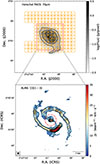 |
Fig. 1. Upper panel: JCMT observing positions of NGC 1068 overlaid on a Herschel/PACS 70 μm grayscale map. The black contours indicate the 70 μm continuum, starting from 100σ and increasing in steps of 3σ, where 1σ = 3 × 10⁻⁴ Jy/pixel. The white cross denotes the position of the central AGN in the galaxy. Orange circles indicate the positions observed in jiggle mapping mode. The red square shows the area (1.5′ × 1.5′) studied in this work. Bottom panel: Zoomed-in view of the central region obtained from the ALMA high-resolution CO (1–0) map (project ID: 2018.1.01684.S, Saito et al. 2022b; see also Nakajima et al. 2023). Black contours represent CO (1–0) integrated intensity levels, ranging from 4σ to 20σ in steps of 4σ, where 1σ = 0.25 Jy beam−1 km s−1. The dotted-dashed red circle represents the JCMT beam size of 14″ (approximately 1.1 kpc). |
2.2. Data reduction
Data reduction for the HCN (4 − 3) and HCO+ (4 − 3) observations was conducted using both the Continuum and Line Analysis Single-dish Software (CLASS)1, which is part of the GILDAS package developed by the Institut de radioastronomie millimétrique (IRAM), and STARLINK, a package developed for JCMT data reduction.
We first identified and flagged bad sub-scans through visual inspection using GAIA, a visualization tool within the STARLINK software suite. Flagged sub-scans were excluded by applying masks via the chpix task. In addition, high-noise regions located at the spectral edges of each sub-scan were removed to improve data quality. Following this, the data were converted from the STARLINK N-dimensional data format (NDF) format to the GILDAS/CLASS format. Reduction procedures were then applied individually to each sub-scan using the CLASS software. Spikes at the edges of the spectra and corrupted channels were replaced with Gaussian noise to minimize artifacts. Baseline subtraction was performed using either first- or second-order polynomial fitting, depending on the quality of the spectra. For positions with a signal-to-noise ratio (S/N) less than 3, the CO spectra were used to define appropriate baseline windows. All spectra were smoothed to a velocity resolution of 26 km s−1. The processed data were then converted back to the NDF format for further reduction using the ORAC-DR pipeline, an automated data reduction procedure developed specifically for JCMT observations within the STARLINK software suite (Jenness et al. 2015).
2.3. Ancillary data
To investigate the extended gas properties, we used ancillary CO(3–2) and CO (1–0) data. Archival IR and X-ray observations were used to derive the IR and X-ray luminosities.
2.3.1. CO (3-2) and CO (1-0) data
The CO (3 − 2) data were retrieved from the JCMT archive (project ID: M09BC05) and were observed using HARP and ACSIS, with a FWHM beam size of approximately 14″, comparable to the MALATANG data. This observation used scan mode, also known as raster mode, which is the most efficient observing mode for large maps. During the scans, the HARP array was rotated at a specific angle, resulting in a sampling spacing of 10.3″.
The CO (1 − 0) data were obtained from the Nobeyama CO Atlas of Nearby Spiral Galaxies2, using the Nobeyama Radio Observatory (NRO) 45 m Telescope (Kuno et al. 2007). The beam size FWHM is about 15″, which is comparable to our MALATANG data.
The reduction of the CO (1 − 0) data was performed using the CLASS software, while the CO (3 − 2) were reduced following the standard JCMT data reduction procedures. The CO (1 − 0) and CO (3 − 2) maps were re-gridded to a common pixel size of 10″, consistent with the MALATANG data.
2.3.2. Infrared data
To investigate the IR characteristics of NGC 1068, we included the IR photometric data at 70 μm, 160 μm, and 850 μm bands. The 70 μm and 160 μm data were obtained from Herschel/PACS, with FWHM angular resolutions of approximately 5.8″ and 12″, respectively. To match the resolution of the MALATANG observations, the Herschel maps were convolved using the convolution kernels provided by Aniano et al. (2011) to achieve a common beam size of 14″. The maps were then scaled by a factor of 1.133 × (14/pixel size)2 to convert the flux units from Jy to Jy beam−1, where the pixel size is in arcseconds.
The 850 μm data were obtained from the Submillimetre Common-User Bolometer Array 2 (SCUBA2) on the JCMT, with a FWHM of approximately 14.6″. To convert the flux units from pW to Jy, we used the standard Flux Conversion Factor of 2.13 ± 0.12 Jy pW−1 arcsec−2 for the 850 μm data.
2.3.3. X-ray data
We used the Chandra observation conducted in 2000 (ObsID 344) with an exposure time of 47.44 ks and a beam size of approximately 0.5″. The data were reprocessed using CIAO v4.17 and CALDB v4.11.6. To obtain the emission of diffuse X-ray-emitting gas, we identified point sources by the wavelet-based source detection algorithm wavdetect (Freeman et al. 2002) in the energy range of 0.5–7 keV and on the wavelet scales of 1,  , 2, 2
 , 4, 4
 , and 8. The 90% energy-encircled ellipse was adopted for the source region based on the point spread function shape. To minimize ring-like artifacts from the point spread function wings, we manually increased the ellipse sizes for certain bright sources. The point source regions were then subtracted from the X-ray map. Given the Seyfert 2 AGN in the galaxy, we also removed the central region (approximately 8″ radius) of NGC 1068. The spectra of hot gas were extracted from regions corresponding to the size of the JCMT beam (14″) at each observation position, using the CIAO routine specextract, with the background region defined on the same CCD chip, excluding point sources and the target regions. We fitted the hot gas spectra using the XSPEC v.12.11.0 (Arnaud 1996) software with an absorbed Astrophysical Plasma Emission Code (APEC; Smith et al. 2001). The fitted X-ray luminosities were corrected for both Galactic and intrinsic absorption.
3. Result
3.1. Integrated intensity images
Figure 2 displays the spatial distributions of the integrated intensities for HCN (4 − 3), HCO+ (4 − 3), CO (3 − 2), and CO (1 − 0). All four tracers exhibit elongated morphologies along the southwest–northeast direction, aligning with the major axis of NGC 1068. The molecular gas traced by HCN (4 − 3) and HCO+ (4 − 3) is significantly more compact than the distributions seen in CO (1 − 0) and CO (3 − 2). We note that the distribution of HCO+ (4 − 3) is highly asymmetric compared to the other tracers, with more prominent emission in the western region than the eastern region. Both HCN (4 − 3) and HCO+ (4 − 3) emissions peak at the center, coinciding with the position of the AGN.
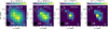 |
Fig. 2. Integrated intensity (moment 0) maps of molecular gas tracers, shown with a pixel size of 10″. (a): CO (1 − 0) map with contours at levels of 15–35σ in steps of 5σ (σ = 4.34 K km s−1). (b): CO (3 − 2) map with contours from 13 to 57σ in steps of 11σ (σ = 2.39 K km s−1). (c): HCN (4 − 3) map with contours from 3 to 12σ in steps of 3σ (σ = 0.38 K km s−1). (d): HCO+ (4 − 3) map with contours from 3 to 6σ in steps of 1σ (σ = 0.41 K km s−1). The white cross marks the location of the AGN in NGC 1068. Pixels with S/Ns below 3 are masked. The beam size and scale bar are shown in the lower-left corner of each panel. |
In contrast, CO (1 − 0) and CO (3 − 2) emissions exhibit their peak intensities in the southwestern region. Using interferometric data, Tsai et al. (2012) reported that CO (3 − 2) emission in NGC 1068 typically peaks at the nucleus, whereas CO (1 − 0) emission is predominantly distributed along the spiral arms. However, at our current resolution, the spatial distribution of CO (3 − 2) is similar to that of CO (1 − 0). In particular, the southwestern region shows the strongest CO (3 − 2) and CO (1 − 0) emissions, consistent with the SB knot within the pseudo-ring structure revealed in the ALMA CO (1 − 0) map (see Fig. 1). Spectral maps of these lines (Figure A1 and A2) are available on Zenodo.
3.2. Line and infrared luminosities
We calculated the line luminosities using the method described by Solomon et al. (1997):
 (1)
(1)
where S△v is the velocity-integrated flux density in units of Jy km s−1, and vobs is the observed line frequency in units of GHz. DL is the luminosity distance (see Table 1). To convert line intensity to flux density, we used the conversion factor S/Tmb = 15.6/ηmb, where ηmb is the main beam efficiency. We adopted ηmb(JCMT) = 0.64 and ηmb(NRO 45m) = 0.40.
The uncertainties of line intensity were derived from
 (2)
(2)
where Trms is the RMS main-beam temperature, △vres is the spectral velocity resolution, △vline is the velocity range of the emission line, and △vbase is the velocity range used to fit the baseline (Gao 1996; Matthews & Gao 2001). We adopted the velocity ranges of CO (3 − 2) as a reference for determining the spectral ranges used in the baseline fitting of the HCN (4 − 3) and HCO+ (4 − 3) lines at outer regions, since CO (3 − 2) emission is more spatially extended and exhibits similar kinematic properties as HCN (4 − 3) and HCO+ (4 − 3). Note that an additional 10% uncertainty is included to account for systematic errors in the absolute flux calibration.
To calculate the total IR luminosities (from 8 μm to 1000 μm) of NGC 1068, we estimated the resolved and integrated LTIR from Herschel bands with combined tracers (Galametz et al. 2013) as
 (3)
(3)
where νLν(i) is the resolved luminosity in units of L⊙, and ci is the calibration coefficients for the combination of different bands. For NGC 1068, the equation is LTIR = (1.010 ± 0.023) νLν (70 μm) + (1.218 ± 0.017) νLν(160 μm). The uncertainty in the LTIR calibration derived from the combination of multiple IR bands is adopted to be 25% (Galametz et al. 2013). Additionally, we assumed a 5% flux calibration uncertainty, following Balog et al. (2014).
The intensities, line luminosities of the four molecular tracers, and the total IR luminosities for individual resolved regions are listed in Appendix A. All uncertainties are estimated from the measurements using Eq. (2). For positions with S/Ns below 3, only 3σ upper limits are provided in the table.
3.3. Relation between dense gas tracers and IR luminosities
The term “dense gas” usually refers to molecular gas with nH2 > 104 cm−3 (Lada 1992). HCN (4–3) and HCO+ (4–3) have critical densities of approximately 2.3 × 107 cm−3 and 3.2 × 106 cm−3, respectively, at 20 K under optically thin assumptions (Shirley 2015). Given their high critical densities, we considered HCN (4–3) and HCO+ (4–3) to be tracers of dense molecular gas in this study.
We examine the correlations between the luminosities of molecular gas and the IR luminosities in Fig. 3. To improve the S/N in the outer regions, we averaged the spectra from pixels at the same radial distance to obtain stacked data. The HCN (4 − 3) and HCO+ (4 − 3) emissions are detected at approximately 3–8σ levels in the outer disk region (approximately 2.2–3.2 kpc radial distance) by stacking spectra from different radial positions (see Fig. A3, available on Zenodo). The LIR − L′dense correlation is consistent with the fitting results reported by Tan et al. (2018). Notably, despite the influence of AGN activity in the central regions of NGC 1068, all data points still follow the linear LIR − L′dense correlation. The impact of the AGN is discussed in Sect. 4.1.
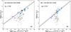 |
Fig. 3. Relations between IR luminosities and dense molecular line luminosities in logarithmic scale. (a): LIR − L′HCN(4 − 3). (b): LIR − L′HCO+(4 − 3). Detected data are shown as solid points, data points obtained from stacked spectra are shown as diamonds, and upper limits are marked by gray leftward arrows. The black circles highlight the central region of NGC 1068, which hosts the AGN. The Spearman rank correlation coefficients (ρsp) are displayed in each panel. The solid lines and their slopes (β) represent the best-fit results from Bayesian regression, as adopted from Tan et al. (2018). |
3.4. Relation between  and SFR
The diffuse soft X-ray emission (0.5–2 keV band) from hot gas produced by stellar feedback is found to correlate with the SFR, particularly in SB regions (e.g., Ranalli et al. 2003; Grimm et al. 2003; Zhang et al. 2024). We explored the relation between the diffuse thermal X-ray luminosity ( ) of the hot gas and the SFR (Fig. 4). Assuming that the IR luminosity is dominated by star formation, we estimated the SFR from the total IR luminosity using the relation given by Kennicutt (1998):
 (4)
(4)
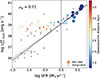 |
Fig. 4. Relation between SFR and thermal X-ray luminosity of hot gas on sub-kiloparsec scales. The color scale represents the distance from the galactic center, and the marker size represents the SFR surface density. The central data point containing the AGN has been excluded. The vertical dashed black line marks SFR = 1 M⊙ yr−1, corresponding to ΣSFR = 8.2 × 10⁻⁶ M⊙ yr−1 kpc−2. The solid black line represents the best-fit scaling relation as expressed in Eq. (5), derived from the central 12 data points with SFRs > 1 M⊙ yr−1. The Spearman rank correlation coefficient (ρsp) is provided. The gray crosses represent data from the central regions of nearby galaxies (Zhang et al. 2024), while the dashed gray line indicates the corresponding best-fit relation for these galaxies. |
where the LTIR is the total IR luminosity estimated by Eq. (3). Note that this relation is typically used to estimate the global SFR of entire galaxies. However, in this study, we applied it to spatially resolved regions under the assumption that the relation holds at sub-kiloparsec scales. The SFR surface density (ΣSFR) is calculated as the SFR within a region divided by its physical area:  , where A is the area over which the SFR is measured, in units of kpc2.
A bimodal pattern is found in this correlation, distinguishing the central region, where SFR > 1 M⊙ yr−1 (i.e., ΣSFR > 8.2 × 10⁻⁶ M⊙ yr−1 kpc−2) from the outer disk, where SFR < 1 M⊙ yr−1 (i.e., ΣSFR < 8.2 × 10⁻⁶ M⊙ yr−1 kpc−2), similar to the findings reported in M51 (Zhang et al. 2025). Variations between the central and disk regions indicate spatially distinct gas heating mechanisms within the galaxy. Central hot gas may primarily be heated by the combined influence of AGN activity and SB processes.
We used the Python package Linmix to perform Bayesian linear regression using Markov chain Monte Carlo sampling (Kelly 2007). We used only the central 12 data points (with radial distances < 1.7 kpc), where each region exhibits a high SFR surface density (ΣSFR > 8.2 × 10⁻⁶ M⊙ yr−1 kpc−2) and shows detections of both HCN(4–3) and HCO+(4–3). Using these data, the linear regression yields a super linear relation with a Spearman rank correlation coefficient of 0.71 and a p-value of 0.01 (solid black line in Fig. 4):
 (5)
(5)
The X-ray luminosity ranges from 1038 to 1041 erg s−1, which is broadly consistent with the soft-band luminosities typically found in nearby star-forming galaxies at the sub-kiloparsec scale (e.g., Zhang et al. 2024). The  – SFR relation shows a significant excess over the linear trend, consistent with the findings of Zhang et al. (2024), as indicated in Fig. 4. This super-linear relation is likely driven by the extreme conditions in galaxy centers, including AGN activity and intense star formation, both of which contribute to the accumulation of hot gas at the galactic center. Furthermore, AGNs may influence X-ray and IR emissions with different efficiencies, which could further contribute to the super-linear correlation.
4. Analysis and discussion
4.1. AGN feedback effects
Both star formation and AGN activity can heat the surrounding dust and gas, leading to enhanced IR luminosity and elevated molecular line emission (e.g., Krips et al. 2008; Izumi et al. 2013). In particular, the CND in NGC 1068 is strongly influenced by ionized winds driven by the AGN (e.g., García-Burillo et al. 2014), which contribute to high temperatures that further enhance the abundances of molecules (e.g., Harada et al. 2010). The spatial resolution of our JCMT observations is insufficient to disentangle the AGN, CND, and SB ring. Therefore, both the central beam (covering the AGN and the CND) and nearby beam-covered regions in our observations are likely influenced by the combined effects of the CND and the AGN. As mentioned in Sect. 3.1, the emissions of HCN (4-3) and HCO+ (4-3) are likely enhanced by AGN-driven radiation in the central region of NGC 1068. However, AGN activity does not appear to significantly affect the LIR − L′dense relation, which remains consistent with the general trend of the star formation law, as presented in Sect. 3.3.
A plausible explanation is that the influence of AGN activity in NGC 1068 is localized rather than galaxy-wide. Esquej et al. (2014) indicates that AGN radiation has no significant impact on star formation at scales of approximately 100 pc from the nucleus. Similarly, a research toward nearby AGN-hosting galaxies by Esposito et al. (2022) found no significant evidence of AGN influence on the molecular gas properties at kiloparsec scales. Although the mechanical feedback from AGNs, such as jets and outflows, can extend over several kiloparsecs (García-Burillo et al. 2014; Saito et al. 2022a), star formation is the dominant contributor to the total IR luminosity in AGN-embedded systems (Nardini et al. 2008; Vivian et al. 2012). A study of NGC 1068 by Tsai et al. (2012) indicates that while the molecular gas in the nuclear region is influenced by AGN radiation, the gas in the spiral arms is mainly affected by star formation. As suggested by Juneau et al. (2009), HCN can serve as a reliable tracer of the dense gas responsible for star formation, even in the presence of AGNs. Moreover, the extremely short timescale of the AGN outflow (approximately 0.2 Myr; Das et al. 2006) suggests that AGN feedback has only a minor influence at the current stage. Alternatively, AGNs could affect the IR and molecular line emissions in a comparable way, which could explain why the central region still follows the linear LIR − L′dense relation.
The AGN is estimated to contribute approximately 10% of the diffuse X-ray luminosity within the central region of M51 (Terashima & Wilson 2001). Smith et al. (2018) demonstrates that the  /SFR ratio remains unaffected by AGN activity, supporting the interpretation that diffuse soft X-ray emission is primarily powered by feedback from stars and supernovae. Therefore, the AGN contribution to the soft-band X-ray luminosity is also relatively small in the outer region. Note that the observed diffuse X-ray emission may also include contributions from faint, unresolved point sources such as X-ray binaries, cataclysmic variables, active binaries, supernova remnants, and young stellar objects. However, these compact sources contribute only minimally to the total soft X-ray emission (Kuntz & Snowden 2010; Wang et al. 2021; Zhang & Wang 2025).
4.2. Dust temperature dependence of molecular line ratios
To derive the dust temperatures and column densities in NGC 1068, we performed spectral energy distribution (SED) fitting using IR data at 70 μm, 160 μm, and 850 μm. We described the dust radiation by a single modified blackbody model, and thus the observed flux density (Sν) is related to the Planck function Bν(T) as
 (6)
(6)
where τν is the optical depth at frequency ν, and Ω is the solid angle of the source in steradians.
The total column density NH2 is then
 (7)
(7)
where μ is the mean molecular mass per hydrogen atom, mH is the hydrogen mass, and a gas-to-dust ratio of 100 is assumed. The dust emissivity κν at a given frequency is calculated as
 (8)
(8)
where β is the emissivity index, and κ230 is the dust opacity at 230 GHz. In this work, we adopted κ230 = 0.899 cm2g−1, following Ossenkopf & Henning (1994).
To ensure consistency in spatial resolution, all IR maps were convolved to match the beam size (14″) of the MALATANG data. The SED fitting was then performed on a grid of 9 × 9 pixels to derive spatially resolved maps of dust temperature and column density. The total flux uncertainty accounts for contributions from photometric measurement errors, a 5% flux calibration uncertainty, and an additional 5% systematic uncertainty, following Balog et al. (2014). Note that background and foreground emissions were not subtracted from the IR images.
In the SED fitting, the emissivity index β was set as a free parameter. We obtained an average value of β = 1.94 for NGC 1068, which is broadly consistent with the typical range in the galaxies of 1–2.5 (Chapin et al. 2011) and is close to the average value of approximately 1.78 found in the Galactic disk (Planck Collaboration XXV 2011). The SED fitting results at representative positions are presented in Appendix B. In the central region, the SED fitting reveals a dust temperature of 32.8 ± 0.6 K and a column density NH2 of 1.6 × 1022 cm−2, which is consistent with the cold dust SED results of NGC 1068 in Zhou et al. (2022).
We explored the relationships between the molecular line ratios and the dust temperature of NGC 1068, as shown in Fig. 5. The integrated intensity ratios HCN (4–3)/CO (1–0) and HCO+ (4–3)/CO (1–0) serve as proxies for dense and warm gas fraction, since HCN (4–3) and HCO+ (4–3) have higher critical densities and excitation requirements compared to CO (1–0). Meanwhile, R31, defined as ICO(3 − 2)/ICO(1 − 0), is a key diagnostic of molecular gas excitation conditions (Mauersberger et al. 1999; Wang et al. 2025).
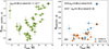 |
Fig. 5. (a): Correlation between dust temperature and gas excitation (traced by R31). (b): Correlation between dust temperature and dense and warm gas fraction, denoted by HCN (4 − 3)/CO (1 − 0) and HCO+ (4 − 3)/CO (1 − 0) integrated intensity ratios. Black circles denote the central position of NGC 1068, which hosts the AGN. The Spearman rank correlation coefficients are shown at each panel. |
Our result reveals a positive correlation between Tdust and R31, with a Spearman rank coefficient of ρsp = 0.60 and a p-value of 9.7 × 10⁻⁶. The mean R31 value of 0.5 ± 0.1 is consistent with previously reported values for this galaxy (Mauersberger et al. 1999; Mao et al. 2010). Although the central region of NGC 1068 is likely dominated by X-ray-dominated regions (XDRs; Hailey-Dunsheath et al. 2012), where intense X-ray radiation from the AGN can heat the gas via photoionization and potentially cause dust–gas decoupling, our results show that this region still follows the positive correlation. This correlation indicates that dust temperature is linked to molecular gas excitation, suggesting that the dust and molecular gas are likely thermally coupled (e.g., Young et al. 1986; Goldsmith 2001).
A similar positive correlation is found between the HCN (4 − 3)/CO(1 − 0) integrated intensity ratio and Tdust, with a Spearman rank coefficient of ρsp = 0.68 and a p-value of 0.01. The positive correlation between HCN (4–3)/CO (1–0) and Tdust, particularly in the central region of the galaxy, can be attributed to AGN feedback, which enhances star formation activity and simultaneously heats both the dust and the dense molecular gas traced by HCN (4–3). However, there is no clear correlation found between HCO+(4-3)/CO(1-0) intensity ratio and Tdust. HCO+ (4-3) traces denser, more shielded gas components compared to CO (3-2), whose excitation conditions are less affected by variations in dust temperature (e.g., Papadopoulos et al. 2014). Moreover, the fractional abundance of HCO+ is less sensitive to AGN-driven chemistry than that of HCN. These factors could lead to the weak or absent correlation between HCO+(4–3)/CO(1–0) and Tdust, whereas stronger correlations are found for both R31–Tdust and HCN(4–3)/CO(1–0)–Tdust.
4.3. Relation between  /SFR and dense gas
As presented in Sect. 3.4, we find a super-linear relationship between  and the SFR. The X-ray-to-SFR ratio (
 ) indicates the relative contribution of hot gas emission compared to star formation. To explore the possible correlation between this relative contribution and dense gas, we further investigated the relationships between
  and the integrated intensity ratios CO(3–2)/CO(1–0), HCN(4–3)/CO(1–0), and HCO+(4–3)/CO(1–0) (Fig. 6). As the outer regions of the galaxy lack detectable dense gas, our analysis focuses solely on the central region, where HCN (4-3) or HCO+ (4-3) is detected with S/N > 3, while excluding the central point that may be strongly influenced by the AGN. The ratio of soft X-ray luminosity to SFR (
 /SFR) represents the soft X-ray emission per unit SFR and serves as a valuable tracer of stellar feedback in star-forming galaxies. We obtain log
  /SFR = 38.5–40.3 erg s−1 (M⊙ yr−1)−1 for NGC 1068, which is consistent with the values from merging galaxies reported by Smith et al. (2018).
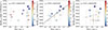 |
Fig. 6. Relations between line ratios and |

We find no significant correlation between the X-ray-to-SFR ratio and R31, nor between the X-ray-to-SFR luminosity ratio and RHCO+(4 − 3)/CO(1 − 0). In contrast, a linear relationship is found between the X-ray-to-IR luminosity ratio and RHCN(4 − 3)/CO(1 − 0) as follows:
 (9)
(9)
The correlation yields a Spearman rank coefficient of ρsp = 0.75 and a p-value of 0.02. This positive correlation may arise from the relative contributions of different evolutionary stages of the star formation process, since  traces hot gas heated after star formation, SFR traced by the total IR luminosity reflects recent or ongoing star formation (Kennicutt & Evans 2012), HCN (4–3) traces the dense gas directly involved in star formation, and CO (1–0) traces the cold gas reservoir.
While both HCN and HCO+ trace dense molecular gas, HCN (4–3) has a critical density about one order of magnitude higher than that of HCO+(4–3), as mentioned in Sect. 3.3. Given that their critical densities are relatively similar, it is unlikely that the difference in the correlation arises from the critical density itself. The emission of HCN is strongly affected by IR radiative pumping (e.g., Matsushita et al. 2015; Stuber et al. 2023) and XDR chemistry (e.g., Lepp & Dalgarno 1996; Meijerink et al. 2007), whereas HCO+ and CO are comparatively less impacted by these processes. Consequently, the HCN/CO ratio may more effectively trace the high-energy feedback, which may account for the observed super-linear correlation with  /SFR.
/SFR.
Models and observations show that both XDR chemistry and IR radiative pumping are confined to the nuclear region near the AGN in the galaxy (e.g., Esposito et al. 2022). Beyond this scale, their influence on molecular excitation rapidly diminishes. Moreover, Pérez-Beaupuits et al. (2007) proposed that photon-dominated regions account for the dominant excitation mechanism in the molecular gas in NGC 1068. Note that the found super-linear correlation between  /SFR and HCN/CO extends beyond the central region, reaching distances greater than 2 kpc. Therefore, molecular excitation is most likely governed by AGN-related mechanisms in the nuclear region, while star formation becomes the dominant contributor in the outer regions, particularly beyond 2 kpc.
The relative enhancement of HCN emission with respect to HCO+ can serve as a diagnostic of energetic processes such as AGN activity (Imanishi & Nakanishi 2014). We found that the RHCN/HCO+(4 − 3) values range from 1 to 3, with a ratio of approximately 2 at the galaxy center. This central enhancement is significantly higher than that observed in normal or SB galaxies, for which Tan et al. (2018) reported an average RHCN/HCO+(4 − 3) of 0.8 ± 0.5 in systems without embedded AGNs. However, it is unexpected that the highest RHCN/HCO+43 value in NGC 1068 is found off-center, reaching ∼3 at an offset of (0, −10). Bešlić et al. (2021) reported that the highest HCN/HCO+ ratio in NGC 3627 occurs in the bar region (approximately 2 kpc), suggesting that environments such as bars and SB rings can enhance HCN abundance. The elevated RHCN/HCO+(4 − 3) observed at ∼1.5 kpc in NGC 1068 may therefore indicate that the SB ring contributes to the enhancement of HCN emission, similar to the findings of Privon et al. (2015).
Therefore, the HCN (4-3)/CO (1-0) ratio in relation to  /SFR may originate from the excitation mechanisms associated with both AGN activity and star formation. However, the correlations are based on a small number of data points and should therefore be interpreted with caution. To verify the correlation observed in NGC 1068 and explore its underlying mechanisms, observations with higher sensitivity and spatial resolution, together with studies extended to a larger sample, will be required.
5. Summary
In this paper we present the HCN (4 − 3) and HCO+ (4 − 3) observational results of NGC 1068 from the MALATANG project, covering a region of approximately 1.5′ × 1.5′. Based on sub-scan-level data reduction and incorporating spectral stacking techniques, we improved the S/N in the outer disk regions. Our main conclusions are as follows:
-
(1)
Using spectral stacking, we detected HCN (4–3) and HCO+ (4–3) emissions at approximately 3–8σ levels in the outer disk (∼2.2–3.2 kpc radial distance) of NGC 1068.
-
(2)
The spatially resolved LIR − L′dense relations of NGC 1068, determined using HCN (4-3) and HCO+ (4-3) as dense gas tracers, are found to be linear. Although the central data points could be significantly influenced by AGN activity, they do not deviate noticeably from the overall correlation.
-
(3)
Using SED fitting, we derived a dust temperature map and found a strong positive correlation between Tdust and R31 with a Spearman rank coefficient of ρsp = 0.60, indicating that dust and molecular gas are thermally coupled. A similar positive correlation between HCN (4–3)/CO (1–0) and Tdust (ρsp = 0.68), particularly in the central region of the galaxy, may be due to AGN feedback. However, HCO+/CO shows no correlation with Tdust.
-
(4)
A twofold correlation is found between the spatially resolved soft X-ray emission (
 ) and the SFR across the galaxy, implying the presence of different feedback mechanisms linked to star formation activity. In the central region, this results in a statistically significant super-linear relationship with a slope of 2.2.
 -
(5)
A super-linear relationship is found between the soft X-ray to SFR ratio (
 /SFR) and the HCN(4–3)/CO(1–0) ratio, with a fitted slope of 1.34, which may arise from the differing contributions of various evolutionary stages in the star formation process. In contrast, this trend is not apparent for the HCO+(4–3)/CO(1–0) or CO(3–2)/CO(1–0) ratios.
Data availability
Figures A1–A3 are only available in electronic form at Zenodo via url (https://doi.org/10.5281/zenodo.17741281). Table A1 is available at the CDS via https://cdsarc.cds.unistra.fr/viz-bin/cat/J/A+A/707/A20.
Acknowledgments
S.L. and S.F. acknowledge support from the National Key R&D program of China grant (2025YFE0108200), National Science Foundation of China (12373023, 12133008), the starting grant at Xiamen University, and the presidential excellence fund at Xiamen University. This work is supported by the China Manned Space Program with grant no.CMS-CSST-2025-A10. Z.Y.Z acknowledges the support of NSFC (grants 12041305, 12173016), and the Program for Innovative Talents, Entrepreneur in Jiangsu. Q.T. acknowledges support from the NSFC (grants 12033004, 12573013). Y.G. acknowledges the project ZR2024QA212 supported by Shandong Provincial Natural Science Foundation, National Natural Science Foundation of China (NSFC, Nos.12033004 and 12233005), and Scientific Research Fund of Dezhou University (3012304024). X.-L.W. acknowledges the support by the Science Foundation of Hebei Normal University (grant No. L2024B56) and S&T Program of Hebei (grant No. 22567617H). K.K. acknowledges the support by JSPS KAKENHI Grant Numbers JP17H06130, JP20H00172, JP23K20035 and JP24H00004. T.T. acknowledges the support by the NAOJ ALMA Scientific Research Grant Number 2020-15A. J.W. acknowledges the support of NSFC grants 12033004 and 12333002. The James Clerk Maxwell Telescope is operated by the East Asian Observatory on behalf of The National Astronomical Observatory of Japan, Academia Sinica Institute of Astronomy and Astrophysics, the Korea Astronomy and Space Science Institute, the National Astronomical Observatories of China and the Chinese Academy of Sciences, with additional funding support from the Science and Technology Facilities Council of the United Kingdom and participating universities in the United Kingdom and Canada. MALATANG is a JCMT Large Program with project codes of M16AL007 and M20AL022. We acknowledge the ORAC-DR, STARLINK, and GILDAS software for the data reduction and analysis. This research has made use of Chandra archival data and software provided by the Chandra X-ray Center (CXC) in the application package CIAO. This research has also made use of the NASA/IPAC Extragalactic Database (NED), which is operated by the Jet Propulsion Laboratory, California Institute of Technology, under contract with the National Aeronautics and Space Administration. The Chandra data archive is maintained by the Chandra X-ray Center at the Smithsonian Astrophysical Observatory. This paper is dedicated to the memory of the late Professor Yu Gao, co-PI of the MALATANG project.
References
- Aniano, G., Draine, B. T., Gordon, K. D., & Sandstrom, K. 2011, PASP, 123, 1218 [Google Scholar]
- Arnaud, K. A. 1996, in Astronomical Data Analysis Software and Systems V, eds. G. H. Jacoby, & J. Barnes, ASP Conf. Ser., 101, 17 [NASA ADS] [Google Scholar]
- Balog, Z., Müller, T., Nielbock, M., et al. 2014, Exp. Astron., 37, 129 [Google Scholar]
- Bešlić, I., Barnes, A. T., Bigiel, F., et al. 2021, MNRAS, 506, 963 [CrossRef] [Google Scholar]
- Bigiel, F., Leroy, A., Walter, F., et al. 2008, AJ, 136, 2846 [NASA ADS] [CrossRef] [Google Scholar]
- Capetti, A., Macchetto, F. D., & Lattanzi, M. G. 1997, ApJ, 476, L67 [NASA ADS] [CrossRef] [Google Scholar]
- Chapin, E. L., Chapman, S. C., Coppin, K. E., et al. 2011, MNRAS, 411, 505 [Google Scholar]
- Choi, E., Ostriker, J. P., Naab, T., Oser, L., & Moster, B. P. 2015, MNRAS, 449, 4105 [CrossRef] [Google Scholar]
- Cox, T. J., Dutta, S. N., Di Matteo, T., et al. 2006, ApJ, 650, 791 [Google Scholar]
- Das, V., Crenshaw, D. M., Kraemer, S. B., & Deo, R. P. 2006, AJ, 132, 620 [Google Scholar]
- Esposito, F., Vallini, L., Pozzi, F., et al. 2022, MNRAS, 512, 686 [NASA ADS] [CrossRef] [Google Scholar]
- Esquej, P., Alonso-Herrero, A., González-Martín, O., et al. 2014, ApJ, 780, 86 [Google Scholar]
- Evans, N. J., II., Heiderman, A., & Vutisalchavakul, N. 2014, ApJ, 782, 114 [CrossRef] [Google Scholar]
- Federrath, C., & Klessen, R. S. 2012, ApJ, 761, 156 [Google Scholar]
- Freeman, P. E., Kashyap, V., Rosner, R., & Lamb, D. Q. 2002, ApJS, 138, 185 [Google Scholar]
- Galametz, M., Kennicutt, R. C., Calzetti, D., et al. 2013, MNRAS, 431, 1956 [NASA ADS] [CrossRef] [Google Scholar]
- Gámez Rosas, V., van der Werf, P., Gallimore, J. F., et al. 2025, A&A, 699, A187 [NASA ADS] [CrossRef] [EDP Sciences] [Google Scholar]
- Gao, Y. 1996, Ph.D. Thesis, State University of New York at Stony Brook [Google Scholar]
- Gao, Y., & Solomon, P. M. 2004a, ApJS, 152, 63 [Google Scholar]
- Gao, Y., & Solomon, P. M. 2004b, ApJ, 606, 271 [NASA ADS] [CrossRef] [Google Scholar]
- Gao, Y., Carilli, C. L., Solomon, P. M., & Vanden Bout, P. A. 2007, ApJ, 660, L93 [NASA ADS] [CrossRef] [Google Scholar]
- García-Burillo, S., Combes, F., Usero, A., et al. 2014, A&A, 567, A125 [Google Scholar]
- Gilfanov, M., Grimm, H.-J., & Sunyaev, R. 2004, MNRAS, 347, L57 [NASA ADS] [CrossRef] [Google Scholar]
- Goldsmith, P. F. 2001, ApJ, 557, 736 [Google Scholar]
- Grimm, H.-J., Gilfanov, M., & Sunyaev, R. 2003, MNRAS, 339, 793 [NASA ADS] [CrossRef] [Google Scholar]
- Hailey-Dunsheath, S., Sturm, E., Fischer, J., et al. 2012, ApJ, 755, 57 [NASA ADS] [CrossRef] [Google Scholar]
- Harada, N., Herbst, E., & Wakelam, V. 2010, ApJ, 721, 1570 [NASA ADS] [CrossRef] [Google Scholar]
- Heiderman, A., Evans, N. J., II., Allen, L. E., Huard, T., & Heyer, M. 2010, ApJ, 723, 1019 [NASA ADS] [CrossRef] [Google Scholar]
- Howell, J. H., Armus, L., Mazzarella, J. M., et al. 2010, ApJ, 715, 572 [Google Scholar]
- Imanishi, M., & Nakanishi, K. 2014, AJ, 148, 9 [NASA ADS] [CrossRef] [Google Scholar]
- Izumi, T., Kohno, K., Martín, S., et al. 2013, PASJ, 65, 100 [NASA ADS] [Google Scholar]
- Jenness, T., Currie, M. J., Tilanus, R. P. J., et al. 2015, MNRAS, 453, 73 [Google Scholar]
- Juneau, S., Narayanan, D. T., Moustakas, J., et al. 2009, ApJ, 707, 1217 [NASA ADS] [CrossRef] [Google Scholar]
- Kelly, B. C. 2007, ApJ, 665, 1489 [Google Scholar]
- Kennicutt, R. C., Jr. 1998, ApJ, 498, 541 [Google Scholar]
- Kennicutt, R. C., & Evans, N. J. 2012, ARA&A, 50, 531 [NASA ADS] [CrossRef] [Google Scholar]
- Krips, M., Neri, R., García-Burillo, S., et al. 2008, ApJ, 677, 262 [NASA ADS] [CrossRef] [Google Scholar]
- Krips, M., Martín, S., Eckart, A., et al. 2011, ApJ, 736, 37 [NASA ADS] [CrossRef] [Google Scholar]
- Krumholz, M. R., & McKee, C. F. 2005, ApJ, 630, 250 [Google Scholar]
- Krumholz, M. R., & Thompson, T. A. 2007, ApJ, 669, 289 [NASA ADS] [CrossRef] [Google Scholar]
- Kuno, N., Sato, N., Nakanishi, H., et al. 2007, PASJ, 59, 117 [NASA ADS] [Google Scholar]
- Kuntz, K. D., & Snowden, S. L. 2010, ApJS, 188, 46 [NASA ADS] [CrossRef] [Google Scholar]
- Lada, E. A. 1992, ApJ, 393, L25 [NASA ADS] [CrossRef] [Google Scholar]
- Lada, C. J., Lombardi, M., & Alves, J. F. 2010, ApJ, 724, 687 [Google Scholar]
- Lada, C. J., Forbrich, J., Lombardi, M., & Alves, J. F. 2012, ApJ, 745, 190 [NASA ADS] [CrossRef] [Google Scholar]
- Lee, J., Whitmore, B., Thilker, D., et al. 2021, American Astronomical Society Meeting Abstracts, 238, 331.04 [Google Scholar]
- Lepp, S., & Dalgarno, A. 1996, A&A, 306, L21 [NASA ADS] [Google Scholar]
- Leroy, A. K., Schinnerer, E., Hughes, A., et al. 2021, ApJS, 257, 43 [NASA ADS] [CrossRef] [Google Scholar]
- Liu, L., Gao, Y., & Greve, T. R. 2015, ApJ, 805, 31 [Google Scholar]
- Mao, R.-Q., Schulz, A., Henkel, C., et al. 2010, ApJ, 724, 1336 [Google Scholar]
- Matsushita, S., Trung, D.-V., Boone, F., et al. 2015, ApJ, 799, 26 [NASA ADS] [CrossRef] [Google Scholar]
- Matthews, L. D., & Gao, Y. 2001, ApJ, 549, L191 [Google Scholar]
- Mauersberger, R., Henkel, C., Walsh, W., & Schulz, A. 1999, A&A, 341, 256 [NASA ADS] [Google Scholar]
- Meijerink, R., Spaans, M., & Israel, F. P. 2007, A&A, 461, 793 [NASA ADS] [CrossRef] [EDP Sciences] [Google Scholar]
- Mountrichas, G., Masoura, V. A., Corral, A., & Carrera, F. J. 2024, A&A, 683, A143 [NASA ADS] [CrossRef] [EDP Sciences] [Google Scholar]
- Nagashima, Y., Saito, T., Ikarashi, S., et al. 2024, ApJ, 974, 243 [Google Scholar]
- Nakajima, T., Takano, S., Tosaki, T., et al. 2023, ApJ, 955, 27 [NASA ADS] [CrossRef] [Google Scholar]
- Nardini, E., Risaliti, G., Salvati, M., et al. 2008, MNRAS, 385, L130 [NASA ADS] [Google Scholar]
- Nguyen-Luong, Q., Nguyen, H. V. V., Motte, F., et al. 2016, ApJ, 833, 23 [NASA ADS] [CrossRef] [Google Scholar]
- Onodera, S., Kuno, N., Tosaki, T., et al. 2010, ApJ, 722, L127 [NASA ADS] [CrossRef] [Google Scholar]
- Ossenkopf, V., & Henning, T. 1994, A&A, 291, 943 [NASA ADS] [Google Scholar]
- Osterbrock, D. E., & Martel, A. 1993, ApJ, 414, 552 [Google Scholar]
- Papadopoulos, P. P., Zhang, Z.-Y., Xilouris, E. M., et al. 2014, ApJ, 788, 153 [CrossRef] [Google Scholar]
- Pérez-Beaupuits, J. P., Aalto, S., & Gerebro, H. 2007, A&A, 476, 177 [NASA ADS] [CrossRef] [EDP Sciences] [Google Scholar]
- Planck Collaboration XXV. 2011, A&A, 536, A25 [NASA ADS] [CrossRef] [EDP Sciences] [Google Scholar]
- Privon, G. C., Herrero-Illana, R., Evans, A. S., et al. 2015, ApJ, 814, 39 [CrossRef] [Google Scholar]
- Ranalli, P., Comastri, A., & Setti, G. 2003, A&A, 399, 39 [NASA ADS] [CrossRef] [EDP Sciences] [Google Scholar]
- Saito, T., Takano, S., Harada, N., et al. 2022a, ApJ, 927, L32 [NASA ADS] [CrossRef] [Google Scholar]
- Saito, T., Takano, S., Harada, N., et al. 2022b, ApJ, 935, 155 [NASA ADS] [CrossRef] [Google Scholar]
- Sánchez-García, M., García-Burillo, S., Pereira-Santaella, M., et al. 2022, A&A, 660, A83 [NASA ADS] [CrossRef] [EDP Sciences] [Google Scholar]
- Santini, P., Rosario, D. J., Shao, L., et al. 2012, A&A, 540, A109 [NASA ADS] [CrossRef] [EDP Sciences] [Google Scholar]
- Schinnerer, E., Eckart, A., Tacconi, L. J., Genzel, R., & Downes, D. 2000, ApJ, 533, 850 [Google Scholar]
- Schinnerer, E., Meidt, S. E., Pety, J., et al. 2013, ApJ, 779, 42 [Google Scholar]
- Shimizu, T. T., Mushotzky, R. F., Meléndez, M., Koss, M., & Rosario, D. J. 2015, MNRAS, 452, 1841 [NASA ADS] [CrossRef] [Google Scholar]
- Shirley, Y. L. 2015, PASP, 127, 299 [Google Scholar]
- Simkin, S. M., Su, H. J., & Schwarz, M. P. 1980, ApJ, 237, 404 [NASA ADS] [CrossRef] [Google Scholar]
- Smith, R. K., Brickhouse, N. S., Liedahl, D. A., & Raymond, J. C. 2001, ApJ, 556, L91 [Google Scholar]
- Smith, B. J., Campbell, K., Struck, C., et al. 2018, AJ, 155, 81 [NASA ADS] [CrossRef] [Google Scholar]
- Solomon, P. M., Downes, D., Radford, S. J. E., & Barrett, J. W. 1997, ApJ, 478, 144 [NASA ADS] [CrossRef] [Google Scholar]
- Springel, V., & Hernquist, L. 2005, ApJ, 622, L9 [Google Scholar]
- Stuber, S. K., Pety, J., Schinnerer, E., et al. 2023, A&A, 680, L20 [NASA ADS] [CrossRef] [EDP Sciences] [Google Scholar]
- Tan, Q.-H., Gao, Y., Zhang, Z.-Y., et al. 2018, ApJ, 860, 165 [NASA ADS] [CrossRef] [Google Scholar]
- Terashima, Y., & Wilson, A. S. 2001, ApJ, 560, 139 [Google Scholar]
- Tosaki, T., Kohno, K., Harada, N., et al. 2017, PASJ, 69, 18 [NASA ADS] [Google Scholar]
- Tsai, M., Hwang, C.-Y., Matsushita, S., Baker, A. J., & Espada, D. 2012, ApJ, 746, 129 [NASA ADS] [CrossRef] [Google Scholar]
- Usero, A., Leroy, A. K., Walter, F., et al. 2015, AJ, 150, 115 [Google Scholar]
- Vivian, U., Sanders, D. B., Mazzarella, J. M., et al. 2012, ApJS, 203, 9 [CrossRef] [Google Scholar]
- Wang, J., Zhang, Z.-Y., Qiu, J., et al. 2014, ApJ, 796, 57 [CrossRef] [Google Scholar]
- Wang, Q. D., Zeng, Y., Bogdán, Á., & Ji, L. 2021, MNRAS, 508, 6155 [NASA ADS] [CrossRef] [Google Scholar]
- Wang, J.-F., Gao, Y., Tan, Q.-H., et al. 2025, A&A, 700, A72 [NASA ADS] [CrossRef] [EDP Sciences] [Google Scholar]
- Wu, J., Evans, N. J., I., Gao, Y., et al. 2005, ApJ, 635, L173 [NASA ADS] [CrossRef] [Google Scholar]
- Xu, C. K., Cao, C., Lu, N., et al. 2015, ApJ, 799, 11 [Google Scholar]
- Young, J. S., Schloerb, F. P., Kenney, J. D., & Lord, S. D. 1986, ApJ, 304, 443 [NASA ADS] [CrossRef] [Google Scholar]
- Zhang, C., & Wang, J. 2025, ApJ, 988, 263 [Google Scholar]
- Zhang, Z.-Y., Gao, Y., Henkel, C., et al. 2014, ApJ, 784, L31 [NASA ADS] [CrossRef] [Google Scholar]
- Zhang, C., Wang, J., Tan, Q.-H., et al. 2024, ApJ, 967, L25 [Google Scholar]
- Zhang, C., Wang, J., & Cao, T.-W. 2025, ApJ, 978, L15 [Google Scholar]
- Zhou, J., Zhang, Z.-Y., Gao, Y., et al. 2022, ApJ, 936, 58 [NASA ADS] [CrossRef] [Google Scholar]
Appendix A: Table of intensities and luminosities
The intensities and luminosities of different tracers from individual resolved regions are available in electronic table at the CDS.
Appendix B: SED fitting results
Figure B.1 presents the dust SEDs of NGC 1068 at three representative positions: the galaxy center (0,0), a SB knot (-10, -10), and the outer disk (20, 30).
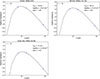 |
Fig. B.1. Dust SEDs of NGC 1068 at three representative positions: the galaxy center (0,0), a SB knot (-10,-10), and the outer disk (20,30). Blue dots represent the photometric data at 70 μm, 160 μm, and 850 μm, and the dashed lines represent the best-fit modified blackbody model. The fitting results are shown in the upper-left corner of each panel. |
All Tables
All Figures
|
Fig. 1. Upper panel: JCMT observing positions of NGC 1068 overlaid on a Herschel/PACS 70 μm grayscale map. The black contours indicate the 70 μm continuum, starting from 100σ and increasing in steps of 3σ, where 1σ = 3 × 10⁻⁴ Jy/pixel. The white cross denotes the position of the central AGN in the galaxy. Orange circles indicate the positions observed in jiggle mapping mode. The red square shows the area (1.5′ × 1.5′) studied in this work. Bottom panel: Zoomed-in view of the central region obtained from the ALMA high-resolution CO (1–0) map (project ID: 2018.1.01684.S, Saito et al. 2022b; see also Nakajima et al. 2023). Black contours represent CO (1–0) integrated intensity levels, ranging from 4σ to 20σ in steps of 4σ, where 1σ = 0.25 Jy beam−1 km s−1. The dotted-dashed red circle represents the JCMT beam size of 14″ (approximately 1.1 kpc). |
| In the text | |
|
Fig. 2. Integrated intensity (moment 0) maps of molecular gas tracers, shown with a pixel size of 10″. (a): CO (1 − 0) map with contours at levels of 15–35σ in steps of 5σ (σ = 4.34 K km s−1). (b): CO (3 − 2) map with contours from 13 to 57σ in steps of 11σ (σ = 2.39 K km s−1). (c): HCN (4 − 3) map with contours from 3 to 12σ in steps of 3σ (σ = 0.38 K km s−1). (d): HCO+ (4 − 3) map with contours from 3 to 6σ in steps of 1σ (σ = 0.41 K km s−1). The white cross marks the location of the AGN in NGC 1068. Pixels with S/Ns below 3 are masked. The beam size and scale bar are shown in the lower-left corner of each panel. |
| In the text | |
|
Fig. 3. Relations between IR luminosities and dense molecular line luminosities in logarithmic scale. (a): LIR − L′HCN(4 − 3). (b): LIR − L′HCO+(4 − 3). Detected data are shown as solid points, data points obtained from stacked spectra are shown as diamonds, and upper limits are marked by gray leftward arrows. The black circles highlight the central region of NGC 1068, which hosts the AGN. The Spearman rank correlation coefficients (ρsp) are displayed in each panel. The solid lines and their slopes (β) represent the best-fit results from Bayesian regression, as adopted from Tan et al. (2018). |
| In the text | |
|
Fig. 4. Relation between SFR and thermal X-ray luminosity of hot gas on sub-kiloparsec scales. The color scale represents the distance from the galactic center, and the marker size represents the SFR surface density. The central data point containing the AGN has been excluded. The vertical dashed black line marks SFR = 1 M⊙ yr−1, corresponding to ΣSFR = 8.2 × 10⁻⁶ M⊙ yr−1 kpc−2. The solid black line represents the best-fit scaling relation as expressed in Eq. (5), derived from the central 12 data points with SFRs > 1 M⊙ yr−1. The Spearman rank correlation coefficient (ρsp) is provided. The gray crosses represent data from the central regions of nearby galaxies (Zhang et al. 2024), while the dashed gray line indicates the corresponding best-fit relation for these galaxies. |
| In the text | |
|
Fig. 5. (a): Correlation between dust temperature and gas excitation (traced by R31). (b): Correlation between dust temperature and dense and warm gas fraction, denoted by HCN (4 − 3)/CO (1 − 0) and HCO+ (4 − 3)/CO (1 − 0) integrated intensity ratios. Black circles denote the central position of NGC 1068, which hosts the AGN. The Spearman rank correlation coefficients are shown at each panel. |
| In the text | |
|
Fig. 6. Relations between line ratios and |
| In the text | |
|
Fig. B.1. Dust SEDs of NGC 1068 at three representative positions: the galaxy center (0,0), a SB knot (-10,-10), and the outer disk (20,30). Blue dots represent the photometric data at 70 μm, 160 μm, and 850 μm, and the dashed lines represent the best-fit modified blackbody model. The fitting results are shown in the upper-left corner of each panel. |
| In the text | |
Current usage metrics show cumulative count of Article Views (full-text article views including HTML views, PDF and ePub downloads, according to the available data) and Abstracts Views on Vision4Press platform.
Data correspond to usage on the plateform after 2015. The current usage metrics is available 48-96 hours after online publication and is updated daily on week days.
Initial download of the metrics may take a while.