| Issue |
A&A
Volume 707, March 2026
|
|
|---|---|---|
| Article Number | A32 | |
| Number of page(s) | 17 | |
| Section | Cosmology (including clusters of galaxies) | |
| DOI | https://doi.org/10.1051/0004-6361/202557787 | |
| Published online | 25 February 2026 | |
CHEX-MATE: Relationship between X-ray and millimetre inferences of galaxy cluster temperature profiles
1
Dipartimento di Fisica, Università di Roma ‘Tor Vergata’ Via della Ricerca Scientifica 1 I-00133 Roma, Italy
2
INFN, Sezione di Roma ‘Tor Vergata’, Via della Ricerca Scientifica 1 00133 Roma, Italy
3
Space Science Data Center, Italian Space Agency Via del Politecnico 00133 Roma, Italy
4
High Energy Physics Division, Argonne National Laboratory Lemont IL 60439, USA
5
Dipartimento di Fisica, Sapienza Università di Roma Piazzale Aldo Moro 5 I-00185 Rome, Italy
6
Department of Astronomy, University of Geneva Ch. d’Ecogia 16 CH-1290 Versoix, Switzerland
7
INAF – Osservatorio di Astrofisica e Scienza dello Spazio di Bologna Via Piero Gobetti 93/3 I-40129 Bologna, Italy
8
INFN, Sezione di Bologna Viale Berti Pichat 6/2 I-40127 Bologna, Italy
9
Dipartimento di Fisica ‘E. Pancini’, Università degli Studi di Napoli Federico II, Via Cinthia 21 I-80126 Napoli, Italy
10
Center for Astrophysics | Harvard & Smithsonian 60 Garden Street Cambridge MA 02138, USA
11
Department of Physics, Informatics and Mathematics, University of Modena and Reggio Emilia 41125 Modena, Italy
12
INAF – IASF Milano Via A. Corti 12 I-20133 Milano, Italy
13
Dipartimento di Fisica e Astronomia (DIFA), Alma Mater Studiorum – Università di Bologna Via Gobetti 93/2 40129 Bologna, Italy
14
Istituto Nazionale di Astrofisica – Istituto di Radioastronomia (IRA) Via Gobetti 101 40129 Bologna, Italy
15
Jodrell Bank Centre for Astrophysics, Department of Physics and Astronomy, The University of Manchester Manchester M13 9PL, UK
16
Department of Physics, Korea Advanced Institute of Science and Technology (KAIST), 291 Daehak-ro Yuseong-gu Daejeon 34141, Republic of Korea
17
Université Grenoble Alpes, CNRS, LPSC-IN2P3, 53 avenue des Martyrs 38000 Grenoble, France
18
HH Wills Physics Laboratory, University of Bristol Bristol BS8 1TL, UK
19
IRAP, CNRS, Université de Toulouse, CNES, UT3-UPS Toulouse, France
20
INFN, Sezione di Genova Via Dodecaneso 33 16146 Genova, Italy
21
Université Paris-Saclay, Université Paris Cité, CEA, CNRS, AIM 91191 Gif-sur-Yvette, France
22
INAF – Osservatorio Astronomico di Trieste Via Tiepolo 11 I-34131 Trieste, Italy
23
IFPU, Institute for Fundamental Physics of the Universe Via Beirut 2 34014 Trieste, Italy
24
Department of Physics, University of Michigan Ann Arbor MI 48109, USA
25
California Institute of Technology 1200 East California Boulevard Pasadena California, USA
★ Corresponding author: This email address is being protected from spambots. You need JavaScript enabled to view it.
Received:
21
October
2025
Accepted:
23
December
2025
Abstract
Thermodynamic profiles from X-ray and millimetre observations of galaxy clusters are often compared under the simplifying assumptions of a smooth, spherically symmetric intracluster medium. These approximations lead to expected discrepancies in the inferred profiles, which can provide insights into the cluster structure or cosmology. Motivated by this, we present a joint XMM-Newton and Planck analysis of 116 CHEX-MATE clusters to measure ηT = TX/TSZ, X, the ratio between spectroscopic X-ray temperatures and a temperature proxy derived from Sunyaev-Zel’dovich (SZ) pressures and X-ray densities. We considered relativistic corrections to the thermal SZ signal and implemented X-ray absorption by Galactic molecular hydrogen. The ηT distribution has a mean of 1.01 ± 0.03, with average changes of 8.1% and 2.7% when relativistic corrections and molecular hydrogen absorption are not included, respectively. The ηT distribution is positively skewed, with the scatter mostly affected by cluster morphology: relaxed clusters are closer to unity and less scattered than mixed and disturbed systems. We find little or no correlation with redshift, mass, or temperature.
Key words: galaxies: clusters: general / galaxies: clusters: intracluster medium / cosmology: observations / X-rays: galaxies: clusters
© The Authors 2026
 Open Access article, published by EDP Sciences, under the terms of the Creative Commons Attribution License (https://creativecommons.org/licenses/by/4.0), which permits unrestricted use, distribution, and reproduction in any medium, provided the original work is properly cited.
This article is published in open access under the Subscribe to Open model. This email address is being protected from spambots. You need JavaScript enabled to view it. to support open access publication.
1. Introduction
Clusters of galaxies are complex, multi-component systems observable over a large part of the electromagnetic spectrum. In optical and near-IR wavelengths, clusters appear as overdense regions in the galaxy distribution over the sky. However, most of the mass is not hosted in galaxies. Dark matter dominates the total mass budget, and the vast majority of baryonic content (at least 80%, e.g. Gonzalez et al. 2013; Chiu et al. 2018; Eckert et al. 2019) resides in the intracluster medium (ICM). The ICM is a highly ionised plasma, heated to high temperatures (about 107–108 K) during the hierarchical cluster growth (Kravtsov & Borgani 2012). It is observable at X-ray frequencies, with a combination of bremsstrahlung and metal line emissions (e.g. Mitchell et al. 1976; Serlemitsos et al. 1977; Sarazin 1986; Böhringer & Werner 2010). In physical units1 (erg s−1 cm−2 sr−1), the X-ray surface brightness, within an arbitrary energy band, is given by
\Lambda _X(T,Z) \, dl, \end{aligned} $$](/articles/aa/full_html/2026/03/aa57787-25/aa57787-25-eq1.gif) (1)
(1)
where z is the cluster redshift, np and ne are the proton and electron number densities, and ΛX is the X-ray cooling function for bremsstrahlung and metal line emission.
At millimetre wavelengths, the free electrons in the ICM are also responsible for the inverse Compton scattering distortion of the cosmic microwave background (CMB), the Sunyaev-Zel’dovich effect (Sunyaev & Zeldovich 1972, 1980). Considering the non-relativistic Kompaneets approximation (Kompaneets 1957), we can analytically describe the spectral shape of the thermal Sunyaev-Zel’dovich (tSZ) effect with Y0(x), while the amplitude of the signal (ISZ) is proportional to the Compton parameter y (Sunyaev & Zeldovich 1972; Birkinshaw 1999; Carlstrom et al. 2002; Mroczkowski et al. 2019):
![Mathematical equation: $$ \begin{aligned} I_{SZ}(x)&= \frac{\Delta T_{CMB}(x)}{T_{CMB}} = y \cdot Y_0(x) = y \left[x\coth (x/2)-4\right], \end{aligned} $$](/articles/aa/full_html/2026/03/aa57787-25/aa57787-25-eq2.gif) (2)
(2)
 (3)
(3)
where x = hν/kT is the dimensionless frequency, h and k are the Planck and Boltzmann constants, σT and τ the Thomson cross section and line-of-sight (LOS) optical depth, and me, Te, and Pe the electron mass, temperature, and pressure, respectively. Relativistic electrons and magnetic fields in the ICM can also produce diffuse radio emission (synchrotron), tracing the past cluster growth via accretion shocks, merging events, or turbulence (Brunetti et al. 2009; Balboni et al. 2025, or for reviews, see Brunetti & Jones 2014; Van Weeren et al. 2019).
Therefore, observations of galaxy clusters provide a unique insight into a wide range of astrophysical processes, from galactic to cosmological scales. In fact, cluster formation and evolution are strongly affected by the underlying cosmological framework (see e.g. Voit 2005; Allen et al. 2011). Constraints on cosmological models can be derived from the spatial distribution and number density of cluster samples from dedicated X-ray, millimetre, or optical surveys (as done, for example, in Vikhlinin et al. 2009; Planck Collaboration XXIV 2016; Pacaud et al. 2018; Costanzi et al. 2021; Ghirardini et al. 2024), or from their sizes, with clusters used as cosmological rulers (e.g. Cowie & Perrenod 1978; Silk & White 1978; Cavaliere et al. 1979; Carlstrom et al. 2002; Reese et al. 2002). However, cosmological results may be biased by modelling assumptions such as spherical symmetry, hydrostatic equilibrium, and ICM inhomogeneities due to substructures, mergers, shocks, and turbulence (e.g. Gaspari et al. 2014; Pratt et al. 2019; Pearce et al. 2019; Ansarifard et al. 2020; Gianfagna et al. 2021). A multi-wavelength approach is essential, then, to comprehensively describe cluster properties and extract reliable cosmological information.
In this context, the Sunyaev-Zel’dovich (SZ) signal probes the LOS integrated electron pressure (Eq. (3)) and is unaffected by redshift dimming. On the other hand, the X-ray surface brightness depends on the integrated square of the electron density for a given chemical composition (Eq. (1)), making it more sensitive to the denser central regions. In addition, X-ray spectroscopy can be used to directly measure ICM temperatures and metallicity. X-ray and SZ observations are thus highly complementary and can be combined to extract thermodynamical properties, especially when one observable is not accessible (such as temperature for low-S/N observations or for high-redshift clusters, see e.g. Pointecouteau et al. 2002; Kitayama et al. 2004; Adam et al. 2017a; Mastromarino et al. 2024). Beyond thermodynamics, with joint X-ray and SZ observations (or even combining them with lensing data), it is possible to constrain the triaxial shape of clusters (Sereno et al. 2018; Kim et al. 2024; Chappuis et al. 2025; Gavidia et al. 2025). An effective tracer of such effects is given by η, defined as the normalisation ratio of the pressure profiles derived from X-ray and SZ observations:
 (4)
(4)
or, equivalently, by ηT, when defined from temperature profiles. Deviations from unity can be used as hints of systematic effects (Kozmanyan et al. 2019, hereafter K19). With this formalism, ℬ accounts for deviations from the assumed cluster model, such as gas inhomogeneities, substructures, or asphericity, while 𝒞 encodes cosmological biases (e.g. uncertainties in the angular diameter distance or in the primordial chemical composition, see Kozmanyan et al. 2019, for further details). Any additional bias, independent of the previous, is denoted by bn in Eq. (4), and may be related to residual systematics from instrumental calibration or profile modelling and fitting (e.g. assuming a non-relativistic SZ model).
Several studies have measured η to constrain cosmological parameters. With 61 clusters observed with XMM-Newton and Planck, Bourdin et al. (2017, hereafter B17) derived a median ηT of  , which K19 used to estimate H0 = 67 ± 3 km s−1 Mpc−1. Analysing the X-COP sample, Ghirardini et al. (2019) found η = 0.9624 ± 0.0013 (rms 0.08), while Ettori et al. (2020) showed that the inferred helium abundance strongly depends on the assumed Hubble constant. Including relativistic corrections to the SZ spectra, Wan et al. (2021) analysed 14 dynamically relaxed and massive clusters observed with Chandra, Planck, and Bolocam, whose data yielded a median η of 1.14 (denoted as ℛ in their work) and inferred
  .
.
Following this series of investigations, we present a joint SZ and X-ray analysis of cluster observations to study systematic mismatches in the reconstruction of temperature profiles (ηT), to be used for cosmological studies. We extend the methodology of B17; K19 and apply it to a new large sample of galaxy clusters, presented for the first time by the CHEX-MATE Collaboration (2021). In particular, we include more sources of systematics in the thermodynamical analysis, such as a more robust quantification of the X-ray soft proton (SP) contamination, the additional absorption from molecular hydrogen in the X-ray analysis, and the relativistic corrections in the tSZ effect. This paper is structured as follows. The sample of galaxy clusters is presented in Section 2. In Sections 3 and 4, we describe the methodology and the results, respectively. Finally, our findings are summarised in Section 5. Hereafter, we assume a flat cosmological model with cold dark matter and a cosmological constant associated with dark energy (the ΛCDM model), with H0 = 70 km s−1 Mpc−1, Ωm = 0.3, and ΩΛ = 0.7. The characteristic radii, masses, or pressures of clusters are expressed in terms of overdensities (Δ) relative to the critical density of the Universe, ρc(z), evaluated at the cluster redshift. Thus, for a density contrast of Δ = 500: M500 = (4π/3) 500 ρc(z) R5003.
2. The galaxy cluster sample
The Cluster HEritage project2 with XMM-Newton – Mass Assembly and Thermodynamics at the Endpoint of structure formation (CHEX-MATE) is a three-megasecond, multi-year XMM-Newton programme of X-ray observations of galaxy clusters. It is a minimally biased, signal-to-noise-limited (S/N > 6.5) sample of 118 galaxy clusters built from the second Planck all-sky SZ catalogue (PSZ2, Planck Collaboration XXVII 2016). The CHEX-MATE sample is composed of two subsamples: Tier-1, collecting low-redshift clusters, and Tier-2, including some of the most massive systems in the Universe. In Fig. 1, we show the mass and redshift distributions of the sample, where the Tier-1 and Tier-2 clusters are marked with red circles and blue triangles, respectively. The four objects in common between the two subsamples are shown as green squares. For cluster masses and redshifts, we used the values presented in CHEX-MATE Collaboration (2021), and derived from the Planck SZ signal (Planck Collaboration XXVII 2016) using the MMF3 algorithm (Melin et al. 2006; Planck Collaboration XXIX 2014) and the scaling relation YSZ − M500, without corrections for hydrostatic bias. The complete sample covers the redshift range 0.05 < z < 0.6 (median: 0.18) and the masses in the interval M500 ∈ (2, 14)×1014 M⊙ (median: M500 = 7.2 × 10¹⁴ M⊙). We refer the reader to the introductory paper (CHEX-MATE Collaboration 2021) for a more detailed description of the CHEX-MATE project, the galaxy cluster sample definition, the observing strategy, and the possible outcomes. Unfortunately, this sample includes two clusters with problematic contributions from foreground or background sources. For PSZ2G283.91+73.87, the X-ray observation is highly contaminated by the foreground emission of the Virgo cluster outskirts, as shown in Appendix C. PSZ2G028.63+50.15 instead presents an X-ray double-halo structure, with the addition of a third background cluster located close to the cluster centre (see also Schellenberger et al. 2022). These background and foreground contributions, if not properly modelled, could significantly affect the estimation of the thermodynamic radial profiles. Thus, we excluded these two systems from our analysis.
 |
Fig. 1. Mass and redshift distribution of the CHEX-MATE sample (grey). Tier-1 and Tier-2 clusters are shown as red circles and blue triangles, respectively, and common clusters as green squares. Excluded clusters from the analysis are shown with red crosses. |
3. Method
In this section, we describe the method to characterise the X-ray and SZ signals of galaxy clusters coming from the XMM-Newton and Planck space telescopes, with a discussion about the modelling of backgrounds and foregrounds. We note that the strategy followed in this work consists of a revision of the method developed in B17 and differs from the pipeline used for other CHEX-MATE products, such as for the X-ray surface brightness or temperature profiles presented in Bartalucci et al. (2023), Rossetti et al. (2024). We tested the consistency of the X-ray spectroscopy analyses in Appendix A, with 28 clusters of the DR1 subsample (built to be representative of the overall CHEX-MATE sample) presented in Rossetti et al. (2024). In summary, the two pipelines return concordant results concerning the spectroscopic temperatures from X-ray observations, in the radial range explored in this work.
3.1. X-ray analysis
The X-ray observations analysed in this work were performed with the three EPIC cameras (MOS1, MOS2, and PN, Turner et al. 2001; Strüder et al. 2001) on board the XMM-Newton satellite. The Observation Data Files (ODF), publicly available on the XMM-Newton Science Archive3, were firstly preprocessed using the Science Analysis System4 (SAS) pipeline, version 18.0.0. To generate calibrated event lists, the ODFs were preprocessed using SAS EMCHAIN and EPCHAIN tools. For multiple observations of the same targets, the most cleaned data available in the repository were collected and analysed for our study. We cleaned data from high-background periods and solar flares, filtering the light curve profile with a temporal wavelet analysis, as in Bourdin & Mazzotta (2008) and Bourdin et al. (2013). In particular, we removed from the datasets all the detected periods in which we had more than 3σ deviations from the light curve distributions in the high (10 − 12 keV) or soft (1 − 5 keV) X-ray bands. MOS1 or MOS2 CCDs with anomalous count rates (e.g. see Kuntz & Snowden 2008) were also excluded.
3.1.1. X-ray background and foreground models
The X-ray background is characterised by instrumental and astrophysical components. The instrumental background derives from the electronic noise and the interactions of high-energy particles with the telescope. These interactions produce a quiescent particle background (QPB) characterised by a flat spectrum with fluorescence lines (Katayama et al. 2004; Kuntz & Snowden 2008; Snowden et al. 2008; Marelli et al. 2021). We estimated the QPB component after the light curve filtering of the calibrated event lists (see Sect. 3.1). The normalisation of the QPB spectrum was derived using the energy band where it is dominant: 10–12 keV for MOS and 12–14 keV for PN. To reduce any possible contamination from the clusters, we restricted our analysis to data located beyond 1.5R500 from the X-ray centre.
Given the observational strategy of the CHEX-MATE sample, for most of the pointings, the field of view (FOV) subtends a region around the clusters larger than 3R500. Offset observations are also present in the catalogue for background modelling (CHEX-MATE Collaboration 2021). For the few cases where such regions are not available, we considered a circular annulus of radii 13′–15′, centred on the aim point. In this work, we considered as cluster centre the X-ray peak, defined as the coordinates of the maximum of a wavelet-denoised X-ray surface brightness map, in the energy band [0.5, 2.5] keV. We used a cubic B-spline wavelet (for a review, see Starck et al. 2002, 2009) to denoise the X-ray images corrected for point sources, background noise, and spatial variations of the effective areas. Specifically, the wavelet coefficients of a MultiScale Variance Stabilised Transform (Starck et al. 2009) were soft-thresholded5 at a 4σ confidence level to suppress Poisson noise.
The astrophysical component originates from the foreground emission of our Galaxy, the presence of point sources, and unresolved X-ray sources that constitute the cosmic X-ray background. The foreground Galactic emission can be described using two spectral components: one associated with the thermal emission of the Local Hot Bubble and the second with thermal ‘transabsorption’ emission from the galactic halo (Kuntz & Snowden 2000; Lumb et al. 2002). We modelled the spectral and spatial features of these components as in Bourdin et al. (2013), considering the same region used for the particle background. Point sources in the FOV were detected and masked using SEXTRACTOR (Bertin & Arnouts 1996). The results of the point-source masking were visually inspected for possible other unidentified sources (e.g. other extended sources not related to the CHEX-MATE clusters) or incorrect detections.
In addition to QPB and astrophysical backgrounds, a residual focused contribution originally attributed to SPs (but whose origin is still unclear, e.g. Salvetti et al. 2017; Gastaldello et al. 2022; Fioretti et al. 2024; Mineo et al. 2024) can affect X-ray observations even after light curve filtering (see, for example, De Luca & Molendi 2004; Kuntz & Snowden 2008; Snowden et al. 2008; Leccardi & Molendi 2008; Lovisari & Reiprich 2019). To consider any residual SP contribution, we modelled the SP spectra as a power law with index −0.6 (as in Rossetti et al. 2024). SP modelling is one of the differences between our method and the CHEX-MATE analysis, which considers a more detailed physical and predictive modelling (for more details, see Rossetti et al. 2024). Despite its simplicity, our model returns consistent results with the standard CHEX-MATE pipeline in the regions of interest (especially within R500), as discussed in Appendix A.
3.1.2. X-ray cluster spectral model and radial profiles
Cluster emission was modelled with the APEC6 spectral library for thermal bremsstrahlung and metal line emission in the ICM (Smith et al. 2001). The resulting spectrum was then corrected for the absorption of X-ray photons due to the Galactic interstellar medium. In particular, we used the absorption cross-sections from Verner et al. (1996), the element abundance table of Asplund et al. (2009), and the total (atomic plus molecular) hydrogen column density estimated in Bourdin et al. (2023), with the exception of PSZ2G263.68-22.55 where the column density is directly estimated from the X-ray spectrum, as in Oppizzi et al. (2023, Appendix A).
To calculate ηT from the X-ray and SZ data, we deprojected the ICM profiles using a forward approach, adopting the analytic profiles of Vikhlinin et al. (2006) for density and temperature:
![Mathematical equation: $$ \begin{aligned}{[n_p n_e]}(r)&= \frac{n_0^2(r/r_c)^{-\alpha }}{\left[1+(r/r_s)^\gamma \right]^{\epsilon /\gamma } \left[1+(r/r_{c})^2\right]^{3\beta _1-\alpha /2}} \nonumber \\&\quad + \frac{n_{0,2}^2}{\left[1+(r/r_{c,2})^2\right]^{3\beta _2}}, \end{aligned} $$](/articles/aa/full_html/2026/03/aa57787-25/aa57787-25-eq7.gif) (5)
(5)
![Mathematical equation: $$ \begin{aligned} T(r)&= T_0 \frac{x+T_{\rm min}/T_0}{x+1} \frac{(r/r_t)^{-a}}{\left[1+(r/r_t)^b\right]^{c/b}}\cdot \end{aligned} $$](/articles/aa/full_html/2026/03/aa57787-25/aa57787-25-eq8.gif) (6)
(6)
For the density profile, n0 and n0, 2 are the normalisations of two β-models (Cavaliere & Fusco-Femiano 1976, 1978), with slopes β1 and β2, characteristic radii rc and rc, 2, and index α for the central power law cusp. The temperature profile was modelled as a broken power law with a characteristic scale rt, featuring slopes a, b, and c to describe the inner, transition, and outer regions. The model also includes a term for possible temperature declines for central cooling regions, expressed in terms of the typical cooling scale x = (r/rcool)acool (and where acool sets the slope of the central profile) and with normalisation Tmin. The overall temperature normalisation factor is parametrised with T0.
The deprojected density and temperature profiles were jointly extracted by fitting the surface brightness (Eq. (1)) and the spectroscopic temperature to account for the small dependences of the surface brightness on the temperature. In particular, to compare the observed temperature with the proposed model in the fit, we considered the spectroscopic-like temperature introduced in Mazzotta et al. (2004):
 (7)
(7)
where w = ne2/T3/4. We note that all spectroscopic temperatures towards the cluster cores (i.e. where the metallicity is higher) are within the validity regime of the proposed weighting scheme (i.e. 2–3 keV, see Mazzotta et al. 2004). By passing from the 3D radial models to projected templates, we considered the effect of the XMM-Newton point spread function (using the EPIC PSF model developed by Ghizzardi 2001, 2002) in the surface brightness template and the absorption model described above, with a constant cluster metal abundance of 0.3 Z⊙ and the Planck primordial helium abundance (Eq. (80b), Planck Collaboration VI 2020). As a result, the particle mean weight was μ = 0.592, with an average proton-to-electron density ratio of np/ne = 0.859.
The fit of the profiles was achieved considering a least-squares Levenberg-Marquardt minimiser (Markwardt 2009), while uncertainties were estimated by performing 500 parametric bootstrap realisations of the observed profiles over the measurement errors. For the surface brightness fit, we considered an energy band of [0.5, 2.5] keV, and 50 logarithmically equally spaced annuli between the X-ray peak and R500. For the temperature, we fitted the cluster spectra in twelve annuli within R500: four bins inside 0.15R500, seven logarithmically spaced between 0.15 and 0.8R500, and one from 0.8 to R500. We considered the 0.3–12.1 keV energy band to estimate the cluster temperature and metallicity.
An exception to this procedure was made for PSZ2G339.63-69.34 (the Phoenix cluster), where the active galactic nucleus (AGN) signal makes the estimation of the cluster spectrum non-trivial for XMM-Newton EPIC cameras. The central AGN emission, moderately obscured but dominant above ∼2 keV (Tozzi et al. 2015; McDonald et al. 2019), cannot be easily separated from the ICM due to the small apparent cluster size (R500 = 2.85′), its bright cool core, and the XMM-Newton point spread function (half-energy width at the aimpoint is ∼15″). As a result, the strong AGN signal contaminates the XMM-Newton observations up to the cluster outskirts. To mitigate this contamination, we restricted the surface brightness and temperature analysis to the energy range where the cluster emission dominates (below 2 keV), as in Oppizzi et al. (2023).
3.2. Millimetre analysis
In this section, we summarise the main steps for the millimetre data analysis. For a more accurate description of the method, we refer to B17 and its application to Planck–South Pole Telescope (SPT) data of six CHEX-MATE clusters presented in Oppizzi et al. (2023). In this work, we used the Planck-HFI data from the second public data release7 (PR2), considering the full 30-month mission dataset (Planck Collaboration I 2016). In particular, we selected 17° ×17° cluster-centred patches from the six HFI all-sky maps (Nside 2048, nominal frequencies: 100, 143, 217, 353, 545, 857 GHz and Gaussian full width at half maximum: 9.69′, 7.30′, 5.02′, 4.94′, 4.83′, 4.64′, respectively; see Planck Collaboration VII 2016) using the GNOMVIEW tool of HEALPix8. This results in 1024 × 1024 images with 1′ pixel resolution. With respect to B17, we updated the removal of point sources in HFI maps by masking all the PCCS2 and PCCS2E point sources (Planck Collaboration XXVI 2016) located more than 2.5R500 from the cluster centres. We also filtered out instrumental offsets and anisotropies with scales much larger than cluster sizes, mainly of CMB and Galactic thermal dust (GTD) origin. Specifically, we applied a third-order B-spline high-pass filtering with widths of 1° and 15′ for nearby (z < 0.48) and distant clusters (z ≥ 0.48), respectively. Secondly, we estimated the spatial and spectral templates of the background and foreground signals.
3.2.1. Millimetre background and foreground models
Our model for backgrounds and foregrounds includes the contributions of the CMB, GTD, and an additional corrective term to account for the cluster thermal dust emission (CTD), as observed by stacked frequency map analysis (e.g. see Planck Collaboration XXIII 2016; Planck Collaboration XLIII 2016). For the GTD component, we modelled the spatial template using the HFI 857 GHz channel. In particular, we cleaned the map from noise by performing a wavelet coefficient thresholding of an isotropic undecimated wavelet transform of the image (Starck et al. 2007). For this, we used a 3σ threshold matching the power spectrum and variance of 1000 noise simulations realised from differences in the half-ring datasets. The dust spectral energy distribution (SED) was modelled as suggested by Meisner & Finkbeiner (2014), with a two-temperature (T1 and T2) modified black body emission:
![Mathematical equation: $$ \begin{aligned} s_{GTD}(\nu ) = \left[ \frac{f_1q_1}{q_2}\left(\frac{\nu }{\nu _0}\right)^{\beta _{d,1}}B_\nu (T_1)+(1-f_1)\left(\frac{\nu }{\nu _0}\right)^{\beta _{d,2}}B_\nu (T_2)\right], \end{aligned} $$](/articles/aa/full_html/2026/03/aa57787-25/aa57787-25-eq10.gif) (8)
(8)
where Bν is the Planck function, βd, 1 and βd, 2 are the corresponding power law indices, f1 the cold component fraction, and q1, q2 the ratios of far infrared emission to optical absorption.
Since the GTD spatial model was derived using the 857 GHz channel, it must include any thermal dust contributions of Galactic and cluster origin. Thus, we considered a corrective term for the CTD SED that becomes null at 857 GHz (see Eq. (14) of Bourdin et al. 2017). For the spatial template of CTD, we considered the results presented in Planck Collaboration XXIII (2016). In particular, we used a Navarro-Frenk-White (NFW; Navarro et al. 1997) density profile (ρNFW) for the cluster dust distribution with c500 = 1. The SED of the CTD was instead modelled as a single-temperature modified black body, with a fixed spectral index (βd, CTD = 1.5) and with a temperature corrected for the cluster redshift: TCTD = (1 + z)−124.2 K, as estimated in Planck Collaboration XLIII (2016):
 (9)
(9)
![Mathematical equation: $$ \begin{aligned} \Delta s_{CTD}(\nu )&= \left[ \frac{s_{CTD}(\nu )}{s_{CTD}(857 \,\mathrm{GHz})} - \frac{s_{GTD}(\nu )}{s_{GTD}(857\,\mathrm{GHz})} \right], \end{aligned} $$](/articles/aa/full_html/2026/03/aa57787-25/aa57787-25-eq12.gif) (10)
(10)
 (11)
(11)
and where τCTD is a dimensionless normalisation factor for ICTD. Similarly to the GTD, the spatial template of the black body CMB signal was modelled considering the 217 GHz channel but subtracted by the GTD template and properly denoised using the same 3σ wavelet thresholding method used for the GTD.
The models for CMB and GTD were jointly fitted considering the HFI data within a circular annulus (7–12 R500) around the X-ray cluster peak, where the cluster emission is negligible. The fit was performed through χ2 minimisation, with free parameters f1 and the normalisations of CMB and GTD. For GTD temperatures, we used, for T2, the temperature map of the hot dust component from the joint Planck-IRAS analysis of Meisner & Finkbeiner (2014) and considered a power-law relation for T1 (assuming a thermal equilibrium of the dust grains with the interstellar radiation field; for more details see Eq. (14) of Finkbeiner et al. 1999). The other GTD parameters, which describe the properties of grain absorption and emission (and should not vary significantly considering different lines of sight), were fixed to the average all sky values of Meisner & Finkbeiner (2014). For CTD, since it originates within the cluster, we fitted this component together with the SZ signal as detailed in Sect. 3.3.
3.2.2. SZ modelling and cluster radial profiles
For the tSZ, Eq. (2) is valid only in the classic limit, and there are no exact analytical solutions in the presence of relativistic electrons. However, at typical ICM temperatures (∼5 keV), relativistic electrons may have a non-negligible impact on the tSZ amplitude and spectral shape (Rephaeli 1995a; Hurier 2016; Erler et al. 2018; Remazeilles et al. 2018; Perrott 2024; Kuhn et al. 2025). In particular, relativistic corrections introduce explicit temperature dependence in the SZ spectrum (which can be exploited to measure the ICM temperature, e.g. Coulton et al. 2024; Remazeilles & Chluba 2025; Vaughan et al. 2025) and redistribute tSZ power towards higher frequencies, reducing the peak-to-trough amplitude at fixed y (see Appendix B, Fig. B.1). This affects the inferred Compton-y and pressure profiles when using a non-relativistic model. Thus, relativistic corrections to the Kompaneets expression have been deduced using different approaches, generally providing approximate analytical expansions in terms of dimensionless gas temperature θe = kTe/(mec2) (e.g. Wright 1979; Rephaeli 1995b,a; Challinor & Lasenby 1998; Itoh et al. 1998; Nozawa et al. 1998; Pointecouteau et al. 1998; Chluba et al. 2012).
In this work, we considered both classical (cSZ; Eq. (2)) and relativistic (rSZ) approaches to quantify systematic mismatches in the SZ measurement. In particular, we used as a baseline the analytical approximation for the tSZ of Nozawa et al. (1998, 2006), already applied by Luzzi et al. (2022) to constrain the CMB temperature scaling with redshift using galaxy clusters. However, this model is valid under the assumption of an isothermal ICM distribution. To include any effect due to the gas temperature distribution, we expanded the analytical approximation of Nozawa et al. (2006) considering a temperature central moment expansion, similarly to Prokhorov & Colafrancesco (2012), Chluba et al. (2013), as detailed in Appendix B. As noted by Lee et al. (2020) and Kay et al. (2024), higher order corrections become relevant at larger scales. Thus, in our relativistic tSZ model (along the LOS and at a given frequency), we considered temperature moments up to the fourth order:
 (12)
(12)
where  , σe2, γe, and κe are, respectively, the mean, variance, skewness, and kurtosis of the temperature distribution. For their estimate in the SZ spectrum g(x), we used at each radius the fitted temperature (and density) distribution on the X-ray data (Eq. (6)).
Considering Eqs. (3) and (12), the Compton parameter y for tSZ was modelled with the analytical gNFW profile proposed by Nagai et al. (2007) for the cluster pressure:
![Mathematical equation: $$ \begin{aligned} \frac{P_e(r)}{P_{500}} = \frac{P_0}{(r/r_s)^\gamma \left[1+(r/r_s)^\alpha \right]^{(\beta -\gamma )/\alpha }}, \end{aligned} $$](/articles/aa/full_html/2026/03/aa57787-25/aa57787-25-eq16.gif) (13)
(13)
where rs = R500/c500 is the typical scale of the profile expressed in terms of R500, and c500 is the concentration parameter. The parameters α, β, and γ are the slopes for the intermediate, outer, and inner regions, respectively. P0 is the normalisation of the pressure profile. Finally, the profiles are expressed in terms of their characteristic pressure P500 as predicted by a self-similar model (Nagai et al. 2007) and defined as in Arnaud et al. (2010):
![Mathematical equation: $$ \begin{aligned} P_{500}=1.65\times 10^{-3}E(z)^{8/3} \left[ \frac{ M_{500}}{3\times 10^{14} \,M_{\odot }}\right]^{2/3} \, \mathrm{keV\, cm^{-3}}, \end{aligned} $$](/articles/aa/full_html/2026/03/aa57787-25/aa57787-25-eq17.gif) (14)
(14)
where, for a flat universe and assuming a negligible radiation term, E(z)2 = ΩM(1 + z)3 + ΩΛ. The SZ pressure template was fitted using the SZ cluster signal, ISZd(ν), obtained by subtracting the foreground and background components described in Sect. 3.2.1 from the HFI denoised data:
 (15)
(15)
The modelling of each SED also included corrections for the spectral and spatial (considering Gaussian beams) response and colour or unit corrections between the HFI channels (for a further description, see Planck Collaboration I 2016, B17). Moreover, the same high-pass filtering used for the data (see Sect. 3.2.1) was applied to the proposed model. The SZ signal was evaluated within 5R500 of the X-ray peak, using 15 radial bins for all clusters, except for the four systems with R500 ≲ 3′, where 10 bins were adopted.
In addition to the tSZ, another contribution to the overall SZ signal comes from the cluster bulk motion, i.e. from the kinematic SZ (kSZ) effect. Although the implemented pipeline allows for possible contributions from kSZ (including relativistic corrections of Nozawa et al. 2006), this component was not considered in our model for the Planck data. In fact, measurements of the peculiar motion of clusters from redshift surveys are complicated, since they require independent and accurate estimates of the cluster distances. Moreover, at the predicted cluster peculiar velocities, the kSZ is expected to contribute less (e.g. about one order of magnitude less than the tSZ, Mroczkowski et al. 2019) to the overall SZ signal, and its spectral behaviour follows that of the CMB. Thus, proper detections of the kSZ for single clusters require a large coverage of the SZ spectra (mainly to disentangle the tSZ from the kSZ) and a sufficiently high angular resolution and sensitivity to separate the SZ signals from the contaminants (for some recent studies about the kSZ, see Planck Collaboration XXXVII 2016; Adam et al. 2017b; Sayers et al. 2019, and references therein).
3.3. XMM-Newton and Planck joint fit
From the thermodynamical templates of the ICM density (Eq. (5)), temperature (Eq. (6)), and pressure (Eq. (13)), we derived the systematic mismatch parameter ηT (Eq. (4)) from spectroscopic temperature comparisons, following the definition of B17. With the SZ-derived pressure and the X-ray density, we can compute a 3D temperature template (under the assumption of the ideal gas law) as kTeSZ, X(r) = PeSZ(r)/neX(r). This template is then converted to a projected spectroscopic estimate according to Eq. (7):
 (16)
(16)
and compared with the measured X-ray spectroscopic temperatures (i.e. within R500, see Sect. 3.1.2). As is discussed in Wan et al. (2021), this joint fitting approach weights the data more in radial ranges simultaneously probed by both X-ray and millimetre instruments. With current X-ray telescopes, the signal reaches the background level at ∼0.8R500, and the Planck resolution (∼5 arcmin) limits the reconstruction of the inner regions, inside ∼0.33R500 (considering our bin size for most of the clusters). Thus, ηT is mostly constrained by data coming from intermediate regions (about 0.33 − 0.8R500).
With this formalism, any potential bias in the temperature estimates is encapsulated in the ηT parameter, which, similarly to Eq. (4), may arise from cosmological assumptions, cluster modelling, or cross-calibration mismatches (see, for example, Appendix A of K19, for an analytical study of the dependence of ηT on these biases). Confidence intervals and best values were calculated with a Markov chain Monte Carlo (MCMC) joint fit of the X-ray and SZ data, with log-likelihood:
 (17)
(17)
![Mathematical equation: $$ \begin{aligned} \ln {\mathcal{L} _{SZ}(\boldsymbol{\theta })}&\propto \left[ \boldsymbol{I}_{SZ}^d - \boldsymbol{I}_{SZ} \left(\boldsymbol{\theta } \right) \right]^T C^{-1}_{SZ} \left[ \boldsymbol{I}_{SZ}^d - \boldsymbol{I}_{SZ} \left(\boldsymbol{\theta } \right) \right], \end{aligned} $$](/articles/aa/full_html/2026/03/aa57787-25/aa57787-25-eq21.gif) (18)
(18)
![Mathematical equation: $$ \begin{aligned} \ln {\mathcal{L} _{X}(\boldsymbol{\theta })}&\propto \left[ \boldsymbol{T}_{X} - \boldsymbol{T}_{SZ,X} \left(\boldsymbol{\theta } \right) \right]^T C^{-1}_{X} \left[ \boldsymbol{T}_{X, j} - \boldsymbol{T}_{SZ,X} \left(\boldsymbol{\theta } \right) \right], \end{aligned} $$](/articles/aa/full_html/2026/03/aa57787-25/aa57787-25-eq22.gif) (19)
(19)
where θ = [ηT, P0, α, β, γ, c500, τCTD] is the vector of the model parameters. In Eq. (18), ISZd is a vector with the observed radial SZ signals estimated in the HFI channels, ISZ is the corresponding model, and CSZ is the covariance matrix for the SZ data. As in Oppizzi et al. (2023), we computed the covariance matrix for the SZ data as the sample covariance of 1000 profiles (for each HFI channel), estimated outside the region where we fitted the cluster signal. We introduced this modification to the original B17 method to account for possible correlated residuals between the HFI channels due to our modelling, which has common CMB and GTD spatial templates. In Eq. (19), TSZ, X is the vector with projected spectroscopic-like temperatures (Eq. (16)), to be compared with the measured X-ray ones TX, and CX is a diagonal covariance matrix with uncertainties on TX. For the MCMC set-up, we used a Metropolis-Hastings sampler with five chains, initialised with random values within the prior ranges. The free parameters (and their respective priors) are ηT ∼ 𝒰(0.25, 6), τCTD ∼ 𝒰(0, τmax) (where τmax = 10 if a preliminary ML fit returns zero for this component and τmax = 5τML otherwise), and the SZ pressure parameters P0 ∼ 𝒰(0, 50), α ∼ 𝒰(0, 7), and β ∼ 𝒰(0, 25).
Due to the limited spatial resolution of Planck (our bin size for most clusters is ∼0.33R500), we fixed the other parameters (γ = 0.31, c500 = 1.18) to the universal pressure profile values of Arnaud et al. (2010) to avoid strong (and non-linear) degeneracies between the slopes and c500 (especially when fitting individual clusters), leading to poor convergence of the chains (as also noted by Pointecouteau et al. 2021) or non-physical values. With this modelling, we constrained the pressure profiles at the ‘larger scale’ with Planck, while, for the behaviour (i.e. the normalisation) of the profiles within R500, we used X-ray data (in combination with the proposed SZ pressure in the MCMC run). We note that in pressure fitting, the P500 normalisations were fixed using the MMF3 masses. As is noted in Muñoz-Echeverría et al. (2025) studying a subsample of CHEX-MATE clusters, such modelling introduces a correlation between the profile shape and the adopted mass. The impact of this correlation for the complete CHEX-MATE sample will be investigated in future work of the collaboration.
4. Results
4.1. Effect of relativistic corrections in the SZ signal and pressure estimates
The results of the adopted component separation (up to 12R500) are summarised in the stacked mean radial profiles shown in Fig. 2. Specifically, for each HFI channel, we show the mean SZ signal (black crosses) obtained by averaging the observed profiles (Eq. (15)) over the 112 clusters with 15 bins within 5R500 (excluding the remaining four clusters with only 10 bins for consistent stacking; see Sect. 3.2.1). The CMB (green curves) and GTD (solid red, after the CTD correction with dashed) stacked templates are shown in Fig. 2, together with the rSZ (solid blue) and cSZ (dashed blue) models. The spreads between the 16th and 84th percentiles of the individual profiles are shown as shaded regions. Beyond ∼4R500 (but in particular beyond 7R500, where we fit the CMB and GTD components), we find no significant residuals in the data. Thus, our parametric component separation performs reliably in the outer regions dominated by foregrounds and backgrounds. As in B17, we observe an overall non-zero CTD correction. However, in individual cluster fits, the CTD is difficult to constrain, generally with only upper bounds.
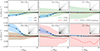 |
Fig. 2. Stacked mean radial profiles in the Planck HFI channels towards 112 CHEX-MATE clusters. Black crosses with error bars show the observed mean SZ signal and its standard uncertainty. The CMB and GTD mean models are shown as solid green and red lines, respectively. The dash-dotted red line marks the dust component after the CTD correction. Solid and dashed blue lines represent the mean rSZ and cSZ models. Shaded areas cover the 16th–84th percentiles intervals. The normalised mean covariance matrices of the observed radial profiles (within 5R500), at each frequency, are shown as inserts. |
For the SZ effect, the relativistic model describes the stacked data towards the cluster centres better than the classical template, reducing the stacked residuals by about 18% within 3R500 (and considering all HFI channels). The results are particularly evident in the 353 GHz and 545 GHz channels, which are closer to the maximum of the SZ effect and where relativistic corrections are expected to be more relevant (see e.g. Appendix B). We note that the residuals are computed by comparing the stacked data with the average of individually fitted SZ models, rather than fitting the stacked profiles themselves. In individual fits, the improvement is less evident (as expected for Planck data), with a median χ2 reduction of about 0.4%.
These differences observed in the SZ signal have an impact on the modelled pressure profiles. In Fig. 3, we show the relative differences in the pressure parameters. In general, slopes are less affected by rSZ corrections (βrSZ/βcSZ − 1 ∼ 0.5%, αrSZ/αcSZ − 1 ∼ 0.8%) than P0 (about 9%). This results in an increase in the pressure profiles, as shown in Fig. 4. From 0.1 to 3R500, the median fractional change spans from  to
to  (with 16th–84th percentile scatter), showing an almost flat behaviour within R500. This trend reflects the joint rSZ and X-ray set-up (inclusion of a temperature profile in the SZ spectra, fixed internal slope and c500, constraining the Planck unresolved inner region with the X-ray data), as well as the residual correlations between P0, α, and β. An example of the marginalised posteriors for the pressure profile parameters is shown in Appendix B (Fig. B.2). In general, the change in pressures is comparable to that estimated by Lee et al. (2020) considering clusters at 5 keV (the average temperature of CHEX-MATE clusters is about 6.9 keV).
 |
Fig. 3. Fractional differences in the pressure profile parameters (from left to right: P0, α, β) between the rSZ and cSZ models. Median (dashed red) and mean (dash-dotted black) are shown with vertical lines and in the legends with 16th–84th percentiles from the reference values. |
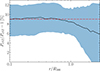 |
Fig. 4. Median fractional change in the pressure profiles between rSZ and cSZ models. The median at 0.1R500 is shown as a visual reference with the dash-dotted red line, while the blue interval encompasses the 16th–84th percentile range. |
4.2. Cluster posteriors and global ηT distribution
With or without rSZ corrections, the posterior distributions of ηT do not show remarkably Gaussian behaviours (with more skewed distributions, as is also noted in Wan et al. 2021), with relative uncertainties of the order of 14%. Generally, we find that lognormal distributions better describe the shape of the posteriors, in agreement with the definition of ηT as a positive quantity, given by the product of independent terms (Eq. (4)). Moreover, an anti-correlation with P0 is present (see Fig. B.2 for an example). Thus, we observe a decrease in ηT, of the same order as P0, when relativistic corrections are included (median ∼8%, see Table 1). The level of the shift is also temperature-dependent, as is shown in Fig. 5. Considering the temperature estimated from the cluster spectra within [0.15, 0.75]R500, we observe a linear correlation (Pearson r statistic: ∼ − 0.7), with fractional differences from about −5% to −14% in the temperature range 3–13 keV, similar to what was found for Compton y by Perrott (2024). However, we note that these shifts are of the same order (or lower) as the actual 1σ confidence interval on ηT. Therefore, it is difficult to assess the impact of the temperature dependence of the rSZ corrections on the final results for single clusters, or, conversely, to probe the cluster temperature from relativistic SZ data alone (as also noted by Perrott 2024).
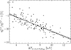 |
Fig. 5. Temperature effect of the relativistic correction on ηT. Uncertainties on ηT values are not shown in the figure, but are at a 14% level. The dashed line (with 1σ confidence interval) shows the trend of the best linear fit to the data. |
Summary of the ηT distribution statistics for the cSZ and rSZ models, Tier-1 and Tier-2 subsamples, the three morphological classes, and the fractional mean and median changes (with 16th–84th percentile variation) given by rSZ corrections and molecular hydrogen fraction in NH.
In Fig. 6, we show the distribution of ηT for the 116 CHEX-MATE clusters with the rSZ model, while in Table 1 we summarise the main statistics of the distribution. In general, it has an asymmetric shape with a more prominent tail towards larger values, as pointed out by the skewness and kurtosis (γ and κ in Table 1). The bulk of the distribution is close to unity (i.e. with the assumption of an ideal ICM distribution with spherical symmetry, no clumps, or bias given in the cosmological framework). Considering the CHEX-MATE subsamples Tier-1 (built to be a local anchor) and Tier-2 (a reference sample for the most massive structures), we do not find strong differences in their ηT distributions. From a Kolmogorov–Smirnov test, we have a p-value of 0.68. Thus, we cannot reject the null hypothesis that the two distributions come from the same underlying ηT population.
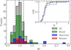 |
Fig. 6. Distributions (and cumulatives in the insert panel) of the ηT parameter for the CHEX-MATE sample (black bins). Red, green, and blue bins define the distribution of the relaxed, mixed, and disturbed clusters, respectively. Dash-dotted vertical lines show the 16th and 84th percentiles, and the dashed line marks the median. |
4.3. Dependence on cluster morphology and physics
The three outlier clusters with ηT > 2 (PSZ2G124.20-36.48, PSZ2G143.26+65.24, and PSZ2G218.81+35.51) are all bimodal systems, as is shown by their X-ray images (see Appendix C). For these systems, assumptions of spherical symmetry and smooth thermodynamical profiles are unlikely to hold, and the limited angular resolution of Planck prevents a clear separation of the structures in the SZ data. These systematics are effectively captured by ηT as discrepancies between the X-ray and SZ profiles. Motivated by this, we examine potential correlations between ηT and cluster properties such as morphology, redshift, mass, and temperature. For the CHEX-MATE project, Campitiello et al. (2022) divided the clusters into three dynamical classes: relaxed, mixed, and disturbed. In Fig. 6 and Table 1, we show the properties of the ηT distributions for these subsamples. Disturbed clusters present a broader distribution and are responsible for the scatter in the ηT right tail. Mixed systems are the majority in the CHEX-MATE sample and drive overall statistical trends. Finally, the relaxed subsample is closer and less scattered around ηT = 1 than the other classes.
Beyond discrete classification, morphology was continuously quantified by Campitiello et al. (2022) with a set of X-ray indicators, collected with a combined parameter ℳ (Rasia et al. 2013; Cialone et al. 2018). Moreover, Benincasa et al. (in prep.) applied for the first time a Zernike Polynomials-based morphological indicator, 𝒞 (introduced in Capalbo et al. 2020, only for SZ images), on the CHEX-MATE X-ray cluster observations to estimate the relaxation parameter χ (Haggar et al. 2020; De Luca et al. 2021). In general, the lower ℳ and 𝒞 are, the more relaxed the cluster is (and the opposite for χ), as shown in the left panels of Fig. 7. No clear trends are present between ηT and these indicators. However, more relaxed clusters (leftmost data points) show less scatter, and in some cases smaller uncertainties, than disturbed ones (rightmost points). This trend is also reflected in the higher skewness and kurtosis (Table 1), as well as in the variation of the 16th–84th percentiles of the sample quartiles (grey intervals in Fig. 7). We note, though, that the CHEX-MATE sample does not collect many relaxed and disturbed systems. Thus, a more detailed study of this trend in ηT (and its impact on cosmological results) could be obtained through hydrodynamical simulations. Regarding any correlation between ηT and the mass, temperature, or redshift of the clusters (right panels of Fig. 7), we find weak or no significant trends. In particular, we have Spearman correlation coefficients of about 0.14 for M500 (p-value = 0.12) and 0.31 for temperature (p = 6.1 ⋅ 10−4).
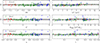 |
Fig. 7. Distribution of ηT values (with 1σ error bars) against cluster morphological indicators ℳ, 𝒞, χ (upper to lower left panels, respectively) and cluster temperatures, masses, and redshifts (right panels). Dynamical classes of Campitiello et al. (2022) are shown as red circles (relaxed), green triangles (mixed), and blue squares (disturbed). Shaded grey envelopes denote the 16th–84th percentile dispersion dividing the sample in quartiles. The x axis in the χ panel is reversed, to preserve the same relaxation ordering of ℳ and 𝒞. |
4.4. Other source of systematics
The Planck SZ data, although highly sensitive, lack the resolution to probe the inner regions of CHEX-MATE clusters. Thus, we jointly fit millimetre and X-ray data, fixing some SZ pressure parameters (Sect. 3.3). Any impact of these fixed parameters on the estimate of ηT is expected to be minor due to the strong constraints from the X-ray profiles, although it cannot be excluded for highly disturbed systems with significant substructures (e.g. the bimodal clusters with ηT > 2). Future improvements can be achieved by including weak lensing data (e.g. as is done in Chappuis et al. 2025; Saxena et al. 2025), ground-based SZ observations at higher resolutions such as SPT and ACT (for CHEX-MATE analyses, see Oppizzi et al. 2023; Gavidia et al. 2025), or with Bolocam, MUSTANG, and NIKA2 (Romero et al. 2015; Adam et al. 2016; Ruppin et al. 2018).
As is detailed in Bourdin et al. (2023), the fraction of molecular hydrogen in the column density must be considered towards the CHEX-MATE clusters for accurate estimates of X-ray spectra, especially for clusters closer to the galactic plane. To assess the impact of the molecular fraction, we repeated the analysis considering only the atomic component. In general, a lower NH yields higher X-ray spectroscopic temperatures and slightly lower emission measures. We then expect (from Eq. (16)) an increase in ηT, since temperature estimates are more sensitive to absorption model variations. This effect is shown in the left panel of Fig. 8 and summarised in Table 1. A change is observed, with a median (mean) variation of about 1% (2.7%), but reaching values up to 34% for some clusters. This small variation reflects the selection of CHEX-MATE clusters. Most of them (about 80% of the total) are in regions where the molecular content is negligible, or its contribution is lower than 10% on average, as shown by Bourdin et al. (2023). Moreover, residual contamination from Galactic dust emission can introduce systematics in our analysis. As in Wan et al. (2021), we tested the robustness of our results by checking for ηT correlations with the distance from the Galactic plane, as shown in the right panel of Fig. 8. If the contamination were significant, clusters closer to the Galactic plane would be more affected. However, no significant trend is observed.
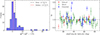 |
Fig. 8. Left panel: Fractional change in ηT when using the atomic column density in the X-ray analysis. Vertical lines show the median (red) and mean (black) values. Right panel: Correlation of ηT with the cluster angular distance from the Galactic plane. The dash-dotted line shows the ηT = 1 line as a visual reference. Relaxed, mixed, and disturbed clusters are shown as red circles, green triangles, and blue squares, respectively. |
As a final consideration, we note that current X-ray telescopes, such as Chandra, XMM-Newton, and even eROSITA exhibit systematic discrepancies in the spectroscopic temperatures (e.g. see Nevalainen et al. 2010; Schellenberger et al. 2015; Migkas et al. 2024). Moreover, these discrepancies are temperature-dependent, with larger deviations at higher temperatures. Thus, ηT values measured with different telescopes are expected to differ, with XMM-Newton generally yielding lower values compared to Chandra, as also shown in B17. The mean ηT value of 1.01 ± 0.03 (standard error) for the CHEX-MATE clusters denotes good agreement between XMM-Newton temperatures and millimetre estimates (and, in particular, for the relaxed subsample where biases are expected to be smaller). However, a detailed description of the cross-calibration issues and their impact on the values of ηT is beyond the scope of this work, based on a follow-up of Planck-selected clusters observed with XMM-Newton.
5. Discussion and conclusions
In this work, we present a new study of systematic mismatches in temperature estimates derived from a joint analysis of XMM-Newton and Planck-HFI observations. Discrepancies between X-ray and millimetre estimates are expected, as the usual simplifying assumptions for the ICM distribution (e.g. spherical symmetry, and regular profiles) only approximate the gas distribution. Thus, these mismatches can be used to improve cosmological constraints, our knowledge of the cluster structure, or to cross-calibrate temperature measurements (K19; Ettori et al. 2020; Wan et al. 2021). Compared to previous studies, this work extends the analysis to a larger sample of 116 galaxy clusters from the PSZ2 catalogue, selected for the CHEX-MATE project to study the local cluster population (Tier-1 subsample) and (Tier-2) massive systems (CHEX-MATE Collaboration 2021). In particular, we improve the parametric methodology of B17 including a more detailed X-ray characterisation of SP contamination, the molecular fraction in the hydrogen column density (as estimated in Bourdin et al. 2023), and relativistic corrections in the SZ modelling, based on X-ray temperatures. Our findings can be summarised as follows.
When relativistic corrections are included, the residuals within 3R500 in the mean stacked profiles (Fig. 2) are reduced by approximately 18%. In addition, the pressure profiles (Fig. 4) show a noteworthy fractional increase of about 8%, with a gradient from 0.1R500 (median value and 16th–84th dispersion:  ) to 3R500 (
 ). Thus, given the anti-correlation between the normalisation of the pressure profiles and ηT, we find a similar change for ηT, on average of
  (median: −8.3%). The shift depends on the cluster temperature, ranging from about −5% to −14% over the 3–13 keV interval. These changes in ηT (if we consider these as systematic biases in Compton y) are similar to those found in previous studies, such as in Lee et al. (2020) and Perrott (2024). However, in individual cluster fits, the relativistic model is only marginally favoured, and the relative uncertainties in ηT (about 14%) are too large to constrain temperatures from relativistic SZ spectra. The inclusion of the molecular content in the X-ray absorption model is crucial for accurate temperature estimates (Bourdin et al. 2023). If not considered, we observe for the CHEX-MATE sample a mean shift on ηT (and thus on X-ray temperatures) of
  (median: 1%, but it could be up to 34% for some cluster).
We find little or no correlation between ηT and cluster masses, redshifts, and temperatures (Fig. 7). Moreover, we do not observe relevant differences between the ηT distributions of Tier-1 and Tier-2 subsamples. Considering the CHEX-MATE morphology studied in Campitiello et al. (2022) and Benincasa et al. (in prep.), the dynamical state of the clusters mainly affects the scatter of ηT values (Table 1 and Fig. 6). The CHEX-MATE ηT distribution has a mean of 1.01 ± 0.03 (median 0.97) and is positively skewed, with relaxed clusters having values closer to unity and less scattered than mixed and disturbed systems, prevalent in the right tail. Thus, samples with less relaxed systems are prone to present more outliers that, if unaccounted for, can bias subsequent analyses such as cosmological constraints (K19). Based on these results, we shall use a large sample of simulated clusters to extend the investigation of the relation between ηT and the cluster dynamical state. The information derived from the simulations, in combination with the results of this work, will then be used to derive new cosmological constraints on H0 extending the methodology of K19.
Acknowledgments
We thank the anonymous referee for useful comments. HB, FDL, SE, PM, MR, MS acknowledge the financial contribution from the contracts Prin-MUR 2022 supported by Next Generation EU (M4.C2.1.1, n.20227RNLY3 The concordance cosmological model: stress-tests with galaxy clusters), MDP from PRIN-MUR grant 20228B938N “Mass and selection biases of galaxy clusters: a multi-probe approach” funded by the European Union Next generation EU, Mission 4 Component 1 CUP C53D2300092 0006, MS from contract INAF mainstream project 1.05.01.86.10 and INAF Theory Grant 2023: Gravitational lensing detection of matter distribution at galaxy cluster boundaries and beyond (1.05.23.06.17), LL from the INAF grant 1.05.12.04.01. HB, FDL, PM also acknowledge the support by the Fondazione ICSC, Spoke 3 Astrophysics and Cosmos Observations, National Recovery and Resilience Plan (Piano Nazionale di Ripresa e Resilienza, PNRR) Project ID CN_00000013 “Italian Research Center on High-Performance Computing, Big Data and Quantum Computing” funded by MUR Missione 4 Componente 2 Investimento 1.4: Potenziamento strutture di ricerca e creazione di “campioni nazionali di R&S (M4C2-19 )” – Next Generation EU (NGEU), and by INFN through the InDark initiative, M.M.E. and E.P. the support of the French Agence Nationale de la Recherche (ANR), under grant ANR-22-CE31-0010, M.G. from the ERC Consolidator Grant BlackHoleWeather (101086804), DE from the Swiss National Science Foundation (SNSF) under grant agreement 200021_212576, BJM from Science and Technology Facilities Council grants ST/V000454/1 and ST/Y002008/1. H.S and J.S. were supported by NASA Astrophysics Data Analysis Program (ADAP) Grant 80NSSC21K1571. AF acknowledges the project “Strengthening the Italian Leadership in ELT and SKA (STILES)”, proposal nr. IR0000034, admitted and eligible for funding from the funds referred to in the D.D. prot. no. 245 of August 10, 2022 and D.D. 326 of August 30, 2022, funded under the program “Next Generation EU” of the European Union, “Piano Nazionale di Ripresa e Resilienza” (PNRR) of the Italian Ministry of University and Research (MUR), “Fund for the creation of an integrated system of research and innovation infrastructures”, Action 3.1.1 “Creation of new IR or strengthening of existing IR involved in the Horizon Europe Scientific Excellence objectives and the establishment of networks”. This research was supported by the International Space Science Institute (ISSI) in Bern, through ISSI International Team project #565 (Multi-Wavelength Studies of the Culmination of Structure Formation in the Universe), the Basic Science Research Program through the National Research Foundation of Korea (NRF) funded by the Ministry of Education (2019R1A6A1A10073887), the 2025 KAIST-U.S. Joint Research Collaboration Open Track Project for Early-Career Researchers, supported by the International Office at the Korea Advanced Institute of Science and Technology (KAIST). Work at Argonne National Lab is supported by UChicago Argonne LLC, Operator of Argonne National Laboratory (Argonne). Argonne, a U.S. Department of Energy Office of Science Laboratory, is operated under contract no. DE-AC02-06CH11357. FDL, HB, and PM also thank the INFN Roma2 IT group for their invaluable support, particularly in the aftermath of the recent fire at their facilities. This work made use of IDL Astronomy Users’s Library (Landsman 1993), HEASoft (Nasa High Energy Astrophysics Science Archive Research Center (Heasarc) 2014), HEALPix (Górski et al. 2005; Zonca et al. 2019) and diverse PYTHON packages: NUMPY (Harris et al. 2020), SCIPY (Virtanen et al. 2020), MATPLOTLIB (Hunter 2007), SEABORN (Waskom 2021), PANDAS (McKinney 2010; Pandas development team 2020), ASTROPY (Astropy Collaboration 2013, 2018, 2022).
References
- Adam, R., Comis, B., Bartalucci, I., et al. 2016, A&A, 586, A122 [NASA ADS] [CrossRef] [EDP Sciences] [Google Scholar]
- Adam, R., Arnaud, M., Bartalucci, I., et al. 2017a, A&A, 606, A64 [NASA ADS] [CrossRef] [EDP Sciences] [Google Scholar]
- Adam, R., Bartalucci, I., Pratt, G. W., et al. 2017b, A&A, 598, A115 [NASA ADS] [CrossRef] [EDP Sciences] [Google Scholar]
- Allen, S. W., Evrard, A. E., & Mantz, A. B. 2011, ARA&A, 49, 409 [Google Scholar]
- Ansarifard, S., Rasia, E., Biffi, V., et al. 2020, A&A, 634, A113 [NASA ADS] [CrossRef] [EDP Sciences] [Google Scholar]
- Arnaud, M., Pratt, G. W., Piffaretti, R., et al. 2010, A&A, 517, A92 [CrossRef] [EDP Sciences] [Google Scholar]
- Asplund, M., Grevesse, N., Sauval, A. J., & Scott, P. 2009, ARA&A, 47, 481 [NASA ADS] [CrossRef] [Google Scholar]
- Astropy Collaboration (Robitaille, T. P., et al.) 2013, A&A, 558, A33 [NASA ADS] [CrossRef] [EDP Sciences] [Google Scholar]
- Astropy Collaboration (Price-Whelan, A. M., et al.) 2018, AJ, 156, 123 [Google Scholar]
- Astropy Collaboration (Price-Whelan, A. M., et al.) 2022, ApJ, 935, 167 [NASA ADS] [CrossRef] [Google Scholar]
- Balboni, M., Ettori, S., Gastaldello, F., et al. 2025, A&A, 695, A180 [NASA ADS] [CrossRef] [EDP Sciences] [Google Scholar]
- Bartalucci, I., Molendi, S., Rasia, E., et al. 2023, A&A, 674, A179 [NASA ADS] [CrossRef] [EDP Sciences] [Google Scholar]
- Bertin, E., & Arnouts, S. 1996, A&AS, 117, 393 [NASA ADS] [CrossRef] [EDP Sciences] [Google Scholar]
- Birkinshaw, M. 1999, Phys. Rep., 310, 97 [Google Scholar]
- Böhringer, H., & Werner, N. 2010, A&ARv, 18, 127 [Google Scholar]
- Bourdin, H., & Mazzotta, P. 2008, A&A, 479, 307 [NASA ADS] [CrossRef] [EDP Sciences] [Google Scholar]
- Bourdin, H., Mazzotta, P., Markevitch, M., Giacintucci, S., & Brunetti, G. 2013, ApJ, 764, 82 [Google Scholar]
- Bourdin, H., Mazzotta, P., Kozmanyan, A., Jones, C., & Vikhlinin, A. 2017, ApJ, 843, 72 [Google Scholar]
- Bourdin, H., De Luca, F., Mazzotta, P., et al. 2023, A&A, 678, A181 [NASA ADS] [CrossRef] [EDP Sciences] [Google Scholar]
- Brunetti, G., & Jones, T. W. 2014, Int. J. Mod. Phys. D, 23, 1430007 [Google Scholar]
- Brunetti, G., Cassano, R., Dolag, K., & Setti, G. 2009, A&A, 507, 661 [NASA ADS] [CrossRef] [EDP Sciences] [Google Scholar]
- Campitiello, M. G., Ettori, S., Lovisari, L., et al. 2022, A&A, 665, A117 [NASA ADS] [CrossRef] [EDP Sciences] [Google Scholar]
- Capalbo, V., De Petris, M., De Luca, F., et al. 2020, MNRAS, 503, 6155 [Google Scholar]
- Carlstrom, J. E., Holder, G. P., & Reese, E. D. 2002, ARA&A, 40, 643 [Google Scholar]
- Cavaliere, A., & Fusco-Femiano, R. 1976, A&A, 49, 137 [NASA ADS] [Google Scholar]
- Cavaliere, A., & Fusco-Femiano, R. 1978, A&A, 70, 677 [NASA ADS] [Google Scholar]
- Cavaliere, A., Danese, L., & De Zotti, G. 1979, A&A, 75, 322 [Google Scholar]
- Challinor, A., & Lasenby, A. 1998, ApJ, 499, 1 [Google Scholar]
- Chappuis, L., Eckert, D., Sereno, M., et al. 2025, A&A, 699, A141 [NASA ADS] [CrossRef] [EDP Sciences] [Google Scholar]
- CHEX-MATE Collaboration (Arnaud, M., et al.) 2021, A&A, 650, A104 [NASA ADS] [CrossRef] [EDP Sciences] [Google Scholar]
- Chiu, I., Mohr, J. J., McDonald, M., et al. 2018, MNRAS, 478, 3072 [Google Scholar]
- Chluba, J., Nagai, D., Sazonov, S., & Nelson, K. 2012, MNRAS, 426, 510 [Google Scholar]
- Chluba, J., Switzer, E., Nelson, K., & Nagai, D. 2013, MNRAS, 430, 3054 [NASA ADS] [CrossRef] [Google Scholar]
- Cialone, G., De Petris, M., Sembolini, F., et al. 2018, MNRAS, 477, 139 [Google Scholar]
- Costanzi, M., Saro, A., Bocquet, S., et al. 2021, Phys. Rev. D, 103, 043522 [Google Scholar]
- Coulton, W. R., Duivenvoorden, A. J., Atkins, Z., et al. 2024, ArXiv e-prints [arXiv:2410.19046] [Google Scholar]
- Cowie, L. L., & Perrenod, S. C. 1978, ApJ, 219, 354 [Google Scholar]
- De Luca, A., & Molendi, S. 2004, A&A, 419, 837 [NASA ADS] [CrossRef] [EDP Sciences] [Google Scholar]
- De Luca, F., De Petris, M., Yepes, G., et al. 2021, MNRAS, 504, 5383 [NASA ADS] [CrossRef] [Google Scholar]
- Donoho, D. 1995, IEEE Trans. Inf. Theory, 41, 613 [CrossRef] [Google Scholar]
- Eckert, D., Ghirardini, V., Ettori, S., et al. 2019, A&A, 621, A40 [NASA ADS] [CrossRef] [EDP Sciences] [Google Scholar]
- Erler, J., Basu, K., Chluba, J., & Bertoldi, F. 2018, MNRAS, 476, 3360 [Google Scholar]
- Ettori, S., Ghirardini, V., & Eckert, D. 2020, Astron. Nachr., 341, 210 [NASA ADS] [CrossRef] [Google Scholar]
- Finkbeiner, D. P., Davis, M., & Schlegel, D. J. 1999, ApJ, 524, 867 [NASA ADS] [CrossRef] [Google Scholar]
- Fioretti, V., Mineo, T., Lotti, S., et al. 2024, A&A, 691, A229 [NASA ADS] [CrossRef] [EDP Sciences] [Google Scholar]
- Gaspari, M., Churazov, E., Nagai, D., Lau, E. T., & Zhuravleva, I. 2014, A&A, 569, A67 [NASA ADS] [CrossRef] [EDP Sciences] [Google Scholar]
- Gastaldello, F., Marelli, M., Molendi, S., et al. 2022, ApJ, 928, 168 [NASA ADS] [CrossRef] [Google Scholar]
- Gavidia, A., Kim, J., Sayers, J., et al. 2025, A&A, submitted [arXiv:2507.10857] [Google Scholar]
- Ghirardini, V., Ettori, S., Eckert, D., et al. 2018, A&A, 614, A7 [NASA ADS] [CrossRef] [EDP Sciences] [Google Scholar]
- Ghirardini, V., Eckert, D., Ettori, S., et al. 2019, A&A, 621, A41 [NASA ADS] [CrossRef] [EDP Sciences] [Google Scholar]
- Ghirardini, V., Bulbul, E., Artis, E., et al. 2024, A&A, 689, A298 [NASA ADS] [CrossRef] [EDP Sciences] [Google Scholar]
- Ghizzardi, S. 2001, In Flight Calibration of the PSF for the MOS1 and MOS2 Cameras, Tech. rep., XMM-Newton Calibration Documentation (XMM-SOC-CAL-TN-0022) [Google Scholar]
- Ghizzardi, S. 2002, In Flight Calibration of the PSF for the PN Camera, Tech. rep., XMM-Newton Calibration Documentation (XMM-SOC-CAL-TN-0029) [Google Scholar]
- Gianfagna, G., De Petris, M., Yepes, G., et al. 2021, MNRAS, 502, 5115 [NASA ADS] [CrossRef] [Google Scholar]
- Gonzalez, A. H., Sivanandam, S., Zabludoff, A. I., & Zaritsky, D. 2013, ApJ, 778, 14 [Google Scholar]
- Górski, K. M., Hivon, E., Banday, A. J., et al. 2005, ApJ, 622, 759 [Google Scholar]
- Haggar, R., Gray, M. E., Pearce, F. R., et al. 2020, MNRAS, 492, 6074 [NASA ADS] [CrossRef] [Google Scholar]
- Harris, C. R., Millman, K. J., van der Walt, S. J., et al. 2020, Nature, 585, 357 [NASA ADS] [CrossRef] [Google Scholar]
- Hunter, J. D. 2007, Comput. Sci. Eng., 9, 90 [NASA ADS] [CrossRef] [Google Scholar]
- Hurier, G. 2016, A&A, 596, A61 [NASA ADS] [CrossRef] [EDP Sciences] [Google Scholar]
- Itoh, N., Kohyama, Y., & Nozawa, S. 1998, ApJ, 502, 7 [Google Scholar]
- Katayama, H., Takahashi, I., Ikebe, Y., Matsushita, K., & Freyberg, M. J. 2004, A&A, 414, 767 [NASA ADS] [CrossRef] [EDP Sciences] [Google Scholar]
- Kay, S. T., Braspenning, J., Chluba, J., et al. 2024, MNRAS, 534, 251 [Google Scholar]
- Kim, J., Sayers, J., Sereno, M., et al. 2024, A&A, 686, A97 [NASA ADS] [CrossRef] [EDP Sciences] [Google Scholar]
- Kitayama, T., Komatsu, E., Ota, N., et al. 2004, PASJ, 56, 17 [NASA ADS] [Google Scholar]
- Kompaneets, A. S. 1957, JEPT, 4, 730 [Google Scholar]
- Kozmanyan, A., Bourdin, H., Mazzotta, P., Rasia, E., & Sereno, M. 2019, A&A, 621, A34 [NASA ADS] [CrossRef] [EDP Sciences] [Google Scholar]
- Kravtsov, A. V., & Borgani, S. 2012, ARA&A, 50, 353 [Google Scholar]
- Kuhn, L., Li, Z., & Coulton, W. R. 2025, ArXiv e-prints [arXiv:2504.18637] [Google Scholar]
- Kuntz, K. D., & Snowden, S. L. 2000, ApJ, 543, 195 [Google Scholar]
- Kuntz, K. D., & Snowden, S. L. 2008, A&A, 478, 575 [NASA ADS] [CrossRef] [EDP Sciences] [Google Scholar]
- Landsman, W. B. 1993, The IDL Astronomy User’s Library, ASP Conf. Ser., 52, 246 [Google Scholar]
- Leccardi, A., & Molendi, S. 2008, A&A, 486, 359 [NASA ADS] [CrossRef] [EDP Sciences] [Google Scholar]
- Lee, E., Chluba, J., Kay, S. T., & Barnes, D. J. 2020, MNRAS, 493, 3274 [Google Scholar]
- Lovisari, L., & Reiprich, T. H. 2019, MNRAS, 483, 540 [Google Scholar]
- Lumb, D. H., Warwick, R. S., Page, M., & De Luca, A. 2002, A&A, 389, 93 [CrossRef] [EDP Sciences] [Google Scholar]
- Luzzi, G., D’Angelo, E., Bourdin, H., et al. 2022, EPJ Web Conf., 257, 00028 [Google Scholar]
- Marelli, M., Molendi, S., Rossetti, M., et al. 2021, ApJ, 908, 37 [CrossRef] [Google Scholar]
- Markwardt, C. B. 2009, ASP Conf. Ser., 411, 251 [Google Scholar]
- Mastromarino, C., Oppizzi, F., De Luca, F., Bourdin, H., & Mazzotta, P. 2024, A&A, 688, A76 [NASA ADS] [CrossRef] [EDP Sciences] [Google Scholar]
- Mazzotta, P., Rasia, E., Moscardini, L., & Tormen, G. 2004, MNRAS, 354, 10 [NASA ADS] [CrossRef] [Google Scholar]
- McDonald, M., McNamara, B. R., Voit, G. M., et al. 2019, ApJ, 885, 63 [NASA ADS] [CrossRef] [Google Scholar]
- McKinney, W. 2010, in Proceedings of the 9th Python in Science Conference, eds. S. van der Walt, & J. Millman, 56 [Google Scholar]
- Meisner, A. M., & Finkbeiner, D. P. 2014, ApJ, 798, 88 [NASA ADS] [CrossRef] [Google Scholar]
- Melin, J.-B., Bartlett, J. G., & Delabrouille, J. 2006, A&A, 459, 341 [NASA ADS] [CrossRef] [EDP Sciences] [Google Scholar]
- Migkas, K., Kox, D., Schellenberger, G., et al. 2024, A&A, 688, A107 [NASA ADS] [CrossRef] [EDP Sciences] [Google Scholar]
- Mineo, T., Fioretti, V., Lotti, S., et al. 2024, A&A, 691, A230 [NASA ADS] [CrossRef] [EDP Sciences] [Google Scholar]
- Mitchell, R. J., Culhane, J. L., Davison, P. J. N., & Ives, J. C. 1976, MNRAS, 175, 29P [CrossRef] [Google Scholar]
- Mroczkowski, T., Nagai, D., Basu, K., et al. 2019, Space Sci. Rev., 215, 17 [Google Scholar]
- Muñoz-Echeverría, M., Pointecouteau, E., Pratt, G. W., et al. 2025, A&A, 704, A302 [Google Scholar]
- Nagai, D., Kravtsov, A. V., & Vikhlinin, A. 2007, ApJ, 668, 1 [Google Scholar]
- Nasa High Energy Astrophysics Science Archive Research Center (Heasarc). 2014, Astrophysics Source Code Library [record ascl:1408.004] [Google Scholar]
- Navarro, J. F., Frenk, C. S., & White, S. D. M. 1997, ApJ, 490, 493 [Google Scholar]
- Nevalainen, J., David, L., & Guainazzi, M. 2010, A&A, 523, A22 [NASA ADS] [CrossRef] [EDP Sciences] [Google Scholar]
- Nozawa, S., Itoh, N., & Kohyama, Y. 1998, ApJ, 508, 17 [Google Scholar]
- Nozawa, S., Itoh, N., Suda, Y., & Ohhata, Y. 2006, Nuovo Cimento B Ser., 121, 487 [Google Scholar]
- Oppizzi, F., De Luca, F., Bourdin, H., et al. 2023, A&A, 672, A156 [NASA ADS] [CrossRef] [EDP Sciences] [Google Scholar]
- Pacaud, F., Pierre, M., Melin, J.-B., et al. 2018, A&A, 620, A10 [NASA ADS] [CrossRef] [EDP Sciences] [Google Scholar]
- Pandas development team. 2020, https://doi.org/10.5281/zenodo.3509134 [Google Scholar]
- Pearce, F. A., Kay, S. T., Barnes, D. J., Bower, R. G., & Schaller, M. 2019, MNRAS, 491, 1622 [Google Scholar]
- Perrott, Y. 2024, PASA, 41, e087 [Google Scholar]
- Planck Collaboration XXIX. 2014, A&A, 571, A29 [NASA ADS] [CrossRef] [EDP Sciences] [Google Scholar]
- Planck Collaboration I. 2016, A&A, 594, A1 [NASA ADS] [CrossRef] [EDP Sciences] [Google Scholar]
- Planck Collaboration VII. 2016, A&A, 594, A7 [NASA ADS] [CrossRef] [EDP Sciences] [Google Scholar]
- Planck Collaboration XXIII. 2016, A&A, 594, A23 [NASA ADS] [CrossRef] [EDP Sciences] [Google Scholar]
- Planck Collaboration XXIV. 2016, A&A, 594, A24 [NASA ADS] [CrossRef] [EDP Sciences] [Google Scholar]
- Planck Collaboration XXVI. 2016, A&A, 594, A26 [NASA ADS] [CrossRef] [EDP Sciences] [Google Scholar]
- Planck Collaboration XXVII. 2016, A&A, 594, A27 [NASA ADS] [CrossRef] [EDP Sciences] [Google Scholar]
- Planck Collaboration XXXVII. 2016, A&A, 586, A140 [NASA ADS] [CrossRef] [EDP Sciences] [Google Scholar]
- Planck Collaboration XLIII. 2016, A&A, 596, A104 [NASA ADS] [CrossRef] [EDP Sciences] [Google Scholar]
- Planck Collaboration VI. 2020, A&A, 641, A6 [NASA ADS] [CrossRef] [EDP Sciences] [Google Scholar]
- Pointecouteau, E., Giard, M., & Barret, D. 1998, A&A, 336, 44 [NASA ADS] [Google Scholar]
- Pointecouteau, E., Hattori, M., Neumann, D., et al. 2002, A&A, 387, 56 [NASA ADS] [CrossRef] [EDP Sciences] [Google Scholar]
- Pointecouteau, E., Santiago-Bautista, I., Douspis, M., et al. 2021, A&A, 651, A73 [NASA ADS] [CrossRef] [EDP Sciences] [Google Scholar]
- Pratt, G. W., Arnaud, M., Biviano, A., et al. 2019, Space Sci. Rev., 215, 25 [Google Scholar]
- Prokhorov, D. A., & Colafrancesco, S. 2012, MNRAS, 424, L49 [Google Scholar]
- Rasia, E., Meneghetti, M., & Ettori, S. 2013, Astron. Rev., 8, 40 [Google Scholar]
- Reese, E. D., Mohr, J. J., Carlstrom, J. E., et al. 2000, ApJ, 533, 38 [Google Scholar]
- Reese, E. D., Carlstrom, J. E., Joy, M., et al. 2002, ApJ, 581, 53 [NASA ADS] [CrossRef] [Google Scholar]
- Remazeilles, M., & Chluba, J. 2025, MNRAS, 538, 1576 [Google Scholar]
- Remazeilles, M., Bolliet, B., Rotti, A., & Chluba, J. 2018, MNRAS, 483, 3459 [Google Scholar]
- Rephaeli, Y. 1995a, ARA&A, 33, 541 [NASA ADS] [CrossRef] [Google Scholar]
- Rephaeli, Y. 1995b, ApJ, 445, 33 [Google Scholar]
- Romero, C. E., Mason, B. S., Sayers, J., et al. 2015, ApJ, 807, 121 [Google Scholar]
- Rossetti, M., Eckert, D., Gastaldello, F., et al. 2024, A&A, 686, A68 [NASA ADS] [CrossRef] [EDP Sciences] [Google Scholar]
- Ruppin, F., Mayet, F., Pratt, G., et al. 2018, A&A, 615, A112 [NASA ADS] [CrossRef] [EDP Sciences] [Google Scholar]
- Salvetti, D., Marelli, M., Gastaldello, F., et al. 2017, Exp. Astron., 44, 309 [Google Scholar]
- Sarazin, C. L. 1986, Rev. Mod. Phys., 58, 1 [Google Scholar]
- Saxena, H., Sayers, J., Gavidia, A., et al. 2025, A&A, 700, A128 [NASA ADS] [CrossRef] [EDP Sciences] [Google Scholar]
- Sayers, J., Montaña, A., Mroczkowski, T., et al. 2019, ApJ, 880, 45 [Google Scholar]
- Schellenberger, G., Reiprich, T. H., Lovisari, L., Nevalainen, J., & David, L. 2015, A&A, 575, A30 [NASA ADS] [CrossRef] [EDP Sciences] [Google Scholar]
- Schellenberger, G., Giacintucci, S., Lovisari, L., et al. 2022, ApJ, 925, 91 [NASA ADS] [CrossRef] [Google Scholar]
- Sereno, M., Umetsu, K., Ettori, S., et al. 2018, ApJ, 860, L4 [NASA ADS] [CrossRef] [Google Scholar]
- Serlemitsos, P. J., Smith, B. W., Boldt, E. A., Holt, S. S., & Swank, J. H. 1977, ApJ, 211, L63 [NASA ADS] [CrossRef] [Google Scholar]
- Silk, J., & White, S. D. M. 1978, ApJ, 226, L103 [Google Scholar]
- Smith, R. K., Brickhouse, N. S., Liedahl, D. A., & Raymond, J. C. 2001, ApJ, 556, L91 [Google Scholar]
- Snowden, S. L., Mushotzky, R. F., Kuntz, K. D., & Davis, D. S. 2008, A&A, 478, 615 [NASA ADS] [CrossRef] [EDP Sciences] [Google Scholar]
- Starck, J. L., Pantin, E., & Murtagh, F. 2002, PASP, 114, 1051 [NASA ADS] [CrossRef] [Google Scholar]
- Starck, J.-L., Fadili, J., & Murtagh, F. 2007, IEEE Trans. Image Process., 16, 297 [Google Scholar]
- Starck, J.-L., Fadili, J. M., Digel, S., Zhang, B., & Chiang, J. 2009, A&A, 504, 641 [NASA ADS] [CrossRef] [EDP Sciences] [Google Scholar]
- Strüder, L., Briel, U., Dennerl, K., et al. 2001, A&A, 365, L18 [Google Scholar]
- Sunyaev, R. A., & Zeldovich, Y. B. 1972, Com. Ap&SS, 4, 173 [Google Scholar]
- Sunyaev, R. A., & Zeldovich, I. B. 1980, ARA&A, 18, 537 [Google Scholar]
- Tozzi, P., Gastaldello, F., Molendi, S., et al. 2015, A&A, 580, A6 [NASA ADS] [CrossRef] [EDP Sciences] [Google Scholar]
- Turner, M. J. L., Abbey, A., Arnaud, M., et al. 2001, A&A, 365, L27 [CrossRef] [EDP Sciences] [Google Scholar]
- Van Weeren, R. J., De Gasperin, F., Akamatsu, H., et al. 2019, Space Sci. Rev., 215, 16 [NASA ADS] [CrossRef] [Google Scholar]
- Vaughan, B. J., Sayers, J., Spencer, L., et al. 2025, ArXiv e-prints [arXiv:2510.08837] [Google Scholar]
- Verner, D. A., Ferland, G. J., Korista, K. T., & Yakovlev, D. G. 1996, ApJ, 465, 487 [Google Scholar]
- Vikhlinin, A., Kravtsov, A., Forman, W., et al. 2006, ApJ, 640, 691 [Google Scholar]
- Vikhlinin, A., Kravtsov, A. V., Burenin, R. A., et al. 2009, ApJ, 692, 1060 [Google Scholar]
- Virtanen, P., Gommers, R., Oliphant, T. E., et al. 2020, Nat. Methods, 17, 261 [Google Scholar]
- Voit, G. M. 2005, Rev. Mod. Phys., 77, 207 [Google Scholar]
- Wan, J. T., Mantz, A. B., Sayers, J., et al. 2021, MNRAS, 504, 1062 [NASA ADS] [CrossRef] [Google Scholar]
- Waskom, M. L. 2021, J. Open Source Softw., 6, 3021 [CrossRef] [Google Scholar]
- Wright, E. L. 1979, ApJ, 232, 348 [Google Scholar]
- Zonca, A., Singer, L., Lenz, D., et al. 2019, J. Open Source Softw., 4, 1298 [Google Scholar]
If ΣX is expressed in terms of photon fluxes (i.e. without accounting for photon energies, counts cm−2 arcmin−2 sr−1), the redshift dimming factor in Eq. (1) becomes (1 + z)−3 (Reese et al. 2000).
For a given threshold λ and a value of wavelet coefficient d, soft-thresholding is defined as: D(d|λ) = sgn(d)(0, |d|−λ)+ (Donoho 1995).
Appendix A: Comparison with the standard CHEX-MATE pipeline
The results shown in this paper are based on an independent analysis of the CHEX-MATE galaxy cluster sample. This choice was made to extend the already developed cosmological pipeline of K19 to a larger sample of clusters (almost a factor two) and, at the same time, to include more sources of systematics in the model. Differences from the CHEX-MATE standard pipeline mainly concern the X-ray background modelling, including flare filtering and the calibration of the SP component. In Rossetti et al. (2024), the authors conducted an accurate estimate of the SP and QPB components for the background, considering the correlations between the count rates inside and outside the regions subtended by the FOV for the EPIC cameras, similarly to the method of De Luca & Molendi (2004), Leccardi & Molendi (2008), and Ghirardini et al. (2018). In particular, the scaling of the SP component with the IN-OUT method from Ghirardini et al. (2018) is extended to spectral analysis, and uncertainties in the background model are propagated to cluster spectra (e.g. for temperature and metallicity profiles) considering an MCMC fit. For this reason, we tested the consistency between our results and the CHEX-MATE outcomes for 28 clusters of the DR1 subsample presented in Rossetti et al. (2024). For this analysis, we adopted the same radial binning, cluster modelling (e.g. NH, abundance table, cross-sections) and spectral band (0.5–12 keV) used for temperature estimates.
A comparison of the two pipelines is shown in Fig. A.1. In the left panel, we show the direct comparison (with 1σ uncertainties) of the temperature results of this work (kT, x axis) and of the CHEX-MATE pipeline (kTref, y axis), while the right panel presents the radial distribution of their ratio. In general, the temperatures are close to the equality line, and the distribution of their ratio is close to being symmetric and centred on 1. However, the distribution has a non-zero excess kurtosis, with heavier tails than the fitted Gaussian. From the radial profile, the agreement between the two pipelines is stronger towards the cluster centres and at intermediate radii, while the outliers occur mostly in the cluster outskirts (beyond R500), where the S/N is lower and the measures are more challenging. We note, however, that our last bin has edges between 0.8 − 1R500. Therefore, the two pipelines yield consistent temperature estimates in the radial range explored in this work (shown in the figure with the dark blue bins).
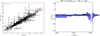 |
Fig. A.1. (Left panel): Comparison between the CHEX-MATE pipeline temperature (Tref) and the results of this work, with 1σ error bars and the equality line in dashed red. (Right panel): Ratios between the temperature estimates (grey dots) as a function of the radial distance from the cluster centres. The overall distribution is shown in the right marginal plot, with a Gaussian fit. Dark blue areas show the 16th–84th percentile range in the radial binning of this work. The bin mean (with its standard uncertainty) and median values are shown with black dots (with error bars) and dashed segments. As a visual reference, the y = 1 line is shown with a dash-dotted line. |
Appendix B: Relativistic correction for thermal SZ effect
In the classical approximation, the tSZ amplitude (i.e. the y; Eqs. 2, 3) depends on the electron pressure (and thus on Te), while the spectrum is independent of the electron temperature. As shown in Fig. B.1, the classical spectrum exhibits a decrement of intensities at lower frequencies and an increment at higher frequencies (due to inverse Compton scattering of CMB photons), with a crossover frequency at around 217 GHz. When relativistic electrons are included, the spectra become temperature-dependent and more asymmetric. For increasing temperatures we generally have a reduction of the peak-to-trough amplitude and a redistribution of the signal towards the Wien tail, with crossover and peak positions shifting towards higher frequencies. As a consequence, classical modelling can lead to biased estimates of the y parameter, with the sign and magnitude depending on the observed frequencies (and the instrumental response). As shown in Fig. B.1 for the HFI bands, the non-relativistic formulation generally overestimates the signal at frequencies below the crossover and near the peak. At higher frequencies (≳480 GHz), we have instead an underestimation. Therefore, for a proper characterisation of the cluster signal (and of the derived thermodynamical information) a proper relativistic treatment is necessary.
Assuming an isothermal distribution for the gas, the tSZ signal, LOS integrated and corrected for relativistic effects, can be written as:
 (B.1)
(B.1)
where 𝒴(x) and Θe are the vectors with the expansion coefficients of Nozawa et al. (1998, 2006) and their associated θe powers, respectively:
![Mathematical equation: $$ \begin{aligned}&\boldsymbol{\mathcal{Y} }(x) = \left[ Y_0(x) , Y_1(x) , Y_2(x) , Y_3(x) , Y_4(x) \right], \end{aligned} $$](/articles/aa/full_html/2026/03/aa57787-25/aa57787-25-eq34.gif) (B.2)
(B.2)
![Mathematical equation: $$ \begin{aligned}&\boldsymbol{\Theta _e}(n_e, \theta _e) = \sigma _T n_e \left[ \theta _e , \theta _e^2 , \theta _e^3 , \theta _e^ 4, \theta _e^5 \right], \end{aligned} $$](/articles/aa/full_html/2026/03/aa57787-25/aa57787-25-eq35.gif) (B.3)
(B.3)
up to the fourth order and where the zeroth order Y0(x) is the Kompaneets solution. With this notation (assuming an isothermal gas), the SZ signal can still be written separating the spatial (Θe) and spectral (𝒴) behaviours. However, the ICM in galaxy clusters is not in an isothermal state and the temperature can vary from cluster cores to the outskirts. To account for LOS temperature variations, we follow a similar approach to Prokhorov & Colafrancesco (2012) and Chluba et al. (2013). Considering Eq. (B.1) as the spectrum given for a reference temperature  along the line of sight, we can introduce corrections for the temperature variation with a second expansion of ISZ around
  :
:
 (B.4)
(B.4)
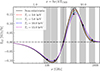 |
Fig. B.1. Comparison between the non-relativistic (solid black line) and relativistic (dashed) tSZ spectra for fixed y = 10−4. The dotted line marks the non-relativistic crossover frequency. Grey intervals show the HFI channels, while arrows mark the direction of the y biases induced by non-relativistic modelling. |
with F(x, θe) and the derivatives defined, respectively, as:
 (B.5)
(B.5)
 (B.6)
(B.6)
As noted in Chluba et al. (2013), the terms  in Eq. (B.4) are equivalent to introduce corrections given by the temperature distribution moments μk about the value
  (along the LOS). Thus, using standardised central moments about the mean, it is possible to simplify Eq. (B.4). For example, considering the first four central moments and defining the reference temperature as the density-weighted temperature, similarly to Prokhorov & Colafrancesco (2012) (or τ-weighted, as in Eq. 15 of Chluba et al. 2013), we have:
 (B.7)
(B.7)
 (B.8)
(B.8)
 (B.9)
(B.9)
Therefore, the first central moment is zero by definition, and the second, third, and fourth are given, respectively, by the temperature variance σe2, skewness γe, and kurtosis κe, all estimated along the LOS. In Eq. (B.8), y(ne, θe) is the Compton y parameter, and it is introduced to replicate the general notation used for the tSZ effect (e.g. Eq. B.1), where it is factorisable as the product of y (which depends on the properties of the gas we are interested in, e.g. the pressure) times a spectrum (with the average gas properties) as in Eq. (12). For the calculation of the relativistic corrections described above, we use the temperature and density functional forms proposed by Vikhlinin et al. (2006), fitted to the X-ray data as described in Sect. 3.1.2. In Fig. B.2, we show an example of the outcome of the MCMC fitting of the rSZ signal for the cluster PSZ2G325.70+17.34.
 |
Fig. B.2. Posterior distributions of the pressure profile parameters for cluster PSZ2G325.70+17.34. Values in captions and dashed black lines report the median, 16th, and 84th percentiles (with plus minus intervals from the median values). Dash-dotted red lines show the position of the maximum likelihood value estimates. |
Appendix C: Galaxy cluster gallery
Fig. C.1 is a gallery of the 118 galaxy clusters of the CHEX-MATE sample. Every image was produced using a sparse denoising algorithm based on a wavelet reconstruction of the maps (Starck et al. 2009; Bourdin et al. 2013). Poisson noise was removed from the images using soft thresholding of B3-spline wavelet transforms, with corrections for the exposure and the vignetting of the XMM-Newton EPIC cameras. The maps were also background subtracted, and all the point sources were masked and inpainted. Each map subtends a region of 2R500 × 2R500, with the X-ray surface brightness extracted in the soft X-ray energy band (0.5–2.5 keV). The maps are shown in logarithmic scale. With respect to the gallery presented in Fig. 6 of CHEX-MATE Collaboration (2021), Fig. C.1 also collects observations not available at that time and considers a different reconstruction and smoothing of the images (e.g. a wavelet reconstruction here, while a Gaussian smoothing in CHEX-MATE Collaboration 2021). The images are ordered according to the combined morphological parameter ℳ (see Table A1 in Campitiello et al. 2022), from the most relaxed to the most disturbed clusters. As discussed in Campitiello et al. (2022), this sample includes a variety of clusters with different dynamical states. In particular, this sample is not dominated by relaxed systems and presents several objects with disturbed morphologies, such as A115 (PSZ2G124.20-36.48), A1430 (PSZ2G143.26+65.24), or PSZ2G218.81+35.51, all with ηT > 2. The clusters excluded from this work are PSZ2G283.91+73.87, affected by the foreground contamination of the Virgo cluster, and PSZ2G028.63+50.15. Both are shown in the gallery with their names in red.
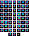 |
Fig. C.1. Wavelet-denoised XMM-Newton images of the 118 CHEX-MATE galaxy clusters, background subtracted and corrected for vignetting and exposure. Surface brightness in the energy range [0.5,25] keV is shown with a logarithmic scale from 0.1 counts per pixel to the image maximum, with point sources removed and inpainted. The maps are centred on the X-ray peak and covers an area of 2R500 × 2R500. |
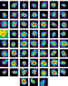 |
Fig. C.1. Continued. |
All Tables
Summary of the ηT distribution statistics for the cSZ and rSZ models, Tier-1 and Tier-2 subsamples, the three morphological classes, and the fractional mean and median changes (with 16th–84th percentile variation) given by rSZ corrections and molecular hydrogen fraction in NH.
All Figures
|
Fig. 1. Mass and redshift distribution of the CHEX-MATE sample (grey). Tier-1 and Tier-2 clusters are shown as red circles and blue triangles, respectively, and common clusters as green squares. Excluded clusters from the analysis are shown with red crosses. |
| In the text | |
|
Fig. 2. Stacked mean radial profiles in the Planck HFI channels towards 112 CHEX-MATE clusters. Black crosses with error bars show the observed mean SZ signal and its standard uncertainty. The CMB and GTD mean models are shown as solid green and red lines, respectively. The dash-dotted red line marks the dust component after the CTD correction. Solid and dashed blue lines represent the mean rSZ and cSZ models. Shaded areas cover the 16th–84th percentiles intervals. The normalised mean covariance matrices of the observed radial profiles (within 5R500), at each frequency, are shown as inserts. |
| In the text | |
|
Fig. 3. Fractional differences in the pressure profile parameters (from left to right: P0, α, β) between the rSZ and cSZ models. Median (dashed red) and mean (dash-dotted black) are shown with vertical lines and in the legends with 16th–84th percentiles from the reference values. |
| In the text | |
|
Fig. 4. Median fractional change in the pressure profiles between rSZ and cSZ models. The median at 0.1R500 is shown as a visual reference with the dash-dotted red line, while the blue interval encompasses the 16th–84th percentile range. |
| In the text | |
|
Fig. 5. Temperature effect of the relativistic correction on ηT. Uncertainties on ηT values are not shown in the figure, but are at a 14% level. The dashed line (with 1σ confidence interval) shows the trend of the best linear fit to the data. |
| In the text | |
|
Fig. 6. Distributions (and cumulatives in the insert panel) of the ηT parameter for the CHEX-MATE sample (black bins). Red, green, and blue bins define the distribution of the relaxed, mixed, and disturbed clusters, respectively. Dash-dotted vertical lines show the 16th and 84th percentiles, and the dashed line marks the median. |
| In the text | |
|
Fig. 7. Distribution of ηT values (with 1σ error bars) against cluster morphological indicators ℳ, 𝒞, χ (upper to lower left panels, respectively) and cluster temperatures, masses, and redshifts (right panels). Dynamical classes of Campitiello et al. (2022) are shown as red circles (relaxed), green triangles (mixed), and blue squares (disturbed). Shaded grey envelopes denote the 16th–84th percentile dispersion dividing the sample in quartiles. The x axis in the χ panel is reversed, to preserve the same relaxation ordering of ℳ and 𝒞. |
| In the text | |
|
Fig. 8. Left panel: Fractional change in ηT when using the atomic column density in the X-ray analysis. Vertical lines show the median (red) and mean (black) values. Right panel: Correlation of ηT with the cluster angular distance from the Galactic plane. The dash-dotted line shows the ηT = 1 line as a visual reference. Relaxed, mixed, and disturbed clusters are shown as red circles, green triangles, and blue squares, respectively. |
| In the text | |
|
Fig. A.1. (Left panel): Comparison between the CHEX-MATE pipeline temperature (Tref) and the results of this work, with 1σ error bars and the equality line in dashed red. (Right panel): Ratios between the temperature estimates (grey dots) as a function of the radial distance from the cluster centres. The overall distribution is shown in the right marginal plot, with a Gaussian fit. Dark blue areas show the 16th–84th percentile range in the radial binning of this work. The bin mean (with its standard uncertainty) and median values are shown with black dots (with error bars) and dashed segments. As a visual reference, the y = 1 line is shown with a dash-dotted line. |
| In the text | |
|
Fig. B.1. Comparison between the non-relativistic (solid black line) and relativistic (dashed) tSZ spectra for fixed y = 10−4. The dotted line marks the non-relativistic crossover frequency. Grey intervals show the HFI channels, while arrows mark the direction of the y biases induced by non-relativistic modelling. |
| In the text | |
|
Fig. B.2. Posterior distributions of the pressure profile parameters for cluster PSZ2G325.70+17.34. Values in captions and dashed black lines report the median, 16th, and 84th percentiles (with plus minus intervals from the median values). Dash-dotted red lines show the position of the maximum likelihood value estimates. |
| In the text | |
|
Fig. C.1. Wavelet-denoised XMM-Newton images of the 118 CHEX-MATE galaxy clusters, background subtracted and corrected for vignetting and exposure. Surface brightness in the energy range [0.5,25] keV is shown with a logarithmic scale from 0.1 counts per pixel to the image maximum, with point sources removed and inpainted. The maps are centred on the X-ray peak and covers an area of 2R500 × 2R500. |
| In the text | |
|
Fig. C.1. Continued. |
| In the text | |
Current usage metrics show cumulative count of Article Views (full-text article views including HTML views, PDF and ePub downloads, according to the available data) and Abstracts Views on Vision4Press platform.
Data correspond to usage on the plateform after 2015. The current usage metrics is available 48-96 hours after online publication and is updated daily on week days.
Initial download of the metrics may take a while.