| Issue |
A&A
Volume 707, March 2026
|
|
|---|---|---|
| Article Number | A315 | |
| Number of page(s) | 13 | |
| Section | Planets, planetary systems, and small bodies | |
| DOI | https://doi.org/10.1051/0004-6361/202558041 | |
| Published online | 24 March 2026 | |
Evidence for stellar contamination and water absorption in NGTS-5b’s transmission spectra with GTC/OSIRIS
1
CAS Key Laboratory of Planetary Sciences, Purple Mountain Observatory, Chinese Academy of Sciences,
Nanjing
210023,
PR China
2
School of Astronomy and Space Science, University of Science and Technology of China,
Hefei
230026,
PR China
3
Instituto de Astrofísica de Canarias (IAC),
Vía Láctea s/n,
38205
La Laguna, Tenerife,
Spain
4
Departamento de Astrofísica, Universidad de La Laguna (ULL),
C/ Padre Herrera,
38206
La Laguna, Tenerife,
Spain
★ Corresponding author: This email address is being protected from spambots. You need JavaScript enabled to view it.
Received:
10
November
2025
Accepted:
16
January
2026
Abstract
Context. Transmission spectroscopy serves as a valuable tool for probing atmospheric absorption features in the terminator regions of exoplanets. Stellar surface heterogeneity can introduce wavelength-dependent contamination that complicates the interpretation of planetary spectra.
Aims. We aim to investigate the atmosphere of the warm sub-Saturn NGTS-5b through optical transmission spectroscopy.
Methods. Two transits were observed with the low-resolution Optical System for Imaging and low-Intermediate-Resolution Integrated Spectroscopy (OSIRIS) on the 10.4 m Gran Telescopio Canarias (GTC). Chromatic transit light curves were modeled to derive optical transmission spectra, and multiple Bayesian spectral retrievals were performed to characterize the atmospheric properties.
Results. Model comparisons provide strong evidence for contamination from unocculted stellar spots. A joint retrieval of the transmission spectra, assuming equilibrium chemistry, indicates a relatively clear atmosphere with a subsolar C/O ratio of <0.22 (90% upper limit) and a low metallicity of 0.10−0.05+0.34× solar solar. Retrievals assuming free chemistry yield strong evidence for the presence of H2O, with its abundance constrained to log XH2O = −0.79−0.17+0.14. However, the abundances of other species remain unconstrained due to limited optical wavelength coverage.
Conclusions. The discrepancies between the two NGTS-5b transit spectra can be attributed to varying levels of stellar contamination. NGTS-5b thus appears to host a relatively clear, water-rich atmosphere, pending confirmation from additional observations of molecular bands in the infrared.
Key words: methods: data analysis / techniques: spectroscopic / planets and satellites: atmospheres / planets and satellites: individual: NGTS-5b
© The Authors 2026
 Open Access article, published by EDP Sciences, under the terms of the Creative Commons Attribution License (https://creativecommons.org/licenses/by/4.0), which permits unrestricted use, distribution, and reproduction in any medium, provided the original work is properly cited.
This article is published in open access under the Subscribe to Open model. This email address is being protected from spambots. You need JavaScript enabled to view it. to support open access publication.
1 Introduction
Transmission spectroscopy (Seager & Sasselov 2000) has been the primary technique for probing absorption and scattering features in exoplanet atmospheres, particularly at the planet’s day-night terminator. To date, precise spectroscopic measurements have been obtained for over 200 exoplanets1, with a primary focus on close-in giant worlds. Water has been detected in nearly half of these atmospheres (Madhusudhan 2019), making it a key tracer for atmospheric composition and chemical processes.
The launch of the James Webb Space Telescope (JWST) in 2021 has enabled mid-infrared observations with unprecedented sensitivity, allowing the identification of a range of key molecules in exoplanet atmospheres, such as H2O, CH4, CO2, SO2, and H2S (e.g., Rustamkulov et al. 2023; Bell et al. 2023; Dyrek et al. 2024; Powell et al. 2024; Kirk et al. 2025). However, JWST offers limited coverage at blue-optical wavelengths, where scattering slopes and pressure-broadened sodium lines are most prominent (Nikolov et al. 2018; Radica et al. 2023). Complementary observations from large ground-based telescopes are therefore essential to provide crucial constraints on stellar contamination and atmospheric properties.
Interpreting transmission spectra requires a thorough understanding of the wavelength-dependent brightness of the host star. However, stellar magnetic activity, in the form of spots (cooler, darker regions; for details, see review by Solanki 2003) and faculae (hotter, brighter regions; see review by Unruh et al. 1999), can produce surface heterogeneity across the stellar disk. When these active regions are occulted by the transiting planet, they can imprint detectable anomalies in the light curve (e.g., Barros et al. 2013; Mohler-Fischer et al. 2013; Kirk et al. 2016; Baluev et al. 2021; Libby-Roberts et al. 2023). In addition, unocculted active regions can bias transmission spectra by altering the baseline stellar flux (e.g., Rackham et al. 2017; Jiang et al. 2021; Lim et al. 2023; Moran et al. 2023; Banerjee et al. 2024), which is commonly referred to as the transit light source (TLS) effect (Apai et al. 2018).
NGTS-5b is a warm sub-Saturn planet with a mass of ∼0.229 MJup, a radius of ∼1.136 RJup, and an equilibrium temperature of ∼952 K (Eigmüller et al. 2019). It orbits its host star with a period of ∼3.357 days, placing it at the upper boundary of the sub-Jovian desert (Szabó & Kiss 2011). The host star is a K2-type dwarf with a mass of ∼0.661 M⊙, a radius of ∼0.739 R⊙, an effective temperature of ∼4987 K, and a metallicity of ∼0.12 dex. Notably, a photometric survey targeting the metastable helium triplet at 10 830 Å with Palomar/WIRC tentatively detected absorption signals from NGTS-5b, highlighting it as a promising candidate for investigating atmospheric escape processes and for assessing the influence of stellar activities (Vissapragada et al. 2022).
In this study, we present the first optical transmission spectroscopy of NGTS-5b, based on two transit observations obtained with the Optical System for Imaging and low-Intermediate-Resolution Integrated Spectroscopy (OSIRIS; Cepa et al. 2000) on the 10.4 m Gran Telescopio CANARIAS (GTC). Our primary aim is to characterize the planet’s atmospheric properties by identifying absorption and scattering features in its optical transmission spectrum.
This paper is structured as follows. Section 2 summarizes the observations and data reduction procedures. Section 3 presents the analysis of the transit light curves. In Section 4, we perform atmospheric retrievals and interpret the resulting transmission spectra. Section 5 discusses possible alternative interpretations and compares our findings with those for similar exoplanets. Finally, Section 6 summarizes our conclusions.
2 Observations and data reduction
2.1 GTC/OSIRIS transit spectroscopy
We observed two transits of NGTS-5b using GTC OSIRIS on the nights of 10 March 2020 (Night 1) and 21 March 2021 (Night 2). OSIRIS is equipped with two Marconi CCD44-82 detectors (2048 × 4096 pixels each), providing an unvignetted field of view (FOV) of ∼7.8′.
For both nights, the target star (NGTS-5, 2MASS 14441396+0536195) was observed simultaneously with a reference star (2MASS 14440727+0530541) using a 7.4′-long and 40″-wide slit. The target and reference stars have r-band magnitudes of 13.483 and 12.965, respectively, with an angular separation of 5.67′ (Zacharias et al. 2012). The target was placed on CCD 1 and the reference star on CCD 2 during both observations. The CCDs were read out in the standard 200 kHz mode with 2 × 2 binning, resulting in a spatial scale of 0.254″ per binned pixel. The R1000R grism was employed on Night 1, covering a wavelength range from 513 to 1043 nm with a dispersion of about 2.62 Å per binned pixel. On Night 2, the R1000B grism was used, spanning 364 to 789 nm with a dispersion of about 2.12 Å per binned pixel.
The first transit was observed from UT 01:20 to 06:00 on Night 1, with seeing ranging from 1.15″ to 3.25″ and a median value of 1.66″. The second transit was observed from UT 00:23 to 06:24 on Night 2, with seeing varying between 0.86″ and 2.02″ and a median value of 1.29″. The first 13 exposures of Night 1 were excluded from further analysis due to a systematic wavelength shift, likely caused by a displacement of the stars across the slit width. The last seven exposures of Night 2 were discarded due to an anomalous flux drop, possibly caused by a partial obstruction in the telescope’s optical path. A summary of the observational setup and conditions is provided in Table 1. The data are now publicly available through the GTC Archive2.
Observation summary.
2.2 Data reduction
The reduction of raw spectral images obtained with OSIRIS followed the established procedures outlined in our previous studies (Chen et al. 2017b,a, 2018, 2020, 2021; Parviainen et al. 2018; Murgas et al. 2019, 2020; Jiang et al. 2021, 2023, 2024; Kang et al. 2024). The 2D spectral images were processed through overscan correction, bias subtraction, flat-field calibration, cosmic-ray removal, and sky background subtraction. The 1D spectra were extracted using the optimal extraction algorithm (Horne 1986), implemented via the IRAF APALL package (Tody 1993). The optimal aperture radius was determined by minimizing the scatter in the white light curves, resulting in 12.0 pixels for Night 1 and 11.5 pixels for Night 2. Preliminary wavelength calibration was performed using HeAr, Ne, and Xe arc lamps with R1000R for Night 1, and HeAr and Ne arc lamps with R1000B for Night 2. Both calibrations employed a 1.23″-wide slit.
Subsequently, we used customized IDL routines to generate spectral cubes for both the target and reference stars. Wavelength solutions were refined by correcting shifts in the Hα and Na I D lines relative to their laboratory air wavelengths for each exposure. The reference star spectra were further aligned to those of the target star by cross-correlating telluric absorption features. All timestamps (t) were converted to Barycentric Julian Date in the barycentric dynamical standard (BJDTDB; Eastman et al. 2010). Additionally, we tracked the spatial and spectral drifts (x and y) of the spectra, full width half maximum (FWHM) of the stellar profile (sy), and the instrumental rotation angle (θ), which were later incorporated into the light-curve modeling.
For Night 1, the white light curve was constructed by summing the flux between 522–922 nm, excluding the 757–767 nm region to avoid contamination from the telluric oxygen A band. The target star’s light curve was divided by that of the reference star to correct for telluric variations and then normalized to its out-of-transit flux level. Spectroscopic light curves were generated by binning the spectra into 70 narrow channels, typically 5 nm wide, with one broader 50 nm bin at the red end where the flux is lower. Wavelengths beyond 922 nm were discarded to avoid fringing effects.
Similarly, for Night 2, the white light curve was created covering 366–772 nm, again excluding the telluric oxygen A band. The spectroscopic light curves were divided into 71 channels, most of which are 5 nm wide, except for a 51 nm channel at the blue end. An example of the extracted 1D stellar spectra for both the target and reference stars, along with the adopted spectroscopic passbands, is shown in Figure 1.
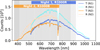 |
Fig. 1 Example stellar spectra of NGTS-5 (T; darker line) and its reference star (R; lighter line), observed with the R1000R grism on Night 1 (blue) and the R1000B grism on Night 2 (orange). The vertical lines with gray-shaded regions indicate the adopted spectroscopic passbands. |
3 Light curve analysis
The white and spectroscopic light curves were modeled following the approach of Chen et al. (2018). Each light curve was assumed to consist of a transit signal superimposed with correlated systematics.
To model the transit signal, we employed the Python package batman (Kreidberg 2015), assuming a circular orbit. The transit model was parameterized by the orbital period (P), orbital inclination (i), scaled semimajor axis (a/R⋆), planet-to-star radius ratio (Rp/R⋆), mid-transit time (tc), and stellar limb-darkening coefficients (LDCs). A four-parameter nonlinear limb-darkening law was adopted, with fixed coefficients (u1, u2, u3, and u4) derived from the PHOENIX stellar atmosphere models (Husser et al. 2013) via the Python tool of Espinoza & Jordán (2015). Light curves were then computed using the efficient numerical integration scheme implemented in batman for higher-order limb-darkening models. The stellar model grid was configured to match NGTS-5’s effective temperature (Teff = 5000 K), surface gravity (log g⋆ = 4.5), and metallicity ([Fe/H] = 0.0).
The correlated systematics were modeled using Gaussian processes (GP; Rasmussen & Williams 2006; Gibson et al. 2012), implemented via the Python package george (Ambikasaran et al. 2015). The GP mean function was defined as the product of the transit model and a polynomial trend in time, i.e.,  . The GP covariance function was specified by a 3/2-order Matérn kernel, incorporating multiple state vectors as input variables:
 (1)
(1)
where σk is the covariance amplitude, α denotes the index of individual GP input variables, and rα = |xα,i − xα,j|/τα represents the distance between the i-th and j-th inputs along the α-th dimension, normalized by its characteristic length scale τα for each input variable. The 1D 3/2-order Matérn kernel is given by
 (2)
(2)
Prior to modeling, each state vector was standardized to zero mean and unit variance. To account for potential underestimation of photometric uncertainties, an additional white noise variance term  was added to the diagonal of the covariance matrix. The GP regression thus included the free parameters σk, τα, and σw. Finally, the posterior distributions of the model parameters were explored using the affine-invariant Markov chain Monte Carlo (MCMC) algorithm, implemented with the Python package emcee (Foreman-Mackey et al. 2013).
3.1 White light curves
The white light curves from both nights were jointly fit with common transit parameters (except for the mid-transit time tc), while separate quadratic trend and GP parameters accounted for night-specific systematics. For both transits, all five state vectors {t, x, y, sy, and θ} were selected as input variables for the GP covariance matrix. This resulted in a total of 25 free parameters in the joint light curve fitting.
The orbital period was fixed to P = 3.3569866 days, as reported by Eigmüller et al. (2019), and the LDCs were fixed to their precomputed values. Uniform priors were adopted for the remaining transit parameters {i, a/R⋆, Rp/R⋆, and tc}, trend coefficients {c0, c1, and c2}, and σw, while log-uniform priors were assigned to the other GP hyper-parameters {σk, τt, τx, τy,  , and τθ}. Three chains with 60 walkers each were initialized in the MCMC process, with two short 1000-step burn-in phases followed by a production run of 5000 steps. Convergence was verified by ensuring the chain length significantly exceeded 50 times the integrated autocorrelation time.
Figure 2 shows the observed white light curves, along with the best-fit transit models and systematics. The root mean square error (RMSE) of the residuals is 386 ppm for Night 1 and 321 ppm for Night 2, corresponding to 2.8 and 2.1 times the photon noise limit, respectively. The adopted priors and resulting posteriors for the free parameters are summarized in Table 2. Our joint fit yields transit parameters of  and
and  , which deviate from the values reported in the discovery paper (i = 86.6 ± 0.2◦,
  ; Eigmüller et al. 2019) at the 3.6σ and 3.4σ levels, respectively. This discrepancy is likely attributable to the well-known degeneracy between i and a/R⋆ in transit light curve modeling, where a higher inclination correlates positively with a larger-scaled semimajor axis.
3.2 Spectroscopic light curves
Prior to modeling the spectroscopic light curves, we removed wavelength-independent systematics, known as common-mode systematics, to reduce the overall noise level (Gibson et al. 2013a,b, 2017; Stevenson et al. 2014; Chen et al. 2017b,a). For each transit, the common-mode systematics were derived by dividing the raw white light curve by its best-fit transit model. The resulting common-mode trend was then used to normalize each individual spectroscopic light curve for both nights.
After correcting for common-mode systematics, the spectroscopic light curves were individually fit for each night. For a given transit, each spectroscopic channel was modeled independently, with wavelength-dependent transit parameters and systematics parameters. The LDCs were fixed to the precomputed values. The other transit parameters {i, a/R⋆, and tc} were fixed to the median values derived from the joint white light curves analysis (Table 2). Two coefficients {c0 and c1} were used to describe a linear time trend in the GP mean function, and three state vectors {t, y, and sy} were selected as inputs to the GP covariance matrix, resulting in eight free parameters for each spectroscopic light curve. Three chains with 32 walkers each were initialized in the MCMC process, with two short 1000-step burn-in phases followed by a 5000-step production run.
Figure 3 shows the matrix of spectroscopic light curves, along with the best-fit light curve systematics models and corresponding residuals. The derived transmission spectra, along with the fixed LDCs for each spectroscopic passband, are presented in Table A.1. Figure 4 shows the individual transmission spectra for the two nights. The two spectra exhibit noticeable differences, with a chi-squared value of χ2 = 103.03 for dof = 49 in the common passbands. In the next section, we investigate the possible role of stellar activity in explaining these differences.
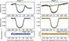 |
Fig. 2 White light curves of NGTS-5 observed with GTC/OSIRIS on Night 1 (left) and Night 2 (right). Top panels: Observed white light curves (blue circles for Night 1, orange circles for Night 2), best-fit models (black lines), and modeled systematics (green lines). Middle panels: De-trended white light curves with the best-fit transit models. Bottom panels: Residuals between the observed data and best-fit models. |
4 Atmospheric retrieval analysis
4.1 Model setup
4.1.1 Atmospheric forward model
To characterize the atmospheric properties of NGTS-5b, we performed a series of Bayesian spectral retrieval analyses on its transmission spectra. The 1D forward models were generated using the Python package petitRADTRANS 2.6.7 (Mollière et al. 2019). Bayesian parameter estimation and model comparison were conducted with the multimodal nested sampling algorithm implemented in PyMultiNest (Buchner et al. 2014), providing posterior distributions of model parameters and Bayesian evidences (𝒵).
The atmospheric temperature profile was assumed to be isothermal, with a temperature of Tiso. The pressure range from 102 to 10−6 bar was equally divided into 100 layers on a logarithmic scale. The reference pressure P0, corresponding to the planetary radius (Rp = 1.136 RJup), was treated as a free parameter to anchor the vertical structure.
Key opacity sources included gas absorption, collision-induced absorption (CIA), Rayleigh scattering, and parameterized cloud and haze contributions. The atmospheric bulk composition was assumed to be dominated by H2 and He with a 3 : 1 mass ratio, consistent with a roughly primordial composition (Mollière et al. 2019). Opacity contributions from 15 molecular and atomic species (Na, K, TiO, VO, H2O, CH4, CO, CO2, HCN, C2H2, PH3, NH3, H2S, SiO, and FeH) were included. Continuum opacity sources included CIA from H2–H2 and H2–He pairs, and Rayleigh scattering by H2 and He.
Two different approaches were employed for handling gas abundances:
Equilibrium chemistry: where the mass fractions were interpolated from precomputed chemical grids (Mollière et al. 2019), parameterized by the atmospheric metallicity (logZ) and carbon-to-oxygen number ratio (C/O).
Free chemistry: where the mass fractions (Xi) of the 15 individual opacity species were treated as independent free parameters.
Following the prescription of MacDonald & Madhusudhan (2017), clouds were modeled as a fractional coverage (ϕ) of the terminator region. The cloudy region was modeled as an opaque cloud deck parameterized by its cloud-top pressure (Pcloud), with an additional Rayleigh-like scattering component – characterized by an amplitude factor (ARS) – that enhances short-wavelength opacity. Additionally, a free vertical offset (∆offset) was introduced between the two transits to correct for potential systematic differences.
4.1.2 Stellar contamination model
We further accounted for potential contamination from stellar surface heterogeneities – specifically spots and faculae – in the retrieval analyses. These introduce wavelength-dependent variations in the observed transmission spectra due to the temperature contrast between regions in and out of the transit chord. The transit chord was simply assumed to be quiescent, as potential signatures of spot or facula crossings could not be distinguished given the level of systematics in the light curves. A wavelength-dependent correction factor, βλ, was introduced:
 (3)
(3)
where Dλ and Dλ,c are the modeled transit depths without and with stellar contamination, respectively.
The correction factor βλ depends on the relative flux contributions from the photosphere, spots, and faculae, with temperatures of Tphot, Tspot, and Tfacu at coverage fractions of 1 − fspot − ffacu, fspot, and ffacu:
![Mathematical equation: ${\beta _\lambda } = S\left( {\lambda ,{T_{{\rm{phot}}}}} \right)/\left[ {{f_{{\rm{spot}}}}S\left( {\lambda ,{T_{{\rm{spot}}}}} \right)\, + {f_{{\rm{facu}}}}S\left( {\lambda ,{T_{{\rm{facu}}}}} \right) + \left( {1 - {f_{{\rm{spot}}}} - {f_{{\rm{facu}}}}} \right)S\left( {\lambda ,{T_{{\rm{phot}}}}} \right)} \right],$](/articles/aa/full_html/2026/03/aa58041-25/aa58041-25-eq39.png) (4)
(4)
where S (λ, T) denotes the stellar spectrum interpolated from the PHOENIX spectral library (Husser et al. 2013).
To comprehensively assess the scenarios of planetary atmosphere and stellar contamination, we performed retrieval analyses under the following model assumptions:
A. Null model: no atmosphere and no stellar contamination, i.e., a flat-line model.
B. Pure atmospheric model with equilibrium chemistry.
C. Pure atmospheric model with free chemistry.
D. Pure stellar contamination model.
E. Hybrid model: equilibrium chemistry atmosphere with stellar contamination.
F. Hybrid model: free chemistry atmosphere with stellar contamination.
For model assumptions E and F, atmospheric properties remained the same for both transits while stellar contamination parameters (∆Tspot = Tspot − Tphot, ∆Tfacu = Tfacu − Tphot, fspot, and ffacu) were retrieved independently for each transit, considering the ~1-year gap between the two observations. Each retrieval run used 250 live points in PyMultiNest, typically yielding an uncertainty of ∼0.2 in ln 𝒵. For model comparison, the Bayes factor ℬ10 (ln ℬ10 = ln 𝒵1 − ln 𝒵0 = ∆ ln 𝒵10) was interpreted following the criteria of Trotta (2008): strong evidence for model 1 over model 0 if ∆ ln 𝒵10 ≥ 5.0, moderate if 2.5 ≤ ∆ ln 𝒵10 < 5.0, weak if 1.0 ≤ ∆ ln 𝒵10 < 2.5, and inconclusive if ∆ ln 𝒵10 < 1.0.
Priors and derived posteriors for the parameters used in the white light curve analyses.
4.2 Retrieval results
4.2.1 Evidence for stellar contamination
Assuming an atmospheric scale height of H/R⋆ = (1.52 ± 0.25) × 10−3, the transmission spectrum from Night 1 (522–922 nm) spans ∼9 scale heights, while that from Night 2 (366–772 nm) spans ∼5. Using the retrieval framework described above, we investigated the contributions of planetary atmosphere and stellar contamination in the transmission spectra of NGTS-5b. Summary statistics and retrieved parameters for all models are listed in Tables 3 and 4. In Table 3, detection significance (DS) is expressed in terms of the frequentist “sigma” significance level. Following Benneke & Seager (2013), the Bayes factor ℬ10 can be related to the frequentist p-value ρ via  , where e is the exponential of one and ρ is the p-value. The p-value is then converted to the corresponding sigma significance
  , where erf is the error function. This conversion is valid for ρ < e−1 (i.e., |∆ ln 𝒵| ≥ 1.0). For models with |∆ ln 𝒵| < 1.0, the corresponding significance is not reported and is labeled as N/A (not applicable).
We first assessed pure atmospheric models. While both equilibrium chemistry (Model B) and free chemistry (Model C) improve the fit relative to a flat spectrum (Model A), neither can account for the discrepancy between the two nights in the common wavelength range. We therefore introduced epoch-dependent stellar contamination in the model assumptions. Bayesian model comparison indicates that hybrid models incorporating only unocculted spots are preferred. The model with spots alone (Model D.ii) is moderately favored over the model including both spots and faculae (Model D.i; ∆ ln 𝒵 = 4.45), while the latter is decisively favored over the faculae-only model (Model D.iii; ∆ ln 𝒵 = 10.32).
Compared to pure atmospheric models, hybrid models combining atmospheric features with unocculted spot contamination yield significantly improved fits and higher Bayesian evidences, with ∆ ln 𝒵 = 16.38 for the equilibrium chemistry case (Model E.i) and ∆ ln 𝒵 = 15.75 for free chemistry (Model F.i). The corresponding retrieved transmission spectra are shown in Fig. 5. In contrast, omitting the atmospheric component (Model D) substantially decreases the Bayesian evidence (∆ ln 𝒵 > 22). This provides decisive evidence that both atmospheric signatures and stellar contamination are essential to explain the observed wavelength-dependent transit depth variations. Incorporating spot contamination also substantially reduces the night-to-night discrepancy, improving the χ2 from 103.03 to 73.18 after correcting for stellar contamination and applying a vertical offset (model F; with d.o.f. = 49).
The retrievals suggest enhanced stellar activity during Night 1, characterized by a larger spot-to-photosphere temperature contrast (−1196 to −839 K) and higher spot coverage fraction (20–29%) compared to Night 2, where the inferred contrast and coverage range from −590 to −58 K and 4–23%, respectively. This behavior reflects the known degeneracy between ∆Tspot and fspot, as illustrated in Fig. 6. These results demonstrate that stellar contamination significantly affects the transmission spectra of NGTS-5b and can lead to biased inferences of planetary properties if not properly accounted for.
Although no photometric signs of activity were found (Eigmüller et al. 2019), the Ca II H&K lines indicate that NGTS-5 is active (log  ; Vissapragada et al. 2022). Given the lack of contemporaneous photometric monitoring with our OSIRIS observations, such epoch-to-epoch variations cannot be ruled out. Active regions on K-type stars can evolve on timescales of days to weeks, typically modulated by stellar rotation (Zhang et al. 2020). Similar epoch-to-epoch variations in stellar contamination have been reported for other warm Saturn- and sub-Saturn-mass planets orbiting K-type stars, such as HAT-P-12b (Jiang et al. 2021), HAT-P-18b (Fournier-Tondreau et al. 2024; Perdelwitz et al. 2025), and WASP-69b (Petit dit de la Roche et al. 2024). Discrepancies where photometric monitoring suggests lower activity levels than transmission spectroscopy are not uncommon in the literature (e.g., for WASP-69b; Murgas et al. 2020; Estrela et al. 2021; Ouyang et al. 2023; Petit dit de la Roche et al. 2024; Chakraborty et al. 2024). However, while these epoch-to-epoch variations remain physically plausible, we caution that the activity inferred using the disk-integrated prescription of the TLS effect (Rackham et al. 2018, 2019) might be overestimated due to degeneracies and model oversimplification (Sumida et al. 2026).
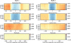 |
Fig. 3 Spectroscopic light curves of NGTS-5 observed with GTC/OSIRIS on Night 1 (left) and Night 2 (right). First row: matrix of the raw light curves. Second row: matrix of the de-trended light curves. Third row: Matrix of the extracted systematics. Fourth row: matrix of the residuals. |
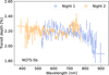 |
Fig. 4 Individual transmission spectra of NGTS-5b derived from Night 1 (blue) and Night 2 (orange) observations. |
Summary of Bayesian spectral retrieval statistics.
4.2.2 Constraints on the planetary atmosphere properties
The atmospheric properties retrieved from the two hybrid models are broadly consistent with each other, with discrepancies within 1.5σ for key parameters including atmospheric temperature, reference pressure, cloud-top pressure, and haze enhancement factor.
The hybrid model assuming equilibrium chemistry yields well-constrained posteriors for the atmospheric temperature ( ), reference pressure (log
  log bar), and haze enhancement factor (log
  ). The retrieved cloud-top pressure and cloud fraction posterior distributions are skewed toward the upper boundary of the prior (log Pcloud > 0.81 log bar, ϕ > 0.56, at the 90% lower limit), suggesting a relatively clear atmosphere with nearly uniform low-altitude cloud coverage. Additionally, the retrieval results indicate a low atmospheric metallicity of
  times solar and a C/O ratio skewed to the lower boundary of the prior (C/O < 0.22, 90% upper limit).
The hybrid model with free chemistry produces atmospheric parameters consistent with the equilibrium chemistry case. Specifically, it retrieves  , log P0 < −4.75 log bar (90% upper limit),
  log bar, and
  . The cloud fraction posterior is skewed toward the lower prior bound (ϕ < 0.45, 90% upper limit), also indicating a relatively clear atmosphere. Among the 15 chemical species considered in the free chemistry model, only the mass fractions of K, H2O, and FeH are constrained, with retrieved values of
  ,
,  , and
, and  , respectively.
To assess the individual contributions of these species, we performed a set of retrievals by sequentially removing each of the 15 species from the free chemistry model and comparing the resulting Bayesian evidence. As summarized in Table 3, this analysis provides strong evidence for the presence of H2O (∆ ln 𝒵 = 5.91), while the evidence for K (∆ ln 𝒵 = −0.02) and FeH (∆ ln 𝒵 = 0.49) remains inconclusive.
Finally, to quantify the impact of stellar contamination on atmospheric retrieval, we compared the posterior distributions of the atmospheric parameters from models with and without stellar contamination (Fig. 7). The inclusion of stellar contamination leads to more tightly constrained and systematically higher retrieved mass fractions of H2O, K, and FeH. This underscores the importance of properly accounting for stellar contamination. Neglecting such effects can suppress spectral features and bias atmospheric inferences.
5 Discussion
Our retrieval analyses of the transmission spectra suggest that NGTS-5b possesses a relatively clear atmosphere dominated by water absorption, regardless of whether equilibrium or free chemistry is assumed. Given its equilibrium temperature of 952 ± 24 K and mass of 0.229 ± 0.037 MJup (Eigmüller et al. 2019), this result is consistent with NGTS-5b’s proximity to the so-called “clear sky corridor” (Ashtari et al. 2025) spanning 700–1700 K, where the 1.4 µm H2O absorption band is typically stronger.
Under the equilibrium chemistry assumption, our retrieval yields subsolar values for both atmospheric metallicity ( ) and C/O (
 ). These values may be biased due to the limited wavelength coverage of GTC/OSIRIS in the optical, where H2O bands are relatively weaker than in the infrared, and where the absence of detectable carbon-bearing species limits the constraints on carbon abundance. Assuming the host star’s metallicity of 0.12 ± 0.1 dex, we find that NGTS-5b’s mass and atmospheric metallicity are broadly consistent with the mass-metallicity relation established from exoplanet transmission spectra (Welbanks et al. 2019; Sun et al. 2024). The deviation from the predicted bulk metallicity could indicate a locally well-mixed interior status (Thorngren et al. 2016; Mordasini et al. 2016; Hasegawa & Swain 2024; Swain et al. 2024).
The free chemistry retrieval yields a mass fraction of  . This corresponds to a log volume mixing ratio (log VMR) of
  , comparable to values frequently retrieved in recent JWST studies, such as those for WASP-80b (
 ; Bell et al. 2023), WASP-94b (
 ; Ahrer et al. 2025), WASP-107b (
 ; Sing et al. 2024), and HAT-P-12b (
 ; Crouzet et al. 2025). While HAT-P-12b (0.21 MJup, 963 K, K4 host; Hartman et al. 2009) represents a very similar system in terms of both planetary mass and equilibrium temperature, another comparable planet, HAT-P-18b (0.20 MJup, 852 K, K2 host; Hartman et al. 2011), exhibits a much lower H2O abundance (
 ; Fournier-Tondreau et al. 2024), hinting at potential atmospheric diversity among these warm Saturns.
From the free chemistry retrieval, we derived a mean molecular weight of  . This indicates an H2-dominated atmosphere and corresponds to a metallicity range of 3–50× solar under the assumption of chemical equilibrium, regardless of the adopted C/O ratio. This apparent inconsistency with the subsolar metallicity derived from the equilibrium chemistry retrieval likely results from the limited spectral coverage and precision of current measurements, which restrict the ability to jointly constrain several key molecular species. Resolving this discrepancy will require additional observations to break the degeneracy between reference pressure, cloud property, metallicity, and molecular abundances. As demonstrated by the benchmark planet WASP-39b, where the retrieved values for H2O ranged from log VMR ∼ −1.13 to log VMR ∼ −6.35 depending on the JWST instrumental mode and atmospheric model, any interpretation of abundances should be approached with caution (Lueber et al. 2024).
We also note that the retrieved atmospheric temperatures of NGTS-5b under both equilibrium and free-chemistry assumptions are approximately 250–350 K lower than the corresponding equilibrium temperature. This discrepancy has been widely reported in exoplanet transmission spectroscopy. One possible explanation is that 1D retrieval models can produce biased temperature estimates when applied to atmospheres with inhomogeneous terminator properties (MacDonald et al. 2020). Recent studies show that even planets with equilibrium temperatures as low as 770 K can exhibit substantial morning-to-evening limb asymmetry (e.g., Murphy et al. 2024).
Future infrared observations with JWST, capable of detecting the major carbon-, oxygen-, sulfur-, and nitrogen-bearing species, will be critical for confirming the presence of H2O and for robustly constraining atmospheric metallicity and elemental enrichment patterns. At the same time, the frequent presence of stellar contamination, as revealed by transmission spectroscopy, highlights the importance of complementary blue-optical observations, which have their strongest impact at ultraviolet and blue-optical wavelengths where the contrast between active regions and the quiescent photosphere is most pronounced (Iyer & Line 2020; Fairman et al. 2024; Saba et al. 2025). Together, these infrared and optical observations will enable precise measurements of elemental ratios (e.g., C/O) and metallicity (or [O/H]), ultimately providing insights into NGTS-5b’s formation and migration pathways (Öberg et al. 2011; Madhusudhan et al. 2014, 2017; Penzlin et al. 2024; Ohno et al. 2025).
Priors and derived posteriors for the parameters used in the spectral retrieval analyses.
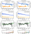 |
Fig. 5 Transmission spectra of NGTS-5b with the median, 1σ, and 2σ confidence intervals of the retrieved hybrid model assuming equilibrium chemistry (Model E, left) and free chemistry (Model F, right). Top row: transmission spectra and retrieved models incorporating both atmospheric and stellar contamination effects, after correcting for the best-fit vertical offset (∆offset) derived from the joint retrieval. Second row: wavelength-dependent stellar contamination factors inferred from the retrieval. Third row: transmission spectra and corresponding models after correcting for stellar contamination. Bottom row: Reference models illustrating the individual contributions of key species. |
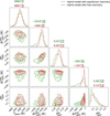 |
Fig. 6 Posterior distributions of the stellar contamination parameters for the retrieved hybrid model assuming equilibrium chemistry (Model E) and free chemistry (Model F). Diagonal panels: marginalized distributions for each parameter. Detailed posterior values are listed in Table 4. |
6 Conclusions
As a warm sub-Saturn just above the upper boundary of the short-period Neptunian desert (Mazeh et al. 2016) – potentially shaped by tidal disruption following high-eccentricity migration (Matsakos & Königl 2016; Owen & Lai 2018) – NGTS-5b offers valuable opportunities to probe the formation and evolutionary history of close-in low-mass giant planets. In this work, we presented optical transmission spectra of NGTS-5b obtained from two transits observed with GTC/OSIRIS. Our analyses identified systematic discrepancies between the two observed spectra, which we attribute to varying levels of unocculted stellar activity across the two epochs.
By incorporating epoch-dependent stellar contamination alongside planetary atmospheric models in a joint retrieval framework, we found decisive Bayesian evidence (∆ ln 𝒵 > 15) for the presence of stellar contamination, independent of atmospheric assumptions. The retrieved stellar activity parameters indicate enhanced activity during the first night, characterized by a larger spot-to-photosphere temperature contrast and higher spot coverage fraction relative to the second night. The discrepancies between the two transmission spectra were substantially reduced after correcting for these stellar contamination effects.
Atmospheric retrievals assuming both equilibrium and free chemistry consistently indicate a relatively clear atmosphere for NGTS-5b, with water vapor identified as the dominant opacity source. However, the retrieved atmospheric metallicities differ between assumptions, being subsolar under equilibrium chemistry and supersolar in the free chemistry case. We attribute this inconsistency to the limited wavelength coverage of GTC/OSIRIS, which includes only weak water bands and lacks diagnostic features from other key oxygen- and carbon-bearing species.
To robustly constrain the atmospheric composition and elemental ratios of NGTS-5b, future observations spanning a broader wavelength range, particularly in the infrared with JWST, complemented by blue-optical measurements with HST and large ground-based facilities, will be essential. Such comprehensive spectroscopic coverage will not only improve constraints on atmospheric metallicity and C/O ratio but also help mitigate the effects of stellar contamination, enabling a more complete understanding of the formation, migration, and evolutionary processes shaping this warm sub-Saturn.
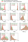 |
Fig. 7 Posterior distributions of the retrieved planetary atmosphere properties assuming free chemistry, comparing results with (red) and without (green) stellar contamination. The dashed lines mark the median values and the corresponding 1σ credible intervals. Unconstrained parameters are not shown. |
Data availability
The reduced light curves presented in this work are available at the CDS via https://cdsarc.cds.unistra.fr/viz-bin/cat/J/A+A/707/A315
Acknowledgements
We thank the anonymous referees for their constructive comments and suggestions. G.C. acknowledges the support by the National Natural Science Foundation of China (NSFC grant Nos. 42578016, 12122308, 42075122), Youth Innovation Promotion Association CAS (2021315), and the Minor Planet Foundation of the Purple Mountain Observatory. This work is based on observations made with the Gran Telescopio Canarias installed at the Spanish Observatorio del Roque de los Muchachos of the Instituto de Astrofísica de Canarias on the island of La Palma.
References
- Ahrer, E.-M., Gandhi, S., Alderson, L., et al. 2025, MNRAS, 540, 2535 [Google Scholar]
- Ambikasaran, S., Foreman-Mackey, D., Greengard, L., Hogg, D. W., & O’Neil, M. 2015, IEEE Trans. Pattern Anal. Mach. Intell., 38, 252 [Google Scholar]
- Apai, D., Rackham, B. V., Giampapa, M. S., et al. 2018, arXiv e-prints [arXiv:1803.08708] [Google Scholar]
- Ashtari, R., Stevenson, K. B., Sing, D., et al. 2025, AJ, 169, 106 [Google Scholar]
- Baluev, R. V., Sokov, E. N., Sokova, I. A., et al. 2021, Acta Astron., 71, 25 [NASA ADS] [Google Scholar]
- Banerjee, A., Barstow, J. K., Gressier, A., et al. 2024, ApJ, 975, L11 [Google Scholar]
- Barros, S. C. C., Boué, G., Gibson, N. P., et al. 2013, MNRAS, 430, 3032 [NASA ADS] [CrossRef] [Google Scholar]
- Bell, T. J., Welbanks, L., Schlawin, E., et al. 2023, Nature, 623, 709 [Google Scholar]
- Benneke, B., & Seager, S. 2013, ApJ, 778, 153 [Google Scholar]
- Buchner, J., Georgakakis, A., Nandra, K., et al. 2014, A&A, 564, A125 [NASA ADS] [CrossRef] [EDP Sciences] [Google Scholar]
- Cepa, J., Aguiar, M., Escalera, V. G., et al. 2000, SPIE Conf. Ser., 4008, 623 [Google Scholar]
- Chakraborty, H., Lendl, M., Akinsanmi, B., Petit dit de la Roche, D. J. M., & Deline, A. 2024, A&A, 685, A173 [NASA ADS] [CrossRef] [EDP Sciences] [Google Scholar]
- Chen, G., Guenther, E. W., Pallé, E., et al. 2017a, A&A, 600, A138 [NASA ADS] [CrossRef] [EDP Sciences] [Google Scholar]
- Chen, G., Pallé, E., Nortmann, L., et al. 2017b, A&A, 600, L11 [NASA ADS] [CrossRef] [EDP Sciences] [Google Scholar]
- Chen, G., Pallé, E., Welbanks, L., et al. 2018, A&A, 616, A145 [NASA ADS] [CrossRef] [EDP Sciences] [Google Scholar]
- Chen, G., Casasayas-Barris, N., Pallé, E., et al. 2020, A&A, 642, A54 [NASA ADS] [CrossRef] [EDP Sciences] [Google Scholar]
- Chen, G., Pallé, E., Parviainen, H., Murgas, F., & Yan, F. 2021, ApJ, 913, L16 [NASA ADS] [CrossRef] [Google Scholar]
- Crouzet, N., Edwards, B., Konings, T., et al. 2025, A&A, 703, A264 [NASA ADS] [CrossRef] [EDP Sciences] [Google Scholar]
- Dyrek, A., Min, M., Decin, L., et al. 2024, Nature, 625, 51 [Google Scholar]
- Eastman, J., Siverd, R., & Gaudi, B. S. 2010, PASP, 122, 935 [Google Scholar]
- Eigmüller, P., Chaushev, A., Gillen, E., et al. 2019, A&A, 625, A142 [NASA ADS] [CrossRef] [EDP Sciences] [Google Scholar]
- Espinoza, N., & Jordán, A. 2015, MNRAS, 450, 1879 [Google Scholar]
- Estrela, R., Swain, M. R., Roudier, G. M., et al. 2021, AJ, 162, 91 [NASA ADS] [CrossRef] [Google Scholar]
- Fairman, C., Wakeford, H. R., & MacDonald, R. J. 2024, AJ, 167, 240 [Google Scholar]
- Foreman-Mackey, D., Hogg, D. W., Lang, D., & Goodman, J. 2013, PASP, 125, 306 [Google Scholar]
- Fournier-Tondreau, M., MacDonald, R. J., Radica, M., et al. 2024, MNRAS, 528, 3354 [NASA ADS] [CrossRef] [Google Scholar]
- Gibson, N. P., Aigrain, S., Roberts, S., et al. 2012, MNRAS, 419, 2683 [NASA ADS] [CrossRef] [Google Scholar]
- Gibson, N. P., Aigrain, S., Barstow, J. K., et al. 2013a, MNRAS, 428, 3680 [Google Scholar]
- Gibson, N. P., Aigrain, S., Barstow, J. K., et al. 2013b, MNRAS, 436, 2974 [CrossRef] [Google Scholar]
- Gibson, N. P., Nikolov, N., Sing, D. K., et al. 2017, MNRAS, 467, 4591 [NASA ADS] [CrossRef] [Google Scholar]
- Hartman, J. D., Bakos, G. Á., Torres, G., et al. 2009, ApJ, 706, 785 [NASA ADS] [CrossRef] [Google Scholar]
- Hartman, J. D., Bakos, G. Á., Sato, B., et al. 2011, ApJ, 726, 52 [NASA ADS] [CrossRef] [Google Scholar]
- Hasegawa, Y., & Swain, M. R. 2024, ApJ, 973, L46 Horne, K. 1986, PASP, 98, 609 [Google Scholar]
- Husser, T.-O., Wende-von Berg, S., Dreizler, S., et al. 2013, A&A, 553, A6 [NASA ADS] [CrossRef] [EDP Sciences] [Google Scholar]
- Iyer, A. R., & Line, M. R. 2020, ApJ, 889, 78 [Google Scholar]
- Jiang, C., Chen, G., Pallé, E., et al. 2021, A&A, 656, A114 [NASA ADS] [CrossRef] [EDP Sciences] [Google Scholar]
- Jiang, C., Chen, G., Pallé, E., et al. 2023, A&A, 675, A62 [NASA ADS] [CrossRef] [EDP Sciences] [Google Scholar]
- Jiang, C., Chen, G., Murgas, F., et al. 2024, A&A, 682, A73 [NASA ADS] [CrossRef] [EDP Sciences] [Google Scholar]
- Kang, H., Chen, G., Jiang, C., et al. 2024, A&A, 687, A9 [NASA ADS] [CrossRef] [EDP Sciences] [Google Scholar]
- Kirk, J., Wheatley, P. J., Louden, T., et al. 2016, MNRAS, 463, 2922 [NASA ADS] [CrossRef] [Google Scholar]
- Kirk, J., Ahrer, E.-M., Claringbold, A. B., et al. 2025, MNRAS, 537, 3027 [Google Scholar]
- Kreidberg, L. 2015, PASP, 127, 1161 [Google Scholar]
- Libby-Roberts, J. E., Schutte, M., Hebb, L., et al. 2023, AJ, 165, 249 [NASA ADS] [CrossRef] [Google Scholar]
- Lim, O., Benneke, B., Doyon, R., et al. 2023, ApJ, 955, L22 [NASA ADS] [CrossRef] [Google Scholar]
- Lueber, A., Novais, A., Fisher, C., & Heng, K. 2024, A&A, 687, A110 [NASA ADS] [CrossRef] [EDP Sciences] [Google Scholar]
- MacDonald, R. J., & Madhusudhan, N. 2017, MNRAS, 469, 1979 [Google Scholar]
- MacDonald, R. J., Goyal, J. M., & Lewis, N. K. 2020, ApJ, 893, L43 [NASA ADS] [CrossRef] [Google Scholar]
- Madhusudhan, N. 2019, ARA&A, 57, 617 [Google Scholar]
- Madhusudhan, N., Amin, M. A., & Kennedy, G. M. 2014, ApJ, 794, L12 [Google Scholar]
- Madhusudhan, N., Bitsch, B., Johansen, A., & Eriksson, L. 2017, MNRAS, 469, 4102 [NASA ADS] [CrossRef] [Google Scholar]
- Matsakos, T., & Königl, A. 2016, ApJ, 820, L8 [Google Scholar]
- Mazeh, T., Holczer, T., & Faigler, S. 2016, A&A, 589, A75 [NASA ADS] [CrossRef] [EDP Sciences] [Google Scholar]
- Mohler-Fischer, M., Mancini, L., Hartman, J. D., et al. 2013, A&A, 558, A55 [NASA ADS] [CrossRef] [EDP Sciences] [Google Scholar]
- Mollière, P., Wardenier, J. P., van Boekel, R., et al. 2019, A&A, 627, A67 [Google Scholar]
- Moran, S. E., Stevenson, K. B., Sing, D. K., et al. 2023, ApJ, 948, L11 [NASA ADS] [CrossRef] [Google Scholar]
- Mordasini, C., van Boekel, R., Mollière, P., Henning, T., & Benneke, B. 2016, ApJ, 832, 41 [Google Scholar]
- Murgas, F., Chen, G., Pallé, E., Nortmann, L., & Nowak, G. 2019, A&A, 622, A172 [NASA ADS] [CrossRef] [EDP Sciences] [Google Scholar]
- Murgas, F., Chen, G., Nortmann, L., Palle, E., & Nowak, G. 2020, A&A, 641, A158 [NASA ADS] [CrossRef] [EDP Sciences] [Google Scholar]
- Murphy, M. M., Beatty, T. G., Schlawin, E., et al. 2024, Nat. Astron., 8, 1562 [NASA ADS] [CrossRef] [Google Scholar]
- Nikolov, N., Sing, D. K., Fortney, J. J., et al. 2018, Nature, 557, 526 [CrossRef] [Google Scholar]
- Öberg, K. I., Murray-Clay, R., & Bergin, E. A. 2011, ApJ, 743, L16 [Google Scholar]
- Ohno, K., Ikoma, M., Okuzumi, S., & Kimura, T. 2025, PASJ, accepted [arXiv:2506.16060] [Google Scholar]
- Ouyang, Q., Wang, W., Zhai, M., et al. 2023, MNRAS, 521, 5860 [NASA ADS] [CrossRef] [Google Scholar]
- Owen, J. E., & Lai, D. 2018, MNRAS, 479, 5012 [Google Scholar]
- Parviainen, H., Pallé, E., Chen, G., et al. 2018, A&A, 609, A33 [NASA ADS] [CrossRef] [EDP Sciences] [Google Scholar]
- Penzlin, A. B. T., Booth, R. A., Kirk, J., et al. 2024, MNRAS, 535, 171 [NASA ADS] [CrossRef] [Google Scholar]
- Perdelwitz, V., Chaikin-Lifshitz, A., Ofir, A., & Aharonson, O. 2025, ApJ, 980, L42 [Google Scholar]
- Petit dit de la Roche, D. J. M., Chakraborty, H., Lendl, M., et al. 2024, A&A, 692, A83 [NASA ADS] [CrossRef] [EDP Sciences] [Google Scholar]
- Powell, D., Feinstein, A. D., Lee, E. K. H., et al. 2024, Nature, 626, 979 [NASA ADS] [CrossRef] [Google Scholar]
- Rackham, B., Espinoza, N., Apai, D., et al. 2017, ApJ, 834, 151 [Google Scholar]
- Rackham, B. V., Apai, D., & Giampapa, M. S. 2018, ApJ, 853, 122 [Google Scholar]
- Rackham, B. V., Apai, D., & Giampapa, M. S. 2019, AJ, 157, 96 [Google Scholar]
- Radica, M., Welbanks, L., Espinoza, N., et al. 2023, MNRAS, 524, 835 [NASA ADS] [CrossRef] [Google Scholar]
- Rasmussen, C. E., & Williams, C. K. I. 2006, Gaussian Processes for Machine Learning [Google Scholar]
- Rustamkulov, Z., Sing, D. K., Mukherjee, S., et al. 2023, Nature, 614, 659 [NASA ADS] [CrossRef] [Google Scholar]
- Saba, A., Thompson, A., Yip, K. H., et al. 2025, ApJS, 276, 70 [Google Scholar]
- Seager, S., & Sasselov, D. D. 2000, ApJ, 537, 916 [Google Scholar]
- Sing, D. K., Rustamkulov, Z., Thorngren, D. P., et al. 2024, Nature, 630, 831 [NASA ADS] [CrossRef] [Google Scholar]
- Solanki, S. K. 2003, A&A Rev., 11, 153 [Google Scholar]
- Stevenson, K. B., Bean, J. L., Seifahrt, A., et al. 2014, AJ, 147, 161 [NASA ADS] [CrossRef] [Google Scholar]
- Sumida, V. Y. D., Estrela, R., Swain, M., & Valio, A. 2026, A&A, 706, A281 [NASA ADS] [CrossRef] [EDP Sciences] [Google Scholar]
- Sun, Q., Wang, S. X., Welbanks, L., Teske, J., & Buchner, J. 2024, AJ, 167, 167 [CrossRef] [Google Scholar]
- Swain, M. R., Hasegawa, Y., Thorngren, D. P., & Roudier, G. M. 2024, Space Sci. Rev., 220, 61 [Google Scholar]
- Szabó, G. M., & Kiss, L. L. 2011, ApJ, 727, L44 [Google Scholar]
- Thorngren, D. P., Fortney, J. J., Murray-Clay, R. A., & Lopez, E. D. 2016, ApJ, 831, 64 [NASA ADS] [CrossRef] [Google Scholar]
- Tody, D. 1993, in Astronomical Society of the Pacific Conference Series, 52, Astronomical Data Analysis Software and Systems II, eds. R. J. Hanisch, R. J. V. Brissenden, & J. Barnes, 173 [NASA ADS] [Google Scholar]
- Trotta, R. 2008, Contemp. Phys., 49, 71 [Google Scholar]
- Unruh, Y. C., Solanki, S. K., & Fligge, M. 1999, A&A, 345, 635 [NASA ADS] [Google Scholar]
- Vissapragada, S., Knutson, H. A., Greklek-McKeon, M., et al. 2022, AJ, 164, 234 [NASA ADS] [CrossRef] [Google Scholar]
- Welbanks, L., Madhusudhan, N., Allard, N. F., et al. 2019, ApJ, 887, L20 [NASA ADS] [CrossRef] [Google Scholar]
- Zacharias, N., Finch, C. T., Girard, T. M., et al. 2012, VizieR Online Data Catalog: UCAC4 Catalogue (Zacharias+, 2012), VizieR On-line Data Catalog: I/322A. Originally published in: 2013AJ….145…44Z [Google Scholar]
- Zhang, J., Bi, S., Li, Y., et al. 2020, ApJS, 247, 9 [NASA ADS] [CrossRef] [Google Scholar]
Appendix A Additional tables and figures
Derived transmission spectra of NGTS-5b and the corresponding adopted LDCs for each spectroscopic channel.
All Tables
Priors and derived posteriors for the parameters used in the white light curve analyses.
Priors and derived posteriors for the parameters used in the spectral retrieval analyses.
Derived transmission spectra of NGTS-5b and the corresponding adopted LDCs for each spectroscopic channel.
All Figures
|
Fig. 1 Example stellar spectra of NGTS-5 (T; darker line) and its reference star (R; lighter line), observed with the R1000R grism on Night 1 (blue) and the R1000B grism on Night 2 (orange). The vertical lines with gray-shaded regions indicate the adopted spectroscopic passbands. |
| In the text | |
|
Fig. 2 White light curves of NGTS-5 observed with GTC/OSIRIS on Night 1 (left) and Night 2 (right). Top panels: Observed white light curves (blue circles for Night 1, orange circles for Night 2), best-fit models (black lines), and modeled systematics (green lines). Middle panels: De-trended white light curves with the best-fit transit models. Bottom panels: Residuals between the observed data and best-fit models. |
| In the text | |
|
Fig. 3 Spectroscopic light curves of NGTS-5 observed with GTC/OSIRIS on Night 1 (left) and Night 2 (right). First row: matrix of the raw light curves. Second row: matrix of the de-trended light curves. Third row: Matrix of the extracted systematics. Fourth row: matrix of the residuals. |
| In the text | |
|
Fig. 4 Individual transmission spectra of NGTS-5b derived from Night 1 (blue) and Night 2 (orange) observations. |
| In the text | |
|
Fig. 5 Transmission spectra of NGTS-5b with the median, 1σ, and 2σ confidence intervals of the retrieved hybrid model assuming equilibrium chemistry (Model E, left) and free chemistry (Model F, right). Top row: transmission spectra and retrieved models incorporating both atmospheric and stellar contamination effects, after correcting for the best-fit vertical offset (∆offset) derived from the joint retrieval. Second row: wavelength-dependent stellar contamination factors inferred from the retrieval. Third row: transmission spectra and corresponding models after correcting for stellar contamination. Bottom row: Reference models illustrating the individual contributions of key species. |
| In the text | |
|
Fig. 6 Posterior distributions of the stellar contamination parameters for the retrieved hybrid model assuming equilibrium chemistry (Model E) and free chemistry (Model F). Diagonal panels: marginalized distributions for each parameter. Detailed posterior values are listed in Table 4. |
| In the text | |
|
Fig. 7 Posterior distributions of the retrieved planetary atmosphere properties assuming free chemistry, comparing results with (red) and without (green) stellar contamination. The dashed lines mark the median values and the corresponding 1σ credible intervals. Unconstrained parameters are not shown. |
| In the text | |
Current usage metrics show cumulative count of Article Views (full-text article views including HTML views, PDF and ePub downloads, according to the available data) and Abstracts Views on Vision4Press platform.
Data correspond to usage on the plateform after 2015. The current usage metrics is available 48-96 hours after online publication and is updated daily on week days.
Initial download of the metrics may take a while.