| Issue |
A&A
Volume 707, March 2026
|
|
|---|---|---|
| Article Number | A264 | |
| Number of page(s) | 12 | |
| Section | Galactic structure, stellar clusters and populations | |
| DOI | https://doi.org/10.1051/0004-6361/202558238 | |
| Published online | 08 April 2026 | |
Astrometric microlensing probes of the isolated neutron star population with Roman
1
Zentrum für Astronomie der Universität Heidelberg, Astronomisches Rechen-Institut,
Mönchhofstr. 12-14,
69120
Heidelberg,
Germany
2
Georgia Institute of Technology,
837 State St.,
Atlanta,
GA
30309,
USA
3
Space Science Institute, Lawrence Livermore National Laboratory,
7000 East Ave.,
Livermore,
CA
94550,
USA
★ Corresponding author: This email address is being protected from spambots. You need JavaScript enabled to view it.
Received:
24
November
2025
Accepted:
9
February
2026
Abstract
Context. Notoriously hard to detect and study, isolated neutron stars (NSs) might provide valuable answers to fundamental questions about stellar evolution and explosion physics. With the upcoming Roman Space Telescope, scheduled for launch in 2026, a new and powerful channel for their detection will become available: astrometric microlensing.
Aims. We set out to create a realistic sample of simulated gravitational microlensing events as observed by Roman with the Galactic Bulge Time Domain Survey. We focus in particular on the population of NS lenses, which has until now been largely understudied.
Methods. We used dedicated Galactic models tailored for application to microlensing by compact objects. In addition to populations of stars, white dwarfs, and black holes, we simulated four different NS populations with Maxwellian natal kick distributions: v = (150, 250, 350, 450) km/s. For each simulation, we applied projected Roman precision, cadence, and detectability criteria.
Results. We found that the parameter space log10 tE–log10 θE, which will be accessible to Roman observations, is efficient for the classification of stellar remnants. We found a feature in this space that is characteristic of NSs; using this feature, optimal samples of NS candidates can be constructed from Roman-like datasets. We describe the dependence of the observable parameter distributions on the assumed mean kick velocities. As the effects of natal kicks are very complex and mutually counteracting, we suggest that more detailed studies focused on the dynamics of NSs are needed in anticipation of Roman and future surveys. We estimate that Roman will observe approximately 11 000 microlensing events, including ~100 with NS lenses, whose photometric and astrometric signals are detectable; the event yield decreases by 38% when gap-filling low-cadence observations are not included. We make all simulated microlensing event datasets publicly available in preparation for Roman data.
Key words: gravitational lensing: micro / astrometry / stars: neutron / Galaxy: bulge
© The Authors 2026
 Open Access article, published by EDP Sciences, under the terms of the Creative Commons Attribution License (https://creativecommons.org/licenses/by/4.0), which permits unrestricted use, distribution, and reproduction in any medium, provided the original work is properly cited.
This article is published in open access under the Subscribe to Open model. This email address is being protected from spambots. You need JavaScript enabled to view it. to support open access publication.
1 Introduction
Neutron stars (NSs) are among the most extreme objects in the present-day Universe (Annala et al. 2023), with core densities greatly exceeding the nuclear saturation limit (Haensel et al. 2007; Koehn et al. 2025). Since such environments cannot be reproduced on Earth, NSs are natural laboratories for studying matter in extreme pressure and density conditions (Lattimer & Prakash 2004; Haensel et al. 2007). The equation of state (EoS) describing NSs is not yet accurately known (Malik et al. 2024; Chatziioannou et al. 2025; Ji et al. 2025); its applications reach far beyond astrophysics and into fundamental physics, in particular, nuclear physics and quantum chromodynamics (e.g. Baym et al. 2018; Lattimer 2021; Kumar et al. 2024). As allowed by some EoSs, NSs are speculated to contain a phase transition to exotic phases of matter (Lattimer & Prakash 2004; Annala et al. 2020, 2023), and astrophysical observations in the near future might be decisive in confirming or rejecting this hypothesis (Somasundaram et al. 2023). Since the EoS defines physical properties of NSs, including the mass-radius relation, minimum and maximum masses, and the overall mass distribution, it is strongly connected to astrophysical observations and can be constrained by them (Lattimer 2012; Fraga et al. 2016; Baym et al. 2018; Ji et al. 2025).
One of the great unknowns regarding NSs is the mechanism through which they are born. Although it has long been known that NSs experience strong natal kicks (Gunn & Ostriker 1970; Lyne & Loimer 1994; Tauris et al. 1999; Hobbs et al. 2005), their velocity distribution is still highly uncertain, and mean kick velocities varying between 100 and 500 kms−1 are assumed (e.g. Kalogera et al. 1998; Hobbs et al. 2005; Bray & Eldridge 2016; Igoshev 2020; Igoshev et al. 2021; Fortin et al. 2022; Kapil et al. 2023; O’Doherty et al. 2023; Disberg et al. 2025). Several physical mechanisms for the origin of kicks have been proposed, resulting in distinctly different kick distributions (e.g. Lai 2004; Janka 2017; Janka & Kresse 2024). It is important for our understanding and modelling of supernovae to verify theoretical predictions for natal kicks (Podsiadlowski et al. 2005; Mandel & Müller 2020; Janka & Kresse 2024). Population synthesis codes are reliant on natal kick prescriptions, which affect their predictions of gravitational wave observables (Giacobbo & Mapelli 2020) and interpretations of the nature of the observed sources (Zevin et al. 2020).
The mass distribution of NSs is also unknown, and the putative mass gap observed between high-mass NSs and low-mass black holes (BHs; Bailyn et al. 1998; Özel et al. 2010; Farr et al. 2011; Shao 2022; El-Badry et al. 2024) presents an open problem. It is unclear whether this mass gap is caused by an astrophysical mechanism (e.g. Belczynski et al. 2012) or observational biases (e.g. Wyrzykowski & Mandel 2020). While numerous isolated NSs have been found through their pulsar emission (Hewish et al. 1968; Bell Burnell 2017), NS masses can only be measured if they are in binaries, whether via observations of gravitational wave mergers (Abbott et al. 2017, 2020, 2021), X-ray binaries (e.g. Bhattacharyya 2010; Rawls et al. 2011; Kim et al. 2021), pulsar timing (e.g. Taylor et al. 1979; Reardon et al. 2016), or astrometric wobble of the companion (El-Badry et al. 2024)1. These NSs only represent rigidly defined evolutionary tracks and may not constitute a fully representative sample (e.g. El-Badry et al. 2024 expect their NS sample to have originated in primordial binaries that survived the supernova explosions, and to have undergone very weak kicks). NS masses and kicks are correlated and both depend on the progenitor mass (Stone 1982; Mandel & Müller 2020); kicks are also dependent on binarity (Podsiadlowski et al. 2005). Furthermore, being part of a binary system can also change the NS parameters through mass transfer: the fastest-rotating and most massive known pulsar is a striking example of this effect (Fonseca et al. 2021; Romani et al. 2022). In summary, the sample of NSs with measured masses is subject to complex selection effects.
This complicated interplay between evolutionary tracks and physical parameters of compact objects could be made clearer with the help of gravitational microlensing. This powerful technique of studying our Galaxy can be used to discover inherently dark objects, including compact objects (Paczynski 1996). As microlensing requires a very close chance alignment of a light-deflecting mass and a luminous source, it is very rare; continuous monitoring of millions of stars, typically in the densest regions of the sky, is needed to secure detections (e.g. Paczynski 1991). Hence, the potential of this technique has been realised on a large scale with specialised variability surveys (e.g. Udalski et al. 2015; Sumi et al. 2013; Kim et al. 2016), which today publish databases of ~10 000 microlensing events (at a rate of thousands of events per year, e.g. Mróz et al. 2020; Husseiniova et al. 2021; Shin et al. 2024), including events caused by stellar remnants. Microlensing has recently yielded the first confirmed discovery of an isolated stellar origin BH, OB110462 (Sahu et al. 2022; Lam et al. 2022a; Mróz et al. 2022), setting the track for future population studies (Lam et al. 2023; Perkins et al. 2024). A recent analysis of a white dwarf (WD) by McGill et al. (2023) showed how a microlensing mass measurement can verify theoretical predictions for the compact object structure and composition.
As of today, NSs still evade high-confidence microlensing detections. Despite extensive searches, no upcoming alignments of known pulsars with background stars close enough to cause a measurable microlensing signal have been found because the pulsar sample is simply too small (Schwarz & Seidel 2002; Ofek 2018; Harding et al. 2018; Lu & Xie 2024). On the other hand, while numerous previously unknown dark lenses are found in variability surveys, insufficient constraints on mass prevent their confident classification as NSs. Within bounds allowed by the available data, the NS candidate events might also be explained by a WD, a BH, or stellar lenses (e.g. Wyrzykowski et al. 2016; Wyrzykowski & Mandel 2020; Lam et al. 2022b; Kaczmarek et al. 2022). In recent work, we have demonstrated that it is also virtually impossible to construct a useful sample of prospective NS lenses for astrometric follow-up from photometric information alone, as they occupy a similar region of the photometric observable parameter space as the far more common luminous stellar lenses (Kaczmarek et al. 2025).
In this work, we investigate how simultaneous photometric and astrometric observations can overcome this limitation and provide valuable information on the NS population. Specifically, we focus on the upcoming Roman Space Telescope (Spergel et al. 2015), the first space mission to include microlensing as a key science case. Roman will conduct the Galactic Bulge Time Domain Survey (GBTDS; Penny et al. 2019), observing a ≈1.7 deg2 region with a 12-minute cadence over six 70.5-day seasons2. These near-continuous observations, each yielding high-precision photometric (10 mmag) and astrometric (1 mas) measurements, will provide data of unprecedented value for studying microlensing events. Its applications range from collecting large homogeneous samples of planetary lenses for a statistical census (Penny et al. 2019; Johnson et al. 2020) to studying entirely new, unknown populations (DeRocco et al. 2024; Pruett et al. 2024; Fardeen et al. 2024).
Importantly, astrometric microlensing allows for a direct measurement of the angular Einstein radius of the lensing system (Hog et al. 1995; Walker 1995; Miyamoto & Yoshii 1995; Dominik & Sahu 2000), which in some scenarios leads to a direct lens mass measurement, a feat that has so far only been achieved for a handful of events with carefully planned followup (Sahu et al. 2017, Zurlo et al. 2018, Sahu et al. 2022 and Lam et al. 2022a,b, McGill et al. 2023), but will become possible using routine GBTDS observations in the Roman era (e.g. Sajadian & Sahu 2023). Without input from astrometric measurements, mass estimates for dark lenses have usually been reliant on additional information from Galactic model priors and burdened with large uncertainties (e.g. Wyrzykowski et al. 2016; Howil et al. 2025; Kaczmarek et al. 2025). Furthermore, astrometric measurements can resolve degeneracies that lead to multiple solutions in photometric-only models, offering a definitive determination of the proper motions of both the source and the lens (e.g. Rybicki et al. 2018; Kaczmarek et al. 2022), which is particularly useful for studying natal kicks. The potential of microlensing surveys in constraining kicks has already been signalled by Koshimoto et al. (2024), who analysed the effect of BH kick distributions on microlensing event rates, concluding that the detection of OB110462 favours low-kick scenarios.
In anticipation of the deluge of data expected from Roman, we now conduct detailed simulations of Roman-like event yields and detectability, focusing specifically on NS lenses and their measurable parameters. The paper is structured as follows. In Sect. 2 we introduce the microlensing observables and equations used throughout this work. In Sect. 3 we describe the creation of mock datasets we used, including the underlying Galactic models and expected characteristics (cadence, precision, etc.) and detectability criteria for the GBTDS. In Sect. 4 we present the simulation results. We find a region in the observable parameter space that is preferentially occupied by NS lenses. We demonstrate that with Roman data, relatively high-purity samples of isolated NSs can be constructed, which has not been possible with previous surveys. Yields of ≈3–4 · 103 detectable NSs and ≈3 · 104 detectable stellar remnants overall are expected. As those events were selected for their photometric and astrometric signal, their masses can be directly measured by Roman, providing an invaluable resource to constrain remnant mass distributions and the underlying physics. We outline recommendations for the classification of NS lenses and application of upcoming Roman results. Finally, in Sect. 5, we discuss and summarise our results.
2 Photometric and astrometric microlensing observables
The on-sky angular scale of a microlensing event caused by a lens of mass ML at a distance DL, deflecting light from a source located at a distance DS is defined by the angular Einstein radius (θE),
![Mathematical equation: $\[\theta_{\mathrm{E}}=\sqrt{\frac{4 G M_L}{c^2}\left(\frac{1}{D_L}-\frac{1}{D_S}\right)}.\]$](/articles/aa/full_html/2026/03/aa58238-25/aa58238-25-eq2.png) (1)
(1)
The timescale of the event is defined as the Einstein time tE = θE/μrel, that is, the time needed to cross the angular Einstein radius in the relative lens-source motion μrel.
For a lens-source separation of u, in units of θE, the source is amplified by a factor of A (Paczynski 1996),
![Mathematical equation: $\[A=\frac{|\boldsymbol{u}|^2+2}{|\boldsymbol{u}| \sqrt{|\boldsymbol{u}|^2+4}}; \Delta m=-2.5 ~\log _{10}(A).\]$](/articles/aa/full_html/2026/03/aa58238-25/aa58238-25-eq3.png) (2)
(2)
The only parameters tied to physical properties of the lens that can be constrained from the light curve alone are tE and the microlensing parallax (πE). Only tE is routinely available, as the parallax deviation is a second-order effect that is difficult to constrain and not commonly measured. The microlensing parallax πE is a vector with magnitude of
![Mathematical equation: $\[\pi_{\mathrm{E}}=\frac{1}{\theta_{\mathrm{E}}}\left(\frac{1 ~\mathrm{AU}}{D_L}-\frac{1 ~\mathrm{AU}}{D_S}\right)\]$](/articles/aa/full_html/2026/03/aa58238-25/aa58238-25-eq4.png) (3)
(3)
and the direction of the relative lens-source motion (e.g. Gould 2004). The microlensing parallax can be constrained by modelling the imprint of the observer’s annual motion around the Sun, which causes deviations from the straight-line apparent lens-source motion on the light curve. The relative position of the lens with respect to the source, in units of θE, is modelled as
![Mathematical equation: $\[\boldsymbol{u}(t)=\boldsymbol{u}_{\mathbf{0}}+\frac{t-t_0}{t_{\mathrm{E}}} \hat{\boldsymbol{\mu}}_{rel }+\boldsymbol{\pi}\left(\boldsymbol{\pi}_{\mathrm{E}}, t\right),\]$](/articles/aa/full_html/2026/03/aa58238-25/aa58238-25-eq5.png) (4)
(4)
where u0 is the closest approach perpendicular to the relative motion, and π denotes parallax deviations from straight-line motion caused by projected orbital movement of the observer.
In addition to photometric signal, the source appears to be deflected away from the lens, causing an apparent astrometric shift δ(u) (Hog et al. 1995; Walker 1995; Miyamoto & Yoshii 1995),
![Mathematical equation: $\[\boldsymbol{\delta}(\boldsymbol{u})=\frac{\boldsymbol{u}}{|\boldsymbol{u}|^2+2} \theta_{\mathrm{E}}.\]$](/articles/aa/full_html/2026/03/aa58238-25/aa58238-25-eq6.png) (5)
(5)
Therefore, in addition to the photometric observables (tE, πE) discussed above, astrometric microlensing allows for the direct measurement of θE and a complete resolution of the event, including measuring the lens mass ML.
3 Data
3.1 Simulation procedure
To perform our simulations, we used the dedicated software for simulating microlensing events in the Milky Way, PopSyCLE (Population Synthesis for Compact-object Lensing Events; Lam et al. 2020). PopSyCLE uses the Besançon model (Robin et al. 2004) implemented in Galaxia (Sharma et al. 2011) to generate a synthetic stellar survey within a given circular field. Stellar remnants are generated and injected into the survey area by evolving clusters using SPISEA (Stellar Population Interface for Stellar Evolution and Atmospheres; Hosek et al. 2020), a software package generating single-age, single-metallicity populations. SPISEA includes initial mass functions, multiplicity distributions, metallicity-dependent stellar evolution and atmosphere grids, and extinction laws; in order to accommodate mock microlensing survey generation, it has been extended to also include initial–final mass relations (IFMRs) between progenitors and their remnants (Lam et al. 2020). Following Kaczmarek et al. (2025) and Abrams et al. (2025), we chose to use the SukhboldN20 IFMR, which is based on a suite of simulations by Sukhbold & Woosley (2014), Sukhbold et al. (2016), Woosley (2017), and Woosley et al. (2020) and is unique in its use of the metallicity dependence as well as inputs from recent supernova explosion models. The simulated events belong to four lens classes, which hereafter we denote as classL: stars, WDs, NSs, and BHs. Newly generated BHs and NSs receive a natal kick in a random direction, drawn from a Maxwellian distribution with a specified mean. We varied the NS kick distributions to assess their effect on the microlensing observables. All input parameters of the PopSyCLE simulations can be found in Table 1. We chose synthetic survey fields to approximate the Roman footprint, which we plot using the gbtds_optimizer software3. We present the field layout in Fig. 1.
3.2 Simulated event datasets
Lensing events were selected from the simulated Galactic populations by selecting lens–luminous source pairs with a minimum separation of <2θE within the simulated survey time of 5.0 years, matching the scheduled ten-season span of GBTDS. With this procedure, we created four datasets of lensing events. Star, WD, and BH populations were the same in each dataset, as the simulations were initiated with the same seed; the NS populations showed systematic shifts in the parameter distributions with varying kick velocity. We make all simulated microlensing event datasets generated in this work publicly available on Zenodo and within popclass4, a software package for probabilistic classification of microlensing events (Sallaberry et al. 2025).
3.3 Post-processing for detectability with Roman
To select only events that can be fully characterised with GBTDS photometry and astrometry, we applied cuts similar to those of Fardeen et al. (2024). We describe these cuts below.
Already at the stage of executing PopSyCLE, we applied a |u0| < 2 cut, corresponding to a photometric signal of Δm = 0.06 at peak.
Table 1PopSyCLE simulation parameters.
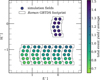
Fig. 1 Layout of the simulation fields, over-plotted on the Roman GBTDS footprint as recommended by the Roman Observations Time Allocation Committee. The colours represent the total number of simulated microlensing events per simulation field over the average for all fields in the run with the PopSyCLE (Lam et al. 2020) default 350 km/s mean NS kick velocity (before applying the detectability cuts).
We converted the PopSyCLE apparent (H, J, K) magnitudes to F146 (using Eq. (1) from Wilson et al. 2023) and applied a F146 < 23 cut. In case of star lenses, this cut was applied to the blended lens+source flux. Using image-level simulations, Wilson et al. (2023) determined F146 = 22 to be the transition at which the background contribution to noise starts exceeding that of the source. We estimate that with tailored data-processing techniques, it should be possible to achieve a drop of ≈1 magnitude below this boundary to obtain scientifically useful images of the source. This is a rough estimate because it is difficult to predict future mission performance; it should be re-evaluated after the Roman start of operations.
We created a set of observing times 𝒯GBTDS that followed the most recent recommendations for the GBTDS survey design, that is, six high-cadence seasons of 70.5 days, centred around the vernal and autumnal equinoxes and filled with 12.1-minute cadence observations, separated in half by a gap of four low-cadence seasons. We also included gap-filling observations every 3 days in the four low-cadence seasons. (This set was the same for all fields, as they will have the same cadence; the choice of a starting point is arbitrary and does not affect the observed event distributions.)
We (conservatively) assumed that to fully characterise the event, we require the closest approach to occur within the bounds of the survey time: min(𝒯GBTDS) < t0 < max(𝒯GBTDS).
To select only events with detectable astrometric signal, we required
![Mathematical equation: $\[\Delta_{ast}>\sigma_{ast} / \sqrt{N}\]$](/articles/aa/full_html/2026/03/aa58238-25/aa58238-25-eq7.png) , where Δast = max |δ(ti) − δ(tj)| : ti, tj ∈ 𝒯GBTDS. We assumed N = 119 for stacking observations taken within 24 hours. We used Eqs. (4) and (5) to calculate δ(t) : t ∈ 𝒯GBTDS values (in Eq. (4), we assume straight-line motion as parallax deviations are typically very small and, with event parameters t0, u0 distributed randomly, do not significantly affect the population distributions); in case of star lenses, we corrected Δast for blending with the lens. We followed Eq. (14) from Fardeen et al. (2024) to obtain σast [mas] for a single observation as a function of magnitude; this formula is based on a straight-line fit to Roman simulations from Sajadian & Sahu (2023).
, where Δast = max |δ(ti) − δ(tj)| : ti, tj ∈ 𝒯GBTDS. We assumed N = 119 for stacking observations taken within 24 hours. We used Eqs. (4) and (5) to calculate δ(t) : t ∈ 𝒯GBTDS values (in Eq. (4), we assume straight-line motion as parallax deviations are typically very small and, with event parameters t0, u0 distributed randomly, do not significantly affect the population distributions); in case of star lenses, we corrected Δast for blending with the lens. We followed Eq. (14) from Fardeen et al. (2024) to obtain σast [mas] for a single observation as a function of magnitude; this formula is based on a straight-line fit to Roman simulations from Sajadian & Sahu (2023).-
Analogously, to select only events with detectable photometric signal, we required
![Mathematical equation: $\[\Delta_{p h o t}>\sigma_{p h o t} / \sqrt{N}\]$](/articles/aa/full_html/2026/03/aa58238-25/aa58238-25-eq8.png) , where Δphot = max |Δm(ti) − Δm(tj)| : ti, tj ∈ 𝒯GBTDS. We used Eqs. (2) and (4) to calculate Δm(t) : t ∈ 𝒯GBTDS values; in case of star lenses, we corrected Δphot for blending with the lens. To obtain σphot for a single observation, we used the relative flux error model depicted in Fig. 4 from Wilson et al. (2023) image simulations and approximated it with a polynomial fit,
, where Δphot = max |Δm(ti) − Δm(tj)| : ti, tj ∈ 𝒯GBTDS. We used Eqs. (2) and (4) to calculate Δm(t) : t ∈ 𝒯GBTDS values; in case of star lenses, we corrected Δphot for blending with the lens. To obtain σphot for a single observation, we used the relative flux error model depicted in Fig. 4 from Wilson et al. (2023) image simulations and approximated it with a polynomial fit,
![Mathematical equation: $\[\begin{aligned}\log _{10}\left(\sigma_F / F\right)= & -1.379 \cdot 10^{-4} m^3+2.817 \cdot 10^{-2} m^2 \\& -7.389 \cdot 10^{-1} m+5.319~[\mathrm{ppt}],\end{aligned}\]$](/articles/aa/full_html/2026/03/aa58238-25/aa58238-25-eq9.png) (6)
(6)where m is the F146 magnitude, and we convert it into magnitudes,
![Mathematical equation: $\[\sigma_{p h o t}=\frac{2.5}{\ln~ 10} \frac{\sigma_F}{F}.\]$](/articles/aa/full_html/2026/03/aa58238-25/aa58238-25-eq10.png) (7)
(7)
After applying all cuts, we retained 2.8% of all simulated events, including 4.8-6.1% (dependent on the kick velocity) of all simulated events with NS lenses. We note that after correcting for blending with luminous lenses, we retained slightly more events (although some that were previously flagged as detectable were lost due to decreased Δphot and Δast, more new lenses were included because they passed the magnitude cut with the increased joint flux). Hereafter, we use ‘detectable’ to describe events passing all cuts, that is, they are both photometrically and astrometrically detectable, unless indicated otherwise. We make datasets containing parameters of these events publicly available in the built-in model library of the popclass classification software5 as gbtds_nskick150, ..., gbtds_nskick450. We also included the full PopSyCLE output for the simulated events in an auxiliary dataset, which we make publicly available on Zenodo. In this dataset, we include the event samples before and after the pre-processing step, in case the users choose to apply their own detectability criteria (e.g. when the Roman performance allows us to relax some cuts in the future).
We did not attempt to assess the constraints that we will be able to make based on the GBTDS data for tE, θE, πE for a given detectable event, and we leave this to future work. Implicitly assumed in the work that follows is that we can measure tE and θE precisely. This assumption was found to be reasonable for the set of events on which we focused. The spur lenses are located at the high-θE end of the parameter space and have tE ~ 10 days, which are likely to be well constrained from the ≈12-minute cadence photometric and astrometric observations of the GBTDS. This point has been documented in several studies. Kaczmarek et al. (2022) found <1% constraints on both tE and θE by modelling simulated GBTDS observations of a nearby NS lensing event. Similarly, Lu et al. (2025) found <1% constraints on tE and <10% on θE by modelling simulated GBTDS observations for an example BH lens. Terry et al. (2025) found that ≈90% of their 3000 simulated GBTDS lenses (chosen to be a representative population of planetary hosts, i.e. systematically lower mass than stellar remnants) have a constraint on tE of ≤10% derived from the light curve alone. On the astrometric front, Sajadian & Sahu (2023) found that >99% of their simulated BH events observed by the GBTDS have a constraint on θE of ≤10%, with the majority of them also having a constraint on tE ≤ 10%, regardless of the mass function assumed. Finally, Fardeen et al. (2024) found that many wide-separation (u0 > 2) events caused by lenses with masses around one solar mass have constraints on θE and tE of <10% from astrometry alone.
In summary, lens parameter constraints from GBTDS observations are a topic of ongoing study, but θE and tE for stellar remnant events are generally expected to be well constrained. We note a key caveat is that these simulations and predictions generally do not consider potential contaminants. Other effects including astrometric binaries (e.g. Jankovič et al. 2025), binary source or binary lens microlensing (e.g. Abrams et al. 2025) can be confused for point source – point lens events, although the extent to which this will affect simultaneous photometric and astrometric observations of GBTDS is yet unclear. Assuming no contamination makes the following work an optimistic upper bound in this respect.
4 Results
4.1 Detectable event yields
To calculate the detectable event yield expected from GBTDS, we upscaled the retained event counts from Sect. 3.3 by SGBTDS/Ssim, the ratio of the full GBTDS footprint area to the total area of simulation fields (depicted in Fig. 1). We assumed Poisson noise on the retained event counts. We note that all reported error bars on event yields only reflect the Poisson noise of the simulation run and not any uncertainties in the Galactic parameters of the underlying simulation. We estimate that GBTDS will include ≈11 000 detectable events overall, including 8710 ± 160 stars and 2229 ± 79 WDs.
Our treatment of massive remnants was more complex. With out-of-the-box simulation results, we retained 168 ± 22 detectable BH events and 254 ± 27, 280 ± 28, 412 ± 34, and 398 ± 33 detectable NS events for vkick of 150, 250, 350, and 450 km/s, respectively. However, these yields are likely to be overestimated. Sweeney et al. (2022) have studied the expected Galactic distributions of stellar remnants, finding NSs and BHs to have more diffuse spatial distributions than the visible Galaxy, primarily because natal kicks change their Galactic orbits. As PopSyCLE currently does not include this effect and keeps the remnants at fixed Galactic positions, the yields we obtained in the simulations described are effectively upper limits (i.e. the yields assume that all NSs are young and have not yet had time to migrate outwards).
We aim to provide more realistic yields by applying a reweighting to our simulated events. We used a sample of 105 simulated NSs from Sweeney et al. (2022) to model the prekick NS distribution. We used the StellarMortis software6 (Sweeney 2025), which assigns kicks to remnants and propagates them in the Milky Way potential to a present-day distribution. We modified StellarMortis to include flexible Maxwellian kick distributions for a given ![Mathematical equation: $\[\bar{v}\]$](/articles/aa/full_html/2026/03/aa58238-25/aa58238-25-eq12.png) and generated four samples of 105 post-kick NSs matching our four simulated kick distributions. We then binned these samples in galactocentric r and |z| (assuming the distributions are axisymmetric and symmetric in z) to minimize random noise. To each simulated NS lens i located at ri, zi, we assigned a weight wi = Npost(ri, |zi|)/Npre(ri, |zi|), which is equal to the ratio of post-kick to pre-kick NS counts in a given bin. Then, our density-corrected yields were equal to the sum ∑i wi · SGBTDS/Ssim over all NS lenses in the simulation. We visualise the NS yields as a function of vkick in Fig. 2 for the weighted and unweighted case. The corrected yields are 181 ± 19, 131 ± 13, 122 ± 10, and 75 ± 6 with increasing vkick. The weighting and its limitations are discussed in more detail in Sect. 5.
and generated four samples of 105 post-kick NSs matching our four simulated kick distributions. We then binned these samples in galactocentric r and |z| (assuming the distributions are axisymmetric and symmetric in z) to minimize random noise. To each simulated NS lens i located at ri, zi, we assigned a weight wi = Npost(ri, |zi|)/Npre(ri, |zi|), which is equal to the ratio of post-kick to pre-kick NS counts in a given bin. Then, our density-corrected yields were equal to the sum ∑i wi · SGBTDS/Ssim over all NS lenses in the simulation. We visualise the NS yields as a function of vkick in Fig. 2 for the weighted and unweighted case. The corrected yields are 181 ± 19, 131 ± 13, 122 ± 10, and 75 ± 6 with increasing vkick. The weighting and its limitations are discussed in more detail in Sect. 5.
The BH kick distribution is very uncertain. BHs are usually expected to have a similar kick momentum distribution as NSs, and they are therefore expected to have lower velocities (e.g. Fryer & Kalogera 2001). However, Repetto et al. (2012) found evidence that the BH kick velocities are similar to those of NSs, and Janka (2013) offered a theoretical mechanism that could explain them. Nagarajan & El-Badry (2025) found evidence for strong kicks for some BHs and weak to none evidence for others with Gaia Data Release 3 kinematics. We note that several recent works on newly discovered BHs support the low-kick hypothesis (e.g. Kotko et al. 2024; Koshimoto et al. 2024; Burdge et al. 2024). For consistency with the PopSyCLE default settings used in our simulations, we assumed vkick = 100 km/s for BHs to apply the same yield correction as for NS lenses. As there are only 75 235 BHs in the Sweeney et al. (2022) remnant sample, we used the full sample to generate weights, resulting in a corrected yield of 152 ± 21 BH lens events.
As the recommended GBTDS strategy is not yet final, we also estimated the detectable event yield assuming no gap-filling (low-cadence) observations. We found that without these observations, we only retained 62% of the detectable events (60% for star lenses, 66% for WD lenses, and 91% for BH lenses). Dependent on vkick, we also retained 72, 66, 62, and 55% of NS events (for vkick of 150, 250, 350, and 450 km/s, respectively)7. Removing the gap-filling observations affects the remnant detections (and especially BH detections) less, as populations of high-mass lenses have longer typical timescales. Strongly kicked NSs are the exception, as high relative lens-source motions cancel this effect out. This experiment proves the effectiveness of gap-filling observations in GBTDS, which can increase the detectable event yield by ≳50% at a relatively low observing time cost (only one hour of observations per three days outside the high-cadence seasons8).
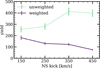 |
Fig. 2 Yield of events with NS lenses detectable with Roman in photometry and astrometry over the entire GBTDS duration as a function of mean kick velocity vkick before (dotted green) and after (solid purple) applying the effect of natal kicks on the volume density of NSs in the Galaxy. The error bars represent the Poisson noise; the |
![Mathematical equation: $\[\sigma^{2}={\sum}_{i} ~w_{i}^{2}\]$](/articles/aa/full_html/2026/03/aa58238-25/aa58238-25-eq11.png)
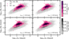 |
Fig. 3 Distributions of NS (purple) and non-NS (grey) events in log10 tE–log10 θE space. All simulated events regardless of whether they passed the detectability cuts are plotted; shade denotes iso-density levels estimated with a Gaussian KDE. The black circles highlight the NS events that passed the detectability cuts. The NS distribution exhibits a characteristic spur feature that becomes stronger and more shifted leftwards with increasing vkick, yielding more detectable NSs that are outliers from the main distribution. |
4.2 Distributions in log10 tE − log10 θE space
With simultaneous photometric and astrometric observations, we can measure three microlensing observables related to the lens mass: tE, θE, and πE. Of these, tE and θE are optimal for remnant classification, as both parameters can be well constrained from observations and increase with lens mass. In contrast, πE is difficult to measure precisely and decreases with lens mass. In photometry, while tE is usually well constrained from the light curve, πE is subject to various degeneracies (Smith et al. 2003; Gould 2004) and is notoriously hard to constrain, especially for remnant candidates (e.g. Kaczmarek et al. 2022; Golovich et al. 2022). In astrometry, for massive remnants (NSs and BHs), the πE contribution is lower by one to two orders of magnitudes than the overall astrometric deviation with which we measure θE. We operate in log–log space as it is optimal for separation of lens classes (e.g. Lam et al. 2020; Fardeen et al. 2024; Kaczmarek et al. 2025).
With increasing vkick, we found an increasing representation of NSs that are outliers from the main distribution in the log10 tE–log10 θE space. In Fig. 3 we plot the simulated event populations in this space, including all NS and non-NS events, regardless of cuts. We show that these outliers are sampled from a continuous spur structure, which is characteristic of the NS population and diagonally offset from the main log10 tE–log10 θE distribution. The region covered by the spur has a high ratio of NSs to total event numbers (for a more detailed discussion and visualisation of the number of NS events and non-NS contaminants expected in this structure, see Figs. 5 and 8 and the corresponding descriptions). We propose using this feature for constructing optimal NS candidate samples.
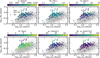 |
Fig. 4 log10 tE–log10 θE space distribution of detectable NS lenses from the vkick = 450 km/s simulation run (coloured) compared to that of lenses from other classes (stars, WDs, and BHs; light grey). The NS lenses are coloured by the event parameters lens velocity vL, lens mass ML, source distance DL, lens distance μL, and a measure of background area subject to light deflection by the lens per unit time θE · μL (from top left row-wise). NSs located in the spur region distinguishable from other lens classes are nearby, have high proper motions, and are relatively very likely to cause lensing events. |
4.3 Properties of detectable NS events
We determined how the physical parameters of NSs are related to their positions in the log10 tE − log10 θE space, and in particular, to their membership in the spur feature. In Fig. 4 we present distributions of several event parameters across the tE − θE space for vkick = 450 km/s, the simulation in which the spur is most prominent.
While weak trends in vL and ML are present (NSs with higher velocities and lower masses on average cause shorter events), neither of these parameters causes the spur. We also note that there is a region that is preferentially occupied by NS events with distant sources at approximately log10 tE = 1.5, log10 θE = 0, which is also unrelated to the spur and not distinguishable from other event classes.
Conversely, in the bottom panels, we present lens parameters that are correlated with membership in the spur. The NS lenses located in the spur are much more nearby and have higher proper motions. We conclude that the spur contains mesolenses, that is, single objects that are naturally high-probability lenses, even though the total contribution to the lensing optical depth from their population may not be very large (Di Stefano 2008a,b). Di Stefano (2008b) stated that mesolenses are caused by a combination of a large Einstein ring, fast angular motion, and a dense background field. For simplicity, we assumed a constant source density within a simulation field, random background source motion, and constant θE per lens. Then, the contribution to the event rate Γ in the field from a single object is ~θE · μL, that is, proportional to the area swept by the Einstein ring per unit time. We plot θE · μL in the bottom right panel, showing that NS lenses located in the spur vastly exceed other NS lenses in their contribution to the event rate, that is, they are very likely to cause lensing events.
These objects are of great interest as they can cause repeated events (e.g. Bramich 2018), allowing high-precision mass determination with several independent mass measurements. To maximise the precision of mass measurements, mesolens candidates should be vetted for possible repeated events. For high-θE events with Roman-like observations, lens motion can be precisely constrained even when the lens is not seen (e.g. Kaczmarek et al. 2022). When the motions of the found mesolenses can be constrained well enough from Roman data, predictions for future events should also be made to enable follow-up observations.
Figure 4 shows the lenses as recovered from the simulation without the correction for Galactic NS density. To visualise the effect of this correction, we also plot the weights and z positions in a supplementary Fig. 5, which shows that the spur lenses have systematically lower weights. This result may seem counter-intuitive because the expansion of the NS distribution will result in lenses migrating from the Bulge to higher galactocentric radii, and therefore, a higher fraction of nearby mesolenses might be expected. However, this is explained by the lower panel: as the line of sight is fixed, the nearby lenses falling into the Roman fields have z ≈ z⊙ ≈ 0. As the postkick NS distributions have inflated scale heights, the weights increase with |z|. Overall, for vkick = 450 km/s, we expect roughly ∑i wi · SGBTDS/Ssim ≈ 6 NS lenses in the spur. Every detection of a lens in the spur region will be extremely valuable for population constraints because the sample size is so small. We suggest that all lenses found in that region of log10 tE–log10 θE space should be preferentially allocated follow-up resources (e.g. spectroscopy for a source characterisation).
To follow up on the correlation between DL and the location in the spur, we present lens distance histograms for all simulations in Fig. 6. We found that the lens distance distribution is dependent on vkick, which makes it useful for constraining the NS kick. While the nearby mesolenses are, again, more affected by down-weighting, high vkick still yield flatter, more tailed lens distance distributions. As in the case of the spur structure, strong kicks affect the strengthening (generating nearby mesolenses) and weakening (preferential drop in density of nearby lenses along a fixed l.o.s. due to their low |z|) of a distinct structure in parameter distribution. Detailed studies of these counteracting effects will be necessary to leverage upcoming data for population constraints.
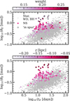 |
Fig. 5 Like Fig. 4, but coloured by parameters relevant to correcting for the changed NS density: weight and galactocentric z coordinate. In the top subplot, black outlines denote events we selected as ‘in spur’ to estimate the total yield of about six expected ‘spur’ NS lenses in GBTDS, assuming vkick = 450 km/s. |
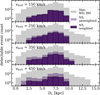 |
Fig. 6 Distributions of detectable NS lens distances for all four runs, with vkick increasing from top to bottom. The unweighted distance distribution is plotted in light purple, and the weighted (with post-kick Galactic density correction) distance distribution is plotted in dark purple with black contours. The distance distribution for all other detectable lenses (classL ∈ {star, WD, BH}) is plotted in light grey. All yields are adjusted to the total survey area. |
4.4 NS classification
In this section, we discuss prospects for distinguishing NS lenses from other classes using their log10 tE–log10 θE distributions. For each of the four simulation runs, we built a classifier returning the lens class probability for a given point or distribution in a subspace of observables as described in Kaczmarek et al. (2025) (we refer to that work for a detailed description of the classification method). In summary, we used the Bayes theorem to define the probability of the lens causing a microlensing event with a set of observable parameters ϕ belonging to classL under a Galactic model 𝒢,
![Mathematical equation: $\[p\left(\operatorname{class}_L {\mid} \phi, \mathcal{G}\right)=\frac{p\left(\operatorname{class}_L {\mid} \mathcal{G}\right) p\left(\phi {\mid} \operatorname{class}_L, \mathcal{G}\right)}{p(\phi {\mid} \mathcal{G})}.\]$](/articles/aa/full_html/2026/03/aa58238-25/aa58238-25-eq13.png) (8)
(8)
We took p(classL|𝒢) directly from the event counts per class in the simulated dataset. To construct continuous p(ϕ|classL, 𝒢) from discrete sampling, we used Gaussian kernel density estimators (KDEs) constructed in the ϕ parameter space with detectable simulated events of a given classL as implemented in scipy (Virtanen et al. 2020) with default settings. We note that Eq. (8) assumes a perfect measurement of the observable parameters ϕ, which makes this analysis optimistic. However, by the very nature of the spur feature being in the high θE portion of the parameter space, the lenses of interest are expected to preferentially skew towards high signal-to-noise ratios, making this assumption less effective than it would normally be for analyses that are focused on the bulk of the observed catalogue. p(ϕ|𝒢) is simply a normalising factor independent of classL, which we applied by ensuring ∑classL p(classL|ϕ, 𝒢) = 1. We made one change compared to Kaczmarek et al. (2025) in that we incorporated NS and BH weights in the creation of the respective KDEs.
To account for the epistemic uncertainty of the classifier in addition to the astrophysical classes {star, WD, NS, BH}, we included the ‘none’ class, which was assigned when the parameters ϕ are not consistent with those of event populations in the underlying simulation (see Sect. 3.3 and Appendix A in Kaczmarek et al. 2025 for a detailed explanation of the none class). The none class was constructed following the formula
![Mathematical equation: $\[p(\phi {\mid} \text {None,} \mathcal{G})=A\left(1-\frac{p(\phi {\mid}\mathcal{G})}{\max _\phi(p(\phi{\mid}\mathcal{G}))}\right),\]$](/articles/aa/full_html/2026/03/aa58238-25/aa58238-25-eq14.png) (9)
(9)
where A is a constant setting the none class weight, and p(ϕ|𝒢) is approximated with a top-hat KDE constructed on the ϕ parameter space with all detectable simulated events, using the scikit-learn (Pedregosa et al. 2011) implementation. We set A to 10−4 and the KDE bandwidth to 0.3. As the none class is designed to represent parameters without support in the simulation samples, the construction of this KDE is not affected by NS or BH weighting.
In practice, we constructed the KDEs on a 1000 × 1000 grid and evaluated p(classL|ϕ, 𝒢) using the nearest grid point. Using this method, we constructed relative probability maps, that is, plots showing the p(classL|ϕ, 𝒢) that would be assigned as a function of event parameters ϕ assuming they are known exactly. We show these probability maps for vkick ∈ (150, 450) km/s in Fig. 7, demonstrating that moving from the space of photometry-only observables (tE, πE) to that of high-signal photometry + astrometry observables (tE, θE) allows for the high-confidence NS classification in case of high vkick. For the photometry-only subplots, we used all events that only passed the magnitude cut and the photometrically detectable signal cut, whereas for the photometry+astrometry subplots, we used events passing all Sect. 3.3 cuts, also including the astrometrically detectable signal cut.
To test prospects for constructing NS samples with this classifier, we used threshold probabilities plim: we included a simulated event with parameters ϕ in our sample when p(classL|ϕ, 𝒢) > plim. We constructed these samples for all simulation runs and for several thresholds: plim ∈ (0.05, 0.1, 0.3, 0.5). We then corrected our included and total event counts for NS and BH weights. We illustrate the count of retained NS events, recall, and purity in this experiment in Fig. 8.
Samples constructed using a very low plim = 0.05 have consistently high (0.3 − 0.4) recall, but at a cost of low (0.1 − 0.2) purity. Still, we note that this fraction of NSs within the sample is larger by one to two orders of magnitude than in the entire dataset. These samples contain several dozen NSs and are selected from the spur and surrounding regions. Conversely, samples constructed using plim ∈ {0.3, 0.5} contain only NSs, but at a cost of low recall (<10 events). These samples were selected from the far side of the spur; for lower vkick, they cannot be constructed as there is no region in the parameter space that is sufficiently unique to NSs.
We note that membership in the NS lens class can be verified independently, for instance with the lens mass being consistent with an NS mass and the non-detection of additional blended light expected from a luminous (e.g. main-sequence) star of the determined lens mass and distance. Therefore, the above exercise can be interpreted as constructing a sample of promising candidates that should be allocated additional analysis and observation resources, similarly to BH lens candidates in Kaczmarek et al. (2025). In this situation, thresholds should be determined by adjusting the sample size to the available resources.
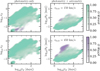 |
Fig. 7 Left: relative class probabilities in log10 tE–log10 πE, i.e. the space of observables that is accessible from photometric observations alone. The probability map was constructed using all photometrically detectable events. Right: relative class probabilities in log10 tE–log10 θE, i.e. the space of observables that can be measured with high precision with the combination of photometry and astrometry. The probability map was constructed using all photometrically and astrometrically detectable events. Each relative probability map is presented for vkick = 150 km/s (top) and 450 km/s (bottom). High vkick results in a parameter distribution that is more distinguishable from other lens classes. In particular, in the log10 tE–log10 θE space, there is a region preferentially occupied by NSs, which reaches p(NS|ϕ, 𝒢) ≈ 1 and could be used for constructing optimal samples of isolated NS candidates. (For clarity, the WD and BH lens class probabilities are not plotted, as the Star class is the main source of confusion with the NS class.) |
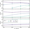 |
Fig. 8 Top: count of retained NS events within an event sample constructed using a given plim, rescaled to yields from the full GBTDS footprint. The error bars representing Poisson noise are the same as in Fig. 2. Centre: recall of NS events, calculated as a ratio of selected NS events to all detectable NS events. Bottom: purity of the sample, calculated as a ratio of selected NS events to all events selected for the sample. For higher plim, values for vkick ∈ (150, 250) km/s are missing as samples cannot be constructed (i.e. the resulting sample size is 0). |
5 Discussion and conclusions
We have conducted simulations of gravitational microlensing events tailored to the most recent proposed Roman Space Telescope GBTDS design. We specifically focused on NS lenses, which are very hard to identify with the instrumentation constraints of current microlensing surveys because they are easily confused with other lens classes, but will become discoverable with Roman. To assess the effect of NS natal kicks on microlensing observables, we ran four simulations with Maxwellian kick distributions in which we varied the mean kick velocity vkick.
We found that distributions of microlensing observables differ for NS populations with different vkick. In the log10 tE–log10 θE space, which is favourable for a remnant classification, we found a feature that is uniquely characteristic of NS lenses: a spur that is diagonally offset from the main distribution towards lower tE and higher θE. The strength and exact location of this structure varies with vkick, making it most distinct at the high end, vkick = 450 km/s.
We identified the spur NSs as mesolenses, which is a class of nearby fast objects that have a high probability of causing lensing events and might even cause repeated events. Strong kicks cause both effects to strengthen the spur (increased potential for generating mesolenses) and to weaken it (decreased NS density), which makes it especially challenging to study this structure and use it for drawing constraints on the kick distributions. Detailed studies including careful modelling of NS dynamics, larger sample sizes, and more kick velocity distributions are needed.
We note that if the NS spur feature is detectable in real Roman observations, it might enable the identification of highly likely NS candidates without requiring a πE, which may represent a bottleneck for full lens characterisation in GBTDS microlensing events. We therefore recommend that all events found in this region should be treated with special care and allocated necessary follow-up resources by prioritising their ingestion into Target and Observation management systems (e.g. Street et al. 2018; Coulter et al. 2023) so they can be tracked and this new potential characterisation pathway can be investigated.
We predict that Roman will find approximately 11 000 microlensing events that are detectable in both photometry and astrometry, ~100 of which will be isolated NSs. With direct mass measurements available via a complete resolution of microlensing parameters, this dataset will provide outstanding statistical constraints on the NS EoS and the speculated mass gap. In total, this dataset will contain approximately 2500 compact objects, providing an unprecedented census of isolated stellar remnants. While in this work, we focused on NS classification and population properties, we note that the GBTDS-tailored simulation results will also be useful for other science cases, and we make them publicly available within the popclass classification software and in the auxiliary Zenodo dataset.
We note that this study is constrained by several limitations. All predictions about Roman concerning the survey strategy and instrument performance are preliminary and will need to be verified in the later stages of the mission. Furthermore, a simulation can only be as accurate as the underlying Galactic model. PopSyCLE relies on dedicated models of the Milky Way and stellar evolution. However, some questions about the Galactic structure remain open, including the bar angle and pattern speed and the mass distribution (e.g. Hunt & Vasiliev 2025). There are even more unknowns regarding the creation of remnants. We assumed a single Maxwellian distribution for natal kicks, while more complex distributions are also discussed. Igoshev (2020) propose a bimodal kick distribution, for example. The IFMR between progenitors and remnants is poorly known; it is difficult to test (especially in the mass-gap range) due to the obstacles and biases in remnant detection and mass measurement discussed in Sect. 1. Various initial-final mass prescriptions, using different methods, have been proposed in the literature (see Rose et al. 2022 for a detailed description of IFMRs integrated into PopSyCLE and their effect on microlensing).
Notably, Sweeney et al. (2022) have demonstrated with simulations that the spatial Galactic distribution of NSs should be more diffuse than that of other astrophysical classes because their progenitors experience the evolving structure of the Galaxy and because their post-kick orbits change. However, PopSyCLE currently does not model the latter. For a more detailed discussion of the effect of this limitation on microlensing predictions, we refer to Lam et al. (2020).
We attempted to correct for this effect in the post-processing. Namely, we ran dynamical simulations for 105 simulated prekick NSs sampled from the Sweeney et al. (2022) dataset to obtain four post-kick present-day Galactic distributions of NSs. We used the StellarMortis software (Sweeney 2025), which was developed as part of the Sweeney et al. (2022) work. We approximated post-kick to pre-kick density ratios for a given vkick and galactocentric position by bin count ratios. We then assigned weights to our simulated NSs to correct for the changed densities. This correction lowered the total yields by a factor of 1.4 (lowest vkick) to 5.3 (highest vkick).
Our treatment of massive remnants was similar to that of most recent microlensing studies of BH natal kicks. Koshimoto et al. (2024) accounted for the changed remnant distributions by modifying the Galactic model of Koshimoto et al. (2021) with an analytical scale height and surface density profiles fitted to the numerical results of Tsuna et al. (2018). They then generated BH lenses following the prescription (IFMR and adding kicks) of Lam et al. (2020). They found a similar trend of increasing BH yields (represented as a fractional contribution per tE bin) with increasing vkick when not applying disk inflation, but decreasing after this correction of the model. In the final stages of preparing this work, a pre-print by Wu et al. (2026) has been made available that discusses BH selection and event rates from a combination of ground-based microlensing surveys and interferometry. Wu et al. (2026) correct for BH kick effects by applying weight factors to their expected event rates separately for the disk (where they follow the analytical formulae of Koshimoto et al. 2024) and the bulge (which they model as an exponential distribution whose effective radius changes with kick velocity, assuming a steady state).
We note that the solution of applying the weights we used in this work is not perfect. While the first-order effect of dynamical evolution is the changed NS density, we also expect velocity distributions to be affected as the NS orbits change. This effect is very difficult to model and cannot be handled with a simple correcting factor because present-day NS velocity distributions are expected to vary with Galactic position and age (see e.g. Fig. 3 in Sweeney et al. 2022). Clearly, it would be ideal to have a fully realistic population of NSs with present-day positions and velocities available to use as lenses. However, to create such a population, we would need to consider that the NSs are created in a different Galactic position, that is, at a different line of sight, than they are observed as lenses. This is incompatible with the way PopSyCLE works, which includes a computationally expensive population synthesis of stars along a chosen line of sight to simulate small circular fields (see e.g. Fig. 1). A full simulation including the dynamical evolution of NSs across all possible lines of sight, that is, the entire Galaxy, would be extremely computationally expensive. For example, even without simulating microlensing, Sweeney et al. (2022) needed to apply a down-sampling of the remnant and star populations by 103 and 106, respectively, to make the aforementioned study computationally feasible. Such a down-sampling would be far from sufficient for studying parameter distributions or estimating yields for a survey such as GBTDS. PopSyCLE, considering all NSs in a given pencil beam without down-sampling, only returns ~102 NS lens yields in our simulations. Finally, we note that our weighting factors assumed axisymmetry; indeed, our simulated samples of post-kick NS are well described by an axisymmetric distribution, as Sweeney et al. (2022) and StellarMortis did not include non-axisymmetric components (e.g. a bar) of the Milky Way potential.
However, as high-performance clusters and simulation codes develop exponentially, it is conceivable that microlensing simulations are no longer hindered by these computational limitations in the near future. We have outlined some areas of focus that might be useful for such a future study. Other limitations discussed above might also be alleviated in the coming years with the start of Roman operations, Galactic models informed by new surveys, including the upcoming Gaia data releases, and improvements in stellar evolution codes.
Regardless of these limitations, we made promising observations on the Roman isolated NS population. We found a feature in the observable parameter space that is characteristic of NSs. The shape and strength of this feature is dependent on NS kicks. Hence, it can be leveraged to constrain natal kick distributions. Similarly, the distance distribution of NS lenses is also dependent on NS kicks. We found that strong kicks exhibit effects that both strengthen (via high NS velocities) and weaken (via decreased NS density, especially at low |z|) these characteristic features. The interplay of these effects should be treated with special care and should ideally be studied with dedicated simulations focusing on NS dynamics in the future.
In the course of this work, we produced simulations extending beyond the NS population. We also extended the popclass classification software (Sallaberry et al. 2025) to include our simulation results in anticipation of GBTDS. We provide expected yields of events detectable by Roman for each of the astrophysical lens classes (stars, WDs, NSs, and BHs). We demonstrated the effect of the survey strategy and detectability criteria on the event yields, and we make all simulated events available with detectability flags so that these criteria can be further analysed and adjusted. All microlensing event datasets generated in this study are publicly available.
Acknowledgements
The authors acknowledge support by the state of Baden-Württemberg through bwHPC. We would like to thank Joachim Wambsganss, David Sweeney, Oskar Grocholski, Jessica Lu, Macy Huston, and Natasha Abrams for useful discussions. We thank the anonymous reviewer for their comments that helped improve the quality of this paper. This work was performed under the auspices of the U.S. Department of Energy by Lawrence Livermore National Laboratory under Contract DE-AC52-07NA27344. The document number is LLNL-JRNL-2013705. This work was supported by the LLNL LDRD Program under Project 22-ERD-037.
References
- Abbott, B. P., Abbott, R., Abbott, T. D., et al. 2017, Phys. Rev. Lett., 119, 161101 [Google Scholar]
- Abbott, B. P., Abbott, R., Abbott, T. D., et al. 2020, ApJ, 892, L3 [NASA ADS] [CrossRef] [Google Scholar]
- Abbott, R., Abbott, T. D., Abraham, S., et al. 2021, Phys. Rev. X, 11, 021053 [Google Scholar]
- Abrams, N. S., Lu, J. R., Lam, C. Y., et al. 2025, ApJ, 980, 103 [Google Scholar]
- Annala, E., Gorda, T., Kurkela, A., Nättilä, J., & Vuorinen, A. 2020, Nat. Phys., 16, 907 [NASA ADS] [CrossRef] [Google Scholar]
- Annala, E., Gorda, T., Hirvonen, J., et al. 2023, Nat. Comm., 14, 8451 [Google Scholar]
- Bailyn, C. D., Jain, R. K., Coppi, P., & Orosz, J. A. 1998, ApJ, 499, 367 [NASA ADS] [CrossRef] [Google Scholar]
- Barlow, R. 1987, J. Comput. Phys., 72, 202 [Google Scholar]
- Baym, G., Hatsuda, T., Kojo, T., et al. 2018, Rep. Prog. Phys., 81, 056902 [NASA ADS] [CrossRef] [Google Scholar]
- Belczynski, K., Wiktorowicz, G., Fryer, C. L., Holz, D. E., & Kalogera, V. 2012, ApJ, 757, 91 [NASA ADS] [CrossRef] [Google Scholar]
- Bell Burnell, J. 2017, Nat. Astron., 1, 831 [Google Scholar]
- Bhattacharyya, S. 2010, Adv. Space Res., 45, 949 [Google Scholar]
- Bramich, D. M. 2018, A&A, 618, A44 [NASA ADS] [CrossRef] [EDP Sciences] [Google Scholar]
- Bray, J. C., & Eldridge, J. J. 2016, MNRAS, 461, 3747 [NASA ADS] [CrossRef] [Google Scholar]
- Burdge, K. B., El-Badry, K., Kara, E., et al. 2024, Nature, 635, 316 [NASA ADS] [CrossRef] [Google Scholar]
- Chatziioannou, K., Cromartie, H. T., Gandolfi, S., et al. 2025, Rev. Mod. Phys., 97, 045007 [Google Scholar]
- Coulter, D. A., Jones, D. O., McGill, P., et al. 2023, PASP, 135, 064501 [Google Scholar]
- Damineli, A., Almeida, L. A., Blum, R. D., et al. 2016, MNRAS, 463, 2653 [NASA ADS] [CrossRef] [Google Scholar]
- DeRocco, W., Frangipane, E., Hamer, N., Profumo, S., & Smyth, N. 2024, Phys. Rev. D, 109, 023013 [Google Scholar]
- Di Stefano, R. 2008a, ApJ, 684, 59 [Google Scholar]
- Di Stefano, R. 2008b, ApJ, 684, 46 [Google Scholar]
- Disberg, P., Gaspari, N., & Levan, A. J. 2025, A&A, 700, A75 [NASA ADS] [CrossRef] [EDP Sciences] [Google Scholar]
- Dominik, M., & Sahu, K. C. 2000, ApJ, 534, 213 [CrossRef] [Google Scholar]
- El-Badry, K., Rix, H.-W., Latham, D. W., et al. 2024, Open J. Astrophys., 7, 58 [Google Scholar]
- Fardeen, J., McGill, P., Perkins, S. E., et al. 2024, ApJ, 965, 138 [Google Scholar]
- Farr, W. M., Sravan, N., Cantrell, A., et al. 2011, ApJ, 741, 103 [NASA ADS] [CrossRef] [Google Scholar]
- Fonseca, E., Cromartie, H. T., Pennucci, T. T., et al. 2021, ApJ, 915, L12 [NASA ADS] [CrossRef] [Google Scholar]
- Fortin, F., García, F., Chaty, S., Chassande-Mottin, E., & Simaz Bunzel, A. 2022, A&A, 665, A31 [NASA ADS] [CrossRef] [EDP Sciences] [Google Scholar]
- Fraga, E. S., Kurkela, A., & Vuorinen, A. 2016, Euro. Phys. J. A, 52, 49 [Google Scholar]
- Fryer, C. L., & Kalogera, V. 2001, ApJ, 554, 548 [Google Scholar]
- Giacobbo, N., & Mapelli, M. 2020, ApJ, 891, 141 [NASA ADS] [CrossRef] [Google Scholar]
- Golovich, N., Dawson, W., Bartolić, F., et al. 2022, ApJS, 260, 2 [Google Scholar]
- Gould, A. 2004, ApJ, 606, 319 [NASA ADS] [CrossRef] [Google Scholar]
- Gunn, J. E., & Ostriker, J. P. 1970, ApJ, 160, 979 [NASA ADS] [CrossRef] [Google Scholar]
- Haensel, P., Potekhin, A. Y., & Yakovlev, D. G. 2007, Neutron Stars 1: Equation of State and Structure, (New York, USA: Springer), 326 [Google Scholar]
- Harding, A. J., Stefano, R. D., Lépine, S., et al. 2018, MNRAS, 475, 79 [Google Scholar]
- Hewish, A., Bell, S. J., Pilkington, J. D. H., Scott, P. F., & Collins, R. A. 1968, Nature, 217, 709 [NASA ADS] [CrossRef] [Google Scholar]
- Hobbs, G., Lorimer, D. R., Lyne, A. G., & Kramer, M. 2005, MNRAS, 360, 974 [Google Scholar]
- Hog, E., Novikov, I. D., & Polnarev, A. G. 1995, A&A, 294, 287 [NASA ADS] [Google Scholar]
- Hosek, Matthew W., J., Lu, J. R., Lam, C. Y., et al. 2020, AJ, 160, 143 [NASA ADS] [CrossRef] [Google Scholar]
- Howil, K., Wyrzykowski, Ł., Kruszyńska, K., et al. 2025, A&A, 694, A94 [NASA ADS] [CrossRef] [EDP Sciences] [Google Scholar]
- Hunt, J. A. S., & Vasiliev, E. 2025, New A Rev., 100, 101721 [Google Scholar]
- Husseiniova, A., McGill, P., Smith, L. C., & Evans, N. W. 2021, MNRAS, 506, 2482 [Google Scholar]
- Igoshev, A. P. 2020, MNRAS, 494, 3663 [NASA ADS] [CrossRef] [Google Scholar]
- Igoshev, A. P., Chruslinska, M., Dorozsmai, A., & Toonen, S. 2021, MNRAS, 508, 3345 [NASA ADS] [CrossRef] [Google Scholar]
- Janka, H.-T. 2013, MNRAS, 434, 1355 [Google Scholar]
- Janka, H.-T. 2017, ApJ, 837, 84 [Google Scholar]
- Janka, H.-T., & Kresse, D. 2024, Ap&SS, 369, 80 [NASA ADS] [CrossRef] [Google Scholar]
- Jankovič,, T., Gomboc, A., Wyrzykowski, Ł., et al. 2025, A&A, 699, A156 [NASA ADS] [CrossRef] [EDP Sciences] [Google Scholar]
- Ji, Z., Chen, J., & Chen, Y. 2025, arXiv e-prints [arXiv:2505.05241] [Google Scholar]
- Johnson, S. A., Penny, M., Gaudi, B. S., et al. 2020, AJ, 160, 123 [NASA ADS] [CrossRef] [Google Scholar]
- Kaczmarek, Z., McGill, P., Evans, N. W., et al. 2022, MNRAS, 514, 4845 [CrossRef] [Google Scholar]
- Kaczmarek, Z., McGill, P., Perkins, S. E., et al. 2025, ApJ, 981, 183 [Google Scholar]
- Kalogera, V., Kolb, U., & King, A. R. 1998, ApJ, 504, 967 [NASA ADS] [CrossRef] [Google Scholar]
- Kapil, V., Mandel, I., Berti, E., & Müller, B. 2023, MNRAS, 519, 5893 [NASA ADS] [CrossRef] [Google Scholar]
- Kim, S.-L., Lee, C.-U., Park, B.-G., et al. 2016, J. Korean Astron. Soc., 49, 37 [Google Scholar]
- Kim, M., Kim, Y.-M., Sung, K. H., Lee, C.-H., & Kwak, K. 2021, A&A, 650, A139 [NASA ADS] [CrossRef] [EDP Sciences] [Google Scholar]
- Koehn, H., Rose, H., Pang, P. T. H., et al. 2025, Phys. Rev. X, 15, 021014 [Google Scholar]
- Koshimoto, N., Baba, J., & Bennett, D. P. 2021, ApJ, 917, 78 [NASA ADS] [CrossRef] [Google Scholar]
- Koshimoto, N., Kawanaka, N., & Tsuna, D. 2024, ApJ, 973, 5 [Google Scholar]
- Kotko, I., Banerjee, S., & Belczynski, K. 2024, MNRAS, 535, 3577 [Google Scholar]
- Kumar, R., Dexheimer, V., Jahan, J., et al. 2024, Liv. Rev. Relativ., 27, 3 [Google Scholar]
- Lai, D. 2004, in Cosmic Explosions in Three Dimensions, eds. P. Höflich, P. Kumar, & J. C. Wheeler (Cambridge, UK: Cambridge University Press), 276 [Google Scholar]
- Lam, C. Y., Lu, J. R., Hosek, Matthew W., J., Dawson, W. A., & Golovich, N. R. 2020, ApJ, 889, 31 [NASA ADS] [CrossRef] [Google Scholar]
- Lam, C. Y., Lu, J. R., Udalski, A., et al. 2022a, ApJ, 933, L23 [NASA ADS] [CrossRef] [Google Scholar]
- Lam, C. Y., Lu, J. R., Udalski, A., et al. 2022b, ApJS, 260, 55 [Google Scholar]
- Lam, C. Y., Abrams, N., Andrews, J., et al. 2023, arXiv e-prints [arXiv:2306.12514] [Google Scholar]
- Lattimer, J. M. 2012, Ann. Rev. Nucl. Part. Sci., 62, 485 [NASA ADS] [CrossRef] [Google Scholar]
- Lattimer, J. M. 2021, Ann. Rev. Nucl. Part. Sci., 71, 433 [NASA ADS] [CrossRef] [Google Scholar]
- Lattimer, J. M., & Prakash, M. 2004, Science, 304, 536 [NASA ADS] [CrossRef] [Google Scholar]
- Lu, J. R., Medford, M., Lam, C. Y., et al. 2025, AAS Journals, submitted [arXiv:2512.03364] [Google Scholar]
- Lu, X., & Xie, Y. 2024, ApJ, 962, 56 [Google Scholar]
- Lyne, A. G., & Lorimer, D. R. 1994, Nature, 369, 127 [NASA ADS] [CrossRef] [Google Scholar]
- Malik, T., Pais, H., & Providência, C. 2024, A&A, 689, A242 [NASA ADS] [CrossRef] [EDP Sciences] [Google Scholar]
- Mandel, I., & Müller, B. 2020, MNRAS, 499, 3214 [NASA ADS] [CrossRef] [Google Scholar]
- McGill, P., Anderson, J., Casertano, S., et al. 2023, MNRAS, 520, 259 [NASA ADS] [CrossRef] [Google Scholar]
- Miyamoto, M., & Yoshii, Y. 1995, AJ, 110, 1427 [NASA ADS] [CrossRef] [Google Scholar]
- Mróz, P., Udalski, A., & Gould, A. 2022, ApJ, 937, L24 [CrossRef] [Google Scholar]
- Mróz, P., Udalski, A., Szymański, M. K., et al. 2020, ApJS, 249, 16 [CrossRef] [Google Scholar]
- Nagarajan, P., & El-Badry, K. 2025, PASP, 137, 034203 [Google Scholar]
- O’Doherty, T. N., Bahramian, A., Miller-Jones, J. C. A., et al. 2023, MNRAS, 521, 2504 [CrossRef] [Google Scholar]
- Ofek, E. O. 2018, ApJ, 866, 144 [Google Scholar]
- Ono, K., Eda, K., & Itoh, Y. 2015, Phys. Rev. D, 91, 084032 [Google Scholar]
- Özel, F., Psaltis, D., Narayan, R., & McClintock, J. E. 2010, ApJ, 725, 1918 [CrossRef] [Google Scholar]
- Paczynski, B. 1991, ApJ, 371, L63 [CrossRef] [Google Scholar]
- Paczynski, B. 1996, ARA&A, 34, 419 [NASA ADS] [CrossRef] [Google Scholar]
- Pedregosa, F., Varoquaux, G., Gramfort, A., et al. 2011, J. Mach. Learn. Res., 12, 2825 [Google Scholar]
- Penny, M. T., Gaudi, B. S., Kerins, E., et al. 2019, ApJS, 241, 3 [CrossRef] [Google Scholar]
- Perkins, S. E., McGill, P., Dawson, W., et al. 2024, ApJ, 961, 179 [Google Scholar]
- Piffl, T., Scannapieco, C., Binney, J., et al. 2014, A&A, 562, A91 [CrossRef] [EDP Sciences] [Google Scholar]
- Podsiadlowski, P., Pfahl, E., & Rappaport, S. 2005, ASP Conf. Ser., 328, 327 [Google Scholar]
- Pruett, K., Dawson, W., Medford, M. S., et al. 2024, ApJ, 970, 169 [Google Scholar]
- Rawls, M. L., Orosz, J. A., McClintock, J. E., et al. 2011, ApJ, 730, 25 [NASA ADS] [CrossRef] [Google Scholar]
- Reardon, D. J., Hobbs, G., Coles, W., et al. 2016, MNRAS, 455, 1751 [NASA ADS] [CrossRef] [Google Scholar]
- Repetto, S., Davies, M. B., & Sigurdsson, S. 2012, MNRAS, 425, 2799 [Google Scholar]
- Robin, A. C., Reylé, C., Derrière, S., & Picaud, S. 2004, A&A, 416, 157 [NASA ADS] [CrossRef] [EDP Sciences] [Google Scholar]
- Romani, R. W., Kandel, D., Filippenko, A. V., Brink, T. G., & Zheng, W. 2022, ApJ, 934, L17 [NASA ADS] [CrossRef] [Google Scholar]
- Rose, S., Lam, C. Y., Lu, J. R., et al. 2022, ApJ, 941, 116 [Google Scholar]
- Rybicki, K. A., Wyrzykowski, Ł., Klencki, J., et al. 2018, MNRAS, 476, 2013 [NASA ADS] [CrossRef] [Google Scholar]
- Sahu, K. C., Anderson, J., Casertano, S., et al. 2017, Science, 356, 1046 [Google Scholar]
- Sahu, K. C., Anderson, J., Casertano, S., et al. 2022, ApJ, 933, 83 [Google Scholar]
- Sajadian, S., & Sahu, K. C. 2023, AJ, 165, 96 [Google Scholar]
- Sallaberry, G., Kaczmarek, Z., McGill, P., et al. 2025, J. Open Source Softw., 10, 7769 [Google Scholar]
- Schwarz, D. J., & Seidel, D. 2002, A&A, 388, 483 [NASA ADS] [CrossRef] [EDP Sciences] [Google Scholar]
- Shao, Y. 2022, Res. Astron. Astrophys., 22, 122002 [CrossRef] [Google Scholar]
- Sharma, S., Bland-Hawthorn, J., Johnston, K. V., & Binney, J. 2011, ApJ, 730, 3 [NASA ADS] [CrossRef] [Google Scholar]
- Shin, I.-G., Yee, J. C., Zang, W., et al. 2024, AJ, 167, 269 [NASA ADS] [CrossRef] [Google Scholar]
- Smith, M. C., Mao, S., & Paczyński, B. 2003, MNRAS, 339, 925 [NASA ADS] [CrossRef] [Google Scholar]
- Somasundaram, R., Tews, I., & Margueron, J. 2023, Phys. Rev. C, 107, 025801 [CrossRef] [Google Scholar]
- Spergel, D., Gehrels, N., Baltay, C., et al. 2015, arXiv e-prints [arXiv:1503.03757] [Google Scholar]
- Stone, R. C. 1982, AJ, 87, 90 [Google Scholar]
- Street, R. A., Bowman, M., Saunders, E. S., & Boroson, T. 2018, SPIE Conf. Ser., 10707, 1070711 [Google Scholar]
- Sukhbold, T., & Woosley, S. E. 2014, ApJ, 783, 10 [NASA ADS] [CrossRef] [Google Scholar]
- Sukhbold, T., Ertl, T., Woosley, S. E., Brown, J. M., & Janka, H. T. 2016, ApJ, 821, 38 [NASA ADS] [CrossRef] [Google Scholar]
- Sumi, T., Bennett, D. P., Bond, I. A., et al. 2013, ApJ, 778, 150 [Google Scholar]
- Sweeney, D. 2025, https://doi.org/10.5281/zenodo.17970197 [Google Scholar]
- Sweeney, D., Tuthill, P., Sharma, S., & Hirai, R. 2022, MNRAS, 516, 4971 [NASA ADS] [CrossRef] [Google Scholar]
- Tauris, T. M., Fender, R. P., van den Heuvel, E. P. J., Johnston, H. M., & Wu, K. 1999, MNRAS, 310, 1165 [NASA ADS] [CrossRef] [Google Scholar]
- Taylor, J. H., Fowler, L. A., & McCulloch, P. M. 1979, Nature, 277, 437 [NASA ADS] [CrossRef] [Google Scholar]
- Terry, S. K., Bachelet, E., Zohrabi, F., et al. 2025, AJ, submitted [arXiv:2510.13974] [Google Scholar]
- Tsuna, D., Kawanaka, N., & Totani, T. 2018, MNRAS, 477, 791 [NASA ADS] [CrossRef] [Google Scholar]
- Udalski, A., Szymański, M. K., & Szymański, G. 2015, Acta Astron., 65, 1 [NASA ADS] [Google Scholar]
- Virtanen, P., Gommers, R., Oliphant, T. E., et al. 2020, Nat. Methods, 17, 261 [Google Scholar]
- Walker, M. A. 1995, ApJ, 453, 37 [NASA ADS] [CrossRef] [Google Scholar]
- Wilson, R. F., Barclay, T., Powell, B. P., et al. 2023, ApJS, 269, 5 [Google Scholar]
- Woosley, S. E. 2017, ApJ, 836, 244 [Google Scholar]
- Woosley, S. E., Sukhbold, T., & Janka, H. T. 2020, ApJ, 896, 56 [NASA ADS] [CrossRef] [Google Scholar]
- Wu, Z., Dong, S., Gould, A. P., Mróz, P., & Mérand, A. 2026, ApJ, 997, 63 [Google Scholar]
- Wyrzykowski, Ł., & Mandel, I. 2020, A&A, 636, A20 [NASA ADS] [CrossRef] [EDP Sciences] [Google Scholar]
- Wyrzykowski, Ł., Kostrzewa-Rutkowska, Z., Skowron, J., et al. 2016, MNRAS, 458, 3012 [NASA ADS] [CrossRef] [Google Scholar]
- Zevin, M., Spera, M., Berry, C. P. L., & Kalogera, V. 2020, ApJ, 899, L1 [Google Scholar]
- Zurlo, A., Gratton, R., Mesa, D., et al. 2018, MNRAS, 480, 236 [NASA ADS] [CrossRef] [Google Scholar]
Ono et al. (2015) have developed a method of mass measurement for rapidly rotating isolated NSs via gravitational wave phase shift. However, it has not been applied yet and is beyond the sensitivity of all currently existing gravitational wave observatories.
Roman Observations Time Allocation Committee Final Report and Recommendations; https://Roman.gsfc.nasa.gov/science/ccs/ROTAC-Report-20250424-v1.pdf. Gaps between seasons will be filled with low-cadence observations.
Including weighting for NS and BH, but the weighting has very little (<1%) effect on the percentages.
Roman Observations Time Allocation Committee Final Report and Recommendations.
All Tables
All Figures
|
Fig. 1 Layout of the simulation fields, over-plotted on the Roman GBTDS footprint as recommended by the Roman Observations Time Allocation Committee. The colours represent the total number of simulated microlensing events per simulation field over the average for all fields in the run with the PopSyCLE (Lam et al. 2020) default 350 km/s mean NS kick velocity (before applying the detectability cuts). |
| In the text | |
|
Fig. 2 Yield of events with NS lenses detectable with Roman in photometry and astrometry over the entire GBTDS duration as a function of mean kick velocity vkick before (dotted green) and after (solid purple) applying the effect of natal kicks on the volume density of NSs in the Galaxy. The error bars represent the Poisson noise; the |
| In the text | |
|
Fig. 3 Distributions of NS (purple) and non-NS (grey) events in log10 tE–log10 θE space. All simulated events regardless of whether they passed the detectability cuts are plotted; shade denotes iso-density levels estimated with a Gaussian KDE. The black circles highlight the NS events that passed the detectability cuts. The NS distribution exhibits a characteristic spur feature that becomes stronger and more shifted leftwards with increasing vkick, yielding more detectable NSs that are outliers from the main distribution. |
| In the text | |
|
Fig. 4 log10 tE–log10 θE space distribution of detectable NS lenses from the vkick = 450 km/s simulation run (coloured) compared to that of lenses from other classes (stars, WDs, and BHs; light grey). The NS lenses are coloured by the event parameters lens velocity vL, lens mass ML, source distance DL, lens distance μL, and a measure of background area subject to light deflection by the lens per unit time θE · μL (from top left row-wise). NSs located in the spur region distinguishable from other lens classes are nearby, have high proper motions, and are relatively very likely to cause lensing events. |
| In the text | |
|
Fig. 5 Like Fig. 4, but coloured by parameters relevant to correcting for the changed NS density: weight and galactocentric z coordinate. In the top subplot, black outlines denote events we selected as ‘in spur’ to estimate the total yield of about six expected ‘spur’ NS lenses in GBTDS, assuming vkick = 450 km/s. |
| In the text | |
|
Fig. 6 Distributions of detectable NS lens distances for all four runs, with vkick increasing from top to bottom. The unweighted distance distribution is plotted in light purple, and the weighted (with post-kick Galactic density correction) distance distribution is plotted in dark purple with black contours. The distance distribution for all other detectable lenses (classL ∈ {star, WD, BH}) is plotted in light grey. All yields are adjusted to the total survey area. |
| In the text | |
|
Fig. 7 Left: relative class probabilities in log10 tE–log10 πE, i.e. the space of observables that is accessible from photometric observations alone. The probability map was constructed using all photometrically detectable events. Right: relative class probabilities in log10 tE–log10 θE, i.e. the space of observables that can be measured with high precision with the combination of photometry and astrometry. The probability map was constructed using all photometrically and astrometrically detectable events. Each relative probability map is presented for vkick = 150 km/s (top) and 450 km/s (bottom). High vkick results in a parameter distribution that is more distinguishable from other lens classes. In particular, in the log10 tE–log10 θE space, there is a region preferentially occupied by NSs, which reaches p(NS|ϕ, 𝒢) ≈ 1 and could be used for constructing optimal samples of isolated NS candidates. (For clarity, the WD and BH lens class probabilities are not plotted, as the Star class is the main source of confusion with the NS class.) |
| In the text | |
|
Fig. 8 Top: count of retained NS events within an event sample constructed using a given plim, rescaled to yields from the full GBTDS footprint. The error bars representing Poisson noise are the same as in Fig. 2. Centre: recall of NS events, calculated as a ratio of selected NS events to all detectable NS events. Bottom: purity of the sample, calculated as a ratio of selected NS events to all events selected for the sample. For higher plim, values for vkick ∈ (150, 250) km/s are missing as samples cannot be constructed (i.e. the resulting sample size is 0). |
| In the text | |
Current usage metrics show cumulative count of Article Views (full-text article views including HTML views, PDF and ePub downloads, according to the available data) and Abstracts Views on Vision4Press platform.
Data correspond to usage on the plateform after 2015. The current usage metrics is available 48-96 hours after online publication and is updated daily on week days.
Initial download of the metrics may take a while.