| Issue |
A&A
Volume 707, March 2026
|
|
|---|---|---|
| Article Number | A318 | |
| Number of page(s) | 12 | |
| Section | Astrophysical processes | |
| DOI | https://doi.org/10.1051/0004-6361/202558377 | |
| Published online | 16 March 2026 | |
Systematic study of the simultaneous events detected by GECAM
1
School of Physical Science and Technology, Southwest Jiaotong University, Chengdu Sichuan 611756, China
2
State Key Laboratory of Particle Astrophysics, Institute of High Energy Physics, Chinese Academy of Sciences, 19B Yuquan Road, Beijing 100049, China
3
School of Science, Xizang University, Lhasa 850001, China
4
University of Chinese Academy of Sciences, Chinese Academy of Sciences, Beijing 100049, China
5
Department of Nuclear Science and Technology, School of Energy and Power Engineering, Xi’an Jiaotong University, Xi’an, China
6
School of Physics and Electronic Science, Guizhou Normal University, Guiyang 550001, China
7
Guizhou Provincial Key Laboratory of Radio Astronomy and Data Processing, Guizhou Normal University, Guiyang 550001, China
8
College of Physics and Hebei Key Laboratory of Photophysics Research and Application, Hebei Normal University, Shijiazhuang, Hebei 050024, China
9
Shijiazhuang Key Laboratory of Astronomy and Space Science, Hebei Normal University, Shijiazhuang, Hebei 050024, China
10
Institute of Astrophysics, Central China Normal University, Wuhan 430079, China
11
School of Physics and Optoelectronics, Xiangtan University, Xiangtan 411105, China
12
Key Laboratory of Lithium Battery New Energy Materials and Devices of Jiangxi Education Department, College of Intelligent Manufacturing and Materials & Chemical Engineering, Yichun University, Yichun, Jiangxi Province 336000, China
13
Computing Center, Institute of High Energy Physics, Chinese Academy of Sciences, 19B Yuquan Road, Beijing 100049, China
14
College of Electronic and Information Engineering, Tongji University, Shanghai 201804, China
15
School of Physics and Physical Engineering, Qufu Normal University, Qufu, Shandong 273165, China
16
School of Computer and Information, Dezhou University, Dezhou Shandong 253023, China
★ Corresponding authors: This email address is being protected from spambots. You need JavaScript enabled to view it.
; This email address is being protected from spambots. You need JavaScript enabled to view it.
Received:
3
December
2025
Accepted:
11
February
2026
Abstract
Gravitational-wave high-energy Electromagnetic Counterpart All-sky Monitor (GECAM) is a constellation of all-sky monitors in hard X-ray and gamma-ray bands, primarily observing high-energy transients such as gamma-ray bursts, soft gamma-ray repeaters, solar flares, and terrestrial gamma-ray flashes. As GECAM has the highest temporal resolution (0.1 μs) among instruments of its kind, it can identify the so-called simultaneous events (STEs) that deposit signals in multiple detectors nearly at the same time (with a time window of 0.3 μs). However, the properties and origin of STEs have not yet been explored. In particular, STEs may impact the observation of high-energy transients. In this work, we present the first systematic study of the properties of STEs detected by GECAM, including the morphology, energy deposition, and the dependence on the geomagnetic latitude. Based on their properties, we suggest that these STEs probably result from direct interactions between high-energy charged cosmic rays and the satellite. GEANT4 Monte Carlo simulations using the GECAM spacecraft mass model were carried out to provide additional support for this interpretation. Our result indicates that GECAM could potentially detect and characterize the high-energy cosmic rays through STEs, thereby extending its scientific capability.
Key words: astroparticle physics / instrumentation: detectors / methods: data analysis
© The Authors 2026
 Open Access article, published by EDP Sciences, under the terms of the Creative Commons Attribution License (https://creativecommons.org/licenses/by/4.0), which permits unrestricted use, distribution, and reproduction in any medium, provided the original work is properly cited.
This article is published in open access under the Subscribe to Open model. This email address is being protected from spambots. You need JavaScript enabled to view it. to support open access publication.
1. Introduction
The first joint observation of a gamma-ray burst (GRB 170817A) and a gravitational wave (GW170817) in 2017 marked the dawn of multi-messenger gravitational-wave astronomy (Abbott et al. 2017; Goldstein et al. 2017; Li et al. 2018). Motivated by and designed for the detection of a gamma-ray burst associated with gravitational waves (Xiong 2020), the Gravitational-wave high-energy Electromagnetic Counterpart All-sky Monitor (GECAM) was proposed in 2016.
Initially, GECAM comprised two micro-satellites (GECAM-A and GECAM-B) in low-earth orbit at an altitude of 600 km and an inclination of 29°, which were launched on December 10, 2020 (UTC+8). Each GECAM satellite carries 25 gamma-ray detectors (GRDs; An et al. 2022), eight charged-particle detectors (CPDs; Xu et al. 2022), and an electronics box (EBOX; Li et al. 2022. The GRDs employ lanthanum bromide (LaBr3) crystals coupled to silicon photomultiplier (SiPM) for gamma-ray detection, while the CPDs use plastic scintillators with SiPM readout to monitor charged particles and help GRDs to discriminate between gamma-ray bursts and particle events. The EBOX is located in the payload dome and is responsible for acquiring and processing detection data from the GRDs and CPDs, enabling on board triggering and localization of gamma-ray transients.
Following the initial configuration of two micro-satellites, GECAM has expanded to a constellation consisting of four instruments, including GECAM-A/B, GECAM-C (Li et al. 2025), and GECAM-D (Feng et al. 2024). Thus, GECAM offers all-sky coverage, high sensitivity, real-time in-flight trigger and localization, and a broad-energy range with a low-energy threshold. It can distribute the trigger alerts of gamma-ray transients to the ground nearly in real time to initiate follow-up observations. GECAM made many observations and obtained a broad range of discoveries (Wang et al. 2024), including gamma-ray bursts (Moradi et al. 2024; Zhang et al. 2024), magnetar bursts (Xie et al. 2025), solar flares (Su et al. 2020; Zhao et al. 2023a), terrestrial gamma-ray flashes, terrestrial electron beams, and a new type of high-energy transient in the low Earth orbit (Zhao et al. 2023b).
A highlighted feature of GECAM is its unprecedented time resolution of 0.1 μs among wide-field gamma-ray monitors (Zhang et al. 2022b; Xiao et al. 2024; Zhao et al. 2023b). For comparison, Insight-HXMT’s High Energy X-ray telescope (HE) has a time resolution of 2 μs (Zhang et al. 2020; Liu et al. 2020), while AstroSat’s LAXPC instrument has one of 10 μs (Agrawal 2006; Yadav et al. 2017), Swift/BAT of 100 μs (Sakamoto et al. 2008), Konus-Wind of 2 ms (Aptekar et al. 1995), and INTEGRAL/SPI-ACS of 50 ms (von Kienlin et al. 2003). High time resolution could facilitate many studies, including precise source localization via time-delay methods (Xiao et al. 2021), investigation of emission mechanisms through timing analysis (Bernardini et al. 2015), detection of potential high-frequency quasi-periodic oscillations in magnetars (Huppenkothen et al. 2014; Roberts et al. 2023), and spacecraft-based pulsar navigation (Zheng et al. 2019; Xiao et al. 2024; Luo et al. 2023). Importantly, high time resolution allows GECAM to identify the phenomena called simultaneous events (STEs), which are signals1 recorded by multiple detectors of GECAM within a very small time window (i.e., 0.3 μs).
Although wide-field gamma-ray monitors such as Fermi/GBM have previously reported multi-detector simultaneous events associated with cosmic-ray background in TGF searches (Briggs et al. 2013; Meegan et al. 2009), these events were primarily regarded as instrumental background produced by energetic cosmic-ray showers and were typically removed using characteristic signatures (Briggs et al. 2010). Moreover, those studies were limited to a time resolution of 2 μs and did not include a dedicated or systematic investigation of the physical properties of such simultaneous events. Dedicated particle spectrometers, for example AMS-02, instead provide direct measurements of cosmic-ray flux with rigidity resolution and detailed characterization of geomagnetic cutoff effects (Aguilar et al. 2015). In contrast to both approaches, the STEs observed by GECAM represent an indirect signature of secondary particle cascades generated in spacecraft materials by energetic cosmic rays. This makes STEs a complementary diagnostic: they are detected with wide sky coverage and sub-microsecond time resolution, offering a unique probe of the local high-energy particle environment and its interaction with spacecraft structures. Indeed, GECAM is the first gamma-ray monitor yielding a good sample of STEs with high time precision. Nevertheless, the properties and origin of STEs have not yet been systematically explored.
This work is dedicated to characterizing the properties and possible origin of the STEs detected by GECAM. A systematic investigation of the observational properties of STEs has been missing. For the origin of STEs, even if the cosmic-ray shower is the probable source of STEs, there are (at least) two hypotheses that could account for the production of the cosmic-ray shower: (1) the satellite scenario, in which primary cosmic rays interact with satellite structures or even detector materials directly to induce particle cascades that simultaneously leave signals in multiple detectors; and (2) the atmospheric scenario, in which primary cosmic rays interact with nitrogen and oxygen nuclei in Earth’s atmosphere to produce secondary particles that reach satellite altitude and are simultaneously registered by multiple detectors. The primary task of this work is to determine whether cosmic rays are the primary source of STEs and in which scenario mentioned above.
This paper is structured as follows: Section 2 describes the GECAM instruments, their operating modes, and the data, and it presents the basic characteristics and preliminary statistics of STEs. Section 3 details the random-coincidence test method for assessing the probability of multi-detector sub-microsecond events (i.e., STEs). Section 4 analyzes observations in the zenith pointing mode (fully anti-Earth–pointing), including geomagnetic latitude effects, geomagnetic field-line orientation dependence, and spatial clustering. Section 5 discusses observations in non-zenith pointing mode. Section 6 compares the spectral evolution of single-detector and multi-detector STEs to reveal their energy distribution. Section 7 synthesizes these analyses to discuss the origin and mechanisms of STEs. Section 8 summarizes this study.
2. Instrument and data
2.1. GECAM
The GECAM payload utilizes a multi-detector array configuration: 25 GRDs and 6 CPDs are mounted on the satellite’s domed compartment and oriented in different directions for wide-field sky monitoring, while the remaining 2 CPDs are affixed to the +X side of the EBOX. Each detector is numbered according to the design specification to indicate its spatial layout, as shown in Fig. 1. Each GRD has a geometric area of approximately 45 cm2 (circular, 7.6 cm diameter) and an on-axis effective area of about 21 cm2 for 1 MeV γ-rays (Guo et al. 2020). They detect high-energy photons with energies ranging from approximately 15 keV to 5 MeV (Zhang et al. 2022a), employing a dual-channel readout design: a high-gain channel covering 15–300 keV and a low-gain channel covering 300 keV–5 MeV. The dead time for normal events is 4 μs, while that for overflow events is not less than 69 μs (Liu et al. 2022). The CPDs have a geometric area of 16 cm2 (square, 4.0 cm side length) and an on-axis effective area of about 16 cm2 for 1 MeV electrons (Xu et al. 2022). They are designed to measure charged-particle flux variations in the 100 keV–5 MeV range (Zhao et al. 2023b). To clarify the spatial clustering discussed later, we summarize here the key geometric and shielding characteristics of the GRD array. Each GRD features a circular entrance aperture with a diameter of 7.6 cm, and the typical center-to-center spacing between adjacent detectors on the dome is approximately 130 mm. The detector entrance window consists of a thin beryllium foil (∼0.20–0.22 mm thick), while the crystal–SiPM assembly is housed in an aluminum enclosure that provides both mechanical protection and light-tight sealing (Feng & Sun 2024; Zheng et al. 2024a).
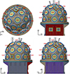 |
Fig. 1. Structural layout of the GECAM payload shown from different perspectives and comprising 25 GRDs (designated G01 through G25) and eight CPDs (designated C01 through C08). The payload comprises two main components: the detector dome housing and the EBOX. The payload coordinate system is defined such that the +X, +Y, and +Z axes align with the central normals of detectors G18, G24, and G01, respectively (Zhao et al. 2023c). |
The GECAM detectors operate in two observational modes: normal mode and South Atlantic Anomaly (SAA) mode. In the normal mode, the detectors record event-by-event, with GRDs and CPDs recording the energy and arrival time of each incident event in real time. When the GRD count rate within several predefined time and energy windows significantly exceeds the background fluctuation, the payload automatically initiates an onboard real-time analysis routine to determine the event’s trigger time, location, classification, and intensity, and promptly downlinks this information to the ground station via the BeiDou satellite navigation system. Upon entering the SAA, the local charged-particle flux rapidly increases, causing a substantial rise in the data volume if keeping record of event-by-event data. Therefore, the payload is set to automatically switch to SAA mode, in which only a few detectors are kept on and the event-by-event data output is turned off. This SAA mode can not only control the data volume but also protect the detectors.
The GECAM satellite operates in two pointing modes: zenith and non-zenith observation. In the normal mode, the satellite conducts continuous all-sky monitoring, with attitude adjustments made according to the observation plan. We define the angle θ between the payload boresight (+Z axis) and the direction toward Earth’s center (0° ≤θ ≤ 180°) to quantify observation attitude. The payload attitude can be adjusted from zenith pointing to non-zenith pointing, as shown in Fig. 2. The observation mode is determined by the preset observation plan.
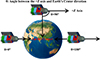 |
Fig. 2. Attitude variations of GECAM during its monitoring mission are shown. The angle θ denotes the angle between the payload coordinate system’s +Z axis and the vector toward the Earth’s center. At θ = 0°, GECAM observes toward the Earth. At θ = 180°, GECAM observes directly away from the Earth. |
There are two pointing modes for GECAM. In the zenith-pointing mode, the boresight of the detector dome points toward the zenith, thus minimizing Earth occultation of the detectors’ field of view (FOV). Data in this mode can be used to investigate how geomagnetic latitude modulates STEs. In the non-zenith pointing mode, the boresight points to directions other than the zenith. By varying the satellite attitude from Earth-pointing to zenith pointing, we can test whether STEs exhibit directional dependence, thereby determining whether they are sourced from specific sky directions. In order to comprehensively investigate the source characteristics of STEs, it is necessary to classify observational data according to satellite pointing mode.
2.2. Data
GECAM data products follow a tiered classification in accordance with standard space astronomy conventions (Zheng et al. 2024b). Remarkably, dedicated scientific data products have been designed and produced for STEs. STE data products are divided into hourly segments. Each file covers a 100 s time window corresponding to the final 100 s of the preceding hour, recording detailed count information from any two or more of the 33 detectors that got events recorded simultaneously, thereby providing basic and convenient data for the temporal and spectral analysis of these STEs.
Due to power constraints on GECAM-A observations, this study only utilizes the event-by-event data (EVT data) by GECAM-B (Cai et al. 2025). The dataset spans multiple orbital periods and covers a wide range of geomagnetic latitudes. To avoid spatial non-uniformity effects of the CPD detectors on the GECAM dome, we analyze only trigger data from 25 GRDs.
The definition of STEs is illustrated in Fig. 3. The time window Δt to identify STEs is defined as 0.3 μs. A STE occurs when at least two detectors register events within this interval. This time window was determined through ground calibration with a 22Na source and on-orbit secondary cosmic-ray measurements to ensure that physically related events (e.g., Compton scattering events, cosmic-ray shower events) could be accurately identified considering the fluctuation in the timing system among GECAM detectors. The choice of Δt = 0.3 μs is further supported by in-orbit timing calibration based on cosmic-ray–induced multi-detector events. Using a one-hour dataset (2022-10-06 06:00:00–06:59:59 UTC) containing 13 353 candidate cosmic-ray events, we find that 97% of the events exhibit a maximum inter-detector trigger-time spread smaller than 0.3 μs, and about 76% have spreads below 0.1 μs. This corresponds to a relative timing precision of approximately 0.1 μs (1σ). A month-by-month stability check covering the period from 2022 August to 2023 July shows no measurable degradation of this timing precision. The absolute timing was independently cross-checked using the Crab pulsar pulse profile, in comparison with Fermi/GBM and GECAM-B, yielding offsets at the level of a few microseconds. Consequently, adopting Δt = 0.3 μs (approximately 3σ) preserves the vast majority of true coincident events while keeping the rate of accidental coincidences negligible (Xiao et al. 2022).
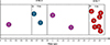 |
Fig. 3. Schematic diagram illustrating STEs. Within a 2 μs interval, two-detector and seven-detector STEs were detected in time windows (a) and (b), respectively. Outside these windows, no events satisfy the simultaneity criterion. Colored spheres indicate the triggered GRDs and their identifiers. |
For each STE event, the number of triggered detectors, N, ranges from 2 to 25 (the total number of GRDs on board). For simplicity, STEs with N triggered detectors are called N-fold STEs or simply referred to as STEs-N throughout this paper. Analysis of the observed data reveals a large number of STEs within a single hour, as shown in Fig. 4.
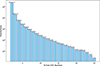 |
Fig. 4. Statistical distribution of STEs observed on-orbit by GECAM-B. The figure illustrates the average number of STEs per hour for varying numbers of detectors triggered (N), depicting the observational characteristics of events that simultaneously trigger multiple detectors. |
3. Coincidence effect on STEs
We note that almost all STEs are expected to correspond to real physical events that leave simultaneous signals in multiple detectors, such as the cosmic-ray showers and Compton scattering, since the probability of multiple detectors being triggered within such a narrow window (0.3 μs) by purely random detector background is vanishingly small. Here we employ GECAM’s on-orbit background count rates and Poisson statistics to demonstrate this.
To verify the physical origin, we denote the mean count rate of the ith detector in time bin j as λi, j in the theoretical calculation. Within a window of width Δt = 0.3 μs, the probability that a single detector triggers at least once is given by
 (1)
(1)
Treating Xi, j ∼ Bernoulli(pi, j) as independent random variables, the number of detectors simultaneously triggered
 (2)
(2)
following a Poisson–binomial distribution. Equivalently,
 (3)
(3)
Recursive convolution is used to extract the polynomial coefficients efficiently. Averaging Pj(K = k) over all time bins yields  . In the Monte Carlo simulation, for each time bin j and detector i, we sample
 (4)
(4)
If ni, j > 0, the detector is considered triggered (i.e., record a signal). Repeating this procedure over all time bins and averaging gives  . Under the assumption of independent detector counts following Poisson processes, the Poisson–binomial model provides theoretical predictions for the N-fold random-coincidence rate. Monte Carlo simulations furnish numerical confirmation of these predictions. The results show that the probability of ≥5 detectors triggering within 0.3 μs due to random counts is extremely low (e.g., 2.24 × 10⁻¹⁴ for N = 5). The theoretical predictions are displayed in Fig. 5. Because Monte Carlo sampling is inherently inefficient for extremely low-probability events, even after hundreds of millions of trials only the k = 2 and k = 3 orders yield nonzero, statistically significant random-coincidence probabilities, whereas for k ≥ 4 virtually no events are sampled. Although such events are exceedingly rare, they are nonetheless observed in the GECAM data.
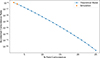 |
Fig. 5. Multi-detector random coincidence probability theoretical calculations (blue circles) and simulation results (orange squares) within a 0.3 μs time window. |
Figure 6 plots the expected random-coincidence probability within one hour as a function of N, and comparison shows that the on-orbit measurements in Fig. 4 lie well above the predicted random-coincidence background. For N = 5, a random coincidence occurs only once every six months on average, implying that STEs with N ≥ 5 cannot be attributed to chance and must share a common physical source. By contrast, during bright gamma-ray episodes, STE-2 can include a physically distinct subpopulation (residual Compton scattering across two detectors after random-coincidence subtraction). More generally, when N ≲ 4, the sample may represent a mixed population in which residual Compton-scattering events and low-multiplicity random coincidences introduce ambiguity into the physical interpretation, whereas for N ≳ 5, the cascade origin becomes dominant and the sample is comparatively clean. For consistency and to ensure sample purity, STEs-2/3/4 are therefore not used to constrain the origin inference in this work, instead, we focus on STEs with N ≥ 5. Notably, both GRDs and CPDs employ fully independent signal-acquisition architectures (Liu et al. 2022). Signals are routed through independent channels into the payload EBOX. The EBOX unifies data acquisition, processing, and transmission and provides bias-voltage regulation for gain control, thus precluding physical crosstalk (Li et al. 2021).
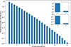 |
Fig. 6. Comparison plot of the expected random coincidence probability versus the number of triggered detectors (N) within one hour. The inset shows an enlarged view of the random coincidence probabilities for N = 2, 3, 4, 5. |
To further investigate the composition of the GECAM-recorded STEs, we take STE-5 as an illustrative example. Several possibilities merit discussion; for instance, four detectors may be genuinely triggered by a single physical particle while an unrelated accidental hit falls within the same 0.3 μs window. Using Bayesian inference, we calculate the posterior probability of having k accidental triggers among the observed five simultaneous triggers, based on the accidental trigger probabilities in each time bin and the prior distribution of the number of genuine triggers. The calculated conditional probabilities of accidental contamination among the observed STEs-5 are 4.30 × 10⁻³ for exactly one accidental hit, 9.82 × 10⁻⁶ for two, 1.59 × 10⁻⁸ for three, and 2.05 × 10⁻¹¹ for four, indicating that STEs-5 are overwhelmingly pure with negligible accidental coincidence events from background.
4. Zenith pointing observation mode
4.1. Correlation with geomagnetic latitude
To investigate the spatial distribution of STEs, we performed systematic analyses using both geographic and geomagnetic latitude as classification parameters. Statistics based on geographic latitude exhibit no obvious spatial pattern, indicating that the conventional geographic coordinate system does not effectively reveal features in STE distribution. When data are categorized by geomagnetic latitude, however, a clear correlation emerges. We converted geographic coordinates to geomagnetic coordinates using the standard Altitude-Adjusted Corrected Geomagnetic Coordinates (AACGM) model (Shepherd 2014) and examined, in geomagnetic latitude, the distribution of the subsatellite point trajectories of STEs detected by GECAM-B during on-orbit operations. To visualize the geomagnetic coverage of STEs, Fig. 7 displays a single continuous UTC day (excluding the SAA region) of STE-5 subsatellite locations, where the one-second binned scatter points appear quasi-continuous along the orbital tracks due to the very high occurrence rate of STEs-5 (cf. Fig. 4). In the equatorial region, the thick black curve denotes the projection of the 0°–15° geomagnetic-latitude band at the satellite’s altitude, where multiple orbital passes overlap. The geomagnetic axis is inclined by approximately 10° relative to the Earth’s rotation axis (Macmillan & Finlay 2010). As a result, the geomagnetic equator is displaced from the geographic equator and exhibits slight undulations with longitude. Consequently, points on the geographic equator map to roughly 0°–15° geomagnetic latitude during the transformation. Based on these geometric features, in the subsequent geomagnetic-latitude classification we selected on-orbit data within the ±400° range, excluding data within the ±15° band, for statistical analysis.
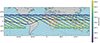 |
Fig. 7. One-day distribution map of subsatellite point trajectories of GECAM-B STEs-5 detected during on-orbit operation, overlaid with geomagnetic latitude. Lines represent the dense one-second scatter along the orbital tracks (excluding the SAA region), colors indicate orbital altitude, and dashed black lines denote geomagnetic latitude contours. |
The geomagnetic modulation of STEs becomes evident through their latitude-dependent energy spectra and integral fluxes. Energy-deposition spectra for STE-5, STE-6, and STE-7 were computed in 5°-wide geomagnetic-latitude bins, as displayed in Fig. 8. Spectra from magnetically symmetric intervals (e.g., [−40°, −36°] vs. [36°, 40°]) display highly consistent shapes, directly reflecting the north–south symmetry of Earth’s magnetic field and its modulation of cosmic-ray transport. Using the spectrum in the [16°, 20°] bin as a reference, we normalize its probability-density function to zero and apply the same normalization to all other bins to extract spectral “shape” parameters. The invariance of these shape parameters across geomagnetic latitudes indicates that the geomagnetic field primarily modulates the occurrence rate of STEs, rather than altering their intrinsic energy-distribution characteristics. The integral flux of STE-5, STE-6, and STE-7 increases monotonically with absolute geomagnetic latitude, as presented in Fig. 9. We note that this latitude-dependent enhancement is consistent with the geomagnetic-rigidity cutoff effect. According to the magnetospheric transmission-function theory (Bobik et al. 2006), cutoff rigidity decreases with increasing geomagnetic latitude, permitting more low-energy cosmic rays to penetrate Earth’s magnetic shielding and reach satellite altitude, thereby boosting the observed primary cosmic-ray flux at high latitudes. This modulation arises because only particles with momentum above the local cutoff rigidity can overcome the Lorentz force exerted by the geomagnetic field. We note that, although the integral flux varies with latitude, the spectral shape remains stable, with differences confined to overall intensity and maximum energy, confirming that the geomagnetic field affects the event rate but not the fundamental physics of STEs.
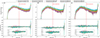 |
Fig. 8. Energy deposition spectra for the STEs at different geomagnetic latitudes. Panels (a), (b), and (c) correspond to STEs-5, STEs-6, and STEs-7, respectively. Upper panels: Energy deposition spectra of STEs at ten different geomagnetic latitudes. Lower panels: Spectral shape differences. The dashed red line indicates the energy value at 511 keV. |
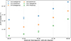 |
Fig. 9. Integrated flux distribution of STEs across different geomagnetic latitude intervals. Blue, orange, and light green correspond to the STE-5, STE-6, and STE-7 configurations, respectively. |
The energy spectra of STEs exhibit a pronounced 511 keV positron-annihilation line (Siegert et al. 2016; Guo et al. 2020). This feature could arise from multiple processes: primary cosmic rays interacting with detector materials produce secondary particles and radioactive isotopes; β+ decay of these isotopes emits positrons that annihilate with electrons in the detector or nearby material, yielding back-to-back γ-ray pairs at 511 keV; and high-energy γ rays (E > 1.022 MeV) generated by cosmic-ray interactions produce electron-positron pairs, whose subsequent annihilation further enhances the 511 keV line (Diehl et al. 2018).
4.2. Detector-geomagnetic field line angular correlation
To further investigate the correlation between STEs and geomagnetic field modulation, we established a quantitative analysis model relating the detector trigger rate to the angle between the detector’s normal vector and the geomagnetic field lines. In this analysis, we compute the angle between the detector’s normal vector and the Earth’s magnetic field lines to quantitatively assess how their relative geometry influences the detector trigger rate. Taking STE-5 as an example, we examined the trigger rate distribution across the GRD array under different geomagnetic latitude conditions. The two-dimensional spatial distribution of GRDs on board the GECAM-B satellite and their corresponding trigger rates at various geomagnetic latitude intervals are presented in Fig. 10. The statistical analysis indicates that the outermost ring detectors (G18–G25) exhibit relatively low trigger rates across all geomagnetic latitudes, a phenomenon attributable to the spatial geometric configuration of the detector array. As edge elements, the outer ring detectors have significantly fewer spatial couplings with adjacent detectors compared to inner ring detectors, resulting in a reduced probability of receiving correlated signals. Considering this geometric effect, data from the outer ring detectors were excluded from the subsequent field-line–direction dependence analysis, in order to minimize spatial-location bias in the study of the physical mechanism.
 |
Fig. 10. Schematic diagram of the two-dimensional spatial distribution of the 25 GRDs (G01–G25) and their trigger rates at different geomagnetic latitudes. The numerical values (%) displayed within each detector denote its average trigger rate, with darker shades indicating higher rates; see the color bar at right for the exact scale. |
The analysis reveals a pronounced negative correlation between the detector trigger rate and the angle relative to the geomagnetic field lines, as illustrated in Fig. 11. When the detector’s normal direction is nearly parallel to the field-line direction (small angle), the trigger rate of STEs is higher; conversely, when they are nearly perpendicular or opposite (large angle), the trigger rate significantly decreases. While the anticorrelation between the GRD trigger rate and the angle to the local geomagnetic field is statistically significant, we caution that GeV galactic cosmic rays at LEO are not magnetically guided along the local field lines. Instead, the geomagnetic field primarily controls the accessibility of charged primaries through the rigidity cutoff and direction-dependent magnetospheric transmission. In this sense, the local field orientation can serve as a convenient proxy for the anisotropy of the allowed arrival directions at a given location. Combined with the geometry-dependent effective acceptance and asymmetric shielding of the payload (dome + EBOX), this naturally produces a correlation between trigger rate and the local field orientation. We therefore interpret the observed correlation as an acceptance/shielding + geomagnetic-transmission effect, rather than magnetic guiding of the secondary cascades.
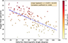 |
Fig. 11. Relationship between detector trigger rates and magnetic field line orientation. The x-axis represents the angle between GRDs and magnetic field lines, while the y-axis represents the GRD trigger rates. The blue line shows the least-squares fit, with the fitting function and correlation coefficient displayed in the upper right corner (where r denotes the strength of the linear relationship between the two variables). |
4.3. Clustering of triggered detectors
To further analyze the physical characteristics of STEs, we examined the spatial distribution of triggered detectors of each STE event. If STEs were produced by independent random particle excitations, the triggered detectors would be expected to exhibit an uncorrelated, random spatial distribution. In this work, we therefore use STE-5 as the analysis sample and define a quantitative clustering index based on pairwise spherical angular separations among the five simultaneously responding detectors.
Let each GRD d have a fixed boresight (θd, ϕd) in the payload frame (polar and azimuthal angles), and define the associated unit vector
 (5)
(5)
For a given STE with detector set S = {d1, …, dm}, the spherical pairwise angular separation between detectors i and j is defined as
 (6)
(6)
We summarize the spatial configuration by the following statistics over all unordered pairs i < j:
 (7)
(7)
We adopt  as the primary clustering index (smaller values indicate tighter spatial clustering), which provides a compact numerical descriptor of each event’s detector geometry and effectively characterizes the degree of clustering or dispersion within a detector combination.
To test against the null hypothesis that STEs arise from random, uncorrelated triggers, we generate a null distribution of  via Monte Carlo by drawing m-tuples (without replacement) from the 25 GRDs, with m = 5 to match the STE-5 sample. We then compare the observed and null distributions (Fig. 12) using the two-sided Mann–Whitney U test (Hill et al. 2018), which assesses whether the central tendencies (location parameters) of two independent samples are consistent with being drawn from the same parent distribution. We report the test p-value together with an effect size
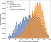 |
Fig. 12. Distribution of clustering characteristics for STE-5. The histogram for on-orbit data is compared with (i) randomly simulated triggers (null hypothesis) and (ii) an end-to-end Monte Carlo (MC) simulation based on the full spacecraft mass model of GECAM-B, with isotropic primary protons and α particles. The MC result reproduces the observed mean-angular-distance distribution, indicating that the measured clustering is compatible with cascade footprints in the spacecraft structures. |
 (8)
(8)
The resulting p-value is extremely small, indicating that the observed events are not consistent with the random model. The mean clustering index of the on-orbit events (Orbit Mean) deviates markedly from the theoretical expectation for simulated combinations (Simulation Mean), quantitatively confirming pronounced spatial clustering among simultaneously triggered detectors.
Physically, STEs preferentially involve detectors that are spatially adjacent, whereas combinations spanning large angular separations are comparatively rare. This pattern is naturally explained if STEs originate from particle showers: high-energy cosmic-ray primaries impinging on the spacecraft structure generate cascades of secondary particles in the surrounding materials, which then trigger multiple neighboring detectors within the 0.3 μs window. The observed clustering, together with the statistical rejection of the random-hypothesis model, provides direct empirical support for a cosmic-ray–induced cascade origin of STEs.
To directly compare the observed clustering with physically motivated cascade footprints, we performed an end-to-end Monte Carlo simulation using the full spacecraft mass model of GECAM-B, injecting isotropic primary protons and α particles in the 0.5 GeV–1 TeV range. For simulated events passing the STE-5 selection, we compute the same clustering indices as for the data. The resulting mean-angular-distance distribution (labeled “MC” in Fig. 12) closely reproduces the on-orbit distribution, whereas the purely random simulation does not. This agreement supports the interpretation that the spatial clustering of STEs is consistent with secondary-particle cascades developing in the spacecraft structures.
5. Non-zenith pointing observation mode
Based on observations of how STEs depend on magnetic field orientation, this section investigates the characteristics of their spatial origin, with particular emphasis on determining whether they originate from external signals coming from specific directions in the sky or from the Earth. The analysis employs a comparative approach under different satellite-pointing conditions, examining the patterns of variation in energy-deposition spectra and integrated fluxes. As mentioned above, we use the angle between the satellite’s Z-axis and the geocenter, denoted θ, which ranges from 0° (Z-axis pointing directly toward the geocenter) to 180° (Z-axis pointing directly away toward deep space). To eliminate systematic interference arising from variations in geomagnetic latitude, only observations collected at a fixed geomagnetic latitude are selected for this study. A sample of STEs-5 is selected for analysis. Four representative angular intervals are defined: 4° −15°, 59° −81°, 125° −143°, and 165° −175°. These intervals cover the full range of satellite attitudes, from Earth-pointing to nearly zenith-pointing.
The statistical analysis reveals that the energy deposition spectra for STEs maintain highly consistent shapes across all four angular intervals, with no systematic shifts observed in the relative intensity distributions across energy bands, as shown in Fig. 13. We note, however, an apparent line feature around ∼6–7 MeV, which is an instrumental artifact: above ∼5 MeV, STEs induce saturation effects in the GRDs, leading to line-like structures in the count spectra. Therefore, all quantitative comparisons of spectral shapes in this section are confined to the non-saturated energy range (20 keV–5 MeV), and events affected by overflow are excluded to prevent biases introduced by detector saturation. Furthermore, the integrated fluxes of STEs remain essentially constant across these angular intervals, as shown in Fig. 14. The detector trigger rates at different pointing angles (as shown in Fig. 15) and their correlation with magnetic field-line inclination angles (as shown in Fig. 16) provide additional insights into the nature of these events. The study finds a significant negative correlation between detector trigger rates and field-line inclination angles at all pointing angles. Notably, under fixed geomagnetic latitude conditions, the non-zenith pointing mode exhibits a stronger negative correlation than the zenith pointing mode. The absolute value of the correlation coefficient is markedly increased. This difference can be attributed to the modulation effect of geomagnetic latitude. By fixing the geomagnetic latitude, gradients of magnetic field strength with latitude are eliminated. Consequently, the influence of field-line inclination angle can be isolated more cleanly, enhancing the statistical significance of the correlation. The energy spectrum shapes and integrated fluxes of STEs remain stable across all satellite attitudes. No systematic response patterns are observed in relation to attitude changes. This stability effectively excludes the possibility that the STEs have their source in external signals fixed in a particular sky direction. If they did, changes in satellite pointing would produce corresponding variations in event rates or spectral shapes. The observed consistency suggests that these STEs are more likely to exhibit isotropic distributions or arise from physical processes within the local satellite environment.
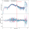 |
Fig. 13. Energy deposition spectra of STEs at different pointing angles under the same geomagnetic latitude, with the dashed red line corresponding to the energy value at 511 keV. |
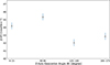 |
Fig. 14. Integrated flux of STEs at different pointing angles under the same geomagnetic latitude. |
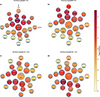 |
Fig. 15. Schematic diagram of GRD trigger rates at different pointing angles under the same geomagnetic latitude. |
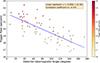 |
Fig. 16. Relationship between GRD trigger rates and magnetic field line directions at the same geomagnetic latitude. |
6. Energy spectrum analysis
To further elucidate the physical nature of STEs, we compare the energy-deposition spectra of single-detector background events with those of STEs for multiplicities N = 5, 10, 20, 25. The brown curve in Fig. 17 represents the spectrum of events triggering only one detector within a 0.3 μs time window (right-hand vertical axis). In the single-detector spectrum, a delayed background peak appears around 410 keV, arising from the decay of radioactive nuclides activated in spacecraft materials. Since decay is a stochastic process whose timing depends on the nuclides’ half-lives and thus occurs with a characteristic lag, this component is termed the delayed background (Guo et al. 2020). An intrinsic background peak at 1470 keV is attributed to 138La decay in LaBr3 scintillators (Zhang et al. 2019; Quarati et al. 2012), and the 511 keV feature corresponds to positron annihilation radiation induced by space radiation particles. By contrast, the spectra of STEs (red, green, blue, and magenta curves in Fig. 17 for N = 5, 10, 20, 25, respectively) effectively suppress both intrinsic and delayed background contributions, confirming that the coincidence-trigger mechanism selects non-background physical events. The similarity of these spectra across different N values indicates a common physical source, while the increasing statistical uncertainty with higher N reflects the rarity of high-multiplicity events. Using the N = 5 spectrum as a reference, we shift its probability-density function to a zero baseline and apply the same procedure to the other spectra in order to extract their “shape” characteristics. Analysis of the spectral-shape evolution reveals a dual trend bifurcated at 511 keV: photon counts in the low-energy region (20 keV − 511 keV) decrease with increasing N, whereas counts in the high-energy region (511 keV − 5 MeV;non-saturated) increase. Events flagged as overflow (energy deposition above the low-gain calibration range) are excluded from the spectral-shape analysis; we verified that the reported spectral evolution with N remains unchanged after removing all overflow events, indicating that the low-energy suppression and high-energy enhancement are not artifacts of saturation. The 511 keV annihilation peak persists across all multiplicities but diminishes in relative intensity as N grows, likely because high-N cosmic-ray events induce more extensive secondary particle cascades in the detector array, amplifying high-energy counts and diluting the annihilation feature.
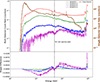 |
Fig. 17. Schematic diagram showing the evolution of single detector event spectra and STE spectra. The brown line represents the single detector event spectrum, corresponding to the right-hand vertical axis. From left to right, the two brown arrows indicate delayed background and intrinsic background, respectively. The red, green, blue, and magenta spectral lines correspond to STEs involving 5, 10, 20, and 25 detectors, respectively. Lower panel: Spectral-shape variations of STEs involving 10, 20, and 25 detectors, using the STE-5 spectrum as the reference baseline. |
Overall, as N increases from 5 to 25, the spectral centroid shifts progressively toward higher energies. This evolution aligns with the energy-deposition processes of cosmic rays in detector materials: higher multiplicities correspond to incident particles of greater energy, more complex secondary cascades, larger numbers of triggered detectors, and greater total deposited energy. The observed dual-evolution pattern can be ascribed to energy-threshold effects in cosmic-ray interactions: low-energy cosmic rays deposit energy chiefly via ionization losses in one or a few detectors, producing limited secondary particles and low-multiplicity triggers; high-energy cosmic rays have sufficient energy to initiate nuclear interactions, generating abundant secondary particles (neutrons, protons, mesons, etc.) that form extensive showers across the array and trigger multiple detectors simultaneously (Grieder 2001). The ubiquitous presence of the 511 keV annihilation peak underscores positron production as a hallmark of high-energy cosmic-ray interactions, and its dependence on N reflects the intrinsic link between cascade development and incident-particle energy.
7. Possible origin of STEs
In this section we discuss the potential production mechanism of STEs. We primarily evaluate two likely scenarios involving high-energy cosmic rays: the atmospheric scenario and the satellite scenario.
In the atmospheric-origin scenario, STEs are hypothesized to arise from secondary particles produced when high-energy cosmic rays interact with Earth’s atmosphere, primarily with oxygen and nitrogen nuclei (Ren et al. 2024). A fraction of these secondary particles may be backscattered into space and subsequently detected by GECAM. However, our observations are inconsistent with this hypothesis in several key aspects.
First, if STEs were predominantly of atmospheric origin, GECAM would be expected to record substantially stronger signals during Earth-pointing observations and significantly weaker signals when pointing toward the zenith. In contrast, both the energy spectra and occurrence rates of STEs are found to be essentially invariant across all spacecraft pointing attitudes. Second, previous measurements (Alcaraz et al. 2000), together with earlier studies of atmospheric albedo, have shown that the flux of upward-going (albedo) charged particles peaks near the geomagnetic equator and decreases toward higher geomagnetic latitudes. This behavior is incompatible with our observation that the STE flux increases with geomagnetic latitude. Third, published albedo studies indicate that at an altitude of approximately 600 km, the upward fluxes of neutrons and gamma rays in the energy range from tens of MeV to GeV are extremely low and decrease further with increasing energy. The upward neutron energy spectrum has been reported as (Armstrong et al. 1973; Morris et al. 1998)
 (9)
(9)
and the corresponding upward gamma-ray spectrum as (Mizuno et al. 2004; Abdo et al. 2009)
 (10)
(10)
where the units are cm−2 s−1 MeV−1. Rapid Monte Carlo estimates based on these representative upward spectra demonstrate that the contribution of such neutral secondary particles to STEs with multiplicity N ≥ 5 within a sub-microsecond coincidence window is negligible. Upward-going muons are also unlikely to constitute a significant component at an altitude of 600 km, owing to their finite lifetime and decay length. Only muons with energies ≳100 GeV could survive to such altitudes, but their upward flux is expected to be vanishingly small (Garg et al. 2025). Finally, the coincidence time scale itself further disfavors an atmospheric origin. Producing N ≥ 5 nearly simultaneous triggers within Δt = 0.3 μs in a compact detector array would require an atmospheric shower at orbital altitude with an exceptionally rare geometric configuration. While so-called “grazing atmospheric showers” have been discussed in the literature (Ulmer 1994), they are typically associated with much longer, millisecond-scale temporal signatures. We note that extreme edge cases – for example, ultra-high-energy primaries producing very grazing showers that skim the atmosphere and intercept the spacecraft at orbital altitude – are not strictly impossible in principle; however, their expected flux and the geometry- and timing-constrained probability of generating N ≥ 5 coincident events within Δt = 0.3 μs are so small that they can be regarded as theoretical curiosities with negligible practical contribution. Taken together, these considerations indicate that atmospheric secondary particles are unlikely to be the dominant source of STEs.
In the satellite scenario, STEs originate directly from cosmic-ray interactions in the satellite detectors or nearby materials. Incident cosmic-ray particles strike spacecraft materials and initiate secondary-particle cascades–comprising ionization products and high-energy photons–that emit quasi-isotropically and are recorded nearly simultaneously by multiple detectors. Primary cosmic rays are charged, so their trajectories are modulated by the geomagnetic rigidity cutoff. At high latitudes, a lower cutoff permits more high-energy cosmic rays to reach the satellite. The spatial clustering of simultaneously triggered detectors on the satellite platform aligns with the geometry of cascade propagation in the spacecraft material. Moreover, as detector multiplicity N increases, the energy spectrum evolves from being dominated by low-energy particles to being dominated by high-energy particles. The persistent 511 keV annihilation peak reflects the production of positrons in these cascades. Both features are in full agreement with high-energy particle cascade physics. The satellite scenario also accounts for the independence of STE characteristics from satellite pointing. Although Earth should block primary cosmic rays over an approximate 2π sr solid angle when Earth-pointing, the measured energy spectra and integrated fluxes remain statistically unchanged for all attitudes. This pointing-independence indicates that STEs are not tied to any specific incident direction of primary cosmic rays. Instead, they are governed by secondary cascades within spacecraft materials. Even if Earth occludes certain directions, cosmic rays from unobstructed directions still produce similar cascades, maintaining the statistical stability of STE properties. Taken together, the satellite scenario self-consistently explains all observed features, whereas the atmospheric scenario exhibits multiple contradictions. We therefore conclude that STEs are primarily sourced from direct interactions of cosmic rays with the satellite detectors and their surrounding materials.
Following the exclusion of atmospheric-origin scenarios based on observational constraints, we further investigate whether STEs can be quantitatively explained as particle cascades induced by cosmic rays interacting with the spacecraft itself. To this end, we carried out end-to-end Monte Carlo simulations using the full GEANT4 mass model of GECAM-B. Primary protons and α particles were injected isotropically with energies spanning from 0.5 GeV to 1 TeV. Figure 18 summarizes the normalized event yields producing different STE multiplicity intervals (2–5, 6–10, 11–15, 16–20, and 21–25) as functions of the primary particle energy. As the STE multiplicity interval increases, both the onset (minimum) primary energy and the energy band at which the yield peaks shift systematically toward higher energies, while the overall normalized yield decreases. This trend indicates that higher-multiplicity STEs require increasingly energetic primary particles and are intrinsically rarer. Although the absolute normalization of the simulated yields may be affected by uncertainties in the incident cosmic-ray spectra and by residual simplifications in the detector response(e.g., the lack of a full electronics chain such as SiPM/electronics nonlinearities or saturation, threshold/pile-up effects, and dead-time coupling), the full mass model accurately captures the global material distribution and geometric configuration of the spacecraft. Consequently, the relative trends with primary energy and STE multiplicity are robust, whereas the absolute rate normalization is the quantity most sensitive to these unmodeled effects. Taken together, these results provide direct, model-based support for interpreting STEs as cascades generated locally by cosmic rays interacting with spacecraft structures, rather than as products of atmospheric secondary particles.
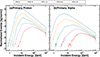 |
Fig. 18. Normalized event yields of simulated STEs as a function of primary particle energy for different multiplicity intervals (2–5, 6–10, 11–15, 16–20, and 21–25), obtained from end-to-end GEANT4 simulations using the full mass model of GECAM-B. |
8. Discussion and summary
In this study, we performed the first systematic analysis of the STEs detected by the all-sky gamma-ray monitor and explored the possible origin of these interesting events. We find that these STEs detected by GECAM-B exhibit clear characteristics of a true physical event, rather than instrumental noise or random coincidence. The count rate of STEs increases as geomagnetic latitude increases, which is consistent with the cosmic-ray rigidity cutoff effect. The observed spatial clustering of triggered detectors on the STE satellite, confirmed by MC simulations, further supports this interpretation. We confirm a statistically significant correlation between STE rates and the local geomagnetic-field orientation. We interpret this correlation as a geomagnetic-transmission (rigidity cutoff and direction-dependent access) effect convolved with the geometry- and shielding-dependent effective acceptance of the payload, rather than magnetic guiding of secondary cascades. Under different satellite pointing modes (i.e., zenith and non-zenith), the deposited energy spectrum of STEs remains stable, which rules out any source in a particular sky region. As the number of simultaneously triggered detectors (N) increases, the spectral centroid shifts toward higher energies, and a pronounced 511 keV annihilation peak becomes apparent. Moreover, the spectral evolution of STEs aligns with the cosmic-ray–induced cascade scenario. These results support the scenario that the primary source of STEs is the cascade of secondary particles produced by high-energy cosmic rays interacting with the satellite, and the contribution from atmospheric secondary particles is not the dominant component.
We note that this finding carries important implications. First, STEs may be misclassified as transient high-energy phenomena such as terrestrial gamma-ray flashes (Fishman et al. 1994; Dwyer et al. 2012; Yi et al. 2025); our analysis provides a criterion to discriminate such false triggers by STEs. Second, STEs exhibit a well-defined physical source and high synchronicity, making them very suitable for the in-flight calibration of relative timing resolution among detectors in a multi-detector system.
We stress that GECAM was not initially designed to detect and study cosmic rays, and this is a by-product of the special design of the GECAM instrument. For other GECAM-like all-sky monitors, cosmic-ray–induced multi-detector coincident triggers were typically regarded as background noise and directly filtered out. Although this approach enhances the signal-to-noise ratio for the targeted astrophysical events, it sacrifices the valuable physical information carried by the cosmic rays. Taking advantage of the sub-microsecond time resolution (0.1 μs) of detectors, GECAM can record and identify STEs and thus use them as a qualitative and semi-quantitative diagnostic of the near-earth high-energy cosmic-ray environment. Because STEs are produced by secondary cascades in spacecraft materials, GECAM may not be a precision cosmic-ray spectrometer, and any inference of primary energy or composition is indirect and model-dependent.
In summary, this work has not only systematically characterized the observational features of STEs detected by GECAM, but also discussed the high-energy cosmic-ray origin of these STEs, deepening our understanding of near-Earth high-energy cosmic-ray particle environments and their interactions with satellites. To further constrain the properties (such as the particle type and energy) of high-energy cosmic rays from STEs, more work needs to be done, including (i) developing a GEANT4-based end-to-end model of the spacecraft–detector system to establish the quantitative relationship between the properties of incident particles (including their energy and composition) and the spectral evolution (STE-N) distribution. Because the detector primarily records secondary products generated in the cascade process initiated by the incident particles rather than the primary particles themselves, the model will incorporate the effects of spacecraft geometry, material composition, and limitations arising from detector readout nonlinearity as well as dead-time and pile-up or threshold effects; it will also (ii) analyze STE-2/3/4 data to disentangle Compton scattering from particle cascades under both burst and quiet conditions. These efforts are crucial to achieving the transition from qualitative diagnostics to quantitative reconstruction of cosmic rays (while the present work focuses on robust qualitative and semi-quantitative trends rather than absolute-flux calibration).
Acknowledgments
We thank the anonymous referee for the constructive comments and suggestions that greatly improved this manuscript. This work is supported by the National Natural Science Foundation of China (Grant No. 12273042, 12494572), the National Key R&D Program of China (2022YFF0711404, 2021YFA0718500), the Strategic Priority Research Program of Chinese Academy of Sciences (Grant Nos. XDA15360102, XDA15360300, XDA30050000, XDB0550300), and supported by the fund of the Key Laboratory of Cosmic Rays (Xizang University), Ministry of Education (Grant No. KLCR-2025**). The GECAM (Huairou-1) mission is supported by the Strategic Priority Research Program on Space Science (Grant No. XDA15360000) of the Chinese Academy of Sciences. We thank the development and operation teams of GECAM.
References
- Abbott, B. P., Abbott, R., Abbott, T. D., et al. 2017, ApJ, 848, L13 [CrossRef] [Google Scholar]
- Abdo, A. A., Ackermann, M., Ajello, M., et al. 2009, Phys. Rev. D, 80, 122004 [NASA ADS] [CrossRef] [Google Scholar]
- Agrawal, P. C. 2006, Adv. Space Res., 38, 2989 [Google Scholar]
- Aguilar, M., Aisa, D., Alpat, B., et al. 2015, Phys. Rev. Lett., 114, 171103 [CrossRef] [PubMed] [Google Scholar]
- Alcaraz, J., Alvisi, D., Alpat, B., et al. 2000, Phys. Lett. B, 472, 215 [Google Scholar]
- An, Z. H., Sun, X. L., Zhang, D. L., et al. 2022, Radiat. Detect. Technol. Methods, 6, 43 [Google Scholar]
- Aptekar, R. L., Frederiks, D. D., Golenetskii, S. V., et al. 1995, Space Sci. Rev., 71, 265 [NASA ADS] [CrossRef] [Google Scholar]
- Armstrong, T. W., Chandler, K. C., & Barish, J. 1973, J. Geophys. Res., 78, 2715 [Google Scholar]
- Bernardini, M. G., Ghirlanda, G., Campana, S., et al. 2015, MNRAS, 446, 1129 [Google Scholar]
- Bobik, P., Boella, G., Boschini, M. J., et al. 2006, J. Geophys. Res. (Space Phys.), 111, A05205 [Google Scholar]
- Briggs, M. S., Fishman, G. J., Connaughton, V., et al. 2010, J. Geophys. Res. (Space Phys.), 115, A07323 [Google Scholar]
- Briggs, M. S., Xiong, S., Connaughton, V., et al. 2013, J. Geophys. Res. Space Phys., 118, 3805 [Google Scholar]
- Cai, C., Zhang, Y.-Q., Xiong, S.-L., et al. 2025, Sci. China Phys. Mech. Astron., 68, 239511 [Google Scholar]
- Diehl, R., Siegert, T., Greiner, J., et al. 2018, A&A, 611, A12 [NASA ADS] [CrossRef] [EDP Sciences] [Google Scholar]
- Dwyer, J. R., Smith, D. M., & Cummer, S. A. 2012, Space Sci. Rev., 173, 133 [Google Scholar]
- Feng, P.-Y., & Sun, X.-L. 2024, Nucl. Instrum. Methods Phys. Res. A, 1069, 169826 [Google Scholar]
- Feng, P.-Y., An, Z.-H., Zhang, D.-L., et al. 2024, Sci. China Phys. Mech. Astron., 67, 111013 [Google Scholar]
- Fishman, G. J., Bhat, P. N., Mallozzi, R., et al. 1994, Science, 264, 1313 [Google Scholar]
- Garg, D., Pradip Das, L., & Hall Reno, M. 2025, ArXiv e-prints [arXiv:2510.03428] [Google Scholar]
- Goldstein, A., Veres, P., Burns, E., et al. 2017, ApJ, 848, L14 [CrossRef] [Google Scholar]
- Grieder, P. K. 2001, Cosmic rays at Earth (Elsevier) [Google Scholar]
- Guo, D., Peng, W., Zhu, Y., et al. 2020, Sci. Sin. Phys. Mech. Astron., 50, 129509 [Google Scholar]
- Hill, R., Shariff, H., Trotta, R., et al. 2018, MNRAS, 481, 2766 [Google Scholar]
- Huppenkothen, D., Heil, L. M., Watts, A. L., & Göğüş, E. 2014, ApJ, 795, 114 [Google Scholar]
- Li, T., Xiong, S., Zhang, S., et al. 2018, Sci. China Phys. Mecha. Astron., 61, 031011 [Google Scholar]
- Li, X., Wen, X., Xiong, S., et al. 2025, Exp. Astron., 59, 22 [Google Scholar]
- Li, X. Q., Wen, X. Y., Xiong, S. L., et al. 2021, ArXiv e-prints [arXiv:2112.04772] [Google Scholar]
- Li, X. Q., Wen, X. Y., An, Z. H., et al. 2022, Radiat. Detect. Technol. Methods, 6, 12 [Google Scholar]
- Liu, C., Zhang, Y., Li, X., et al. 2020, Sci. China Phys. Mech. Astron., 63, 249503 [NASA ADS] [CrossRef] [Google Scholar]
- Liu, Y. Q., Gong, K., Li, X. Q., et al. 2022, Radiat. Detect. Technol. Methods, 6, 70 [Google Scholar]
- Luo, X. H., Xiao, S., Zheng, S.-J., et al. 2023, ApJS, 266, 16 [Google Scholar]
- Macmillan, S., & Finlay, C. 2010, Geomagnetic Observations and Models (Springer), 265 [Google Scholar]
- Meegan, C., Lichti, G., Bhat, P. N., et al. 2009, ApJ, 702, 791 [Google Scholar]
- Mizuno, T., Kamae, T., Godfrey, G., et al. 2004, ApJ, 614, 1113 [NASA ADS] [CrossRef] [Google Scholar]
- Moradi, R., Wang, C. W., Zhang, B., et al. 2024, ApJ, 977, 155 [Google Scholar]
- Morris, D. J., Aarts, H., Bennett, K., et al. 1998, Adv. Space Res., 21, 1789 [Google Scholar]
- Quarati, F. G. A., Khodyuk, I. V., van Eijk, C. W. E., Quarati, P., & Dorenbos, P. 2012, Nucl. Instrum. Methods Phys. Res. A, 683, 46 [Google Scholar]
- Ren, Y. Z., Chen, T.-L., Feng, Y.-L., et al. 2024, Res. Astron. Astrophys., 24, 035007 [Google Scholar]
- Roberts, O. J., Baring, M. G., Huppenkothen, D., et al. 2023, ApJ, 956, L27 [Google Scholar]
- Sakamoto, T., Barthelmy, S. D., Barbier, L., et al. 2008, ApJS, 175, 179 [NASA ADS] [CrossRef] [Google Scholar]
- Shepherd, S. 2014, J. Geophys. Res. Space Phys., 119, 7501 [Google Scholar]
- Siegert, T., Diehl, R., Khachatryan, G., et al. 2016, A&A, 586, A84 [NASA ADS] [CrossRef] [EDP Sciences] [Google Scholar]
- Su, Y., Peng, W., Chen, W., et al. 2020, Sci. Sin. Phys. Mech. Astron., 50, 129505 [Google Scholar]
- Ulmer, A. 1994, ApJ, 429, L95 [Google Scholar]
- von Kienlin, A., Beckmann, V., Rau, A., et al. 2003, A&A, 411, L299 [NASA ADS] [CrossRef] [EDP Sciences] [Google Scholar]
- Wang, C., Zhang, Y., Xiong, S., et al. 2024, Chin. J. Space Sci., 44, 668 [Google Scholar]
- Xiao, S., Xiong, S. L., Zhang, S. N., et al. 2021, ApJ, 920, 43 [Google Scholar]
- Xiao, S., Liu, Y. Q., Peng, W. X., et al. 2022, MNRAS, 511, 964 [NASA ADS] [CrossRef] [Google Scholar]
- Xiao, S., Liu, Y.-Q., Gong, K., et al. 2024, ApJS, 270, 3 [NASA ADS] [CrossRef] [Google Scholar]
- Xie, S.-L., Cai, C., Yu, Y.-W., et al. 2025, ApJS, 277, 5 [Google Scholar]
- Xiong, S. 2020, Sci. Sin. Phys. Mech. Astron., 50, 129501 [Google Scholar]
- Xu, Y. B., Li, X. Q., Sun, X. L., et al. 2022, Radiat. Detect. Technol. Methods, 6, 53 [Google Scholar]
- Yadav, J. S., Agrawal, P. C., Antia, H. M., et al. 2017, Curr. Sci., 113, 591 [Google Scholar]
- Yi, Q., Zhao, Y., Xiong, S., et al. 2025, Sci. China Phys. Mech. Astron., 68, 251013 [Google Scholar]
- Zhang, D., Li, X., Xiong, S., et al. 2019, Nucl. Instrum. Methods Phys. Res. A, 921, 8 [Google Scholar]
- Zhang, D. L., Sun, X. L., An, Z. H., et al. 2022a, Radiat. Detect. Technol. Methods, 6, 63 [Google Scholar]
- Zhang, P., Ma, X., Huang, Y., et al. 2022b, Radiat. Detect. Technol. Methods, 6, 3 [Google Scholar]
- Zhang, S. N., Li, T., Lu, F., et al. 2020, Sci. China Phys. Mech. Astron., 63, 249502 [NASA ADS] [CrossRef] [Google Scholar]
- Zhang, Y. Q., Xiong, S.-L., Mao, J.-R., et al. 2024, Sci. China Phys. Mech. Astron., 67, 289511 [Google Scholar]
- Zhao, H. S., Li, D., Xiong, S.-L., et al. 2023a, Sci. China Phys. Mech. Astron., 66, 259611 [NASA ADS] [CrossRef] [Google Scholar]
- Zhao, Y., Liu, J. C., Xiong, S. L., et al. 2023b, Geophys. Res. Lett., 50, e2022GL102325 [Google Scholar]
- Zhao, Y., Xue, W.-C., Xiong, S.-L., et al. 2023c, ApJS, 265, 17 [Google Scholar]
- Zheng, C., An, Z.-H., Peng, W.-X., et al. 2024a, Nucl. Instrum. Methods Phys. Res. A, 1059, 169009 [Google Scholar]
- Zheng, S., Song, L., Ma, X., et al. 2024b, Res. Astron. Astrophys., 24, 104001 [Google Scholar]
- Zheng, S. J., Zhang, S. N., Lu, F. J., et al. 2019, ApJS, 244, 1 [Google Scholar]
They are sometimes called events or triggers.
All Figures
|
Fig. 1. Structural layout of the GECAM payload shown from different perspectives and comprising 25 GRDs (designated G01 through G25) and eight CPDs (designated C01 through C08). The payload comprises two main components: the detector dome housing and the EBOX. The payload coordinate system is defined such that the +X, +Y, and +Z axes align with the central normals of detectors G18, G24, and G01, respectively (Zhao et al. 2023c). |
| In the text | |
|
Fig. 2. Attitude variations of GECAM during its monitoring mission are shown. The angle θ denotes the angle between the payload coordinate system’s +Z axis and the vector toward the Earth’s center. At θ = 0°, GECAM observes toward the Earth. At θ = 180°, GECAM observes directly away from the Earth. |
| In the text | |
|
Fig. 3. Schematic diagram illustrating STEs. Within a 2 μs interval, two-detector and seven-detector STEs were detected in time windows (a) and (b), respectively. Outside these windows, no events satisfy the simultaneity criterion. Colored spheres indicate the triggered GRDs and their identifiers. |
| In the text | |
|
Fig. 4. Statistical distribution of STEs observed on-orbit by GECAM-B. The figure illustrates the average number of STEs per hour for varying numbers of detectors triggered (N), depicting the observational characteristics of events that simultaneously trigger multiple detectors. |
| In the text | |
|
Fig. 5. Multi-detector random coincidence probability theoretical calculations (blue circles) and simulation results (orange squares) within a 0.3 μs time window. |
| In the text | |
|
Fig. 6. Comparison plot of the expected random coincidence probability versus the number of triggered detectors (N) within one hour. The inset shows an enlarged view of the random coincidence probabilities for N = 2, 3, 4, 5. |
| In the text | |
|
Fig. 7. One-day distribution map of subsatellite point trajectories of GECAM-B STEs-5 detected during on-orbit operation, overlaid with geomagnetic latitude. Lines represent the dense one-second scatter along the orbital tracks (excluding the SAA region), colors indicate orbital altitude, and dashed black lines denote geomagnetic latitude contours. |
| In the text | |
|
Fig. 8. Energy deposition spectra for the STEs at different geomagnetic latitudes. Panels (a), (b), and (c) correspond to STEs-5, STEs-6, and STEs-7, respectively. Upper panels: Energy deposition spectra of STEs at ten different geomagnetic latitudes. Lower panels: Spectral shape differences. The dashed red line indicates the energy value at 511 keV. |
| In the text | |
|
Fig. 9. Integrated flux distribution of STEs across different geomagnetic latitude intervals. Blue, orange, and light green correspond to the STE-5, STE-6, and STE-7 configurations, respectively. |
| In the text | |
|
Fig. 10. Schematic diagram of the two-dimensional spatial distribution of the 25 GRDs (G01–G25) and their trigger rates at different geomagnetic latitudes. The numerical values (%) displayed within each detector denote its average trigger rate, with darker shades indicating higher rates; see the color bar at right for the exact scale. |
| In the text | |
|
Fig. 11. Relationship between detector trigger rates and magnetic field line orientation. The x-axis represents the angle between GRDs and magnetic field lines, while the y-axis represents the GRD trigger rates. The blue line shows the least-squares fit, with the fitting function and correlation coefficient displayed in the upper right corner (where r denotes the strength of the linear relationship between the two variables). |
| In the text | |
|
Fig. 12. Distribution of clustering characteristics for STE-5. The histogram for on-orbit data is compared with (i) randomly simulated triggers (null hypothesis) and (ii) an end-to-end Monte Carlo (MC) simulation based on the full spacecraft mass model of GECAM-B, with isotropic primary protons and α particles. The MC result reproduces the observed mean-angular-distance distribution, indicating that the measured clustering is compatible with cascade footprints in the spacecraft structures. |
| In the text | |
|
Fig. 13. Energy deposition spectra of STEs at different pointing angles under the same geomagnetic latitude, with the dashed red line corresponding to the energy value at 511 keV. |
| In the text | |
|
Fig. 14. Integrated flux of STEs at different pointing angles under the same geomagnetic latitude. |
| In the text | |
|
Fig. 15. Schematic diagram of GRD trigger rates at different pointing angles under the same geomagnetic latitude. |
| In the text | |
|
Fig. 16. Relationship between GRD trigger rates and magnetic field line directions at the same geomagnetic latitude. |
| In the text | |
|
Fig. 17. Schematic diagram showing the evolution of single detector event spectra and STE spectra. The brown line represents the single detector event spectrum, corresponding to the right-hand vertical axis. From left to right, the two brown arrows indicate delayed background and intrinsic background, respectively. The red, green, blue, and magenta spectral lines correspond to STEs involving 5, 10, 20, and 25 detectors, respectively. Lower panel: Spectral-shape variations of STEs involving 10, 20, and 25 detectors, using the STE-5 spectrum as the reference baseline. |
| In the text | |
|
Fig. 18. Normalized event yields of simulated STEs as a function of primary particle energy for different multiplicity intervals (2–5, 6–10, 11–15, 16–20, and 21–25), obtained from end-to-end GEANT4 simulations using the full mass model of GECAM-B. |
| In the text | |
Current usage metrics show cumulative count of Article Views (full-text article views including HTML views, PDF and ePub downloads, according to the available data) and Abstracts Views on Vision4Press platform.
Data correspond to usage on the plateform after 2015. The current usage metrics is available 48-96 hours after online publication and is updated daily on week days.
Initial download of the metrics may take a while.