| Issue |
A&A
Volume 707, March 2026
|
|
|---|---|---|
| Article Number | A361 | |
| Number of page(s) | 12 | |
| Section | Planets, planetary systems, and small bodies | |
| DOI | https://doi.org/10.1051/0004-6361/202558471 | |
| Published online | 24 March 2026 | |
The stratification of planetary regolith: Investigating the relation between turnover pressure and grain size
1
Institute of Geophysics and Extraterrestrial Physics (IGEP), Technische Universität Braunschweig,
Mendelssohnstr. 3,
38106
Braunschweig,
Germany
2
Institut für Planetologie (IfP), Universität Münster,
Wilhelm-Klemm-Str. 10,
48149
Münster,
Germany
★ Corresponding author: This email address is being protected from spambots. You need JavaScript enabled to view it.
Received:
8
December
2025
Accepted:
31
January
2026
Abstract
Context. In the gravitational surface field of airless Solar System bodies, regolith should show densification when moving from the surface to greater depths.
Aims. We aim to validate and constrain basic parameters of an existing regolith stratification model by using literature data on the compression of granular media.
Methods. We analysed granular-matter compression curves and determined the turnover pressure from the loose to the compact state and the logarithmic transition width between the two states. In addition, we analysed laboratory measurements of the average packing fraction of granular samples as a function of grain size with respect to the turnover pressure.
Results. We were able to derive the turnover pressure for grain radii between ∼0.5 μm and ∼100 μm. The relation between turnover pressure and particle size follows a power law with slope −2, as suggested by a dust aggregate compression model.
Conclusions. We present a ready-to-use regolith stratification model and the most relevant free parameters we have determined. The model is valid over a wide range of grain sizes from sub-micrometres to millimetres and should cover most of the regolith occurring in the Solar System.
Key words: solid state: refractory / minor planets, asteroids: general / Moon / planets and satellites: surfaces
© The Authors 2026
 Open Access article, published by EDP Sciences, under the terms of the Creative Commons Attribution License (https://creativecommons.org/licenses/by/4.0), which permits unrestricted use, distribution, and reproduction in any medium, provided the original work is properly cited.
This article is published in open access under the Subscribe to Open model. This email address is being protected from spambots. You need JavaScript enabled to view it. to support open access publication.
1 Introduction
Airless planetary bodies are blanketed by a layer of loose solid material known as regolith. The size of the grains in this layer directly affects both the surface temperature and the mechanical strength. As a result, knowing regolith grain size is crucial for planning future landers or sample-return missions. Predictions of the grain size depend on the correct description of the packing density and layering of the regolith particles, which are used to calculate the surface temperature. Comparison between modelled and measured surface temperatures thus allows for the determination of the grain size. This was shown by Gundlach & Blum (2013), who found that smaller bodies (diameters under ~100 km) tend to have relatively coarse regolith particles on the order of millimetres to centimetres in size, whereas larger bodies are coated with much finer grains, typically 10-100 μm across.
On the Moon, whose regolith has been studied in detail for a long time and is also available for further analyses in laboratories worldwide, the regolith primarily forms through a combination of impact processes and space weathering. The constant bombardment of meteoroids on its surface leads to the fragmentation and crushing of surface rocks, creating fine dust and small particles known as lunar soil. This impact gardening breaks rocks into various grain sizes, resulting in a mixture of coarse and fine materials. Additionally, exposure to solar wind and micrometeorite impacts causes further alteration through processes such as glass formation and chemical changes. The lack of atmosphere means there is little erosion by wind or water, allowing these processes to accumulate regolith over billions of years, leading to a layer of loose material several metres thick on the lunar surface. A recent review on the formation processes and structure of lunar regolith has been published by Qin et al. (2025).
The layering, i.e. stratification, of the regolith is influenced by a variety of processes, such as lithostatic compression, impact compaction, loosening by impact-induced shear waves, compaction by impact-induced shear waves (Wang et al. 2023), and loosening by plasma effects (charging, levitation, transport, see Colwell et al. 2007). This layering has a tremendous impact on the thermophysical properties of the regolith by, for instance, determining the heat conductivity and heat capacity. In order to understand the surface-temperature measurements of the LRO/Diviner radiometer, a thermophysical model for the upper metres of regolith with depth- and temperature-dependent properties was invented by Vasavada et al. (2012). For the density stratification, Vasavada et al. (2012) assumed
 (1)
(1)
with ρ(x), ρs, and ρd being the bulk densities at depth x, at the surface, and at a greater depth and H′ as a scale-length parameter, respectively. In a later, but more global study, Hayne et al. (2017) assumed ρs = 1100 kg m−3, ρd = 1800 kg m−3, and derived H′ = 0.07 m for the lunar regolith. In follow-up studies, this H-parameter model was again often modified and refined to improve the determination of regolith stratification and other temperature-related parameters (Yu & Fa 2016; King et al. 2020; Martinez & Siegler 2021; Schorghofer et al. 2024).
In this paper, we intend to follow the approach started by Schräpler et al. (2015) to describe the density layering of regolith with a physical, rather than an empirical, approach. The resulting thermophysical regolith model was successfully applied by Bürger et al. (2024) to reconstruct the LRO/Diviner data. With the model by Bürger et al. (2024), global regolith parameters such as the grain size, r, and the deep-layer density, ρd, can be derived. However, the model by Bürger et al. (2024) still has two main free parameters, the so-called turnover pressure, pm, and the transition width, ∆ (see Sect. 2), which shall be further constrained in this paper.
Here, we concentrate on the static gravity-induced density stratification of regolith or, in general, of granular materials. Thus, we ignore dynamical compaction and loosening effects. The scientific literature does not provide much information on the gravitational stratification of granular matter but rather concentrates on bulk properties. An exception is the numerical work by Yang et al. (2008b), in which they also show in their Figure 5 a radial density dependence in a rotational-symmetric case that might be applicable to planetary regolith.
For the actual lunar regolith, measurements exist in the form of core tubes from which the following empirical density stratifications were derived:
 (2)
(2)
and
 (3)
(3)
from Carrier et al. (1991) and
 (4)
(4)
from Mitchell et al. (1972), where x is the depth in centimetres and the density is measured in grams per cubic centimetre. The parameters ρ0 and k were derived by Mitchell et al. (1972) to be ρ0 = 0.80 g cm−3, k = 0.225 (hereafter fit 1) and ρ0 = 1.38 g cm−3, k = 0.121 (hereafter fit 2) for the drill cores at two different Apollo 15 locations, respectively.
While the topmost region of the lunar regolith layer can be studied through LRO/Diviner surface-temperature mid-infrared data (Paige et al. 2010), deeper layers are in principle accessible through longer wavelengths. The Chang’e 2 microwave radiometer (MRM) measured the thermal emission from the lunar regolith at wavelengths in the range 8-100 mm (frequency range 3-37 GHz) and thus also collected information from the subsurface regions (Feng et al. 2020). However, due to their long wavelengths, radar data are not sensitive to depths ≲1 m (see e.g. Chen et al. 2022; Liu et al. 2023), so the stratification of the thermally important upper metre of regolith cannot be studied with radar instruments.
The two parameters ρs and ρd in Eq. (1) describing the regolith density at the surface and the deep interior can be constrained by the principles of granular packing. To apply these principles, we substituted the mass densities with the respective volume filling factors (VFFs; also known as packing densities), i.e. φs = ρs/ρgrain and φd = ρd/ρgrain, with ρgrain being the material density of the regolith grains. An upper limit for φd is given by the random close packing (RCP), which reads ϕRCP = 0.64 for monodisperse spherical particles (Visscher & Bolsterli 1972) and obtains moderately higher values for not-too-wide size distributions of spheres (Desmond & Weeks 2014). For very wide size distributions, ϕRCP can in principle reach values closer to unity (Anzivino et al. 2023). Here, for simplicity we adopted ϕd = ϕRCP = 0.64. For the upper boundary condition, we applied the random ballistic deposition (RBD) limit for monodisperse spheres of ϕRBD = 0.15 (Blum & Schräpler 2004), which was empirically confirmed by analysing the energetic neutral atom emission from the lunar surface (Szabo et al. 2022). In principle, VFFs ϕ ≪ ΦRBD are achievable but only if the deposited particles are intrinsically fluffy aggregates rather than compact grains (e.g. Tatsuuma et al. 2023). For lunar regolith composed of essentially solid grains, we assumed that the uppermost layer is refreshed on a diurnal basis by electrostatic lofting of fines during the illuminated period, with lofting largely shutting off after sunset. As illumination fades (dusk) and through the night, individual grains resettle slowly and ballistically, i.e. by RBD, yielding a characteristic VFF of ~0.15. This hypothesis is consistent with models of diurnally modulated surface charging and near-terminator electric fields that can mobilise fines (Rennilson & Criswell 1974). Thus, we adopted ϕs = ϕRBD = 0.15.
In this paper, we first summarise the regolith stratification model by Schräpler et al. (2015) and Bürger et al. (2024) (Sect. 2), and then we determine the turnover pressure and transition width as a function of grain size from literature data on granular packing and compaction (Sects. 3 and 4). This is followed by a discussion of the results (Sect. 5) and some applications to the Moon and other Solar System bodies (Sect. 6). Finally, we provide a summary in the final section of the text. (Sect. 7).
2 The full regolith stratification model
The following detailed regolith stratification model was first published by Schräpler et al. (2015) and was then corrected and applied to the Moon by Bürger et al. (2024). Here, we use and further expand the corrected version from Bürger et al. (2024). We started with the empirical relation found by Güttler et al. (2009) between the VFF ϕ of a granular medium with grain radius r and the omnidirectional pressure p by which it is compressed,
 (5)
(5)
with φs, φd, pm and ∆ being the VFF at the surface, the VFF at great depth, the grain-radius-dependent critical restructuring pressure (or, for short, in the following called turnover pressure) and the logarithmic pressure-transition width, respectively. Figure 1 shows the behaviour of the VFF on the applied pressure. The meaning of pm in Eq. (5) is that for p = pm, we get φ = (φs + φd)/2. Thus, pm marks the transition pressure from low VFFs (φ ≈ φs) to high VFFs (φ ≈ φd). On the other hand, ∆ marks the logarithmic transition width from low VFFs to high VFFs. For small values of ∆, the transition is steep, whereas for large values, the transition is more gradual (see Fig. 1).
We then followed the approach in Schräpler et al. (2015) by integrating
 (6)
(6)
where x, g, and ρgrain are the depth below the surface, the gravitational acceleration, and the material density of a single regolith grain, respectively, and we arrived at a relation between depth and pressure:
![Mathematical equation: x(p) = \frac{p}{g \rho_{\mathrm{grain}} \phi_s \phi_d} \left( \phi_s + (\phi_d - \phi_s) \cdot {_2F_1} \left[a_\Delta, b, c_\Delta; d_\Delta(p) \right] \right) .](/articles/aa/full_html/2026/03/aa58471-25/aa58471-25-eq7.png) (7)
(7)
Here, 2F1 [aΔ, b, cΔ; dΔ] is the Gaussian hypergeometric function with the parameters

Inserting the inverse function of Eq. (5),
 (8)
(8)
results in the unique relation between depth and VFF, i.e. the regolith stratification,
![Mathematical equation: x(\phi) &=& \frac{p_m(r)}{g \rho_{\mathrm{grain}} \phi_s \phi_d} \left( \frac{\phi - \phi_s}{\phi_d - \phi}\right)^{\Delta \mathrm{ln(10)}} \cdot \nonumber\\ &&\quad\cdot \left( \phi_s + (\phi_d - \phi_s) \cdot {_2F_1} \left[ a_\Delta, b, c_\Delta; d'(\phi) \right] \right),](/articles/aa/full_html/2026/03/aa58471-25/aa58471-25-eq10.png) (9)
(9)
with

To make Eq. (9) unit-less, we normalise the maximally possible hydrostatic pressure at depth x for the solid regolith material (i.e. φ = 1), pmax(x) = g ρgrain x, to the turnover pressure, pm, leading to the function
![Mathematical equation: {\begin{multline} Z(\phi; \Delta, \phi_s, \phi_d)=\frac{x~g~\rho_{\mathrm{grain}}}{p_m(r)} = \frac{p_\mathrm{max}(H)}{p_m(r)} \frac{x}{H} = \frac{1}{ \phi_s \phi_d} \left( \frac{\phi - \phi_s}{\phi_d - \phi}\right)^{\Delta \mathrm{ln(10)}} \cdot \\ \cdot \left( \phi_s + (\phi_d - \phi_s) {_2F_1} \left[ \Delta \mathrm{ln(10)}, 1, 1 + \Delta \mathrm{ln(10)}; \frac{\phi_d (\phi_s - \phi)}{\phi_s (\phi_d - \phi)} \right] \right) . \label{eq:fct_Z} \end{multline}}}](/articles/aa/full_html/2026/03/aa58471-25/aa58471-25-eq12.png) (10)
(10)
The function Z is only dependent on the variable φ, when we assume that the values of ∆, φs, φd are all fixed. Here, pmax(H) = g ρgrain H is the maximum pressure (for φ = 1) that can be achieved at depth (or filling height) H. Figure 2 shows Z(φ; ∆,φs,φd) for fixed values φs = 0.15, φd = 0.64 and ∆ = 0.1,0.2,... 1.3. One can see that all curves nearly cross at Z ≈ 4 for φ ≈ 0.42, which is slightly larger than (φs + φd)/2. The parameter ∆ determines how sharply (small value of ∆) or smoothly (large value of ∆) the transition from φ ≈ φs for Z ≪ 4 to φ ≈ φd for Z ≫ 4 proceeds. Thus, the function Z represents the master function of the regolith stratification. The real stratification can then easily be derived by  .
.
In order to compare this stratification model with in situ measurements of the lunar soil and the derived stratification functions ρ(x) (Eqs. (1)-(4)), we used the inverse function of Eq. (9), φ(x), and ρ(x) = φ(x) ρgrain. The extended approach involved (i) using the average filling factor data φ(r) from the literature to derive pm(r; ∆) (Sect. 3.1) and (ii) re-analysing literature compression data φ(p) with respect to pm(r) and ∆ (Sect. 3.2).
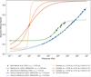 |
Fig. 1 Dependency of the VFF on the compressive stress. The three curves on the left that cross at p = 10 Pa are artificial displays of Eq. (5), each with pm = 10 Pa, φs = 0.15, and φd = 0.64 but with different values of ∆, namely 0.1,0.5, and 0.9, respectively. The two curves on the right are fit functions of Eq. (5) to the data of Meisner et al. (2012) and Omura & Nakamura (2021), respectively. Both datasets were fitted using Method B2, while the data of Omura & Nakamura (2021) were additionally fitted using Method B3 to account for the anomalous increase in VFF observed at pressures above ∼2 ∙ 106 Pa. Solid lines indicate the measured pressure range, whereas dashed lines represent extrapolations of the fitted compression curves beyond the measurement range. All turnover pressures pm are marked by filled circles. |
3 Determination of the turnover pressure as a function of grain size
We extensively searched the literature for data with which the stratification of granular matter under gravitational selfcompaction can be derived. In the best cases, these data comprise the free parameters of the regolith stratification model (Eq. (9)), namely φs, φd, pm and ∆, respectively. Table 1 lists all investigations we could find. They are discussed in more detail hereafter. To enable a fair comparison between quasi-monodisperse and polydisperse dust samples, we use the median volume-equivalent radius as our particle-size metric. Kreuzig et al. (2024) showed that this choice yields the best agreement in the tensile strength of micro-granular dust samples. Because both tensile strength and compressibility are governed by inter-particle forces, this metric is well justified.
3.1 Re-analysis of literature filling-factor data with respect to turnover pressure (Method A)
The data in Table 1 using Method A refer to measurements of the bulk VFF of granular samples as a function of grain size. We used these data and re-analysed them utilising the regolith stratification model (see Sect. 2) to derive the turnover pressure pm for a meaningful range of transition widths ∆. However, we restricted our analysis to the size range r > 5 μm, because for smaller sizes particle clumping leads to unrealistically low filling factors. One has to note, however, that for sizes r ≫ 100 μm the densest state is already reached within the first few monolayers so that the particle-size sensitivity is lost.
As the experiments were carried out in containers of finite dimensions, the Janssen effect must be taken into account, which refers to the phenomenon observed in granular materials for which the vertical stress induced at the base of a cylindrical container of granular particles is less than what might be expected based solely on the weight of the material above it (Sperl 2005). This effect occurs due to the interactions among the particles, particularly lateral forces and friction, which redistribute the stress. As a result, the effective stress at the base at depth H can be significantly reduced and is given by
![Mathematical equation: p_\mathrm{eff}(H)=\bar{\rho}~ g ~H \frac{D}{4~ k ~\mu~H} \left[ 1-\exp\left( -\frac{4~ k~ \mu ~H}{D}\right) \right].](/articles/aa/full_html/2026/03/aa58471-25/aa58471-25-eq14.png) (11)
(11)
Here, ρ̄, D, k, and μ are the average bulk density of the sample, the diameter of the container, the ratio of lateral to vertical pressure (0 ≤ k ≤ 1) and the coefficient of friction (between powder and wall), respectively. The coefficient of friction is μ = 0.16 for glass beads (Tang et al. 2019) and μ = 0.47 for alumina (Kikuchi et al. 2015). Due to a lack of data about the parameter k, we used k = 1 as an upper limit for a maximum possible Janssen effect. Thus, these estimates are naturally upper limits for the stress reduction and cannot be easily implemented into the density stratification dealt with in this paper as long as the exact value of the parameter k is not known. However, the estimates provide us with a strict lower limit for the turnover pressure function pm ( r).
We also studied the enhanced Janssen effect for conical containers. A conical shape leads to a maximum vertical pressure at some intermediate depth and to a negligible pressure at the tip of the cone (Ivchenko 2023). Calculations using the geometry of the container used by Yu et al. (1997) show that, due to the steepness of the walls and the truncated shape, this results in only a very small correction to the Janssen effect, and thus we do not consider it here.
As the works listed in Table 1 under Method A measured the average (or bulk) density ρ̄, which is analogous to the average VFF φ̄, we tabulated the function Z(φ) (Eq. (10)) for φs = 0.15, φd = 0.64, ∆ = 0.1,0.2,..., 1.3 for φ ∈ [φs,φd] with a small step size δφ. Starting with Eq. (9), we derived the average filling factor of a sample of height H in the following way:
 (12)
(12)
where φmax = φ(H) is the VFF at the bottom of the sample, i.e. for x = H. It is important to note that φmax is the VFF actually reached at the bottom of the sample, whereas the maximum pressure pmax is a virtual value and is defined for φ = 1. In addition, it should be noted that the integral on the RHS of the last equation depends only on φmax and ∆.
Next, we calculated φmax by equating the expression  in Eqs. (10) and (12) for x = H:
 (13)
(13)
For this φmax, we then calculated  using Eq. (10),
 (14)
(14)
For each grain radius r and for each ∆ = 0.1, 0.2,..., 1.3, we thus obtained a unique value of  .
.
As we knew the values of g, ρgrain, and H, this approach yielded a pm(r) relation for every value of ∆. We applied this recipe for the two extreme values of pmax, namely for the case of absent Janssen effect,
 (15)
(15)
and for the case of the maximum Janssen effect (see Eq. (11)),
![Mathematical equation: p_\mathrm{max}^-=p_\mathrm{max}^+~ \frac{D}{4~ k ~\mu~H} \left[ 1-\exp\left( -\frac{4~ k~ \mu ~H}{D}\right) \right],](/articles/aa/full_html/2026/03/aa58471-25/aa58471-25-eq22.png) (16)
(16)
with k = 1. This then yielded the upper and lower limits of the pm(r) relation, namely pm+(r) and pm−(r), representing the cases k = 0 (no pressure transfer to the side walls) and k = 1 (maximum pressure transfer to the side walls), respectively.
In the following paragraphs, we briefly describe the data used in our study, first for silica (glass, quartz, SiO2) and then for alumina (Al2O3). Both minerals are major chemical constituents of the lunar regolith, with abundances of ~40-50% (SiO2) and ~ 10-30% (Al2O3), respectively (see e.g. McKay et al. 1991; Wang et al. 2025). The data are summarised as Method A in Table 1.
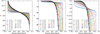 |
Fig. 2 Function Z(φ; ∆, φs, φd) in Eq. (10) with fixed values φs = 0.15, φd = 0.64, and ∆ = 0.1,0.2,... 1.3 in logarithmic (left) and two different linear scalings (centre and right). The respective depth function x(φ; ∆, φs, φd) can be derived by x = (Z pm)/(g ρgrain) using Eq. (10). |
Summary of the experimental data on granular compaction used in this work.
3.1.1 SiO2
Omura et al. (2016) poured irregular silica sand with three different mean radii between r = 6.5 μm and r = 38.5 μm into cylindrical containers with D = 58 mm diameter and H = 33 mm height and measured the porosity of these loose granular packing (see their Figure 4) before they conducted compression experiments (see Sect. 3.2).
Gan (2003) used spherical glass powders, dried at 110°C, with 11 different median radii in the range r = 8.2-113 μm and poured them through a funnel into a cylindrical container with a height of H = 30 mm and diameter of D = 21 mm. No tapping was employed. The porosity was then determined by weighing the sample (see their Figure 3.4).
Parteli et al. (2014) utilised nine spherical polydisperse glass powders with mean radii in the range r = 1.9-26 μm. About 80 cm3 of powder were poured through a funnel into a cylindrical container with a diameter of D = 35 mm. No tapping was employed. The packing density was then determined by measuring the powder bulk volume and weighing the sample (see their Table 1 and Figure 3).
3.1.2 Al2O3
Yu et al. (1997) used white fused alumina powders, dried at 100°C, with median radii in the range r ≈ 1.4-27 μm. The powders were poured through a funnel into a slightly conical container with a height of H = 70 mm and upper/lower diameter of D = 57/44 mm. The packing density was then determined by weighing the sample. Yu et al. (1997) also tapped their samples and measured the packing density again, but we here refer to the untapped VFF.
Omura et al. (2016) performed the same experiments as described in Sect. 3.1.1 with alumina particles and radii in the range 2.25-38.5 μm.
3.2 Re-analysis of literature compression data with respect to turnover pressure (Method B)
Studies that analysed the VFF as a function of pressure are categorised as Method B in Table 1. To enable a consistent comparison between the different measurements, a uniform representation of grain size is required. Some studies reported mean grain sizes, while others provided median grain sizes based on volume (mass) or count. Therefore, all values were standardised to the median radius of the cumulative volume distribution (r50v), because this is the only grain size metric that can be derived for all materials. In addition, the 10th and 90th percentiles (r10v and r90v) are determined to account for the polydispersity of the materials. The resulting percentile values for each study are summarised in Table 2, and their derivation is described below.
The monodisperse material analysed by Güttler et al. (2009) is identical to the one investigated by Poppe & Schräpler (2005), who published a histogram showing grain diameter versus number fraction obtained from scanning electron microscopy. By extracting the number of grains in each size class and normalising the values, the cumulative count fraction was calculated, and a plot of cumulative count fraction versus grain diameter was constructed. To derive the median volume-based diameter, the number of grains in each size class was multiplied by the corresponding particle volume and cumulated, yielding a cumulative volume fraction curve, from which the values of d10v, d50v and d90v were extracted. These diameter values were then converted to radii, yielding r10v, r50v and r90v.
For the material examined by Machii et al. (2013) no histograms were provided. Instead, we re-examined the silica particles used by Machii et al. (2013) ourselves. High-resolution SEM images were analysed using the Fiji/ImageJ software. From the cumulative volume distribution, we derived r10v, r50v and r90v.
The material studied by Meisner et al. (2012) was identical to the one examined by Kothe et al. (2013), who measured both the median volume and median count diameters using a laser diffractometer. The 10th, 50th, and 90th percentiles were extracted directly from their Figure 3 and subsequently converted to radii.
In the case of the three materials analysed by Schräpler et al. (2015), the published number-fraction histograms were used. The values of r10v, r50v, and r90v were therefore calculated using the same method as applied for the material from Güttler et al. (2009).
For the materials studied by Omura & Nakamura (2017), Omura & Nakamura (2021) and Omura et al. (2025, pers. comm.), the grain size distributions were measured using a laser diffractometer and diagrams showing grain size versus cumulative volume fraction were available in the publications or provided directly by the authors. Therefore, the 10th, 50th, and 90th percentiles were extracted directly from these plots and converted to radii.
Due to variations in the way different authors presented and visualised their data, Method B was implemented using three distinct approaches to determine the turnover pressure pm and the transition width ∆. These approaches were denoted B1, B2, and B3, respectively. All of them rely on Eq. (5) to derive the turnover pressure and the transition width. Only the studies of Güttler et al. (2009) and Schräpler et al. (2015) reported explicit turnover pressures, VFFs, and transition widths for their measurements. For the remaining datasets, the methods described below were employed.
Approach B1 involved visual fitting of Eq. (5) to a plot of the VFF versus the logarithmic pressure. This method was applied to the data of Machii et al. (2013), because the original publication already displayed a suitable log-pressure versus porosity diagram.
The second approach, B2, was applied when the original measurements were not presented using Eq. (5) nor visualised in a VFF versus logarithmic pressure plot, as in the case of Meisner et al. (2012), Omura & Nakamura (2017), Omura & Nakamura (2021), and Omura et al. (2025, pers. comm.). Depending on whether the data was presented as discrete data points or as a continuous curve, the WebPlotDigitizer tool was used to manually extract discrete (p, φ) pairs or to extract data points at regular intervals along the compression curves from digitised figures. Eq. (5) was then fitted to the extracted data points using SciPy’s curve_fit routine, which employs the Trust-Region Reflective algorithm, with specified parameter bounds (0 ≤ φ ≤ 1). This yields the best-fit turnover pressure pm, transition width ∆, and VFFs φ s and φd.
Approach B3 was applied in cases where the regular fitting routine yielded physically implausible values for the VFF, or when the compression curves displayed uncharacteristic behaviour. This occurred for the studies of Machii et al. (2013), Omura & Nakamura (2017), Omura & Nakamura (2021) and Omura et al. (2025, pers. comm.), whose measured compression curves exhibited an unusual second increase in VFF at higher pressures of 105−106 Pa. This could be attributed to the material displacement between the wall of the container and the compressing piston, because, for example, Omura & Nakamura (2021) described a 0.8 mm gap between the container and the piston, through which the material could have crept upward under high pressure. When the original fit was performed using Approach B1, Approach B3 involved manually constraining the parameters φs and φd to physically reasonable values, with data points corresponding to the second increase in the VFF excluded in the refit. This approach was applied to the data from Machii et al. (2013). Conversely, when the original fit had been performed with Approach B2, Approach B3 consisted of rerunning the fitting routine with explicit bounds on φs and φd based on observed trends in the experimental data and known physical limits for φs and φd. This was applied to Omura & Nakamura (2017), Omura & Nakamura (2021) and Omura et al. (2025, pers. comm.).
For all approaches except B1, the standard deviation of the fitted turnover pressure was calculated from the diagonal elements of the covariance matrix. A more precise uncertainty determination was not possible because (i) some studies did not report or visualise any uncertainties, (ii) the uncertainties were too small to be significant or (iii) the original visualisations were too imprecise or unclear to assign error bars to specific points.
All determined values for the turnover pressure and transition width are listed in Table 1 under Method B. Figure 1 shows examples of the fitting results and Fig. 3 illustrates the values along with their corresponding standard deviations.
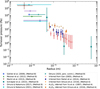 |
Fig. 3 Obtained values of the turnover pressure, pm, as a function of grain radius, r, as listed in Table 1. It should be noted that we used transition widths in the range ∆ = 0.1... 1.3 for all data points analysed using Method A so that the relatively large range of the derived pm values is not an error range but denotes the range of the formal results. Most of the values obtained refer to silica samples. For comparison, the turnover pressures inferred from the Al2O3 samples are illustrated as well. |
3.3 Synthesis: Derivation of the turnover pressure as a function of grain size
The data derived in Sects. 3.1 and 3.2 for individual values of the SiO2 turnover pressure pm are now combined into a single pm(r) data set that can be used in the stratification model (Eq. (9)) for the Moon and other atmosphere-less planetary bodies. Figure 3 displays the final data with all estimated uncertainties in pm and r. Please note that the maximum possible Janssen effect, as discussed in Sect. 3.1, is not yet taken into account in this dataset. For comparison, the turnover pressure inferred from the Al2O3 samples is illustrated as well. Individual radius variations of the samples are shown as horizontal error bars in Fig. 3. It should be noted that for all data points analysed through Method A (see Sect. 3.1), we used the transition width as a free parameter and varied it over ∆ = 0.1,0.2,..., 1.3 so that we also received a corresponding range of pm values. Larger values of the transition width ∆ lead to lower values of the turnover pressure for r ≳ 10 μm. For the smallest grain radii considered here, r ≲ 10 μm, larger values of ∆ lead to higher values of the turnover pressure. Thus, it should be noted that the relatively large range of derived pm values for Method A shown in Fig. 3 does not represent the error, but denotes the range of formal results obtained for pm. For the data sets from Gan (2003) and Parteli et al. (2014), we were unable to find a solution for the turnover pressure at a transition width value of ∆ = 0.1 and therefore only plotted solutions for ∆ = 0.2,..., 1.3.
When taking all data together, it can be seen that the turnover pressure extends over six orders of magnitude, while the size range covers about three orders of magnitude. Most of the data points relate to silica samples. Thus, in the following analysis, we only used the silica data.
In order to arrive at a mathematical description for pm (r), we first fitted a simple power-law function,
 (17)
(17)
to the data, taking the individual r values as the median volumeequivalent radii.
As the slope of the function pm (r) in the double-logarithmic plot of Fig. 3 is seemingly steeper for small particle sizes than for large grains, we also fitted the data with a double-power-law ansatz
 (18)
(18)
with α2 > β2. Thus, for small grains the first term on the RHS of Eq. (18) dominates, whereas for large grains the second term is more important.
To account for the large spread of pm values, we actually fitted the logarithm of Eqs. (17)-(18) to the log10 pm data. We tried various fitting methods, including the least squares, orthogonal distance regression, and taking individual x- or y-error bars into account. We also tried to take into account our knowledge of the range of possible values for the transition width ∆. A look into Table 1 (Method B) shows that most empirical values for ∆ fall into the range ∆ = 0.4... 0.6. Thus, we also fitted the whole data set with this restriction, meaning that the turnover pressure values obtained by Method A were restricted to this narrower range in transition width ∆. It turned out that the two best fits for these data were those obtained by the least-squares method and ignoring individual error bars. The results are shown in Fig. 4 and read A1 = 1.30 ∙ 10−8, α1 = 2.01 ± 0.15 (left panel, solid line) and A2 = 1.88 ∙ 10−13, α2 = 2.85 ± 0.61, B2 = 3.53 ∙ 10−5 and β2 = 1.23 ± 0.47 (centre panel, dashed curve). Because we fitted the logarithm of Eqs. (17)-(18), the uncertainties for A1 and A2, B2 can only be noted as log10(A1) = −7.89 ± 0.77 and log10(A2) = −12.70 ± 3.64, log10(B2) = −4.45 ± 1.99. To illustrate the effect of the uncertainty of the fit parameters, Fig. 4 also shows the 1σ and 2σ uncertainties of the corresponding fits. Varying the fitting method (e.g. including individual error bars or the whole range of transition widths ∆) changed for the single power-law α1 in the range α1 ≈ 1.9-2.3 and for the doublepower-law α2 and β2 in the range α2 ≈ 2.7-3.4 and β2 ≈ 0-1.3. Taking into account the maximum possible Janssen effect for the turnover pressure values determined by Method A (see Sect. 3.1) had only a minor effect on the derived values of α1, α2 and β2 and the values lie well within their respective error bars.
As a measure for the goodness of the two fits, we determined the value
 (19)
(19)
with pm,i, fpm,j, n and mj being the data points, the corresponding fit values, the number of data points and the number of fit parameters (mj = 2, 4 for the above two fit functions), respectively. We found the following values:  and
and  .
.
These values mean that the average deviation between the data points and the fit function are a factor of 3.80 and 3.43, respectively. Thus, Eq. (18) fits the data only slightly better than a single power law.
In conclusion, the data seem to follow closely a single power law with a slope of −2. Yet, there is an indication that for smaller particles, this slope is slightly steeper than −2 and becomes shallower than −2 for larger grain sizes. However, the effect of this non-constant slope is quite small in the size range 10−6 m ≤ r ≤ 10−4 m and only exceeds a factor of a few outside these limits. We also note that (α2 + β2) /2 ≈ α1 ≈ 2, which emphasises that the average slope of the pm(r) curve is —2.
Based on the findings above and due to theoretical reasons (see Sect. 5), we also fitted a simple power-law function with a fixed slope of −2,
 (20)
(20)
to the data, which resulted in A3 = 1.48 ∙ 10−8 with log10(A3) = −7.83 ± 0.10 and  (or, an average deviation of a factor 3.71), even slightly better than Eq. (17). The resulting fit curve is also illustrated in the right panel of Fig. 4 (dash-dotted line).
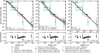 |
Fig. 4 Result of the fitting procedure of the turnover pressure, pm, as a function of grain radius, r, for all SiO2 samples using Eq. (17) (left, solid line), Eq. (18) (centre, dashed curve), and Eq. (20) (right, dash-dotted line), respectively. The fits were performed using the least-squares method and ignoring individual error bars. The turnover pressure values obtained by Method A were restricted by the condition ∆ = 0.4...0.6. The logarithmic residuals are illustrated in the lower panels, together with the individual ranges in pm (Method A) or error bars (Method B) of the data points. The fit results are noted in the respective legend. The shaded regions illustrate the 1σ and 2σ uncertainties of the respective fits. |
4 Constraints on the transition width
From the data shown in Table 1 (Method B, last column), we can see that the derived values for the transition width extend over a range Δ = 0.46-2.29. However, there seems to be a trend that Δ increases with increasing width of the size distribution. The latter can be seen in the last columns of Table 2. Samples with widths r90v/r50v ≲ 10 have values in the range ∆ = 0.4-0.6, whereas size ranges r90v/r50v ≳ 10 possess transition widths ∆ ≳ 1. Moreover, for the data set from Gan (2003) and Parteli et al. (2014), we were unable to find a solution for the turnover pressure at a transition width value of ∆ = 0.1 and therefore suggest that also such a small value for the transition width should be considered unlikely. We conclude that for moderately wide size distributions ∆ can be well constrained by ∆ = 0.4-0.6.
5 Discussion of the results
Comparison to a grain aggregate compression model. Tatsuuma et al. (2023) used numerical simulations of cohesive monomer aggregates to measure compressive strength across a wide range of VFFs, capturing both very porous and compacted regimes. They propose a unified empirical formula that links compressive strength to filling factor as well as monomer and material properties. Their main result (their Eq. (11)) reads as
 (21)
(21)
Here, γ and φd are the surface energy of the grain material and the maximum filling factor at high compression, respectively.
If we only consider the dependency on the VFF and taking into account that Tatsuuma et al. (2023) started their compression simulations with an initial VFF of φini ≈ 0, we can see that this is equivalent to the expression in Güttler et al. (2009) (see Eq. (8) above) if φini = φs = 0 and ∆ ln(10) = 3 or ∆ = 1.30.
We re-fitted the data using Eq. (17), but now under the condition that ∆ = 1.3 for all data points derived by Method A. We received values of A1 = 1.40 ∙ 10−11 and α1 = 2.51 ± 0.19 and  . The fit quality is much reduced compared to the one shown in Fig. 4 (left) and the slope is 2.7 standard deviations off the expected value (see below) so that we consider this choice for ∆ suboptimal.
Moreover, it is interesting to note that Eq. (21) predicts that the compression required to achieve a constant VFF is Pcomp(φ = const) ∝ r−2. This fully agrees with our findings as shown in Sect. 3 for ∆ = 0.5. Thus, we experimentally confirmed the grain size dependency in the result of Tatsuuma et al. (2023). Tatsuuma et al. (2023) provide a universal, microphysics-based relation between external pressure and aggregate VFF across a wide compaction range by resolving monomer-monomer contacts and their rearrangements, and by scaling with the rolling energy. Conditions for the constituent grains and contact physics are that (i) monomers are ideal, identical spheres (monodisperse); (ii) cohesion is purely of van der Waals type so that contact mechanics follow the Johnson-Kendall-Roberts (JKR) theory for elastic adhesive spheres (Johnson et al. 1971); (iii) energy-dissipating contact modes are rolling, sliding, and twisting; each is governed by a critical displacement/threshold, with fixed material parameters; (iv) material constants are uniform and temperature-independent; the characteristic rolling energy sets the strength scale; and (v) no sintering, melting, cementation, moisture, or chemical bonding take place; no electrostatic charging forces beyond the van der Waals cohesion play a role. The close agreement between the model results and our empirical findings suggest that all of the above conditions are well-matched. In particular, the condition for ideal spheres is remarkable as it implies that surface-roughness effects are negligible. This is only the case, when the roughness size scale is much smaller than the contact size scale between touching particles. The contact radius according to the JKR model ranges between ~20 nm and ~2 μm for particle radii between 1 μm and 1 mm; the mutual indentation length scale for the same range of particle radii reach from ~1 nm to ~10 nm. If roughness effects dominated the contact between the spheres and if we assume that surface asperities are independent of particle size, the resulting scaling would be Pcomp(φ = const) ∝ r−3, which clearly contradicts our observation. Thus, we conclude that surface roughness with a particle size-independent roughness scale is negligible over the observed range of grain radii. This is also in agreement with empirical roughness measurements of fine particles as collected by Güttler et al. (2012) in a literature survey. However, if the roughness length scale is proportional to the particle size, we would expect the observed Pcomp(φ = const) ∝ r−2 behaviour. In that case, the absolute values for the turnover pressure would be systematically shifted to smaller values. This would be indistinguishable from a smaller Hamaker constant (or surface energy) so that we cannot exclude surface roughness effect completely.
Influence of the grain material on the turnover pressure. It is natural to assume that the turnover pressure depends linearly on the cohesion force between the grains. The latter can be expressed either by the Hamaker constant A or, completely equivalently, by the surface energy γ ∝ A of the material (see Eq. (21) above). Kiuchi & Nakamura (2014, 2015) assumed the JKR contact model and thus for the compressibility of a granular medium obtained a dependency on r2/A. Taking the main result of this paper that pm ∝ r−2 suggests that pm ∝ A. Thus, the final result of our analysis can be simply expressed as
 (22)
(22)
where ASiO2 is the Hamaker constant of silica (see below). Eq. (22) should be valid for a wide range of Hamaker constants, as long as the main force between grains in contact is the van der Waals attraction.
Alumina versus silica. In the lunar regolith, silica and alumina have mass fractions of 40-50% and 10-30%, respectively (McKay et al. 1991, their Tables 7.15 and 7.16). Thus, they comprise the major chemical constituents of the lunar regolith. According to French (2000, their Table III), the surface-vacuum-surface Hamaker constants of SiO2 and Al2O3 are ASiO2 = (0.682 ± 0.002) × 10−19 J and AAl2O3 = (1.649 ± 0.008) × 10−19 J, respectively. The ratio of both is AAl2O3/ASiO2 = 2.4 and this at least qualitatively explains why the turnover pressure of Al2O3 lies systematically by a factor of a few above the average SiO2 value (see Fig. 5).
Influence of the grain size distribution on the compaction behaviour of the regolith. Consistent with established granular packing theory and simulations, the polydispersity of a grain size distribution largely sets the maximum VFF, i.e. the RCP limit, with broader distributions achieving higher RCP VFFs (see e.g. Farr & Groot 2009; Desmond & Weeks 2014). The distribution width may also influence the characteristic turnover pressure of the compaction curve, because fine particles can form interconnections between larger grains that allow contacts to roll more easily; such a mechanism is consistent with micromechanical rolling-friction arguments developed for grain contacts. However, the data compiled in this work show no clear evidence of a systematic dependence of the turnover pressure on polydispersity. Instead, our measurements indicate that increasing the width of the grain size distribution primarily broadens the transition width ∆ of the VFF-pressure relation, an effect that should directly modulate the depth-dependent stratification of regolith under self-compression. Indirectly, the apparent absence of the dependency of pm on the width of the size distribution confirms that our choice of the grain size measure, namely the volume-equivalent median radius, was well justified.
Influence of other grain properties on the turnover pressure. Works on the maximum VFF for monodisperse non-spherical convex (Zou & Yu 1996) and non-convex particles (Faure et al. 2009) revealed that the maximum VFF depends on the grain shape and can be, depending on the aspect ratio of the grains, very different to the value assumed in this work (φRCP = 0.64). Inter-particle friction also plays a decisive role for the maximum VFF: frictionless grains have the highest maximum VFF, decreasing by a few percent for higher inter-grain friction (Salerno et al. 2018). Thus, the lower boundary condition used by us, φd = 0.64 is certainly just an estimate and needs to be adjusted when the respective grain properties are known.
Comparison to previous works. Schräpler et al. (2015) proposed a grain size dependency of the turnover pressure of pm ∝ r−4/3, which is a major difference to pm ∝ r−2 found in this work. In their thermophysical model for the lunar regolith, Bürger et al. (2024) adopted the former relation, but introduced two different absolute calibrations for the turnover pressure (see Fig. 5). However, for the grain radii relevant for the lunar regolith (r ≈ 20... 50 μm; McKay et al. 1991), the difference to the lower of the two curves used by Bürger et al. (2024) (their Figure 2) is very small (less than a factor of two for r = 20 μm; negligibly small for r = 50 μm). When using the double-power law fit (Eq. (18)), the difference is even smaller and practicably negligible for all grain sizes 20 μm ≲ r ≲ 1 mm. Thus, we do not expect major differences in the outcome of the thermophysical modelling.
Comparison to empirical density stratifications for lunar regolith. Fig. 6 illustrates the resulting stratification profile for the lunar regolith assuming a grain radius r = 35 μm, transition width ∆ = 0.5, a density of the solid material ρgrain = 3000 kg m−3 and the turnover pressure as determined in Eq. (22) with A = ASiO2. The function is compared with empirical stratification models for the lunar regolith introduced in Sect. 1 (Eqs. (1)-(4)). We note that the stratification model in this study shows lower bulk densities for depths ≲1 cm and higher bulk densities for depths ≳2 cm than the other functions. The functions are based on the Apollo core tubes which measured the average bulk density in ~0-30 cm and ~30-60 cm depth. These measurements do not enable a resolution of the upper centimetre of the regolith. Therefore, they do not contradict our model, which is based on the principles of granular packing. Concerning the slightly higher bulk densities in the deeper layers, we note that the bulk density in our model depends on the assumed grain density and a variation of this value also allows for lower bulk densities in the deeper layers. In principle, the returned Apollo 15-17 core samples suggest a bulk density of the lunar regolith in the range 1360-2290 kg m−3 (Carrier et al. 1991), and our stratification profile lies within this range. However, the typical average values for a depth of 0-60 cm are 1610-1710 kg m−3 (Mitchell et al. 1974). Finally, in Sect. 6 we show that the presented bulk density profile in this study is able to match the measured depth of astronaut footprints on the lunar surface.
A comparison to the other stratification profiles shown in Fig. 6 reveals that for an assumed material density of ρgrain = 3000 kg m−3 Eq. (1) provides the limiting values of φ(x = 0) = 0.37 and φ(x → ∞) = 0.60, Eq. (2) results in φ(x = 0) = 0.43 and φ(x → ∞) = 0.64, Eq. (3) in φ(x = 0) = 0 and φ(x → ∞) → ∞, and Eq. (4) in φ(x = 0) = 0.27 and φ(x → ∞) → ∞, respectively, whereas our stratification model uses physical limits of φ(x = 0) = 0.15 and φ(x → ∞) = 0.64. Even if one allows for uncertainties on the grain density, φ(x = 0) = 0 and φ(x → ∞) → ∞ are unphysical. Also VFFs at the surface of 0.43 or 0.27 are not in agreement with data by Szabo et al. (2022) from modelling energetic neutral atom emission of the upper lunar regolith layers. Only the lower boundary conditions with VFFs of 0.60 and 0.64 seem plausible. Thus, we believe that our stratification model with upper and lower boundary VFFs of 0.15 and 0.64, respectively, can be regarded as realistic.
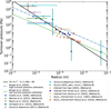 |
Fig. 5 Comparison between the turnover pressure-grain size relations used by Bürger et al. (2024) (dashed and dash-dotted lines) and the main result of this work (Eq. (20), solid line). In addition to the data obtained for SiO2, the turnover pressure inferred from the Al2O3 samples are illustrated as well but were not used for fitting. It should be noted that we only used transition widths in the range ∆ = 0.4...0.6 for all data points analysed using Method A. |
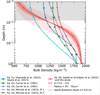 |
Fig. 6 Comparison of different stratification models for the lunar regolith. The models and respective equations from the literature are detailed in Sect. 1. For the bulk density model by Vasavada et al. (2012), we used H′ = 0.07 m from Hayne et al. (2017). For the stratification model in this study (Eq. (9)), we inserted the turnover pressure as described in Eq. (17) with a slope of −2, a transition width of ∆ = 0.5, a particle radius of 35 μm, and a grain density of ρgrain = 3000 kg m−3. The effect of varying transition width (∆ = 0.4...0.6) and particle radius is illustrated as well, with a range of 20-50 μm as motivated by McKay et al. (1991). |
6 Applications
Thermophysical models of lunar regolith. As introduced in Sect. 1, surface and subsurface temperatures of granular surfaces are very sensitive (especially during nighttime) to grain size and density stratification. Thermophysical models predict surface and subsurface temperatures, and matching of the simulated temperatures with measured ones allows the properties of the granular material to be constrained. Bürger et al. (2024) developed a microphysical thermophysical model for the lunar regolith, which describes the density stratification based on the model by Schräpler et al. (2015) presented in this study (Eq. (9)), i.e. as a function of grain radius, transition width, surface and deep layer bulk density and turnover pressure pm ∝ r−4/3 (see Fig. 5). In addition, it uses a grain size and volume-filling-factor dependent thermal conductivity (Gundlach & Blum 2012). Therefore, the refined description of the turnover pressure as a function of grain size, pm ∝ r−2 (Eq. (20)) will lead to a more accurate prediction of lunar regolith properties. As already stated above, when referring to the lower turnover pressure calibration used in Bürger et al. (2024) and shown in Fig. 5 (dashed line), we do not expect major differences in the derived temperatures, because the two functions are quite similar in the relevant grain-radius range. However, in addition, the thermophysical model suffers from a degeneracy of the free parameters, and thus the absolute definition of the turnover pressure and the narrower range of the transition width ∆ derived in this study will contribute to further restrictions of the solution space.
Predicting the depth of astronaut footprints on the Moon. A natural test of our lunar regolith stratification model are the boot prints left by the Apollo astronauts that are well documented (NASA 1971; Mitchell et al. 1974). Analysis of more than 700 actual footprints left by the astronauts on the lunar surface revealed an average boot print depth of approximately 0.8 cm (calculated from Fig. 3−18 in Mitchell et al. 1974). Based upon our regolith stratification model, we calculated the expected depth of an astronaut’s footprint on the Moon as described in the following:
We assumed a one-foot pressure of pfoot,0 = 7 kPa (NASA 1971). Taking the footprint size with a length of 33 cm and width of 12.5 cm (as illustrated in Fig. 3−18 in Mitchell et al. 1974) into account, we arrived at a compressive force of ~290 N. Due to the force chains in the underlying regolith, the area over which the force acts increases quadratically with increasing depth x. Taking into account the finite crosssection of the footprint at x = 0, the pressure thus decreases with increasing depth by pfoot = pfoot,0/(1 + — )2. Here, rfoot is the characteristic boot size (radius), which we calculated through
 , i.e. assuming a circle with the same area as the rectangular footprint.
We approximated the maximum depth xmax to which the load of the astronaut penetrates by equating pfoot with the lithostatic pressure in that depth, i.e. the inverse of Eq. (7), xmax = x(pfoot). We also determined the VFF φ(xmax) in that depth, applying Eq. (9).
In the following, all depths x < xmax were compacted to the maximum packing density φ(xmax), resulting in a reduced layer thickness of
 .
.Finally, the footprint depth was calculated by dfoot = xmax - d.
In the calculations, we used the final result of our turnover pressure-radius relation presented in Eq. (22). Assuming a grain radius r = 35 μm, transition width ∆ = 0.5 and density of the solid material ρgrain = 3000 kg m−3, this results in a predicted footprint depth of dfoot ≈ 1.5 cm for our stratification model. Varying the transition width within ∆ = 0.4... 0.6 shows that the lowest value ∆ = 0.4 leads to a prediction of a shallower footprint depth of dfoot,∆=0.4 ≈ 1.3 cm. The variation in grain radius between r = 20... 50 μm (McKay et al. 1991) for fixed ∆ = 0.5 shows that the highest value r = 50 μm also leads to a prediction of a shallower footprint depth of dfoot,r=50 μm ≈ 0.89 cm. We find the best agreement with the Apollo boot print depths for r = 46 ... 50 μm, ∆ = 0.40... 0.45 with dfoot ≈ 0.80 ± 0.01 cm, for which we then get in all cases xmax ≈ 24 cm. We also evaluated the predicted boot print depth for all other stratification models (Eqs. (1)-(4)). The corresponding depth-density profiles are illustrated in Fig. 6. However, as those models do not include a dependence of the bulk density with pressure, we assume the same xmax ≈ 24 cm as calculated from our stratification model, which led to the best agreement with the measured boot print depths, and calculate φ(xmax), d and dfoot as described above. This results in dfoot,eq.1 ≈ 2.4 cm for Eq. (1), dfoot,eq.2 ≈ 1.9 cm for Eq. (2), dfoot,eq.3 ≈ 1.3 cm for Eq. (3), dfoot,eq.4,fit1 ≈ 3.1 cm for Eq. (4) (fit 1) and dfoot,eq.4,fit2 ≈ 1.4 cm for Eq. (4) (fit 2). Thus, the stratification models by Carrier et al. (1991) (Eq. (3)) and Mitchell et al. (1972) (Eq. (4), fit 2) predict a boot print depth that is approximately 1.5-2 times greater than measured, while all others result in a factor of 2-4 between the measured and predicted bootprint depth. Although the overall calculation of the expected depth of astronaut footprints involves a series of approximations, such as the relationship of the astronaut pressure-depth dissipation, the shape of the boot and the lithostatic pressure-depth dependence of the other stratification models, this exercise shows that the studied stratification model (Eq. (9)) is in principle able to predict the measured depth of astronaut footprints on the lunar surface.
Importance of the regolith stratification model for small Solar System bodies. Using our regolith stratification model in the form expressed in Eq. (10), we could estimate for which celestial objects the regolith is not stratified but possesses the same VFF from the surface to greater depths. This is the case when the function Z obtains for the most relevant values ∆ = 0.4-0.6 almost constant VFFs of φ ≈ φd. From Fig. 2 one can see that this is the case for Z ≳ 10. This means that the regolith exhibits the typical stratification pattern only for values Z ≲ 10. Assuming Z ≳ 10, a typical material density of ρgrain = 3000 kg m−3, surface accelerations of g = 100,10−1,10−2,10−3 m s−2 (equivalent to celestial bodies of sizes ~ 103,102,101,100 km) and setting x = r as the threshold depth between important and negligible stratification, we find r ≳ 0.4, 0.8, 1.7, 3.6 mm, r ≳ 0.8,2.2,6.2,17.3 mm and r ≳ 0.4,0.8,1.7,3.7 mm, when using the three pm(r) relations from this paper, Eqs. (17), (18), and (20), respectively. Thus, any kind of thermophysical or mechanical modelling of the regolith of small Solar System objects needs to take stratification into account if the grain size is below the values given above.
7 Summary and conclusion
The regolith stratification model developed by Schräpler et al. (2015) and Bürger et al. (2024) describes the depth dependency of the packing density (or VFF) for given values of the gravitational acceleration and the material density of the regolith grains (see Eq. (9)). It possesses four free parameters: the VFF at the surface (φs) and at great depths (φd); the grain size-dependent turnover pressure, pm(r); and the logarithmic transition width between low and high VFFs (∆). In this work, we mainly determined pm(r) and constrained ∆.
We compiled and analysed literature data on the bulk packing fraction of silica and alumina powders (Table 1, Method A) with the static stratification model (Sect. 2, Eq. (9)), treating the transition width (∆) as a free parameter (Sect. 3.1), and we examined quasi-static compaction measurements (Table 1, Method B; Sect. 3.2). From these datasets, we derived the turnover pressure, pm(r), across a wide size range, from sub-micrometre to sub-millimetre values (see Fig. 3). A single power-law model, i.e. pm(r) ∝ r−α (see Eq. (17)), following Tatsuuma et al. (2023), with a slope of α ≈ −2 reproduces the data reasonably well (see Fig. 4, left and right). However, the compiled measurements are in slightly better agreement with a steeper slope than −2 for small grains and a shallower slope for larger grains. Accordingly, a two power-law representation (Eq. (18)) provides a modest improvement, yielding a slightly lower χ2ed (Eq. (19)) than the single power law (see Fig. 4, centre). The data presented and our analysis also suggest modest values for the logarithmic transition width, ∆ = 0.4... 0.6, although some of the measurements are in better agreement with ∆ > 1, particularly those with wide grain size distributions.
Taken together, our verified stratification framework (Eq. (9)) combined with the approximate relation between turnover pressure, material properties, and grain size (Eq. (22)) constitute a ready-to-use prescription for modelling planetary regolith and other loose particulate packings in an arbitrary gravitational field. The approach is valid for grain sizes from micrometres to millimetres and enables consistent forward modelling of the stratification of planetary regolith in all gravitational environments, from small to large objects.
Acknowledgements
G.M. acknowledges support by the German Space Agency DLR under grant 50WM2254A. We thank Akiko Nakamura and Tetsushi Sakurai for providing us with high-resolution SEM images of the silica sample used by Machii et al. (2013) and Calvin Knoop for analysing the images. We also thank the anonymous reviewer for a thorough and constructive review.
References
- Anzivino, C., Casiulis, M., Zhang, T., et al. 2023, J. Chem. Phys., 158, 044901 [Google Scholar]
- Blum, J., & Schräpler, R. 2004, Phys. Rev. Lett., 93, 115503 [NASA ADS] [CrossRef] [Google Scholar]
- Bürger, J., Hayne, P. O., Gundlach, B., et al. 2024, J. Geophys. Res. Planets, 129, e2023JE008152 [Google Scholar]
- Carrier, W. D., Olhoeft, G. R., & Mendell, W. 1991, in Lunar Sourcebook, A User’s Guide to the Moon, eds. G.H. Heiken, D. T. Vaniman, & B.M. French (Cambridge: Cambridge University Press), 475 [Google Scholar]
- Chen, R., Xu, Y., Xie, M., et al. 2022, A&A, 664, A35 [NASA ADS] [CrossRef] [EDP Sciences] [Google Scholar]
- Colwell, J. E., Batiste, S., Horányi, M., Robertson, S., & Sture, S. 2007, Rev. Geophys., 45, RG2006 [Google Scholar]
- Desmond, K. W., & Weeks, E. R. 2014, Phys. Rev. E, 90, 022204 [Google Scholar]
- Farr, R. S., & Groot, R. D. 2009, J. Chem. Phys., 131, 244104 [Google Scholar]
- Faure, S., Lefebvre-Lepot, A., & Semin, B. 2009, ESAIM: Proc., 28, 13 [Google Scholar]
- Feng, J., Siegler, M. A., & Hayne, P. O. 2020, J. Geophys. Res. Planets, 125, e2019JE006130 [Google Scholar]
- French, R. H. 2000, J. Am. Ceramic Soc., 83, 2117 [Google Scholar]
- Gan, M. 2003, The packing of cohesive particles, PhD thesis, School of Materials Science and Engineering, Faculty of Science and Technology, The University of New South Wales, Australia [Google Scholar]
- Gundlach, B., & Blum, J. 2012, Icarus, 219, 618 [CrossRef] [Google Scholar]
- Gundlach, B., & Blum, J. 2013, Icarus, 223, 479 [Google Scholar]
- Güttler, C., Krause, M., Geretshauser, R. J., Speith, R., & Blum, J. 2009, ApJ, 701, 130 [CrossRef] [Google Scholar]
- Güttler, C., Heißelmann, D., Blum, J., & Krijt, S. 2012, arXiv e-prints [arXiv:1204.0001] [Google Scholar]
- Hayne, P. O., Bandfield, J. L., Siegler, M. A., et al. 2017, J. Geophys. Res. Planets, 122, 2371 [Google Scholar]
- Ivchenko, V. 2023, Euro. J. Phys., 44, 025006 [Google Scholar]
- Johnson, K. L., Kendall, K., & Roberts, A. D. 1971, Proc. R. Soc. London Ser. A, 324, 301 [Google Scholar]
- Kikuchi, S., Kon, T., Ueda, S., et al. 2015, ISIJ Int., 55, 1313 [Google Scholar]
- King, O., Warren, T., Bowles, N., et al. 2020, Planet. Space Sci., 182, 104790 [Google Scholar]
- Kiuchi, M., & Nakamura, A. M. 2014, Icarus, 239, 291 [Google Scholar]
- Kiuchi, M., & Nakamura, A. M. 2015, Icarus, 248, 221 [Google Scholar]
- Kothe, S., Blum, J., Weidling, R., & Güttler, C. 2013, Icarus, 225, 75 [Google Scholar]
- Kreuzig, C., Bischoff, D., Meier, G., et al. 2024, A&A, 688, A177 [NASA ADS] [CrossRef] [EDP Sciences] [Google Scholar]
- Liu, S., Santos, L. A., Ning, S., et al. 2023, J. Geophys. Res. Planets, 128, e2022JE007675 [Google Scholar]
- Machii, N., Nakamura, A. M., Güttler, C., Beger, D., & Blum, J. 2013, Icarus, 226, 111 [Google Scholar]
- Martinez, A., & Siegler, M. A. 2021, J. Geophys. Res. Planets, 126, e06829 [Google Scholar]
- McKay, D. S., Heiken, G., Basu, A., et al. 1991, in Lunar Sourcebook, A User’s Guide to the Moon, eds. G. H. Heiken, D. T. Vaniman, & B. M. French (Cambridge: Cambridge University Press), 285 [Google Scholar]
- Meisner, T., Wurm, G., & Teiser, J. 2012, A&A, 544, A138 [NASA ADS] [CrossRef] [EDP Sciences] [Google Scholar]
- Mitchell, J. K., Houston, W. N., Scott, R. F., et al. 1972, Lunar Planet. Sci. Conf. Proc., 3, 3235 [Google Scholar]
- Mitchell, J. K., Houston, W. N., Carrier, W. D., & Costes, N. C. 1974, Apollo soil mechanics experiment S-200, Final report, NASA Contract NAS 9-11266, Space Sciences Laboratory Series 15, Issue 7, Univ. of California, Berkeley [Google Scholar]
- NASA 1971, Apollo 14: Preliminary Science Report. NASA SP-272 [Google Scholar]
- Omura, T., & Nakamura, A. M. 2017, Planet. Space Sci., 149, 14 [Google Scholar]
- Omura, T., & Nakamura, A. M. 2021, Planet. Sci. J., 2, 41 [Google Scholar]
- Omura, T., Kiuchi, M., Güttler, C., & Nakamura, A. M. 2016, Transactions of the Japan Society of Aeronautical and Space Sciences, Aerospace Technology Japan, 14, Pk17 [Google Scholar]
- Paige, D. A., Foote, M. C., Greenhagen, B. T., et al. 2010, Space Sci. Rev., 150, 125 [Google Scholar]
- Parteli, E. J. R., Schmidt, J., Blümel, C., et al. 2014, Sci. Rep., 4, 6227 [Google Scholar]
- Poppe, T., & Schräpler, R. 2005, A&A, 438, 1 [NASA ADS] [CrossRef] [EDP Sciences] [Google Scholar]
- Qin, L., Yue, Z., Gou, S., et al. 2025, Space Sci. Technol., 5, 0219 [Google Scholar]
- Rennilson, J. J., & Criswell, D. R. 1974, Moon, 10, 121 [Google Scholar]
- Salerno, K. M., Bolintineanu, D. S., Grest, G. S., et al. 2018, Phys. Rev. E, 98, 050901 [Google Scholar]
- Schorghofer, N., Ghent, R., & Aye, K. M. 2024, Icarus, 407, 115771 [NASA ADS] [CrossRef] [Google Scholar]
- Schräpler, R., Blum, J., von Borstel, I., & Güttler, C. 2015, Icarus, 257, 33 [Google Scholar]
- Sperl, M. 2005, Granular Matter, 8, 59 [Google Scholar]
- Szabo, P. S., Poppe, A. R., Biber, H., et al. 2022, Geophys. Res. Lett., 49, e2022GL101232 [Google Scholar]
- Tang, H., Song, R., Dong, Y., & Song, X. 2019, Materials, 12, 3170 [Google Scholar]
- Tatsuuma, M., Kataoka, A., Okuzumi, S., & Tanaka, H. 2023, ApJ, 953, 6 [NASA ADS] [CrossRef] [Google Scholar]
- Vasavada, A. R., Bandfield, J. L., Greenhagen, B. T., et al. 2012, J. Geophys. Res. Planets, 117, E00H18 [Google Scholar]
- Visscher, W. M., & Bolsterli, M. 1972, Nature, 239, 504 [CrossRef] [Google Scholar]
- Wang, Y., Wünnemann, K., Xiao, Z., et al. 2023, in 11th European Lunar Symposium, Padua, Italy [Google Scholar]
- Wang, C., Sanlang, S., Tong, X., et al. 2025, Icarus, 442, 116764 [Google Scholar]
- Yang, R., Yu, A., Choi, S., Coates, M., & Chan, H. 2008b, Powder Technol., 184, 122 [Google Scholar]
- Yu, S., & Fa, W. 2016, Planet. Space Sci., 124, 48 [Google Scholar]
- Yu, A., Bridgwater, J., & Burbidge, A. 1997, Powder Technol., 92, 185 [Google Scholar]
- Zou, R., & Yu, A. 1996, Powder Technol., 88, 71 [Google Scholar]
All Tables
All Figures
|
Fig. 1 Dependency of the VFF on the compressive stress. The three curves on the left that cross at p = 10 Pa are artificial displays of Eq. (5), each with pm = 10 Pa, φs = 0.15, and φd = 0.64 but with different values of ∆, namely 0.1,0.5, and 0.9, respectively. The two curves on the right are fit functions of Eq. (5) to the data of Meisner et al. (2012) and Omura & Nakamura (2021), respectively. Both datasets were fitted using Method B2, while the data of Omura & Nakamura (2021) were additionally fitted using Method B3 to account for the anomalous increase in VFF observed at pressures above ∼2 ∙ 106 Pa. Solid lines indicate the measured pressure range, whereas dashed lines represent extrapolations of the fitted compression curves beyond the measurement range. All turnover pressures pm are marked by filled circles. |
| In the text | |
|
Fig. 2 Function Z(φ; ∆, φs, φd) in Eq. (10) with fixed values φs = 0.15, φd = 0.64, and ∆ = 0.1,0.2,... 1.3 in logarithmic (left) and two different linear scalings (centre and right). The respective depth function x(φ; ∆, φs, φd) can be derived by x = (Z pm)/(g ρgrain) using Eq. (10). |
| In the text | |
|
Fig. 3 Obtained values of the turnover pressure, pm, as a function of grain radius, r, as listed in Table 1. It should be noted that we used transition widths in the range ∆ = 0.1... 1.3 for all data points analysed using Method A so that the relatively large range of the derived pm values is not an error range but denotes the range of the formal results. Most of the values obtained refer to silica samples. For comparison, the turnover pressures inferred from the Al2O3 samples are illustrated as well. |
| In the text | |
|
Fig. 4 Result of the fitting procedure of the turnover pressure, pm, as a function of grain radius, r, for all SiO2 samples using Eq. (17) (left, solid line), Eq. (18) (centre, dashed curve), and Eq. (20) (right, dash-dotted line), respectively. The fits were performed using the least-squares method and ignoring individual error bars. The turnover pressure values obtained by Method A were restricted by the condition ∆ = 0.4...0.6. The logarithmic residuals are illustrated in the lower panels, together with the individual ranges in pm (Method A) or error bars (Method B) of the data points. The fit results are noted in the respective legend. The shaded regions illustrate the 1σ and 2σ uncertainties of the respective fits. |
| In the text | |
|
Fig. 5 Comparison between the turnover pressure-grain size relations used by Bürger et al. (2024) (dashed and dash-dotted lines) and the main result of this work (Eq. (20), solid line). In addition to the data obtained for SiO2, the turnover pressure inferred from the Al2O3 samples are illustrated as well but were not used for fitting. It should be noted that we only used transition widths in the range ∆ = 0.4...0.6 for all data points analysed using Method A. |
| In the text | |
|
Fig. 6 Comparison of different stratification models for the lunar regolith. The models and respective equations from the literature are detailed in Sect. 1. For the bulk density model by Vasavada et al. (2012), we used H′ = 0.07 m from Hayne et al. (2017). For the stratification model in this study (Eq. (9)), we inserted the turnover pressure as described in Eq. (17) with a slope of −2, a transition width of ∆ = 0.5, a particle radius of 35 μm, and a grain density of ρgrain = 3000 kg m−3. The effect of varying transition width (∆ = 0.4...0.6) and particle radius is illustrated as well, with a range of 20-50 μm as motivated by McKay et al. (1991). |
| In the text | |
Current usage metrics show cumulative count of Article Views (full-text article views including HTML views, PDF and ePub downloads, according to the available data) and Abstracts Views on Vision4Press platform.
Data correspond to usage on the plateform after 2015. The current usage metrics is available 48-96 hours after online publication and is updated daily on week days.
Initial download of the metrics may take a while.