| Issue |
A&A
Volume 707, March 2026
|
|
|---|---|---|
| Article Number | A167 | |
| Number of page(s) | 17 | |
| Section | Stellar structure and evolution | |
| DOI | https://doi.org/10.1051/0004-6361/202558545 | |
| Published online | 03 March 2026 | |
Magnetohydrodynamic instabilities in stellar radiative regions
I. Linear study of shear-driven instabilities
1
LIRA, Observatoire de Paris, Université PSL, CNRS, Sorbonne Université, Université Paris Cité 5 place Jules Janssen 92195 Meudon, France
2
Department of Fluid Mechanics, Universitat Politècnica de Catalunya, BarcelonaTech (UPC) Barcelona 08019, Spain
3
School of Mathematics, University of Leeds Leeds LS2 9JT, UK
4
Center for Interdisciplinary Exploration and Research in Astrophysics (CIERA), Northwestern University Evanston IL, USA
★ Corresponding author: This email address is being protected from spambots. You need JavaScript enabled to view it.
Received:
12
December
2025
Accepted:
31
January
2026
Abstract
Context. Space missions such as Kepler have brought new constraints, along with new questions, on stellar evolution. A key issue is the unexpected spin-down of low-mass stellar cores, pointing to an efficient angular momentum transport mechanism in which magnetic fields are likely to play a role. This has renewed interest in the origin and impact of magnetic fields in stars.
Aims. This paper is the first in a series investigating magnetohydrodynamic instabilities that might contribute to angular momentum transport and magnetic-field evolution in stellar radiative zones. Here, we focus on shear-driven instabilities and, specifically, the Goldreich-Schubert-Fricke (GSF) instability and the magnetorotational instability (MRI), which could play key roles in the internal dynamics of stellar radiative regions.
Methods. We performed a detailed local linear stability analysis using a numerical approach that extends beyond classical limiting cases and incorporates stabilizing effects such as stratification and magnetic tension, enabling the exploration of more realistic flow regimes. These local results were then validated through a global mode analysis in a Taylor-Couette configuration. Together, these methods allow us to identify unstable regions, quantify growth rates, and assess the astrophysical relevance of the instabilities. Finally, we applied our results to evolutionary models of subgiant and young red giant stars constrained by recent observations.
Results. We recovered the known standard MRI (SMRI) and azimuthal MRI stability criteria and quantified how stratification, magnetic tension, and diffusion affect their growth. In strongly sheared regimes, we derived a new criterion for the magnetised GSF (MGSF) instability and clarified how magnetic and stratification effects narrow the unstable domain, illuminating the transition from SMRI to MGSF. We also provided approximate growth time formulae that identify which instability (SMRI or MGSF) dominates under given stellar conditions and can be directly implemented in 1D stellar evolution codes to model angular momentum transport more realistically. Global Taylor-Couette calculations validate the local Wentzel-Kramers-Brillouin analysis, confirming that it is able to reliably predict unstable regions and mode behaviour.
Conclusions. In its application to subgiants and young red giants, our results show that shear-driven instabilities can grow rapidly for magnetic fields below 100 kG. The analytical criteria indicate where SMRI or MGSF modes should occur depending on the shear amplitude and location. Conversely, strong axial fields ( ∼ 100 kG) confined to the hydrogen-burning shell suppress instabilities unless the shear lies sufficiently far from the shell. These findings support incorporating our instability criteria and growth estimates into stellar evolution models to assess the efficiency of shear-driven transport.
Key words: magnetohydrodynamics (MHD) / plasmas / stars: evolution / stars: rotation
© The Authors 2026
 Open Access article, published by EDP Sciences, under the terms of the Creative Commons Attribution License (https://creativecommons.org/licenses/by/4.0), which permits unrestricted use, distribution, and reproduction in any medium, provided the original work is properly cited.
This article is published in open access under the Subscribe to Open model. This email address is being protected from spambots. You need JavaScript enabled to view it. to support open access publication.
1. Introduction
Solar-like oscillations in low-mass stars provide crucial information about their internal structure and dynamical processes. For example, mixed modes in evolved stars have revealed that red giant cores spin down along the red giant branch (Mosser et al. 2012), contrary to what would be expected under local conservation of angular momentum (AM). This discrepancy highlights our incomplete understanding of AM transport within stellar radiative regions, a long-standing problem in stellar physics. The issue is also unresolved at earlier evolutionary stages (e.g. Maeder 2009; Fuller et al. 2019; Aerts et al. 2019) and one of the most striking cases is the nearly solid-body rotation of the Sun’s radiative zone (e.g. García et al. 2007; Gough 2015). Several mechanisms have been proposed to account for the missing AM transport (see Aerts et al. 2019, for a review), including transport associated with magnetic fields and their connection to internal dynamos (e.g. Eggenberger et al. 2019; Gouhier et al. 2022; Petitdemange et al. 2023). However, no consensus has yet been reached thus far regarding the origin of the missing transport (see Fuller et al. 2019, for a review). Regarding the role of magnetic fields, not only does the associated transport remain uncertain, but, more broadly, the origin and strength of large-scale magnetic fields in stars are still a matter of debate (e.g. Braithwaite & Spruit 2017). This is illustrated by the observed dichotomy between strong and weak magnetic fields in intermediate- and high-mass stars with radiative envelopes (e.g. Aurière et al. 2007; Lignières et al. 2009), as well as by the absence of detectable magnetic fields in rapidly rotating Be stars (Wade et al. 2016).
To advance our understanding of both the observed diversity of magnetic fields and the associated AM transport, magnetohydrodynamic instabilities (MHDIs) are a key physical ingredient that must be properly modelled within stellar radiative zones. Depending on the specific conditions, these instabilities can either destroy or sustain magnetic fields (Lignières et al. 2014; Braithwaite & Spruit 2017), directly transport AM for instance through the magnetorotational instability (MRI) (Balbus & Hawley 1991), or redistribute AM indirectly through the turbulence or dynamo action that is generated, as in the case of the Tayler instability (TI) (Spruit 2002; Zahn et al. 2007). In this context, numerical simulations have provided valuable insights into the non-linear behaviour of MHDIs and their efficiency in transporting AM (e.g. Barker et al. 2019; Guseva et al. 2017; Daniel et al. 2023; Petitdemange et al. 2023). However, because they are dominated by viscosity, such simulations do not enable us to probe realistic stellar regimes. Consequently, scaling relations derived from numerical studies must be carefully extrapolated to stellar conditions (e.g. Ji et al. 2023). Therefore, linear analyses remain essential, as they capture the onset of instabilities, provide general scaling relations, and guide prescriptions for 1D stellar evolution models. Indeed, simple prescriptions can be incorporated into 1D stellar evolution codes to account for the AM transport generated by MHDIs. Their impact is commonly represented through effective diffusivities (e.g. Cantiello et al. 2014; Wheeler et al. 2015; Griffiths et al. 2022), making these parametrisations dependent on a solid theoretical foundation.
Among MHDIs, we can distinguish shear-driven instabilities (SDIs), which extract energy from differential rotation, from magnetically driven instabilities, which are powered by magnetic free energy. This first paper in the series focuses on SDIs and, in particular, the magnetorotational instability (MRI, Balbus & Hawley 1991) as well as the Goldreich-Schubert-Fricke (GSF, Goldreich & Schubert 1967; Fricke 1968) instability. Our emphasis on the GSF instability is motivated by recent asteroseismic inferences suggesting the presence of strong shear in evolved stars (Mosser et al. 2012; Deheuvels et al. 2014; Di Mauro et al. 2016; Fellay et al. 2021). Moreover, the GSF instability is often invoked as a source of angular momentum and chemical transport (e.g. Herwig et al. 2003; Barker et al. 2019; Chang & Garaud 2021) and is already implemented in some stellar evolution codes (see Paxton et al. 2013). This underscores the need to clarify the conditions under which it would develop in the presence of a magnetic field, as well as to determine its associated properties.
Indeed, previous studies have shown that magnetic fields can stabilise GSF modes in certain regimes (Caleo & Balbus 2016; Caleo et al. 2016; Dymott et al. 2024). In this work, we extend these results to more general flow conditions, providing a new stability criterion and growth rate estimate that can be directly implemented in 1D stellar evolution models of magnetic stars, thereby allowing GSF-driven AM transport to explicitly account for magnetic stabilisation. At the same time, if a magnetic field is present, the flow might also become unstable to the MRI (Velikhov 1959; Balbus & Hawley 1991); more precisely, to the standard MRI (SMRI) in the presence of a purely axial magnetic field, or to the azimuthal MRI (AMRI) when the field is predominantly azimuthal. In contrast with the GSF instability, the MRI is a weak-shear instability that requires a decreasing angular velocity outward, making it particularly relevant in regimes characterised by low differential rotation. While previous linear studies have identified thermal stratification as a stabilising factor (Menou et al. 2004; Philidet et al. 2020), we derived a general estimate to evaluate the efficiency of MRI development and show that the interplay between magnetic and thermal background fields can significantly slow its growth.
Local analyses provide a powerful tool for predicting MHDIs in stellar radiative regions, but they suffer from limitations. This is the case, in particular, in differentially rotating spherical geometries where the curvature, boundary conditions, and the finite size of the domain can inhibit or suppress their growth. To assess the limitations and the range of validity of our local approach, we examine the stability of Taylor-Couette configurations with two differentially rotating cylinders, which offer a controlled framework for testing whether these modes can exist in practice (Hollerbach & Rüdiger 2005; Guseva et al. 2015). Such geometries have also been widely used to investigate AM transport and dynamo action driven by MHDIs (Guseva et al. 2017; Rüdiger & Schultz 2025). In this framework, the radial structure of the background flow is known to strongly influence the development of both MRI and GSF modes, providing valuable insight into the conditions required for these instabilities to operate in stellar radiative zones. More precisely, using this global approach, we show that the growth rates predicted by the local analysis provide a reliable indicator of the location of the SDI onset.
This paper is organised as follows. Section 2 presents the local linear analysis and the underlying assumptions, along with general estimates for MRI growth rates and onset conditions. Section 3 describes the transition between the SMRI and GSF regimes, as well as the properties of the modified magnetised GSF. In Section 4, we determine the extent to which these local estimates can be applied to global linear instabilities using a magnetised Taylor-Couette model, which allows us to capture finite-domain effects. Section 5 applies these results to subgiant and red-giant models and Section 6 summarises our main findings and perspectives.
2. Local stability analysis and application to the MRI
2.1. Eigenvalue problem
Motivated by previous studies (e.g. Acheson & Gibbons 1978; Hollerbach & Rüdiger 2005), we exploited the cylindrical symmetry of rapidly rotating flows and adopted cylindrical coordinates (R, ϕ, Z), which provide an appropriate local description near the equatorial region (see Fig. 1). The analysis was carried out for a stably stratified regions within a static inertial frame, where we adopted the Boussinesq approximation. Therefore, the governing equations for momentum, induction, and temperature advection-diffusion, together with the divergence-free conditions, are expressed as:
 (1)
(1)
 (2)
(2)
 (3)
(3)
 (4)
(4)
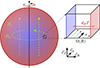 |
Fig. 1. Sketch of the system under study. In the inertial frame, the differentially rotating flow is confined between two shells, subjected to a radial thermal gradient and immersed in a magnetic field with both axial and azimuthal components. |
Here, U is the velocity field, B the magnetic field, P is the pressure, ρ the density, T the temperature, γ the coefficient of thermal expansion, g the gravity, and ν and κ are the kinematic viscosity and thermal diffusivity, respectively.
Furthermore, Eqs. (1) to (4) are perturbed around a background state. Each field is decomposed into a reference component and a perturbation, such that for a given quantity A, we obtain  . We assume that the reference state is characterised by a cylindrical rotation profile, so that U0 = R Ω (R)eϕ and we decompose the magnetic field into axial and toroidal components B0 = Bϕ(R)eϕ + BZ ez. The reference temperature profile T0(R) is assumed to be spherically symmetrical and the induced gravitational disturbances g′ are neglected. Within the Boussinesq framework, the buoyancy term is directly proportional to the temperature perturbation and the background temperature gradient is taken to be positive to represent a stably stratified medium. For the perturbations, we performed a local analysis at the equator, using the Wentzel-Kramers-Brillouin (WKB) approximation following Eckhoff (1981) and Friedlander & Lipton-Lifschitz (2003). Hence, the perturbations were developed as
![Mathematical equation: $$ \begin{aligned} A^\prime = a \, \exp \left[\sigma t + i(k_R R + m \phi + k_Z Z)\right], \, \end{aligned} $$](/articles/aa/full_html/2026/03/aa58545-25/aa58545-25-eq6.gif) (5)
(5)
where a represents the eigenmode’s relative amplitude in the linear regime, m is the azimuthal degree, kR, kZ are the radial and axial wavenumbers, σ is the complex growth rate defined by σ ≡ σr − i(ω + mΩ), with σr the growth rate (if σr > 0) or the decay rate (if σr < 0), ω is the frequency, and mΩ the frequency shift due to the relative motion of the perturbation (analogous to the Doppler effect). In line with the WKB approximation, the quantities associated with the background are considered uniform over the wavelength and curvature terms are neglected so that kR, kZ ≫ 1/R, m/R1. In the following, the wavenumber and its components are scaled by 1/R and the complex growth rate, σ, is scaled by the local rotation frequency, Ω, whilst keeping the same notation for the sake of brevity. The alignment of the mode with the rotation axis is quantified with α = kZ/k, where k is the mode wavenumber. In addition, the background gravity (g0) is considered to be uniform and can be expressed more generally as the Brunt-Väissälä frequency,  .
.
Using Eq. (5) together with the short wavelength approximation for the perturbation into Eqs. (2) to (4) leads to the eigenvalue problem,
 (6)
(6)
where we can use the solenoidal constraints in Eqs. (1) to reduce the system to five independent perturbations. The perturbation vector, V′, is therefore defined as
 (7)
(7)
while the matrix operator, ℋ, is expressed as
 (8)
(8)
where we adopted the notations as described in Table 1.
Dimensionless parameter set (Prandtl, magnetic Prandtl, Ekman, Elsässer, azimuthal Elsässer, stratification, and shear-rate number), with typical values used in DNS and estimates for stellar radiative regions.
The diagonal terms in ℋ correspond to viscous, magnetic, and thermal diffusions, expressed with Ek = ν/ΩR2 and Ekη = Ek/Pm, Ekκ = Ek/Pr. The terms 𝒮B = i(𝒯B, Z + 𝒯B, ϕ), with  and
and  , represent the magnetic stress coupling the velocity and magnetic perturbations. The angular velocity shear is defined as Ro ≡ (R/2Ω)dRΩ and only regimes with Ro < 0 are to be considered. Similarly, the magnetic shear is given by Rb ≡ (R2/2Bϕ)dR(Bϕ/R). The term 2Ro represents the driving source of the magneto-rotational instability, while −2(1 + Ro) represents the source of the hydrodynamic shear instabilities. To avoid any magnetic kink instabilities, our focus was exclusively on the stabilizing effect of magnetic pressure and set Rb = −1. We also note that in the limiting isothermal case where buoyancy effects vanish and the GSF cannot develop, the formulation was reduced to that of Kirillov et al. (2014).
To maintain physical consistency, we imposed a geometric constraint on the admissible modes, such that their wavelengths needed to remain smaller than the characteristic system size (i.e. kRR ≥ 2π and kZR ≥ 2π). This condition is slightly more permissive than the strict requirement for the validity of the WKB approximation. Furthermore, to exclude modes that are strongly damped by viscosity, we required the viscous damping rate to remain smaller than the typical growth rate (i.e. νkR2, νkZ2 ≤ |Ro|Ω; see Sect. 2.2.2). With the numerical method described in Appendix A, we then solve the eigenvalue problem given in Eq. (6) for a set of wavevector. We then retained the mode with the largest growth rate, as it is expected to govern the onset of the instability. This method only allows us to study low azimuthal wavenumber (m ≪ kRR, kZR). Our results can be viewed as indicative of the trends one might expect when extending the analysis to larger values of m. However, such an extrapolation implicitly assumes that curvature and other m-dependent effects remain negligible.
2.2. Magneto-rotational instabilities (MRI)
2.2.1. Validation of the local approach
We present here the SMRI parameter domains using the same representation as Philidet et al. (2020). To do so, we reformulated the eigenvalue problem in terms of adapted dimensionless parameters (see Table 1). The key numbers considered are the Ekman, axial Elsässer, Prandtl, magnetic Prandtl, stratification, and shear numbers, denoted (Ek, ΛZ, Pr, Pm, (N/Ω)2, Ro). For the SMRI, non-axisymmetric perturbations differ from the axisymmetric case only by a frequency shift of +mΩ, so the study is restricted to m = 0. Figure 2 shows the phase diagram of system stability in the (Pm, ΛZ) plane for parameter values typical of DNS and stellar radiative regions.
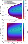 |
Fig. 2. Top panel: Growth rate, σr, normalised by Ω in the (Pm, ΛZ) plane of the axisymmetric SMRI, for a regime typical of DNS. See details in Table 1, with Ro = −0.05, (N/Ω)2 = 1, Λϕ = 0. The three dashed lines correspond respectively to the three criteria Equation (9). The blank region corresponds to the stable parameter domain. The dotted lines correspond to ΛZ, L, ΛZ, U, from the Eq. (12), when ΛZ, U > ΛZ, L. Bottom panel: Growth rate, σr, normalised by Ω in the (Pm, ΛZ) for a regime of radiative stellar region (see Table 1, with Ro = −0.05, (N/Ω)2 = 10, Λϕ = 0). |
The main limits within the phase diagram are well-known (see Chandrasekhar 1960; Acheson & Gibbons 1978; Balbus & Hawley 1991): below a given Pmmin, the instability does not develop. Above that critical value one can also see that the system is only unstable if ΛZ is in a certain window, whose width increases with Pm. The upper bound in terms of ΛZ corresponds to an excessive magnetic strength. The lower bound in terms of ΛZ is imposed by magnetic diffusion. In addition, as shown by Menou et al. (2004) and Philidet et al. (2020), stratification has a stabilizing influence on SMRI modes, setting the threshold value Pmmin that depends on the competition between shear and stratification. Combining these representations, we recovered the three well-known criteria, namely,
![Mathematical equation: $$ \begin{aligned} \begin{aligned} {\left\{ \begin{array}{ll} 4\dfrac{k_Z^2}{k^2} \mathrm{Pm}\left|\mathrm{Ro}\right|< \left(k_Z^2 \Lambda _Z + m^2 \Lambda _\phi \right) \mathrm{Ek},& {\boldsymbol{(i)}} \\ \left|\mathrm{Ro}\right|\left[1+ \left(k_Z^2 \Lambda _Z + m^2 \Lambda _\phi \right) \dfrac{\mathrm{Pm}}{\mathrm{Ek}k^4} \right]< 1+ \dfrac{\mathrm{Pr}}{4}{(\mathrm{N}/ \Omega )^2},& {\boldsymbol{(ii)}} \\ 4 \mathrm{Pm}\left|\mathrm{Ro}\right|< \mathrm{Pr}{(\mathrm{N}/ \Omega )^2}.& {\boldsymbol{(iii)}} \end{array}\right.} \end{aligned} \end{aligned} $$](/articles/aa/full_html/2026/03/aa58545-25/aa58545-25-eq13.gif) (9)
(9)
The limits obtained with our numerical method are in very good agreement with the theoretical criteria. As can be seen by comparing the two panels of Fig. 2, the range of ΛZ values that permits the development of the SMRI is much broader in realistic stellar regimes than in typical DNS regimes. This reflects the fact that diffusive processes are comparatively inefficient in radiative regions, so the window of unstable modes is wider. In Appendix B, we display the stability domain of the same regime parameters towards AMRI2, where the azimuthal Elsässer Λϕ = Bϕ2/(ρμ0Ωη) has to be considered instead of ΛZ. The limit of the unstable parameter domain corresponds also to the limits of Eq. (9).
2.2.2. Growth rates of the MRI
The purpose of this sub-section is to derive general expressions for the growth rates of both SMRI and AMRI to determine the conditions under which an effective MRI can operate. Although these approximate expressions only hold when the perturbations remain small compared to the background quantities, they are useful for estimating which type of instability is likely to dominate and develop efficiently. While non-linear saturations may modify the general dynamics, the expressions we develop next are of interest for implementation in stellar evolution codes since an instability must have a growth time (τr = σr−1) shorter than the typical stellar evolutionary timescale (τevol) to be effective.
Figure 2 shows the growth rate of the SMRI. Our calculation exhibits a plateau within which the instability behaves ideally and approaches its maximum growth rate (σ0), which is equal to |Ro| Ω for |Ro|≤2 and to  otherwise. This plateau is bounded by lower and upper limits on the magnetic field strength,
 (10)
(10)
with Romin defined by Eq. (12). These limits are displayed in Fig. 2 and correspond, respectively, to the magnetic field strengths at which magnetic stress balances either diffusion combined with the Coriolis effect, or magnetic tension competes with stratification to counteract shear. The first limit is consistent with the non-stratified case derived by Petitdemange et al. (2008), while the second extends this framework by identifying a new stabilizing regime arising from the interplay between magnetic tension and buoyancy.
To go further, because this growth rate can serve both to identify the dominant instability in simulations and to estimate the associated angular momentum transport in stellar evolution codes, we propose a simple analytical fit that provides accurate values without solving the full eigenvalue problem across the unstable parameter domain (Eq. (6)). Guided by the numerical growth rates together with Eq. (9), we found that the following expression best reproduces our calculation,
![Mathematical equation: $$ \begin{aligned} \sigma _{\mathrm{SMRI} } \equiv \sigma _0 \left[1+Q^2\left(\dfrac{\Lambda _Z}{\Lambda _{Z,U}} + \dfrac{\Lambda _{Z,L}}{\Lambda _Z}\right) \right]^{-1}, \end{aligned} $$](/articles/aa/full_html/2026/03/aa58545-25/aa58545-25-eq16.gif) (11)
(11)
with
 (12)
(12)
For the regimes shown in Fig. 2 (top and bottom panels), the approximated formula (Eq. (11)) is consistently close to the numerical values of σr, lying between σr and 1.46 × σr. Across all other regimes tested, σSMRI reproduces the numerical growth rates σr fairly well. We also note that for a given flow regime, the maximum growth rate occurs for a magnetic field strength ΛZ, C such that ΛZ, C2 = ΛZ, L × ΛZ, U, as implied by Eq. (11).
For the AMRI (as detailed in Appendix B) the squared growth rate scales as Λϕ/Pm for a given m. Consequently, unlike the SMRI, they do not reach a plateau over a given range of magnetic field strengths. However, as for the SMRI, it is possible to reproduce the numerical growth rates and it is expressed as
 (13)
(13)
with
 (14)
(14)
Equation (13) is consistently close to the numerical result with σr ranging between 0.3σr and 3σr. It deviates significantly from σr only near the boundary of the unstable domain. The simple expression σAMRI further reproduces rather well the numerical values σr across all other regimes tested. Its worth noting that both Eq. (13) and numerical results reach their maximum for Λϕ, U/5 and when |Ro|≫Romin one has σAMRI(Λϕ, C)∼σ0.
Since both Λϕ, L and Λϕ, U depend on m, unstable azimuthal magnetic fields satisfy Λϕ < Λϕ, U(m = 1). Moreover, if an azimuthal wavenumber, m, exists such that m ≪ kRR, kZR and Λϕ ∼ Λϕ, U/5, the characteristic growth time approaches the ideal timescale, τr ∼ τ0. This result agrees with the local prediction from the local linear theory of Masada et al. (2006). For weaker magnetic fields, high m values that fall outside the strict validity of the local approximation are required; this point is discussed in Sect. 4.
Figure 3 shows that the approximated expressions of the growth rate (Eqs. (11) and (13)) reliably reproduce the instability timescales across different magnetic configurations. With respect to the helical magnetic field, for ΛZ < ΛZ, C, the SMRI and AMRI form distinct branches and the fastest mode dominates; when they become simultaneously competitive, a reinforced hybrid mode may occur. For stronger axial fields (ΛZ > ΛZ, C), the AMRI is suppressed and only the SMRI remains, while sufficiently large azimuthal magnetic stress (Λϕ > Λϕ, max) stabilises the SMRI itself. Overall, our findings show an excellent agreement with the linear analysis of SMRI and AMRI reported in Petitdemange et al. (2013) and further extend this framework by incorporating stabilising thermal stratification. Finally, we note that in the parameter regimes explored here, we did not recover the helical MRI branch described by Liu et al. (2006) and Kirillov et al. (2014)3. Instead, we found only a helically modified MRI, which differs only slightly from the SMRI or AMRI. For this reason, we did not pursue the study of the helical MRI further in the context of radiative stellar interiors. In Appendix B, we provide additional details on the mode structure of the SMRI and AMRI and give local prescriptions for the radial and vertical scales of the unstable modes.
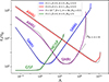 |
Fig. 3. Growth time, τr/τΩ (=Ω/σr), as a function of Λ for different magnetic-field configurations, parametrised by ΛZ = δ2Λ, Λϕ = β2Λ. We consider regimes representative of stellar radiative zones (Table 1): a weakly stratified, low-shear case (|Ro| = 0.5, (N/Ω)2 = 1) relevant to the MRI, and a strongly stratified, high-shear case (|Ro| = 5, (N/Ω)2 = 5 × 10³) relevant to the GSF and MGSF instability (Sect. 3). The dotted lines show the analytical growth rate estimates (Eqs. (11), (13), and (17)). |
3. Magnetised GSF (MGSF) instability
3.1. Transition from SMRI to GSF
We first considered the transition from SMRI to GSF in flows where the magnetic field is too weak to significantly modify the unstable domain. This allows us to identify how magnetic fields alter the properties of the instabilities and how, together with the effect of stratification, SMRI modes can smoothly transition into magnetised GSF (MGSF) modes.
In Fig. 4 (top panel), the phase diagram (|Ro|,(N/Ω)2) is displayed for a sheared flow in a regime typical of radiative regions (see Table 1) with ΛZ = 100. The dashed lines show the boundary between the stable and unstable domains for each instability4. The SH modes correspond to large scales (small k), SMRI to intermediate scales, and MGSF to smaller scales. For sufficiently strong magnetic fields, SMRI modes (SMRI∥) remain aligned with the field, whereas MGSF modes become nearly perpendicular, reflecting the balance between shear destabilisation and magnetic stabilisation. As shown in Fig. 4 (bottom panel), weak stratification produces a broad SMRI-dominated unstable range, while stronger stratification narrows this range and shifts the orientation of the most unstable mode. Since the transition from SMRI to MGSF is continuous in the (k, kZ/k) plane, the modes evolve smoothly between the two, passing through SMRI-like modes that become nearly perpendicular to the rotation and magnetic-field axes (SMRI⊥). This gradual re-orientation resembles the behaviour reported by Dymott et al. (2024), who showed that magnetic fields tilt the GSF-unstable domain and produce SMRI modes aligned with the angular momentum gradient.
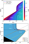 |
Fig. 4. Top panel: Growth rate σr/Ω in the (|Ro|,(N/Ω)2) of the SMRI, GSF and SH instabilities, for a regime typical of radiative regions (see Table 1, ΛZ = 100, Λϕ = 0). The three dashed lines correspond to instability thresholds, red for SMRI (Eq. (9)), blue for GSF, green for SH. The dotted lines separate the dominant type of instability inside the unstable domain from the mode properties. Bottom Panel: Stability map in the (k, α) plane for a stellar regime with |Ro| = 3 and ΛZ = 100. Solid colored curves show the boundaries of the unstable domains for several values of the stratification parameter (N/Ω)2. The blue region corresponds to the unstable range for (N/Ω)2 = 10, and the star markers indicate, for each (N/Ω)2, the most unstable mode (corresponding to the regimes indicated by the stars in the top panel). The black region denotes modes excluded by our assumptions. The densely dashed horizontal line indicates the upper limit of the GSF-unstable domain set by magnetic stresses. The dashed lines show the modified stability boundaries due to the combined action of magnetic stresses and stratification, shown here for (N/Ω)2 = 5 × 10³ and 5 × 10⁵. The loosely dashed line marks the limit imposed by viscous diffusion. Labels indicate the domains of SMRI‖, SMRI⊥, and MGSF modes. |
Once stratification stabilises the SMRI, the MGSF domain is limited by resistive effects that impose an upper limit. In addition, the magnetic stress restrict the mode orientation, the viscous effects damp small-scale modes, and the magneto-stratification excludes large-scale modes. These properties of the MGSF domain and mode properties are quantified and detailed in Appendix C.1.
3.2. Magnetised GSF: Stability criterion
While some stellar models appear compatible with the development of GSF modes (e.g. Fellay et al. 2021), recent studies have shown that magnetic fields can strongly damp these modes (Caleo et al. 2016; Dymott et al. 2024). Because these results were obtained in specific parameter regimes, our goal is now to derive general stability criteria that explicitly account for the stabilizing effect of an axial magnetic field, thereby allowing us to assess the occurrence of GSF modes in a more realistic stellar context.
To this end, following the approach used to determine the unstable mode range, we used the marginal stability equation to examine two regimes. Compared with the standard criterion, we incorporated additional stabilizing forces and by focussing on the most unstable mode, we were able to derive new conditions. We first considered a regime in which the additional stabilizing forces are due to mixed diffusion and magnetic stress. By identifying the mode (k, kZ/k) that minimises stabilisation, we obtained a first correction term (hereafter, 𝒞1, defined in Eq. (16)) to the stability criterion. Second, we add the stabilizing forces due to viscous diffusion and the magneto-stratification interplay. In this case, in a similar way, we obtained a second correction term (hereafter, 𝒞2, defined in Eq. (16)). The detailed derivation (described in Appendix C) finally gives a sufficient MGSF stability criterion of
 (15)
(15)
where
![Mathematical equation: $$ \begin{aligned} \mathcal{C} _1&= 2 \sqrt{2} k_{Z,\mathrm{min}} \Lambda _Z^{3/2} \mathrm{Ek}^{1/2}, \nonumber \\ \mathcal{C} _2&= \dfrac{5}{2}\left(\dfrac{2}{3}\right)^{3/5} \left(k_{Z,\mathrm{min}}^2\mathrm{Ek}\Lambda _Z^3 \mathrm{Pr}^3 \left[{(\mathrm{N}/ \Omega )^2}- 4 \mathrm{Pm}\vert \mathrm{Ro}\vert /\mathrm{Pr}\right]^3 \right)^{1/5}. \end{aligned} $$](/articles/aa/full_html/2026/03/aa58545-25/aa58545-25-eq21.gif) (16)
(16)
The mode kZ, min designates the mode with the largest axial extent allowed within the domain and, therefore, the non-dimensional vertical wavenumber is expressed as kZ, min = 2π. In Fig. 5, the phase diagram (|Ro|,(N/Ω)2) of a stellar regime with a strong magnetic field (ΛZ = 105) is displayed. The limits of the unstable domain are well reproduced by the criteria of the SMRI at low shear values and MGSF at stronger shear values. The expressions of the MGSF criterion (Eq. (15)) capture the limits of the unstable parameter domain.
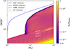 |
Fig. 5. Ratio of the growth rate σr to the analytical formula σestim ≡ max(σSMRI, σMGSF), which combines the predictions for SMRI (Eq. (11)) and MGSF (Eq. (17)). The flow parameters correspond to those of Fig. 4 (top panel), with ΛZ = 105. The white dotted lines delimit the different instability domains (see Appendix C and Fig. C.1 for details). The black dashed line indicate the sufficient MGSF stability criterion (Eq. (15)). The grey dotted line correspond to the combination of the necessary criteria (Eq. (C.12)). See Appendix C.3 for details. |
While the first corrective term, 𝒞1, shifts the minimum shear required for instability, the second term, 𝒞2, introduces additional stabilisation, particularly at low stratification and shear. This behaviour also holds in more viscous regimes, such as those corresponding to the DNS parameters listed in Table 1. When the corrective terms 𝒞1 and 𝒞2 are omitted, the standard GSF criterion is recovered.
The criterion derived in this section can be used to assess the relevance of the MGSF instability in stellar interiors when the poloidal component of the magnetic field is known or can be reasonably estimated. A non-zero axial magnetic field (ΛZ ≠ 0) tends to stabilise configurations that would otherwise be unstable (as noted by Caleo et al. 2016; Caleo & Balbus 2016; Dymott et al. 2024).
3.3. Magnetised GSF: Growth rate
To go further, we aim to derive a simple estimate of the growth rate of the magnetised GSF instability, enabling an assessment of its efficiency in radiative stellar regions. Considering regimes that are GSF-unstable but MRI-stable, we examine how the GSF growth rate varies with the flow parameters. As in the previous section, we find an approximate formula given by
 (17)
(17)
where
 (18)
(18)
We note that in Eq. (17), the first prefactor is mainly relevant for regimes close to the marginal stability, whereas the second reflects the general magnetic slowing.
We illustrate the validity of this analytical formula in Figs. 3 and 5, where we introduce σestim ≡ max(σSMRI, σMGSF). Across the unstable parameter domain, σestim remain very close to the numerical results σr, supporting the validity of our formula in strongly magnetised flows. In the middle of the transition region, however, σestim tends to underestimate σr because it only accounts for the maximum of SMRI and MGSF, whereas both instabilities can act simultaneously. Moreover, near and below the SH criterion, the additional instability is not considered when it converges more closely to σ0.
The analytical formula (Eq. (17)) is consistent with the simulations of Caleo & Balbus (2016), which show that the damping time of transient modes in a magnetised background is inversely proportional to the magnetic resistivity. The local analysis of Dymott et al. (2024) likewise highlights the role of Ohmic dissipation in weakening magnetic stabilisation. To illustrate the need for this criterion, we consider the case of the Kepler 56 target: using the results of Fellay et al. (2021) together with a magnetic diffusivity η = η⊙ (as in Caleo & Balbus 2016), we obtained a very low stabilizing threshold for the magnetic field, BMGSF ∼ 5G. This underscores the importance of accounting for magnetic stabilisation when modelling GSF modes in stars, particularly in stellar evolution models that include GSF-driven angular momentum transport.
4. Global approach
4.1. Methodology
We now consider a flow between two differentially rotating cylinders, at a radius of Rin, Rout = 2Rin having different angular velocities, Ωin, Ωout, and temperature, Tin, Tout, immersed in a magnetic field, B = BZeZ + Bϕ,in(Rin/R)eϕ. This problem is the magnetohydrodynamic, radially stratified version of the Taylor-Couette system. Such a configuration allows us to emphasise the effects of azimuthal curvature and radial boundary conditions and it is particularly suited to studying instabilities with short axial wavelengths (large kZ), which are comparatively less sensitive to latitudinal curvature.
We extended the non-stratified linear stability code going back to Hollerbach & Rüdiger (2005), Hollerbach et al. (2010), Child et al. (2015); we implemented a new temperature equation and radial temperature gradient as described in Appendix. D. Then we chose to focus on modes that are confined within the bulk of the domain, excluding those that develop primarily near the inner or outer boundaries. To ensure this, we applied no-slip boundary conditions for the perturbed velocity field U′, perfectly conducting boundaries for the magnetic field B′, and fixed-temperature conditions for T′ (see Appendix D.1). We assume perturbations to be of the form A′=a(R)exp[σt + i(mϕ + kZZ)]. We note that due to the large size of the matrix, (5Nrp + 12)2 with Nrp ∈ [30, 60], only viscous and weakly stratified regimes can be numerically solved.
4.2. Global MRI modes
4.2.1. MRI: Unstable parameter domain and growth rates
We first examined the conditions under which the SMRI arises in the (Pm, ΛZ) plane, focussing on the flow regimes shown in Fig. 6 (top panel). The unstable parameter domain closely matches the predictions of the local criterion (Eq. (9)) and the growth rates, σr, agree well with the analytical expression, σSMRI (Eq. (11)), throughout the unstable region of Fig. 6 (top panel). We also find a similarly good agreement for the axial wavenumbers, kZ, of the modes, yielding remarkably consistent mode properties between the local and global analyses.
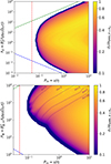 |
Fig. 6. Top panel: Ratio σr/σSMRI, R = Rin in the (Pm, ΛZ) plane of the SMRI for regimes with Pr = 10−3, Ek = 10−5, Ro = −0.5, (N/Ω)2 = 102. The estimate σSMRI, R = Rin comes from the local model Eq. (11) evaluated at R = Rin and σr corresponds to the numerical values obtained with the global code. The green, red and blue dashed lines correspond to the criteria introduced in the local approach (Eq. (9)). Bottom panel: Ratio σr/σAMRI, R = Rin in the (Pm, Λϕ) plane of the Azimuthal MRI for the same regime than top panel and considering the fastest mode among the set of azimuthal wavenumbers m ∈ [1, 2, 5, 7, 10] and σAMRI, r = Rin from Eq. (13). The blue and green dashed lines corresponds to the criteria for m = 1 (Eq. (9)). The dashed lines indicate the parameter region in which a given azimuthal mode number, m, yields the maximum growth rate. |
We then considered the AMRI in Fig. 6 (bottom panel) and examined the stability of regimes in the (Pm, Λϕ) plane for modes with m ∈ [1, 2, 5, 7, 10]. The expected scaling relations for thermal stratification and for the resistive limit were successfully recovered. However, the diffusive limit (Eq. (9)ii) departs significantly from the local prediction: in Fig. 6 (bottom panel), Λϕ, min remains two orders of magnitude above the local estimate for m = 1, and roughly four orders of magnitude above the local m = 10 estimate (not shown). At low azimuthal wavenumber, Λϕ, min is almost independent of the diffusive ratio, Pm = ν/η, in agreement with previous studies (Rüdiger et al. 2010, 2015). We ruled out the variation of local background parameters as the origin of this discrepancy and find instead that the intrinsic non-axisymmetry of AMRI modes (e.g. curvature and azimuthal-drift effects) provides an additional stabilizing influence that is absent from the local WKB analysis (for the low Pm limit, see Rüdiger et al. 2014). This could also explain why AMRI is more sensitive to global properties than SMRI. Whether this difference remains significant under stellar conditions is left for future investigation. However, within the unstable domain the growth rates σr remain close to σAMRI, except near the stability boundaries where additional non-local stabilizing effects become important. Overall, our results indicate that locally derived unstable domains and mode characteristics remain applicable to global SMRI and AMRI configurations, except in the regime of weak azimuthal fields, where additional stabilizing forces become significant.
4.2.2. MRI: Mode location
Beyond determining whether modes are unstable, it is crucial to predict where they preferentially develop within the flow. In stars, this identifies the regions that most efficiently transport angular momentum, mix elements, or amplify magnetic fields.
We first examined the location of SMRI modes between the two differentially rotating cylinders. Fixing the boundary temperatures and angular velocities through the diffusive equilibrium constrains the background profiles. Thus, we adopted the thermal stratification N2(R) = NR = Rin2(Rin/R)4 ad hoc to test cases with steep stratification. Figure 7 shows the radial velocity perturbations for different stratification strengths. The most unstable modes emerge at different radii, depending on the combined effect of shear and rotation, and they consistently localise where the analytical formula (red curves) peaks. The axial wavenumbers are slightly smaller than local estimates (see Table D.2). Finally, the radial extent of the modes is non-negligible, owing to diffusion, boundary effects, and the radial variation of the flow parameters, which sharpens the local growth rate profile.
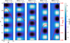 |
Fig. 7. Reconstructed radial velocity perturbations U′R(R, Z) of the most unstable eigenmode in regimes with ΛZ = 1.6, Ek = 10−5, Pm = 1, Pr = 0.1, at R = Rin and stratification amplitudes (N/Ω)2R = R∈in of 1, 1.3, 1.5, 2, and 2.5. The maximal shear is |Romax| = 0.05. The corresponding growth rate computed is given below the stratification value considered. The red overlayed curves correspond to the analytical formula (Eq. (11)). The vertical black dashed lines give the radius where the mode amplitude peaks and the vertical red dashed lines give the radius where the analytical formula reaches its maximum. |
Across different regimes and profiles studied, we find that the analytical formula of the SMRI growth rate (Eq. (11)) also predicts the radial position of unstable SMRI modes. The numerical results for σr lie between σSMRI and 1.14 × σSMRI, confirming the reliability of the local prediction. For the AMRI, the agreement remains satisfactory in several regimes, although curvature and boundary effects influence the instability location in some extreme parameter regimes. Additional configurations explored are presented in Appendix D.2. While future works would need to validate this result with 3D global simulations, we conclude that taking the growth rates as estimated by local analysis constitutes a valuable proxy for estimating the location where the instability preferentially develops within the flow.
4.3. MGSF in a Taylor-Couette geometry
Finally, we investigated the MGSF. The strong differential rotation required by this instability leads to large radial variations of Ω(R), which would induce spatial variations of the local dimensionless numbers. To retained a homogeneous force balance, we therefore prescribed constant values of (Ro, (N/Ω)2, ΛZ, Ek) throughout the domain, adjusting the coefficients so that the local parameters remain fixed. This choice isolates the role of magnetic stabilisation.
Figure 8 shows the phase diagram in the (Λ, Ek) plane for a flow configuration that is unstable to the GSF but stable to the MRI. Although numerical constraints limit our ability to explore stronger magnetic fields, the boundary of the unstable region agrees well with the extended criterion in Eq. (15), which includes magnetic stabilisation. The eigenvalue problem is computationally demanding and sensitive to spurious modes: resolving GSF (and especially MGSF) modes requires fine radial discretisation5 to obtain converged growth rates consistent with the local estimate (Eq. (17)). However, increasing the resolution also reduces the numerical stability of the solver (see Appendix D.3 for details). Despite these numerical challenges, the stabilising influence of magnetic fields is clearly reproduced: magnetic tension reduces the growth rate in accordance with the predicted scaling. Compared with the standard GSF, magnetised regimes involve smaller radial length scales, further reinforcing the need for high spatial resolution to accurately resolve MGSF modes.
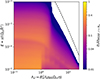 |
Fig. 8. Ratio σr/σMGSF, R = Rin in the (ΛZ, Ek) plane for the MGSF, with Pm = 0.1, Pr = 10−2, Ro = −6, (N/Ω)2 = 400, and Λϕ = 0 and the resolution, Nrp = 30. Shear and stratification are constant across the domain, as are the Elsässer and Ekman numbers. The green dashed line marks the MGSF stability criterion (Eq. (15)). |
The global Taylor-Couette analysis confirms the validity of the local approach. For the SMRI, both the stability thresholds and the growth rate estimates agree very well with the global results and they correctly predict the radial localisation of unstable modes across the domain. For the AMRI, some discrepancies appear in the weak-field regime, but the local estimates remain accurate throughout the unstable parameter domain. Finally, extending the analysis to strongly sheared flows shows that magnetic fields can effectively stabilise GSF modes.
5. Application to low-mass subgiants and young red giants
We applied our analysis to stellar conditions representative of low-mass subgiants and young red giants. These evolutionary stages are particularly interesting because asteroseismic observations provide estimates of both core and envelope rotation rates (Deheuvels et al. 2014, hereafter D14). Thus, our aim has been to determine whether fields comparable to those observed in red giant cores (for a review, see Deheuvels 2024) could give rise to shear-driven instabilities. We considered two stars from sample of D14 (denoted as A and F; see also Table 2).
Input parameters and surface properties of the stellar models of stars A and F in the D14 stellar sample, computed with the newest version of Cesam2k20.
5.1. Stellar evolution models
The stellar structure models used for this work were computed with the Cesam2k20 6 stellar evolution code (Morel 1997; Morel & Lebreton 2008; Marques et al. 2013; Manchon et al. 2025). The physical ingredients were chosen to be as close as possible to the one used by D14. Present models use Grevesse & Noels (1993)’s determination of the solar chemical composition, with opacity tables from the OPAL team (Rogers & Iglesias 1992; Iglesias & Rogers 1996), adapted to these abundances. The tables are supplemented, for low temperature values, by the Wichita7 opacity tables (Ferguson et al. 2005). We note here that the chemical composition used by D14 to generate the opacity tables might be slightly different. The equation of state (EoS) uses data from the tables published as part of the OPAL 2005 EoS (Rogers & Nayfonov 2002). The nuclear reaction rates follow the compilations from NACRE (Aikawa et al. 2006), apart from LUNA (Broggini et al. 2018) for the 14N(p, γ)15O reaction. The convection is modelled with the full turbulent spectrum formalism of Canuto et al. (1996). The atmosphere was retrieved using the Eddington T(τ) relation. The effects of overshoot and rotation were not considered.
To recover observational parameters within uncertainties given by D14, we had to slightly adjust the input parameter of each model, within the range of values they considered for their grid-based approach. This is due to the different version of the code, small differences in the input physics, and round-off errors in the value of the input parameters provided in D14. These parameters are gathered in Table 2. From the models, the profiles of Prandtl, Pr = ν/κ, and magnetic Prandtl, Pm = ν/η, numbers have been extracted, where ν is the kinematic viscosity, η the molecular magnetic diffusivity, and κ the thermal diffusivity, following the formulations of Spitzer (1962), Mihalas & Mihalas (1984).
5.2. Rotation and magnetic field models
Asteroseimic observations provide estimates of mean core and surface rotation so that the exact profile is not accurately know. Therefore, based on the core and envelope rotation-rate estimates given in D14, we constructed two types of models, which we then tested. A smooth one as proposed by D14,
 (19)
(19)
with r★ the radius of the radiative-convective transition and a sharper one assuming a strong decrease of angular velocity (see also Belkacem et al. 2015) set with
 (20)
(20)
where m is the local mass, md defines the mass where the angular velocity drops, and wd controls the width of the transition.
For the magnetic field, several estimates of the core magnetic field of red giants have been debated (e.g. Fuller et al. 2015; Mosser et al. 2017; Li et al. 2022; Deheuvels et al. 2023). For some of them, strong radial fields of the order of 100 kG have been detected near the hydrogen-burning shell. In the following, we assume a poloidal magnetic field dominated by a dipolar component, such that the axial and the radial field components are of the same order, BZ ∼ Br. We consider the axial component at the equator of the magnetic field generated by a dipole, expressed as
 (21)
(21)
where BZ, 0 is the axial field value at the radius, rb, where the Brunt-Väissälä frequency reaches its maximum. This approach allows us to use instabilities onset properties expressed in terms of BZ, 0, while discussing the astrophysical case, where only the radial field Br is observationally constrained near the hydrogen-burning shell. The case of an azimuthal or toroidal magnetic field will be addressed in a forthcoming study, where (in addition to the AMRI) magnetic kink-type instabilities such as the Tayler instability (TI) are expected to play a role.
Then, we can solve Eq. (6), using the local background values at each radius to determine the instability domains predicted by our local approach. For all models tested, we found that the SMRI and MGSF criteria (Eqs. (9) and (15)), together with the corresponding analytical expressions for their growth rates (Eqs. (11) and (17)), successfully identify the unstable regions and accurately characterise their properties. We emphasise that these semi-analytical formulas (Eq. (22)) reliably predict both the existence and the timescales of the instabilities at very low computational cost (without the need to solve Eq. (6)) and can therefore be implemented directly in stellar evolution codes. When the regime is unstable, the corresponding growing times are expressed as
![Mathematical equation: $$ \begin{aligned} \tau _{\mathrm{SMRI} }&\equiv \tau _0 \left[1+Q^2\left(\dfrac{\Lambda _Z}{\Lambda _{Z,U}} + \dfrac{\Lambda _{Z,L}}{\Lambda _Z}\right) \right], \nonumber \\ \tau _{\mathrm{MGSF} }&\equiv \tau _0 \left(1+ \dfrac{2 \Lambda _Z}{\sqrt{\vert \mathrm{Ro}\vert -1}}\right) \left( \dfrac{1+2\sqrt{\vert \mathrm{Ro}\vert } \mathcal{B} }{\left(1-\mathcal{C} \right)^{3/4}} \right), \end{aligned} $$](/articles/aa/full_html/2026/03/aa58545-25/aa58545-25-eq27.gif) (22)
(22)
with τ0, Q, ΛZ, L, ΛZ, U, ℬ, 𝒞 as presented in Sects. 2 and 3. black
5.3. Results
For evolved low-mass stars, structural evolution is essentially driven by the core contraction with a typical timescale, denoted as  . The spatial mean of this characteristic timescale is found for stars A and F to be,
  and
and  respectively. Comparing the instability growth times with this characteristic timescale provides a measure of whether (and to what extent) these instabilities can develop during the stellar evolution phase.
Star A: In Fig. 9 (left panels), we present the results for Star A. The top panel corresponds to a sharp rotation profile and a moderate magnetic field (BZ, r = rb = 1 kG), showing the development of the MGSF. For stronger fields, magnetic stabilisation progressively suppresses the MGSF, leaving the SMRI as the dominant instability, while for weaker fields the GSF prevails8. When a strong magnetic field is considered (BZ, r = rb = 100 kG), the growth time is  , suggesting that the SMRI could develop within the thin shear region. For the model with a linear rotation profile (bottom panel), only the SMRI remains unstable and only in the outer layers where stratification is relatively weak. In this case, the shear lies in a weakly magnetised region, even when assuming a strong field of BZ, r = rb = 100 kG in the hydrogen-burning shell. Consequently, the growth time decreases when going from BZ, r = rb = 1 G to 100 kG, reaching τr ∼ 149 yr in the upper radiative layers and rising sharply with depth. From the other models tested and summarised in Table D.1 (Appendix E), we conclude that for the subgiant Star A, the development of a shear-driven instability requires the shear region to be both narrow enough to sustain a strong rotational gradient and located sufficiently far from the hydrogen-burning shell to mitigate thermal and magnetic stabilisation.
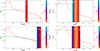 |
Fig. 9. Growth rates of unstable regions for different rotation and Brunt-Väisälä (BV) frequency profiles, shown in the background color scale, are displayed for the stars considered. The type of shear-driven instability (e.g. SMRI, MGSF) is indicated in each panel. The BV profile exhibits a narrow peak corresponding to the hydrogen-burning shell. Its position defines the reference radius, rb. The reference width, wb, is defined as the radial distance over which the BV frequency decreases by an order of magnitude from its maximum at rb. Left panels: Star A, top:BZ, 0 = 1 kG, wd = wb, rd = 5rb. Bottom:BZ, 0 = 100 kG, linear rotation profile Ω(r). Right panels: Star F, top:BZ, 0 = 1 G, wd = 3wb, rd = 2rb. Bottom:BZ, 0 = 100 kG, wd = 5wb, rd = 2rb. |
Star F: In Fig. 9 (right panels), we present the result for Star F. This more evolved star exhibits a larger rotation contrast, Ωin/Ωout, implying stronger shear and a flow more prone to shear-driven instabilities. In the top panel, we consider a sharp rotation profile and a weak magnetic field (BZ, r = rb = 1 G). In the bottom panel, we adopted a smoother profile with a stronger field (BZ, r = rb = 100 kG). For the sharp profile, both SMRI and GSF can develop in distinct regions, with the GSF growing on the fastest timescale, τr ∼ 20 h. When the magnetic field exceeds 1 kG, however, only the SMRI persists, and its growth rate decreases significantly. With the smoother rotation profile and BZ, r = rb = 100 kG, our analysis predicts SMRI growth on a timescale of τr ∼ 31.8 yr. Shear regions located closer to the hydrogen-burning shell experience stronger stabilisation from stratification and magnetic tension, reducing their susceptibility to instability. Conversely, shear zones further from this shell are less stabilised, favouring the growth of shear-driven modes. This again explains why smoother (linear) rotation profiles are particularly prone to fast-growing instabilities in their outer radiative regions.
Overall, if a strong large-scale poloidal magnetic field of the order 100 kG is present in the hydrogen-burning shell of a low-mass subgiant or young red giant (as observed in some red giants) shear-driven instabilities can develop efficiently only if the shear region lies sufficiently far from that shell. Interestingly, for all tested models, the instabilities found have a growth time much lower than the expansion timescale. Additionally, we found only SMRI modes and no GSF or MGSF, when BZ, r = rb ≥ 1 kG.
Although the degree of differential rotation can vary during the post-main sequence evolution, it generally becomes stronger in the early red giant phase for the models considered here. Consequently, shear-driven instabilities are expected to grow more rapidly in young red giants than in sub-giants. For the different rotation and magnetic field configurations tested, we found growth times ranging from a few months to several hundred thousand years, highlighting the need to account for magnetic and stratification effects when assessing the role of shear-driven instabilities in stellar evolution. The simple estimates proposed here can be implemented in 1D stellar evolution codes to evaluate, for instance, the efficiency of angular momentum transport by SMRI through an effective viscosity, νSMRI = σSMRIR2, where the instability develops at radius, R, with a growth rate of σSMRI (similarly to Wheeler et al. 2015; Griffiths et al. 2022). Since GSF and MGSF modes are found to be nearly perpendicular, transport prescriptions derived from previous studies of the GSF instability (e.g. Barker et al. 2019) might not be directly applicable in the magnetic case. While our linear results may provide qualitative guidance on the influence of magnetic fields, dedicated non-linear simulations with a sufficiently fine mesh would be required to establish a saturation theory for the MGSF and, in turn, a reliable model for the associated angular momentum transport.
6. Conclusion
We investigated shear-driven instabilities in stellar radiative regions through a linear stability analysis of MRI and GSF modes. Using a WKB approach, we first derived general estimates for the local unstable modes, then extended the analysis to global Taylor-Couette configurations to assess how these modes arise in finite domains. Finally, we applied our results to stellar models of subgiants and young red giants.
For the SMRI and AMRI, we recovered already known stability criteria and quantified the influence of stratification, magnetic tension, and diffusion on growth rates. In strongly sheared regimes, we derived a new criterion for the magnetised GSF (MGSF) instability and estimated how magnetic and stratification effects reduce the range of unstable modes, clarifying the transition between SMRI and MGSF.
In addition, we derived approximate formulae for the instability growth times, making it possible to determine which instability (i.e. SMRI or MGSF) is likely to dominate under given stellar conditions. Implementing these formulae in 1D stellar evolution codes, through the effective viscosity associated with these instabilities, would enable a more realistic estimation of angular momentum transport throughout stellar evolution. Our results were further validated through stability analyses of Taylor-Couette flows. The global modes confirm that the local WKB framework accurately identifies where instabilities develop and provides reliable estimates of their behaviour across the domain. This strengthens the applicability of the local results to realistic stellar profiles.
When applied to sub-giants and young red giants, our analysis shows that shear-driven instabilities can grow on short timescales for magnetic fields well below 100 kG, suggesting that these mechanisms may readily operate in such stars. Depending on the magnitude and radial location of the shear, our analytical formulae predict where SMRI or MGSF modes should arise within the radiative zone. In contrast, strong axial magnetic fields of order ∼100 kG confined to the hydrogen-burning shell can co-exist with shear-driven instabilities only if the shear layer lies sufficiently far from the shell; in such cases, magnetic tension and stratification act together to suppress most unstable modes. Overall, these results motivate incorporating our instability criteria and growth rate estimates into 1D stellar evolution models to evaluate the role and efficiency of shear-driven instabilities throughout stellar evolution.
A follow-up paper will address magnetically driven instabilities, focussing on Tayler-like modes (Tayler 1973; Spruit 1999; Skoutnev & Beloborodov 2024), thereby complementing recent work on Tayler dynamos (e.g. Petitdemange et al. 2023; Meduri et al. 2025) demonstrating efficient angular momentum transport. The interplay between the MRI, MGSF and Tayler instabilities and, more generally, the potential co-existence of multiple instabilities across different spatial or temporal scales remain an open question (Jouve et al. 2020; Chang & Garaud 2021; Meduri et al. 2024). In addition, the present approach primarily describes the linear onset of the instabilities and cannot independently constrain their non-linear saturation or the associated angular momentum transport, which will be further addressed in future non-linear simulations.
Acknowledgments
The authors thank Oleg Kirillov and Jordan Philidet for useful discussions that helped clarify the work presented, and the anonymous referee for their relevant remarks. They also acknowledge financial support from the “Initiative Physique des Infinis” (IPI), Sorbonne Université, and the “Action Thématique de Physique Stellaire” (ATPS).
References
- Acheson, D. J., & Gibbons, M. P. 1978, Philos. Trans. R. Soc. Lond. Ser. A, 289, 459 [Google Scholar]
- Aerts, C., Mathis, S., & Rogers, T. M. 2019, ARA&A, 57, 35 [Google Scholar]
- Aikawa, M., Arai, K., Arnould, M., Takahashi, K., & Utsunomiya, H. 2006, AIP Conf. Ser., 831, 26 [Google Scholar]
- Aurière, M., Wade, G. A., Silvester, J., et al. 2007, A&A, 475, 1053 [NASA ADS] [CrossRef] [EDP Sciences] [Google Scholar]
- Balbus, S. A., & Hawley, J. F. 1991, ApJ, 376, 214 [Google Scholar]
- Barker, A. J., Jones, C. A., & Tobias, S. M. 2019, MNRAS, 487, 1777 [Google Scholar]
- Belkacem, K., Marques, J. P., Goupil, M. J., et al. 2015, A&A, 579, A31 [NASA ADS] [CrossRef] [EDP Sciences] [Google Scholar]
- Braithwaite, J., & Spruit, H. C. 2017, R. Soc. Open Sci., 4, 160271 [Google Scholar]
- Broggini, C., Bemmerer, D., Caciolli, A., & Trezzi, D. 2018, Prog. Part. Nucl. Phys., 98, 55 [CrossRef] [Google Scholar]
- Caleo, A., & Balbus, S. A. 2016, MNRAS, 457, 1711 [Google Scholar]
- Caleo, A., Balbus, S. A., & Tognelli, E. 2016, MNRAS, 460, 338 [NASA ADS] [CrossRef] [Google Scholar]
- Cantiello, M., Mankovich, C., Bildsten, L., Christensen-Dalsgaard, J., & Paxton, B. 2014, ApJ, 788, 93 [Google Scholar]
- Canuto, V. M., Goldman, I., & Mazzitelli, I. 1996, ApJ, 473, 550 [NASA ADS] [CrossRef] [Google Scholar]
- Chandrasekhar, S. 1960, PNAS, 46, 253 [NASA ADS] [CrossRef] [Google Scholar]
- Chang, E., & Garaud, P. 2021, MNRAS, 506, 4914 [Google Scholar]
- Child, A., Kersalé, E., & Hollerbach, R. 2015, Phys. Rev. E, 92, 033011 [Google Scholar]
- Daniel, F., Petitdemange, L., & Gissinger, C. 2023, Phys. Rev. Fluids, 8, 123701 [NASA ADS] [CrossRef] [Google Scholar]
- Deheuvels, S. 2024, 8th TESS/15th Kepler Asteroseismic Science Consortium Workshop, 116 [Google Scholar]
- Deheuvels, S., Doğan, G., Goupil, M. J., et al. 2014, A&A, 564, A27 [NASA ADS] [CrossRef] [EDP Sciences] [Google Scholar]
- Deheuvels, S., Li, G., Ballot, J., & Lignières, F. 2023, A&A, 670, L16 [NASA ADS] [CrossRef] [EDP Sciences] [Google Scholar]
- Di Mauro, M. P., Ventura, R., Cardini, D., et al. 2016, ApJ, 817, 65 [NASA ADS] [CrossRef] [Google Scholar]
- Durand, E. 1960, Solutions numériques des équations algébriques. Tome I. Équations du type F(x) = 0, racines d’un polynôme (Paris: Masson) [Google Scholar]
- Dymott, R. W., Barker, A. J., Jones, C. A., & Tobias, S. M. 2024, MNRAS, 535, 322 [Google Scholar]
- Eckhoff, K. S. 1981, J. Differ. Equations, 40, 94 [Google Scholar]
- Eggenberger, P., Buldgen, G., & Salmon, S. J. A. J. 2019, A&A, 626, L1 [NASA ADS] [CrossRef] [EDP Sciences] [Google Scholar]
- Fellay, L., Buldgen, G., Eggenberger, P., et al. 2021, A&A, 654, A133 [NASA ADS] [CrossRef] [EDP Sciences] [Google Scholar]
- Ferguson, J. W., Alexander, D. R., Allard, F., et al. 2005, ApJ, 623, 585 [Google Scholar]
- Fricke, K. 1968, Z. Astrophys., 68, 317 [NASA ADS] [Google Scholar]
- Friedlander, S., & Lipton-Lifschitz, A. 2003, Elsevier Press, 2, 289 [Google Scholar]
- Fuller, J., Cantiello, M., Stello, D., Garcia, R. A., & Bildsten, L. 2015, Science, 350, 423 [Google Scholar]
- Fuller, J., Piro, A. L., & Jermyn, A. S. 2019, MNRAS, 485, 3661 [NASA ADS] [Google Scholar]
- García, R. A., Turck-Chièze, S., Jiménez-Reyes, S. J., et al. 2007, Science, 316, 1591 [Google Scholar]
- Goldreich, P., & Schubert, G. 1967, ApJ, 150, 571 [Google Scholar]
- Gough, D. O. 2015, Space Sci. Rev., 196, 15 [NASA ADS] [CrossRef] [Google Scholar]
- Gouhier, B., Jouve, L., & Lignières, F. 2022, A&A, 661, A119 [NASA ADS] [CrossRef] [EDP Sciences] [Google Scholar]
- Grevesse, N., & Noels, A. 1993, Phys. Scr. Vol. T, 47, 133 [NASA ADS] [CrossRef] [Google Scholar]
- Griffiths, A., Eggenberger, P., Meynet, G., Moyano, F., & Aloy, M.-Á. 2022, A&A, 665, A147 [NASA ADS] [CrossRef] [EDP Sciences] [Google Scholar]
- Guseva, A., Willis, A. P., Hollerbach, R., & Avila, M. 2015, New J. Phys., 17, 093018 [Google Scholar]
- Guseva, A., Hollerbach, R., Willis, A. P., & Avila, M. 2017, Magnetohydrodynamics, 53, 25 [Google Scholar]
- Herwig, F., Langer, N., & Lugaro, M. 2003, ApJ, 593, 1056 [NASA ADS] [CrossRef] [Google Scholar]
- Hollerbach, R., & Rüdiger, G. 2005, Phys. Rev. Lett., 95, 124501 [NASA ADS] [CrossRef] [Google Scholar]
- Hollerbach, R., Teeluck, V., & Rüdiger, G. 2010, Phys. Rev. Lett., 104, 044502 [NASA ADS] [CrossRef] [Google Scholar]
- Iglesias, C. A., & Rogers, F. J. 1996, ApJ, 464, 943 [NASA ADS] [CrossRef] [Google Scholar]
- Ji, S., Fuller, J., & Lecoanet, D. 2023, MNRAS, 521, 5372 [NASA ADS] [CrossRef] [Google Scholar]
- Jouve, L., Lignières, F., & Gaurat, M. 2020, A&A, 641, A13 [EDP Sciences] [Google Scholar]
- Kerner, I. O. 1966, Numer. Math., 8, 290 [Google Scholar]
- Kirillov, O. N., Stefani, F., & Fukumoto, Y. 2014, J. Fluid Mech., 760, 591 [NASA ADS] [CrossRef] [Google Scholar]
- Li, G., Deheuvels, S., Ballot, J., & Lignières, F. 2022, Nature, 610, 43 [NASA ADS] [CrossRef] [Google Scholar]
- Lignières, F., Petit, P., Böhm, T., & Aurière, M. 2009, A&A, 500, L41 [CrossRef] [EDP Sciences] [Google Scholar]
- Lignières, F., Petit, P., Aurière, M., Wade, G. A., & Böhm, T. 2014, IAU Symp., 302, 338 [Google Scholar]
- Liu, W., Goodman, J., Herron, I., & Ji, H. 2006, Phys. Rev. E, 74, 056302 [Google Scholar]
- Maeder, A. 2009, Physics, Formation and Evolution of Rotating Stars (Springer) [Google Scholar]
- Manchon, L., Deal, M., Marques, J. P. C., & Lebreton, Y. 2025, A&A, 704, A79 [Google Scholar]
- Marques, J. P., Goupil, M. J., Lebreton, Y., et al. 2013, A&A, 549, A74 [NASA ADS] [CrossRef] [EDP Sciences] [Google Scholar]
- Masada, Y., Sano, T., & Takabe, H. 2006, ApJ, 641, 447 [NASA ADS] [CrossRef] [Google Scholar]
- Mathis, S., & Zahn, J. P. 2005, A&A, 440, 653 [NASA ADS] [CrossRef] [EDP Sciences] [Google Scholar]
- Meduri, D. G., Jouve, L., & Lignières, F. 2024, A&A, 683, A12 [NASA ADS] [CrossRef] [EDP Sciences] [Google Scholar]
- Meduri, D. G., Arlt, R., Bonanno, A., & Licciardello, G. 2025, A&A, 702, A44 [NASA ADS] [CrossRef] [EDP Sciences] [Google Scholar]
- Menou, K., Balbus, S. A., & Spruit, H. C. 2004, ApJ, 607, 564 [NASA ADS] [CrossRef] [Google Scholar]
- Mihalas, D., & Mihalas, B. W. 1984, Foundations of Radiation Hydrodynamics (New York: Oxford University Press) [Google Scholar]
- Morel, P. 1997, A&AS, 124, 597 [NASA ADS] [CrossRef] [EDP Sciences] [Google Scholar]
- Morel, P., & Lebreton, Y. 2008, Ap&SS, 316, 61 [Google Scholar]
- Mosser, B., Goupil, M. J., Belkacem, K., et al. 2012, A&A, 548, A10 [NASA ADS] [CrossRef] [EDP Sciences] [Google Scholar]
- Mosser, B., Belkacem, K., Pinçon, C., et al. 2017, A&A, 598, A62 [NASA ADS] [CrossRef] [EDP Sciences] [Google Scholar]
- Paxton, B., Cantiello, M., Arras, P., et al. 2013, ApJS, 208, 4 [Google Scholar]
- Petitdemange, L., Dormy, E., & Balbus, S. A. 2008, Geophys. Res. Lett., 35, L15305 [Google Scholar]
- Petitdemange, L., Dormy, E., & Balbus, S. 2013, Phys. Earth Planet. Inter., 223, 21 [CrossRef] [Google Scholar]
- Petitdemange, L., Marcotte, F., & Gissinger, C. 2023, Science, 379, 300 [NASA ADS] [CrossRef] [Google Scholar]
- Philidet, J., Gissinger, C., Lignières, F., & Petitdemange, L. 2020, Geophys. Astrophys. Fluid Dyn., 114, 336 [CrossRef] [Google Scholar]
- Reiners, A. 2012, Liv. Rev. Sol. Phys., 9, 1 [Google Scholar]
- Rogers, F. J., & Iglesias, C. A. 1992, ApJ, 401, 361 [NASA ADS] [CrossRef] [Google Scholar]
- Rogers, F. J., & Nayfonov, A. 2002, ApJ, 576, 1064 [Google Scholar]
- Rüdiger, G., & Schultz, M. 2025, ArXiv e-prints [arXiv:2503.13181] [Google Scholar]
- Rüdiger, G., Gellert, M., Schultz, M., & Hollerbach, R. 2010, Phys. Rev. E, 82, 016319 [Google Scholar]
- Rüdiger, G., Gellert, M., Schultz, M., Hollerbach, R., & Stefani, F. 2014, MNRAS, 438, 271 [CrossRef] [Google Scholar]
- Rüdiger, G., Schultz, M., Stefani, F., & Mond, M. 2015, ApJ, 811, 84 [Google Scholar]
- Sano, T., & Miyama, S. M. 1999, ApJ, 515, 776 [CrossRef] [Google Scholar]
- Skoutnev, V. A., & Beloborodov, A. M. 2024, ApJ, 974, 290 [NASA ADS] [CrossRef] [Google Scholar]
- Spitzer, L. 1962, Physics of Fully Ionized Gases [Google Scholar]
- Spruit, H. C. 1999, A&A, 349, 189 [NASA ADS] [Google Scholar]
- Spruit, H. C. 2002, A&A, 381, 923 [CrossRef] [EDP Sciences] [Google Scholar]
- Tayler, R. J. 1973, MNRAS, 161, 365 [CrossRef] [Google Scholar]
- Velikhov, E. P. 1959, Soviet. J. Exp. Theor. Phys., 9, 995 [Google Scholar]
- Wade, G. A., Petit, V., Grunhut, J. H., & Neiner, C., & MiMeS Collaboration. 2016, ASP Conf. Ser., 506, 207 [NASA ADS] [Google Scholar]
- Wheeler, J. C., Kagan, D., & Chatzopoulos, E. 2015, ApJ, 799, 85 [NASA ADS] [CrossRef] [Google Scholar]
- Zahn, J. P. 1992, A&A, 265, 115 [NASA ADS] [Google Scholar]
- Zahn, J. P., Brun, A. S., & Mathis, S. 2007, A&A, 474, 145 [NASA ADS] [CrossRef] [EDP Sciences] [Google Scholar]
Additionally, in radiative zones, density scale height Hρ = |dlnρ/dR|−1 ∼ R (hydrostatic equilibrium gives N2 = g/Hρ), so the Boussinesq condition kRHρ ≫ 1 is consistent with the WKB assumption. Similarly, one can define a shear scale HΩ = |dlnΩ/dR|−1 = R/(2|Ro|), such that the WKB approximation requires kRR ≫ 2|Ro|.
It requires m ≠ 0 in order to generate a finite azimuthal magnetic tension (mBϕ/R) that drives the instability. The case Bϕ ≠ 0 with m = 0 does not excite the AMRI but can instead give rise to pinch or kink-type instabilities from the magnetic gradient dRBϕ, which are of different nature and outside the scope of this work.
Note that we reproduce Kirillov et al. (2014).
We recall that the standard GSF and SH criteria read 4(|Ro|−1) > Pr(N/Ω)2 and 4(|Ro|−1) > (N/Ω)2.
For the local approach to be valid for global modes, one requires kRR ≫ 2|Ro|, where kR is the typical radial wavenumber of the modeand Ro the local shear value. This condition translates into a numerical resolution requirement, Nrp ≫ 2|Ro|.
In the weak magnetic field limit, the MGSF corresponds to the standard GSF, the stability criteria, growth rates, and mode wavenumbers are poorly affected by the magnetic field.
Appendix A: Method for local linear analysis
We solve the eigenvalue problem (Eq. 6) for various set of flow parameters (Ek, Λ, Λϕ, Pr, Pm, (N/Ω)2, Ro) (see Table 1) and different modes (kR, kZ) up to 100 × 100 values in ([2π; 108],[2π; 108]) when necessary. For a given parameter regime, we seek to find the optimal mode, for a given azimuthal number m, which maximises the value of the growth rate because we expect the instability to be driven by the most unstable one. The eigenproblem is solved using the Durand-Kerner method (Durand 1960; Kerner 1966), which is a simultaneous multi-fixed-points iteration algorithm. The principle is as follows: consider Pℋ the 5th order characteristic polynomial associated to our problem, its roots σi and σ0, i the initial guesses of those roots. Concerning the initial guesses, we start with a set of arbitrary values, for subsequent calculations the initial guesses σ0, i can be selected from previously calculated roots corresponding to similar flow regime parameters and mode values. Then, the algorithm works by iteration for each i, the guesses at the step k are obtained with the relation: σk, i = σk − 1, i − Pℋ(σk − 1, i)/∏j, j ≠ i(σk − 1, i − σk − 1, j).
Then, to study the role of two parameters on a domain of instability, we construct a mesh for those two parameters of interest, using a 300 × 300 grid of logarithmically spaced values. For each point in this grid, corresponding to a specific set of flow regime parameters, we solve the eigenvalue problem (Eq. 6).
Appendix B: MRI eigenmode properties
In Fig. B.1, we display AMRI unstable parameter domains and their corresponding growth rate values, for both regimes listed in Table 1, in the phase diagram (Pm, Λϕ) with |Ro| = 0.05 and (N/Ω)2 = 1 and 10, respectively for the DNS regime and radiative stellar regime. We find perfect agreement with the criterion given in Eq. 9, as in the case of the SMRI, and the AMRI growth rate estimate from Eq. 13 shows good agreement with the numerical values.
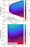 |
Fig. B.1. Top panel Growth rate σr normalised by Ω in the (Pm, Λϕ) plane of the axisymmetric AMRI, for a regime typical of DNS (see Table 1, with |Ro| = 0.05, ΛZ = 0, (N/Ω)2 = 1, m = 1). The three criteria (Eq. 9) correspond to the limits of the unstable parameter domain. The blank region corresponds to the stable parameter domain. Bottom panel Same study but for the stellar radiative regime set of parameters, |Ro| = 0.05, m = 1 and (N/Ω)2 = 10. |
A condition for the local approach to be valid is that the unstable modes must remain small compared to the system size and not larger than the typical domain over which the background parameters vary. This motivates us to derive reliable estimates of the characteristic wave-numbers for both the SMRI and the AMRI. For the SMRI, the mode scale corresponds to the balance between magnetic tension, diffusion, and shear. In contrast, the AMRI is constrained by coupled diffusive frequencies that depend on both the magnetic field strength and the stratification. Since the azimuthal magnetic tension does not involve kZ, the AMRI mode scale is governed by different physical effects than in the SMRI and, apart from secondary corrections, is essentially independent of the shear. We note that for both SMRI and AMRI, the most unstable mode has the lowest radial wavenumber of the values considered, kR = kR, min, and we focus our study on the axial wavenumber kZ. In the case of the SMRI (see Fig. B.2), again two regimes can be distinguished from the ratio of magnetic diffusivity and resistivity. The estimate given below Eq. B.1 agrees well with that proposed by Sano & Miyama (1999) for protoplanetary disks, and with Petitdemange et al. (2008) (magnetostrophic regime) and reproduces the numerical values,
 (B.1)
(B.1)
This estimate remains valid for more diffusive regimes (see Fig. B.2 top panel).
For the AMRI modes, Fig. B.2 (bottom panel) shows the wavenumber kZ across different regimes. The coupled diffusive frequencies constrain the mode size as a function of magnetic field strength and stratification. The following estimate reproduces well the observed variation,
![Mathematical equation: $$ \begin{aligned} k_{Z,\mathrm{AMRI} }R = \dfrac{1}{2} \left[ \dfrac{m^2 \Lambda _\phi \mathrm{Pr}{(\mathrm{N}/ \Omega )^2}}{\mathrm{Ek}} \right]^{1/4}. \end{aligned} $$](/articles/aa/full_html/2026/03/aa58545-25/aa58545-25-eq33.gif) (B.2)
(B.2)
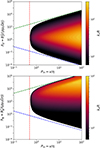 |
Fig. B.2. Top panel: Mode k corresponding to the SMRI modes displayed in Fig. 2 (top panel) Bottom panel: Mode k corresponding to the AMRI modes displayed in Fig. B.1 (top panel). |
Appendix C: Equations governing the magnetic stabilisation of GSF-like instabilities
C.1. Marginal stability equation
When considering a purely axial magnetic field, the marginal stability condition reads
 (C.1)
(C.1)
Some contributions can be directly related to the three SMRI stability criteria introduced in Eq. 9. The SMRI seed term is balanced by:
-
the magnetic stress, which yields the magnetic stress criterion (i),
-
the combined effect of the GSF seed and stabilizing terms, leading to the magnetic diffusion criterion (ii),
-
the magneto-stratification term, associated with the stratification criterion (iii).
In the following, we combine the last two terms under the compact notation (N/Ω)★2 = (N/Ω)2 + 2(κ/η)∂lnΩ/∂lnR. The notation for the last two terms is chosen analogously to the GSF stabilizing contributions. The viscous term is straightforward, while the mixed diffusion term introduces a coupling between magnetic strength (limited by diffusion) and viscosity, thereby connecting both dissipative processes.
Then we can deduce that the GSF modes are constrained by,
 (C.2)
(C.2)
In a compact form these inequalities are expressed as
 (C.3)
(C.3)
with
 (C.4)
(C.4)
C.2. MGSF asymptotic regimes
The minimisation of all stabilizing terms over the mode ranges (kZ, k) is not straightforward. Therefore, to quantify the additional stabilisation induced by an axial magnetic field, we distinguish two regimes. These two underlying minimisation problems arise because depending on the ordering of magnetic, viscous and stratification effects (as specified by Eq. C.2), different terms dominate the stabilisation.
1. First we consider the contributions of viscous and mixed dissipative effects, together with magnetic stress. From the marginal stability equation (Eq. C.1), the boundary of the unstable parameter domain is defined by the mode (kZ, k) minimizing the stabilizing function f(kZ, k) that reads
 (C.5)
(C.5)
Because f increases monotonically with respect to kZ, we use this relation to fix kZ and minimise f with respect to k. Solving the resulting equation ∂kf = 0 for k4 gives the unique positive root, which we denote as kf,
 (C.6)
(C.6)
The corresponding minimum value of the function, f, is then,
 (C.7)
(C.7)
2. In a second regime, we considered viscous diffusion and the interplay between magnetic and stratification effects. The stabilizing function is expressed as
 (C.8)
(C.8)
The two interior stationarity conditions ∂g/∂kZ = 0 and ∂g/∂k = 0 lead to incompatible relations between k and kZ, and therefore no interior extremum exists in the (kZ, k) domain. The minimum must lie on the boundary of the admissible region and we evaluate g at kZ = kZ, min. Using the same method as before, the stabilizing contribution is minimised with respect to k at
 (C.9)
(C.9)
so that the minimum value of g is
![Mathematical equation: $$ \begin{aligned} \begin{aligned} \mathcal{C} _2 = \text{ min}_{(k_Z,k)}g = \dfrac{5}{2}\left(\dfrac{2}{3}\right)^{3/5} \Big [\mathrm{Ek}k_{Z, min}^2 (\Lambda \mathrm{Pr}{(\mathrm{N}/ \Omega )^2}_\star )^{3}\Big ]^{1/5}. \end{aligned} \end{aligned} $$](/articles/aa/full_html/2026/03/aa58545-25/aa58545-25-eq43.gif) (C.10)
(C.10)
Finally, since g(kZ, kg) is strictly decreasing as kZ decreases, the global minimum of g over the allowed domain is indeed reached at the lowest admissible vertical wavenumber kZ = kZ, min, which validates our assumption.
C.3. MGSF stability criteria
In order to obtain a sufficient MGSF stability criterion, we consider the minimisation relation min(kZ, k)(f + g)≥min(kZ, k)f + min(kZ, k)g, combine the minimum values of f and g independently, and get
 (C.11)
To get a more strict criterion, we assume that the instability boundary is controlled by the two asymptotic branches identified above, and we evaluate the marginal stability kf and kg. This time we consider the minimisation relation min(kZ = kZ, min, k ∈ [kf, kg])(f + g)≥min(kZ, k)(f + g). By doing so we obtain the necessary MGSF stability criteria,
 (C.12)
The relevance of the last criteria (Eq. C.12) is illustrated in Fig. 5, where the associated grey dashed line, representing the most restrictive necessary condition, closely follows the numerically determined boundary of the unstable parameter domain. Finally, because of the dependence of C2 ∝ [(ν/κ)(N/Ω)2]3/5, the standard GSF balancing term (ν/κ)(N/Ω)2 ultimately dominates at large stratification numbers. Moreover, since (N/Ω)★2 represents the effective stratification arising from the SMRI balance (Eq. 9,iii), it is negative in the SMRI parameter regime. Therefore, when estimating the minimal shear |Ro, min| required for the onset of the MGSF instability, but not the SMRI, we obtain
![Mathematical equation: $$ \begin{aligned} \vert R_{o,min}\vert \in \Big [1 + \mathrm{Pm}+ \dfrac{8\mathcal{C} _1}{32}, 1 + \mathrm{Pm}+ \dfrac{9\mathcal{C} _1}{32} \Big ]. \end{aligned} $$](/articles/aa/full_html/2026/03/aa58545-25/aa58545-25-eq46.gif) (C.13)
(C.13)
In stellar radiative regions 1 ≫ Pm, so only C1 needs to be retained, and this results applies throughout the entire MGSF parameter domain.
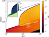 |
Fig. C.1. Mode wavenumber, k, and orientation, kZ/k, for the instabilities found in the regime of Fig. 5. Different instability domains are identified as follows: SMRI⊥ modes share the growth rates of SMRI∥ but are oriented nearly radially. As stratification increases, the SMRI branch is stabilised and MGSF modes dominate. These MGSF modes are clearly distinct from SMRI⊥, exhibiting different growth rates, more horizontal orientation (lower kZ/k), and smaller spatial scales (larger k). |
Appendix D: Method for global linear analysis
D.1. Taylor-Couette framework and model assumptions
In the standard Taylor-Couette framework (see Fig. D.1), the background velocity and temperature fields satisfy the diffusive equilibrium conditions, namely ∇2U0 = 0 for the momentum equation and ∇2T0 = 0 for the thermal field. The basic profiles are ΩTC(R) = A + B/R2 and NTC2 = γgdRT0(R) = C/r, with ζ = Rin/Rout, ξ = Ωin/Ωout so that A = Ωin(ξ − ζ2)/(1 − ζ2), B = ΩinRin2(1 − ξ)/(1 − ζ2), and C = RγgdRT0(R) = γg(Tout − Tin)/(ln1/ζ).
Then, the perturbations U′,B′ are expressed in terms of poloidal and toroidal components,
 (D.1)
(D.1)
and together with the thermal perturbation, T′ (noted j in analogy with Child et al. (2015)), we recover the system of five coupled linear equations. In the notation of Child et al. (2015), the discretised system is expressed as
 (D.2)
(D.2)
where Re = ΩinRin2/ν is the Reynolds number,  the Hartmann number (with B = B0(δeZ + βIRin/R)eϕ)), and we denote J2 = Δj, J5 = −[iRePrm + Δ − (1/R)∂R − ∂R2]j, F5 = Δf and Δ = kZ2 + m2/R2. We expand the spatial structure of the perturbations onto a truncated spectral basis of Nrp Chebyshev polynomials, and we find the eigenmodes using the same numerical method as described in Section A.
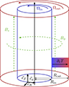 |
Fig. D.1. Sketch of the system under study, showing a shear flow located between two differentially rotating cylinders, subject to a radial thermal gradient and immersed in a magnetic field with axial and azimuthal components. |
For the velocity, we adopt standard no-slip boundary conditions. For the magnetic field, we consider two types: perfectly conducting boundaries, defined by bR = bϕ/R + dRbϕ = 0, and insulating boundaries, defined by ∇ × b|in/out = 0. In the insulating case, unstable modes can be confined in a thin region near the inner cylinder, with components that neither decay nor oscillate coherently. These correspond to wall modes and are not physically relevant, as coherent evolution of all field components is expected in realistic flows. Since our goal is to apply these results to stellar interiors, where no solid boundaries exist, the qualitative stability properties are not expected to depend strongly on the precise boundary choice. We therefore adopt perfectly conducting boundary conditions in this study.
Unless specified, in the dimensionless parameters used (Table 1) to specify the regime studied, we adopt the maximum values of the angular velocity, Brunt–Väisälä frequency and azimuthal magnetic field profiles, and the typical length scale is  , following Rüdiger et al. (2010). For instance, we note ΛZ = BZ2/(ρμ0Ωinη) and
  .
.
D.2. Other examples of mode localisation
In Fig. D.2 (top panel), we consider a steep Taylor-Couette thermal profile, N2 = NR = Rin2(Rin/R)2, together with an ad hoc rotation profile Ω(R) chosen such that the shear Ro = (R/2Ω)dRΩ remains constant. The parameters are Ek = 10−5, Λ = 1.6, Pm = 1, Pr = 0.1. For several shear values, we display the radial velocity perturbations, with the local growth rate estimate along the radius shown in red. Discrepancies in the mode location are interpreted as arising from the nearly flat local growth rate profile, where non-local effects, such as curvature and boundary conditions, influence the position. We also note that the radial mode scale appears correlated with the sharpness of the local growth rate profile. The numerical growth rate is again in good agreement with the maxima reached by the analytical formula (Eq. 11) in the domain. Their ratio lie in [0.98, 1.16], and as suggested by the local approach, the axial wavenumber scaling  is recovered, see Table D.2.
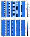 |
Fig. D.2. Top panel: Reconstructed radial velocity perturbations U′R(R, Z) of the most unstable SMRI eigenmode in the following regime, Ek = 10−5, Λ = 1.6, Pm = 1, Pr = 0.1, β = 0 for a radial stratification (N/Ω)2(R) = 1.3/R2 and 5 different rotation profiles Ω(R) = Ωinr−2Ro with a constant shear |Ro| of 0.1, 0.2, 0.25, 0.3 and 0.5. The fastest growth rate computed is given below the shear value considered. The red overlayed curves correspond to the local estimate (Eq. 11). The other perturbations Uϕ′,U′Z, B′R, B′ϕ, B′Z, T′ are located in the same regions. Bottom panel: Same for AMRI eigenmode with m = 2 and in the following regime, Ek = 105, Λϕ = 2.5 × 10⁴, Pm = 2, Pr = 0.001, (N/Ω)2(R) = 100/R2 and 5 different rotation profiles Ω(R) = Ωinr−2|Ro| with a constant shear |Ro| of 0.1, 0.2, 0.25, 0.3 and 0.5. |
Stability properties for the Star A (rb = 0.0146R★, wb = 0.0234R★, Ωin = 3.17 × 10⁻⁶s−1) and the Star F (rb = 0.0092R★, wb = 0.0084R★, Ωin = 1.03 × 10⁻⁵s−1) for different profiles (rd, wd, BZ, 0).
In Fig. D.2 (bottom panel), we perform a similar analysis for the AMRI, for the same kind of N2(R) and Ω(R) profiles, with an azimuthal magnetic field and perturbations with azimuthal wavenumber m = 2 and a different set of flow parameters, Ek = 105, Λϕ = 2.5 × 10⁴, Pm = 2, Pr = 0.001, (N/Ω)2 = 100. We find a good correlation between the mode localisation and the maximum of the local growth rate profile, with comparable values. However, for parameter regimes closer to the stability boundary in the parameter space, the correlation becomes less robust, suggesting that curvature or boundary effects may play a significant role.
D.3. Numerical stability of global MGSF modes
In Fig. 8, the global modes grow more slowly than predicted by the local analytical formula (Eq. 17). We remark that the GSF and MGSF growth rates are sensitive to the radial resolution parameter Nrp (here Nrp = 40). Increasing Nrp slightly raises the ratio between numerical and local values, suggesting that the preferred radial scale of GSF modes is very small and requires high resolution to be properly resolved. This behaviour is consistent with the local analysis of the MGSF (Fig. 4 bottom panel), involving fine spatial scales. At the same time, higher resolution enlarges the parameter range where spurious eigenvalues appear. For the regime displayed in Fig. 8, we made sure to achieve numerical convergence for the entire unstable parameter space.
Axial wavenumber of the most unstable SMRI modes.
Appendix E: Instability properties for different models of subgiants and young RGB stars
In Table D.1, we summarise the instabilities and their properties for models with the different rotation and magnetic-field profiles described in Sect. 4. The large variability in the instability growth times indicates that stellar parameters shape instabilities of widely differing efficiencies, highlighting the need to include these effects in order to obtain realistic estimates of angular momentum transport throughout stellar evolution.
All Tables
Dimensionless parameter set (Prandtl, magnetic Prandtl, Ekman, Elsässer, azimuthal Elsässer, stratification, and shear-rate number), with typical values used in DNS and estimates for stellar radiative regions.
Input parameters and surface properties of the stellar models of stars A and F in the D14 stellar sample, computed with the newest version of Cesam2k20.
Stability properties for the Star A (rb = 0.0146R★, wb = 0.0234R★, Ωin = 3.17 × 10⁻⁶s−1) and the Star F (rb = 0.0092R★, wb = 0.0084R★, Ωin = 1.03 × 10⁻⁵s−1) for different profiles (rd, wd, BZ, 0).
All Figures
|
Fig. 1. Sketch of the system under study. In the inertial frame, the differentially rotating flow is confined between two shells, subjected to a radial thermal gradient and immersed in a magnetic field with both axial and azimuthal components. |
| In the text | |
|
Fig. 2. Top panel: Growth rate, σr, normalised by Ω in the (Pm, ΛZ) plane of the axisymmetric SMRI, for a regime typical of DNS. See details in Table 1, with Ro = −0.05, (N/Ω)2 = 1, Λϕ = 0. The three dashed lines correspond respectively to the three criteria Equation (9). The blank region corresponds to the stable parameter domain. The dotted lines correspond to ΛZ, L, ΛZ, U, from the Eq. (12), when ΛZ, U > ΛZ, L. Bottom panel: Growth rate, σr, normalised by Ω in the (Pm, ΛZ) for a regime of radiative stellar region (see Table 1, with Ro = −0.05, (N/Ω)2 = 10, Λϕ = 0). |
| In the text | |
|
Fig. 3. Growth time, τr/τΩ (=Ω/σr), as a function of Λ for different magnetic-field configurations, parametrised by ΛZ = δ2Λ, Λϕ = β2Λ. We consider regimes representative of stellar radiative zones (Table 1): a weakly stratified, low-shear case (|Ro| = 0.5, (N/Ω)2 = 1) relevant to the MRI, and a strongly stratified, high-shear case (|Ro| = 5, (N/Ω)2 = 5 × 10³) relevant to the GSF and MGSF instability (Sect. 3). The dotted lines show the analytical growth rate estimates (Eqs. (11), (13), and (17)). |
| In the text | |
|
Fig. 4. Top panel: Growth rate σr/Ω in the (|Ro|,(N/Ω)2) of the SMRI, GSF and SH instabilities, for a regime typical of radiative regions (see Table 1, ΛZ = 100, Λϕ = 0). The three dashed lines correspond to instability thresholds, red for SMRI (Eq. (9)), blue for GSF, green for SH. The dotted lines separate the dominant type of instability inside the unstable domain from the mode properties. Bottom Panel: Stability map in the (k, α) plane for a stellar regime with |Ro| = 3 and ΛZ = 100. Solid colored curves show the boundaries of the unstable domains for several values of the stratification parameter (N/Ω)2. The blue region corresponds to the unstable range for (N/Ω)2 = 10, and the star markers indicate, for each (N/Ω)2, the most unstable mode (corresponding to the regimes indicated by the stars in the top panel). The black region denotes modes excluded by our assumptions. The densely dashed horizontal line indicates the upper limit of the GSF-unstable domain set by magnetic stresses. The dashed lines show the modified stability boundaries due to the combined action of magnetic stresses and stratification, shown here for (N/Ω)2 = 5 × 10³ and 5 × 10⁵. The loosely dashed line marks the limit imposed by viscous diffusion. Labels indicate the domains of SMRI‖, SMRI⊥, and MGSF modes. |
| In the text | |
|
Fig. 5. Ratio of the growth rate σr to the analytical formula σestim ≡ max(σSMRI, σMGSF), which combines the predictions for SMRI (Eq. (11)) and MGSF (Eq. (17)). The flow parameters correspond to those of Fig. 4 (top panel), with ΛZ = 105. The white dotted lines delimit the different instability domains (see Appendix C and Fig. C.1 for details). The black dashed line indicate the sufficient MGSF stability criterion (Eq. (15)). The grey dotted line correspond to the combination of the necessary criteria (Eq. (C.12)). See Appendix C.3 for details. |
| In the text | |
|
Fig. 6. Top panel: Ratio σr/σSMRI, R = Rin in the (Pm, ΛZ) plane of the SMRI for regimes with Pr = 10−3, Ek = 10−5, Ro = −0.5, (N/Ω)2 = 102. The estimate σSMRI, R = Rin comes from the local model Eq. (11) evaluated at R = Rin and σr corresponds to the numerical values obtained with the global code. The green, red and blue dashed lines correspond to the criteria introduced in the local approach (Eq. (9)). Bottom panel: Ratio σr/σAMRI, R = Rin in the (Pm, Λϕ) plane of the Azimuthal MRI for the same regime than top panel and considering the fastest mode among the set of azimuthal wavenumbers m ∈ [1, 2, 5, 7, 10] and σAMRI, r = Rin from Eq. (13). The blue and green dashed lines corresponds to the criteria for m = 1 (Eq. (9)). The dashed lines indicate the parameter region in which a given azimuthal mode number, m, yields the maximum growth rate. |
| In the text | |
|
Fig. 7. Reconstructed radial velocity perturbations U′R(R, Z) of the most unstable eigenmode in regimes with ΛZ = 1.6, Ek = 10−5, Pm = 1, Pr = 0.1, at R = Rin and stratification amplitudes (N/Ω)2R = R∈in of 1, 1.3, 1.5, 2, and 2.5. The maximal shear is |Romax| = 0.05. The corresponding growth rate computed is given below the stratification value considered. The red overlayed curves correspond to the analytical formula (Eq. (11)). The vertical black dashed lines give the radius where the mode amplitude peaks and the vertical red dashed lines give the radius where the analytical formula reaches its maximum. |
| In the text | |
|
Fig. 8. Ratio σr/σMGSF, R = Rin in the (ΛZ, Ek) plane for the MGSF, with Pm = 0.1, Pr = 10−2, Ro = −6, (N/Ω)2 = 400, and Λϕ = 0 and the resolution, Nrp = 30. Shear and stratification are constant across the domain, as are the Elsässer and Ekman numbers. The green dashed line marks the MGSF stability criterion (Eq. (15)). |
| In the text | |
|
Fig. 9. Growth rates of unstable regions for different rotation and Brunt-Väisälä (BV) frequency profiles, shown in the background color scale, are displayed for the stars considered. The type of shear-driven instability (e.g. SMRI, MGSF) is indicated in each panel. The BV profile exhibits a narrow peak corresponding to the hydrogen-burning shell. Its position defines the reference radius, rb. The reference width, wb, is defined as the radial distance over which the BV frequency decreases by an order of magnitude from its maximum at rb. Left panels: Star A, top:BZ, 0 = 1 kG, wd = wb, rd = 5rb. Bottom:BZ, 0 = 100 kG, linear rotation profile Ω(r). Right panels: Star F, top:BZ, 0 = 1 G, wd = 3wb, rd = 2rb. Bottom:BZ, 0 = 100 kG, wd = 5wb, rd = 2rb. |
| In the text | |
|
Fig. B.1. Top panel Growth rate σr normalised by Ω in the (Pm, Λϕ) plane of the axisymmetric AMRI, for a regime typical of DNS (see Table 1, with |Ro| = 0.05, ΛZ = 0, (N/Ω)2 = 1, m = 1). The three criteria (Eq. 9) correspond to the limits of the unstable parameter domain. The blank region corresponds to the stable parameter domain. Bottom panel Same study but for the stellar radiative regime set of parameters, |Ro| = 0.05, m = 1 and (N/Ω)2 = 10. |
| In the text | |
|
Fig. B.2. Top panel: Mode k corresponding to the SMRI modes displayed in Fig. 2 (top panel) Bottom panel: Mode k corresponding to the AMRI modes displayed in Fig. B.1 (top panel). |
| In the text | |
|
Fig. C.1. Mode wavenumber, k, and orientation, kZ/k, for the instabilities found in the regime of Fig. 5. Different instability domains are identified as follows: SMRI⊥ modes share the growth rates of SMRI∥ but are oriented nearly radially. As stratification increases, the SMRI branch is stabilised and MGSF modes dominate. These MGSF modes are clearly distinct from SMRI⊥, exhibiting different growth rates, more horizontal orientation (lower kZ/k), and smaller spatial scales (larger k). |
| In the text | |
|
Fig. D.1. Sketch of the system under study, showing a shear flow located between two differentially rotating cylinders, subject to a radial thermal gradient and immersed in a magnetic field with axial and azimuthal components. |
| In the text | |
|
Fig. D.2. Top panel: Reconstructed radial velocity perturbations U′R(R, Z) of the most unstable SMRI eigenmode in the following regime, Ek = 10−5, Λ = 1.6, Pm = 1, Pr = 0.1, β = 0 for a radial stratification (N/Ω)2(R) = 1.3/R2 and 5 different rotation profiles Ω(R) = Ωinr−2Ro with a constant shear |Ro| of 0.1, 0.2, 0.25, 0.3 and 0.5. The fastest growth rate computed is given below the shear value considered. The red overlayed curves correspond to the local estimate (Eq. 11). The other perturbations Uϕ′,U′Z, B′R, B′ϕ, B′Z, T′ are located in the same regions. Bottom panel: Same for AMRI eigenmode with m = 2 and in the following regime, Ek = 105, Λϕ = 2.5 × 10⁴, Pm = 2, Pr = 0.001, (N/Ω)2(R) = 100/R2 and 5 different rotation profiles Ω(R) = Ωinr−2|Ro| with a constant shear |Ro| of 0.1, 0.2, 0.25, 0.3 and 0.5. |
| In the text | |
Current usage metrics show cumulative count of Article Views (full-text article views including HTML views, PDF and ePub downloads, according to the available data) and Abstracts Views on Vision4Press platform.
Data correspond to usage on the plateform after 2015. The current usage metrics is available 48-96 hours after online publication and is updated daily on week days.
Initial download of the metrics may take a while.