© The Authors 2026

1. Introduction

The recent detection of equatorial Rossby waves (e.g. Papaloizou & Pringle 1978; Saio 1982) in the Sun (Löptien et al. 2018) has reinvigorated interest in the study of the gravito-inertial modes of oscillation in solar-type stars (e.g. Jain et al. 2024). In particular, Hindman & Jain (2023) demonstrate that thermal Rossby waves, a class of gravito-inertial waves trapped in the convective envelope (Hindman & Jain 2022; Hanasoge 2026) that are distinct from equatorial Rossby waves and also referred to as convective modes, are able to couple with the prograde g modes trapped in the radiative interior. The observation and characterisation of such a coupling between radiative interior g modes and envelope inertial modes of oscillation would open up new perspectives and allow us to probe the deepest stellar layers. However, in a star rotating as slowly as the Sun, this coupling can only act at very low frequencies, making a detection attempt observationally challenging in the context of asteroseismology because it would require extremely long time series, as well as exceptional instrumental stability at low frequencies. On the contrary, young solar-type stars rotate significantly faster before they enter the main sequence (e.g. Gallet & Bouvier 2015) and spin down under the action of magnetic braking (e.g. Weber & Davis 1967; Skumanich 1972). This would enable the eigenfrequencies of the inertial modes to extend towards larger values, in frequency intervals more easily accessible to space-borne photometry (see e.g. Messina et al. 2024 for a candidate signature in an M dwarf). With respect to other stages of evolution, a relatively small number of studies have been dedicated to the asteroseismology of pre-main-sequence (PMS) stars (see Zwintz & Steindl 2022, for a review). As progenitors of the systems we observe on the main sequence, they are nevertheless of primary importance to our understanding of the history of older targets.

In this Letter we show that in PMS stars, g modes and envelope inertial waves are able to couple in frequency ranges that can reasonably be accessed by photometric instruments such as Kepler/K2 (Borucki et al. 2010; Howell et al. 2014), the Transiting Exoplanet Survey Satellite (TESS; Ricker et al. 2015), and the PLanetary Transits and Oscillations of star mission (PLATO; Rauer et al. 2025). In Sect. 2 we present the stellar models we used for the study, while in Sect. 3 we compute the eigenfunctions of the gravito-inertial modes and show that the radiative-convective coupling induces an inertial dip that can be described asymptotically by a Lorentzian profile depending on the rotation frequency and on the stiffness of the convective-radiative interface. Our conclusions and perspectives are given in Sect. 4.

2. Stellar models

2.1. Structure models

To illustrate the possibility of a coupling between g modes and envelope inertial waves, we considered the case of a K-type and a G-type PMS progenitor at solar metallicity, with masses M_★ = 0.5 M_⊙ and 1 M_⊙, respectively. Their properties are summarised in Table A.1. We used the PMS evolutionary tracks computed by Steindl et al. (2021) with the Module for Experiments in Stellar Astrophysics (MESA; Paxton et al. 2011). These PMS models assume constant accretion until a star reaches its current mass, starting from an initial seed with mass 0.01 M_⊙. The models were then evolved until the start of the hydrogen burning phase at the zero-age main sequence (ZAMS). The evolutionary tracks for the two selected models are represented in Fig. A.1 from the end of the accreting phase to the ZAMS. We considered the structure of the 0.5 M_⊙ model at 21.4 Myr and of the 1 M_⊙ one at 12.4 Myr. We note that we limited ourselves to the case of structure models with a radiative interior and a convective envelope, as the complex mode coupling that would be induced by the combination of a convective core, a radiative interior, and a convective envelope is beyond the scope of this work.

2.2. Rotational evolution

The rotational evolution of the two models was computed a posteriori, considering that the radiative-convective coupling timescale for the transport of angular momentum is short enough to assume solid-body rotation (e.g. Spada et al. 2011). We accounted for wind braking and for a disc-coupling phase at the end of the accretion phase. We considered the cases of a slow, an intermediate, and a fast initial rotation rate, with Ω_★, init = 3.2, 8, and 18 Ω_⊙, respectively. This rotation rate was set to be constant during the disc-coupling phase, which lasts 6 Myr in the slow and intermediate cases, and 2 Myr in the fast case. Then, during the PMS phase, the star spins up due to contraction, although a fraction of its angular momentum is already lost due to stellar magnetised wind. The prescription used to account for the magnetic braking of the stellar surface comes from Matt et al. (2015, 2019). The free parameters of this prescription have been calibrated to reproduce the surface rotation of the Sun (Eggenberger et al. 2019). The Ω_★, init values and the relative disc-locking timescales for the fast and slow rotators have been calibrated to reproduce the spread of surface rotation rates observed for stars in open clusters and stellar associations (Gallet & Bouvier 2015).

The rotational evolution during the span of the evolutionary tracks represented in Fig. A.1 is illustrated in Fig. A.2. For the reference age and structure we considered here, for the 0.5 M_⊙ and 1 M_⊙ models, respectively, the models with a low initial rotation rate have a rotation frequency of Ω_★ = 4.5 and 4.7 Ω_⊙; models with intermediate rotation have Ω_★ = 12.0 and 11.6 Ω_⊙; and models with fast rotation have Ω_★ = 38.4 and 45.4 Ω_⊙. This final set of values corresponds to ratios of Ω_★/Ω_c = 0.11 and Ω_★/Ω_c = 0.22, where Ω_c = (GM_★/R_★³)^1/2 is the critical Keplerian frequency. Although this places the fast case at the limit of the Ω_★/Ω_c ≪ 1 assumption, in the following, we neglect the impact of the centrifugal acceleration in order to model our star using 1D non-deformed profiles and, therefore, to preserve the simplicity of the physical scenario we aim to describe here.

3. Mode coupling

In the following, we use the equatorial model presented in Appendix B.1 (see also Ando 1985; Mathis et al. 2023; Jain et al. 2024). We restricted the problem to the equatorial frame in order to account for the full Coriolis force (Ando 1985; Mathis et al. 2023). This allowed us to grasp qualitatively the physical picture of the impact that the non-traditional component of the Coriolis force has on these waves, which are confined close to the equator (Jain & Hindman 2023). We numerically solved the linearised Euler equations in the Cowling (1941) approximation, assuming spherical symmetry for the equilibrium quantities:

$$\begin{array}{cc}\hfill {\xi }_{r}r& =-(\frac{1}{r}(2+\frac{m\zeta }{\omega })+\frac{1}{{\mathrm{\Gamma }}_1}lnpr){\xi }_r+\frac{1}{\rho c_s^2}(\frac{S_{\stackrel{\sim }{\ell }}^2}{{\omega }^2}-1)p\prime ,\hfill \end{array}$$(1)

$$\begin{array}{cc}\hfill p\prime r& =\rho ({\omega }^2-N^2-2\mathrm{\Omega }\zeta ){\xi }_r+(\frac{1}{{\mathrm{\Gamma }}_1}lnpr+\frac{2\mathrm{\Omega }m}{\omega r})p\prime ,\hfill \end{array}$$(2)

where ω is the wave local angular frequency, r the stellar radius, p the equilibrium pressure, ρ the equilibrium density, c_s the sound speed, N² the Brunt-Väisälä frequency, Γ₁ = (∂lnp/∂lnρ)_ad the adiabatic exponent, Ω the rotation profile, and ζ = 2Ω + r(dΩ/dr) the stellar vorticity. The local frequency, ω, is related to the inertial frequency, ω_in, through the relation ω = ω_in − mΩ. The perturbed quantities for which eigenfunctions are searched for are ξ_r, the radial displacement, and p′, the Eulerian pressure perturbation. Finally, m is the azimuthal number, and $\stackrel{\sim }{\ell }$ is the global horizontal degree; the Lamb frequency, $S_{\stackrel{\sim }{\ell }}$, can therefore be written as $S_{\stackrel{\sim }{\ell }}^2=\stackrel{\sim }{\ell }(\stackrel{\sim }{\ell }+1)c_s^2/r^2$, with a sound speed of $c_s=\sqrt{{\mathrm{\Gamma }}_{1}p/\rho }$. In the case without rotation, Eqs. (1) and (2) simply correspond to the second-order system of stellar oscillations in the Cowling approximation (e.g. Aerts et al. 2010). In the following, we consider dipolar prograde modes with $\stackrel{\sim }{\ell }=m=1$.

As discussed in Appendix B.2, the propagation of the gravito-inertial waves will be constrained by the shape of the buoyant and Coriolis cavities, which are related to the N and 2Ω frequencies, respectively. Roughly, from Eq. (B.38), for dipolar prograde modes, the mode will have an oscillating behaviour when

$$\begin{array}{c}\hfill {\omega }^2<N^2+4{\mathrm{\Omega }}^2(1-\frac{m^2}{\stackrel{\sim }{\ell }(\stackrel{\sim }{\ell }+1)})=N^2+2{\mathrm{\Omega }}^2.\end{array}$$(3)

In Fig. 1 we show the propagation regions of the waves as a function of frequency. We note that in the bulk of the convective envelope, |N²|≪4Ω², where 4Ω² is the squared Coriolis frequency. In the radiative interior, N² ≫ 4Ω² in the slow case but not in the fast case. In addition, below a given radius, we have N² < 4Ω². It is also visible that the convective envelope of the 0.5 M_⊙ model has a larger extension, with its bottom located at r_cz = 0.38 R_★, while r_cz = 0.59 R_★ for the 1 M_⊙ stellar model.

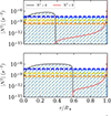Fig. 1. Modulus of the squared Brunt-Väisälä frequency, |N2|, for the 0.5 M⊙ model (top) and the 1 M⊙ model (bottom). Regions where N2 ≥ 0 are in gray, and regions where N2 < 0 are in red. The squared Coriolis frequency, 4Ω2, is indicated by the horizontal dashed line for the slow (orange), the intermediate (yellow), and the fast (blue) cases, while the horizontal dotted lines correspond to 2Ω2. The propagation region of gravito-inertial waves as a function of frequency is highlighted by the hatched areas (orange dots and blue hatches for the slow and fast cases, respectively).

The method we used to numerically compute the eigenfunctions of our stellar models is detailed in Appendix B.4. For each stellar model, we first searched for eigenfunctions that are solutions to the system defined by Eqs. (1) and (2), considering the full extent of the stellar structure. We then restricted the domain to the extent of the convective envelope. The eigenfunctions were computed with the open source mascaret¹ module, which implements a double shooting scheme to identify the eigenvalues of the system (Press et al. 1992). At low frequencies, we limited our search to ω/(2π) = 1 μHz, which corresponds to a period in the co-rotating frame of about 11.57 days. Given that m = 1, in the inertial frame, the eigenfrequencies will be shifted towards larger values. We computed ΔP as the period spacing between the periods in the co-rotating frame, P, of modes with consecutive radial order n. For the three rotation regimes, the ΔP versus P diagram we obtained for the computation considering the full extent of the stellar structure is represented in Fig. 2. For comparison, we also show in Fig. B.2 the inertial period spacing, ΔP_in, versus ω_in diagram (ΔP_in is the directly observable quantity). In the fast and intermediate cases, the ΔP pattern is strongly affected by the coupling with the envelope inertial modes. The periods of the eigenmodes obtained when restricting the computation to the convective envelope are highlighted in Fig. 2. Around the eigenfrequencies of these envelope eigenmodes, the coupling between the g modes trapped in the radiative interior and a gravito-inertial mode from the envelope is clearly visible as sudden drops in the ΔP pattern, referred to as inertial dips (Ouazzani et al. 2020; Saio et al. 2021). Away from the dips, the ΔP pattern also significantly differs between the slow and the fast cases, reflecting the contribution from the Coriolis acceleration to the mode dynamics: in the radiative interior, the Coriolis contribution enforces the effective stratification of the medium, reducing the period spacing between consecutive modes (see Eq. (B.36)). In addition, notwithstanding the strength of the coupling, all modes with P > 1/(2Ω_★) are in the sub-inertial regime and the corresponding waves remain propagative even in the convective envelope. Concerning the slow rotation case, there is no inertial dip at periods shorter than 12 days for the 1 M_⊙ model. Nevertheless, the first inertial dip is visible around P = 11 days for the 0.5 M_⊙ model. It is possible to show that each of these inertial dips can be described asymptotically with a Lorentzian profile (Tokuno & Takata 2022; see Appendix B.3 for the derivation in the case of our equatorial formalism),

$$\begin{array}{c}\hfill \mathrm{\Delta }P=\mathrm{\Delta }{P}_0(1-\frac{\mathrm{\Delta }{P}_0\sigma /\pi }{{(P-P_{\ast }+\sigma /\sqrt{3})}^2+{\sigma }^2+\mathrm{\Delta }{P}_0\sigma /\pi }),\end{array}$$(4)

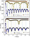Fig. 2. Top: ΔP vs P diagram for the $\stackrel{\sim }{\ell }=m=1$ modes in the 0.5 M⊙ model in the co-rotating frame. The dots correspond to the modes computed considering the full extent of the stellar structure, with the slow case in orange, the intermediate case in yellow, and the fast case in blue. The vertical dashed lines mark the period of the modes computed considering only the convective envelope. The position of the Coriolis frequency, 2Ω, is highlighted for the slow, the intermediate, and the fast cases (vertical thick lines in orange, yellow, and blue, respectively), while the $\sqrt{2}\mathrm{\Omega }$ frequency is indicated with the vertical dotted lines. The location of the modes with the eigenfunctions represented in Fig. 3 is marked with the light blue stellar symbol. Bottom: Same as the top panel but for the 1 M⊙ model.

where ΔP₀ is given by Eq. (B.49), and the parameter σ depends on Ω and on the stiffness of the squared Brunt-Väisälä frequency, dN²/dr, at the convective–radiative interface, as shown by Eqs. (B.51) and (B.75). As illustrated in Fig. B.1, this asymptotic approximation describes the shape of the inertial dips we obtained from the numerical computations fairly well.

We note the existence of a first dip for both structure models in the fast case, which is not connected to the eigenfrequency of the envelope modes. We interpret this by recalling that in the central regions of the star, the shape of the resonant cavity is strongly modified by the Coriolis force with respect to the Ω = 0 case (see Fig. 1). This first dip therefore most likely reflects the sensitivity of the mode to this deformation.

Finally, in Fig. 3 we compare two eigenfunctions of the 0.5 M_⊙ model, noting that the location of the two modes in the ΔP versus P diagram is highlighted in Fig. 2. The first one, with a radial order of n = −46, is strongly coupled with the envelope mode with n = −4, whereas the second one, with n = −40, is weakly coupled. The oscillating character of ξ_r in the convective envelope is clearly visible for both the strongly and weakly coupled modes, with several radial nodes located above r_cz = 0.38 R_★, highlighting the fact that both modes are in the sub-inertial regime. We note that the eigenfunction of the strongly coupled mode closely follows that of the envelope mode in the convective zone.

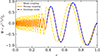Fig. 3. Comparison between the eigenfunctions of the n = −46 (orange) and n = −40 (dotted grey) modes. The eigenfunction of the n = −4 envelope mode is shown in dashed blue.

4. Discussion and conclusion

The coupling between the radiative interior and the convective envelope of the PMS stars appears analogous to the coupling between the convective core and radiative envelope that was seen in γ Dor stars (e.g. Ouazzani et al. 2020; Saio et al. 2021; Tokuno & Takata 2022; Galoy et al. 2024; Barrault et al. 2025b). Different scenarios lead to different observable consequences for the mode amplitudes. On the one hand, convection might transfer energy to the buoyant cavity through penetrative convection (e.g. Alvan et al. 2014; Pinçon et al. 2016; Augustson et al. 2020; Breton et al. 2022) or bulk turbulence (e.g. Belkacem et al. 2009; Lecoanet & Quataert 2013; Mathis et al. 2014; Augustson et al. 2020), as in the traditional g mode picture. On the other hand, convection might be able to transfer its energy to the envelope inertial modes more efficiently (Philidet & Gizon 2023; Fuentes et al. 2026). Therefore, if the excitation in the g mode resonant cavity is the dominating process, the modes should be able to emerge with similar surface amplitudes, even for those with a weak coupling. On the contrary, if the excitation energy is channelled first to the envelope inertial waves before propagating to the radiative interior, the modes with a strong coupling should have a larger surface amplitude. Given that PMS solar-type stars are magnetically active, future works should be aimed at evaluating the impact that an internal magnetic field will have on the shape of the dip (e.g. Barrault et al. 2025a).

In this work we computed the eigenfrequencies for gravito-inertial dipolar prograde modes in 0.5 M_⊙ and 1 M_⊙ PMS stars to illustrate how the coupling between the eigenmodes of the radiative interior and those of the convective envelope of such objects will be affected by rotation. Although the fast rotation regime introduces centrifugal effects that typically deform the stellar cavity, we neglected them to isolate the Coriolis-driven dynamics. The centrifugal distortion would introduce a systematic shift in the eigenfrequencies and slightly modify the cavity geometry, but the fundamental mechanism of the core-envelope coupling and the resulting period-spacing pattern would persist. If the modes are sufficiently excited to induce detectable brightness variations, for fast PMS rotators the coupling will occur in a frequency range that is accessible to space-borne photometry. The imprint it leaves on the mode pattern is expected to provide important information on the mode excitation mechanism. In addition, the analysis carried out in this work demonstrates that these coupled modes should represent powerful seismic probes. Indeed, while the shape of the inertial dips is directly related to the stiffness of the convective–radiative interface, it will also be possible to infer ΔP₀ from the shape of the Lorentzian profile in the ΔP pattern. This will allow us to further probe the characteristics of the deep radiative interior.

Acknowledgments

The authors want to thank the anonymous referee for useful comments. SNB acknowledges support from PLATO ASI-INAF agreement no. 2022-28-HH.0 “PLATO Fase D”. SNB and AFL acknowledge support from the INAF grant MASTODINT. CP thanks the Belgian Federal Science Policy Office (BELSPO) for the financial support in the framework of the PRODEX Program of the European Space Agency (ESA) under contract number 4000141194. S.M acknowledges support from the CNES GOLF-SOHO and PLATO grants at CEA/DAp. LB and SM gratefully acknowledge support from the European Research Council (ERC) under the Horizon Europe programme (LB: Calcifer; Starting Grant agreement N°101165631; SM: 4D-STAR; Synergy Grant agreement N°101071505). While partially funded by the European Union, views and opinions expressed are, however, those of the authors only and do not necessarily reflect those of the European Union or the European Research Council. Neither the European Union nor the granting authority can be held responsible for them. The authors acknowledge G. Buldgen, H. Dhouib, and M.A. Dupret for fruitful discussions.

References

Appendix A: Model properties

The properties of the stellar models we consider in this work, taken from the PMS stellar models with constant accretion computed by Steindl et al. (2021), are summarised in Table A.1, while the evolutionary tracks computed with MESA and the rotational evolution history diagram are shown in Fig. A.1 and Fig. A.2, respectively. The accretion rate considered to reach the initial mass of each PMS model is 5  ×  10⁶ M_⊙yr⁻¹. In addition, Fig. A.1 shows the location of structure models exhibiting a convective core for the Steindl et al. (2021) models ranging between M_★ = 0.2 M_⊙ and M_★ = 1.5 M_⊙. We note that low-mass models have a convective core in the first epochs after the end of the accreting phase, while many models develop a small convective core just before entering the ZAMS. The lowest mass stars become completely convective before entering the ZAMS. This justifies that the configuration we consider in this work (radiative interior surrounded by a convective envelope, with no convective core) is mostly adapted to PMS stars spun up by contraction, before they develop a convective core.

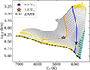Fig. A.1. Evolutionary tracks for the stellar models (0.5 M⊙ in blue and 1 M⊙ in orange) considered in this work, from the end of the accreting phase to the ZAMS. The black thick lines shows the location of the ZAMS. The location on the track of the stellar models we consider in this work is highlighted by the star symbol. The other tracks of the Steindl et al. (2021) PMS grid ranging between M★ = 0.2 M⊙ and M★ = 1.5 M⊙ are shown in grey for comparison, with the structure model saved during the MESA run indicated by grey dots, yellow crosses, and teal plus signs. The crosses signal models which have a convective core while the plus signs correspond to stellar structure that are completely convective.

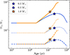Fig. A.2. Rotational evolution computed for the 0.5 (blue) and 1 M⊙ (orange) models. The rotational track with slow initial condition is represented with a dashed line, the track with intermediate initial condition with a dotted line, and the track with fast initial condition with a thick line. The location of the stellar models we consider in this work is highlighted by the star symbol.

Appendix B: Eigenfunction computation

B.1. System derivation

The problem is formulated considering the following set of equations in a differentially rotating star,

$$\begin{array}{cc}\hfill D_t\mathit{V}& =-\frac{1}{\widehat{\rho }}\mathrm{\nabla }\widehat{p}-\mathrm{\nabla }\widehat{\mathrm{\Phi }},\hfill \end{array}$$(B.1)

$$\begin{array}{cc}\hfill \widehat{\rho }t& +\mathrm{\nabla }·(\widehat{\rho }\mathit{V})=0,\hfill \end{array}$$(B.2)

$$\begin{array}{cc}\hfill \frac{1}{{\mathrm{\Gamma }}_1}{D}_{t}ln\widehat{p}& -D_{t}ln\widehat{\rho }=0,\hfill \end{array}$$(B.3)

$$\begin{array}{cc}\hfill {\mathrm{\nabla }}^2\widehat{\mathrm{\Phi }}& =4\pi G\widehat{\rho },\hfill \end{array}$$(B.4)

where the equation are: (in order) the inviscid Euler equation of motion in an inertial reference frame, the equation of continuity, the energy equation in the adiabatic limit, and the Poisson’s equation. G is the gravitational constant and the Lagrangian derivative D_t corresponds to ∂/∂t + V ⋅ ∇. The scalar fields $\widehat{p}$ (pressure), $\widehat{\rho }$ (density), and $\widehat{\mathrm{\Phi }}$ (gravitational potential), are written in all generality and may depend on the time t as well as any spatial coordinate. In spherical coordinates (r, θ, φ), associated with the unit vector basis $({\widehat{\mathit{e}}}_r,{\widehat{\mathit{e}}}_{\theta },{\widehat{\mathit{e}}}_{\phi })$, the velocity field V is

$$\begin{array}{c}\hfill \mathit{V}(r,\theta ,\phi ,t)=rsin\theta \mathrm{\Omega }(r,\theta ){\widehat{\mathit{e}}}_{\mathit{\phi }}+\mathit{u}(r,\theta ,\phi ,t),\end{array}$$(B.5)

where u is the velocity field associated with the wave perturbation, related to the Lagrangian displacement, ξ through (Unno et al. 1989)

$$\begin{array}{c}\hfill \mathit{u}=(t+\mathrm{\Omega }\phi )\mathit{\xi }-rsin\theta (\mathit{\xi }·\mathrm{\nabla }\mathrm{\Omega }){\widehat{\mathit{e}}}_{\phi },\end{array}$$(B.6)

The linearised equations of motion, accounting for the Coriolis force are then, in the Cowling approximation (Unno et al. 1989; Mathis 2009), having expanded the scalar fields $\widehat{X}$ as the sum of an equilibrium quantity X and a perturbation $\stackrel{\sim }{X}\prime$, and assuming that all the equilibrium quantities and the rotation profile Ω depend only on r:

$$\begin{array}{cc}\hfill (t+\mathrm{\Omega }\phi )u_r-2\mathrm{\Omega }sin\theta u_{\phi }& =-\frac{1}{\rho }{\stackrel{\sim }{p}}^{\prime }r-\frac{{\stackrel{\sim }{\rho }}^{\prime }g}{\rho },\hfill \end{array}$$(B.7)

$$\begin{array}{cc}\hfill (t+\mathrm{\Omega }\phi )u_{\theta }-2\mathrm{\Omega }cos\theta u_{\phi }& =-\frac{1}{\rho r}{\stackrel{\sim }{p}}^{\prime }\theta ,\hfill \end{array}$$(B.8)

$$\begin{array}{cc}\hfill (t+\mathrm{\Omega }\phi )u_{\phi }+\zeta u_{r}sin\theta +2\mathrm{\Omega }cos\theta u_{\theta }& =-\frac{1}{\rho rsin\theta }{\stackrel{\sim }{p}}^{\prime }\phi ,\hfill \end{array}$$(B.9)

where g = dΦ/dr. The linearised continuity and energy equations are

$$\begin{array}{c}\hfill \begin{array}{cc}\hfill (t+\mathrm{\Omega }\phi ){\rho }^{\prime }+u_r\rho r& +\rho (\frac{1}{r^2}{r}^2{u}_{r}r\hfill \\ \hfill & +\frac{1}{rsin\theta }sin\theta u_{\theta }\theta +\frac{1}{rsin\theta }{u}_{\phi }\phi )=0,\hfill \end{array}\end{array}$$(B.10)

$$\begin{array}{cc}\hfill (t+\mathrm{\Omega }\phi )(\frac{{\stackrel{\sim }{p}}^{\prime }}{{\mathrm{\Gamma }}_{1}p}-\frac{{\stackrel{\sim }{\rho }}^{\prime }}{\rho })& +u_r(\frac{1}{{\mathrm{\Gamma }}_1}lnpr-ln\rho r)=0.\hfill \end{array}$$(B.11)

Expanding the perturbed quantities $\stackrel{\sim }{X}\prime$ and the component of the displacement and velocity fields in Fourier series such that

$$\begin{array}{c}\hfill {\stackrel{\sim }{X}}^{\prime }(r,\theta ,\phi ,t)={\displaystyle \sum _{k,m}}{X}^{\prime }(r)exp[i({\omega }_{\mathrm{in}}t+k\theta -m\phi )],\end{array}$$(B.12)

where k is the latitudinal wave number, and ω_in is the inertial frequency, connected to the local frequency, ω, through

$$\begin{array}{c}\hfill \omega (r)={\omega }_{\mathrm{in}}-m\mathrm{\Omega }(r).\end{array}$$(B.13)

In this convention, m > 0 corresponds to prograde modes and m < 0 to retrograde modes. Restricting the problem to the vicinity of the equatorial plane (Ando 1985; Mathis et al. 2023), that is considering θ ≈ π/2, allows writing

$$\begin{array}{cc}\hfill -{\omega }^2{\xi }_r-2\mathrm{\Omega }{u}_{\phi }& =-\frac{1}{\rho }{p}^{\prime }r-\frac{{\rho }^{\prime }g}{\rho },\hfill \end{array}$$(B.14)

$$\begin{array}{cc}\hfill -{\omega }^2{\xi }_{\theta }& =-\frac{\mathit{ik}}{\rho r}{p}^{\prime },\hfill \end{array}$$(B.15)

$$\begin{array}{cc}\hfill i\omega u_{\phi }+i\omega \zeta {\xi }_r& =\frac{\mathit{im}}{\rho r}{p}^{\prime },\hfill \end{array}$$(B.16)

$$\begin{array}{cc}\hfill i\omega {\rho }^{\prime }+i\omega \rho r{\xi }_r& +\rho (i\omega [\frac{2}{r}{\xi }_r+{\xi }_{r}r]-\frac{k\omega }{r}{\xi }_{\theta }-\frac{\mathit{im}}{r}{u}_{\phi })=0,\hfill \end{array}$$(B.17)

$$\begin{array}{cc}\hfill \frac{p^{\prime }}{{\mathrm{\Gamma }}_{1}p}& -\frac{{\rho }^{\prime }}{\rho }+\frac{N^2}{g}{\xi }_r=0,\hfill \end{array}$$(B.18)

where the Brunt-Väisälä frequency, N, is defined as

$$\begin{array}{c}\hfill N^2=g[\frac{1}{{\mathrm{\Gamma }}_1}lnpr-ln\rho r].\end{array}$$(B.19)

This equatorial approximation is well suited to characterise the behaviour of gravito-inertial waves that are confined close to the equator (e.g. Townsend 2003; Bekki et al. 2022; Jain & Hindman 2023) without neglecting the non-traditional component of the Coriolis acceleration. Equations B.15 and B.16 can be used to eliminate ξ_θ and u_φ in Eqs. B.14 and B.17 to yield

$$\begin{array}{cc}\hfill (-{\omega }^2+2\mathrm{\Omega }\zeta ){\xi }_r-\frac{2\mathrm{\Omega }m}{\rho r\omega }{p}^{\prime }& =-\frac{1}{\rho }{p}^{\prime }r-\frac{{\rho }^{\prime }g}{\rho },\hfill \end{array}$$(B.20)

$$\begin{array}{c}\hfill \begin{array}{cc}\hfill i\omega {\rho }^{\prime }+i\omega \rho r{\xi }_r& +\rho (i\omega [\frac{2}{r}{\xi }_r+{\xi }_{r}r]\hfill \\ \hfill & -\frac{i{k}^2}{\rho r^2\omega }{p}^{\prime }+\frac{im\zeta }{r}{\xi }_r-\frac{i{m}^2}{\rho r^2\omega }{p}^{\prime })=0,\hfill \end{array}\end{array}$$(B.21)

which can be rewritten

$$\begin{array}{cc}\hfill p^{\prime }r& =\rho ({\omega }^2-2\mathrm{\Omega }\zeta ){\xi }_r+\frac{2\mathrm{\Omega }m}{\omega r}{p}^{\prime }-{\rho }^{\prime }g,\hfill \end{array}$$(B.22)

$$\begin{array}{cc}\hfill {\xi }_{r}r& =(-ln\rho r-\frac{2}{r}-\frac{m\zeta }{\omega r}){\xi }_r+\frac{k^2+m^2}{\rho r^2{\omega }^2}{p}^{\prime }-\frac{{\rho }^{\prime }}{\rho }\hfill \end{array}$$(B.23)

and finally, using Eq. B.18 to express ρ′ in terms of ξ_r and p′, and g = −1/ρ × (dp/dr):

$$\begin{array}{cc}\hfill p^{\prime }r& =\rho [{\omega }^2-N^2-2\mathrm{\Omega }\zeta ]{\xi }_r+[\frac{1}{{\mathrm{\Gamma }}_1}lnpr+\frac{2\mathrm{\Omega }m}{\omega r}]p^{\prime },\hfill \end{array}$$(B.24)

$$\begin{array}{cc}\hfill {\xi }_{r}r& =-\left[\frac{1}{r}\right(2+\frac{m\zeta }{\omega })+\frac{1}{{\mathrm{\Gamma }}_1}lnpr]{\xi }_r\hfill \\ \hfill & +\frac{1}{\rho c_s^2}[\frac{1}{{\omega }^2}\frac{(k^2+m^2)c_s^2}{r^2}-1]p^{\prime },\hfill \end{array}$$(B.25)

where, by making the identification $\stackrel{\sim }{\ell }(\stackrel{\sim }{\ell }+1)=k^2+m^2$ we obtain the system defined by Eqs. 1 and 2. In the case without rotation, the global horizontal number $\stackrel{\sim }{\ell }$ can be identified to the spherical degree ℓ.

It should be noted that the behaviour of equatorial Rossby waves (also known as planetary waves) is not captured by such a model, because it does not include the topological β-effect (that is, the variation with latitude of the strength and direction of the Coriolis force) that is the direct cause for the propagation of the related perturbations. Nevertheless, it fully accounts for sphericity in the radial direction and the compressional β-effect responsible for the propagation of thermal Rossby waves. It is analogous to the millstone model presented by Jain et al. (2024) and the eigenmodes it allows computing in convective envelopes are among the mixed inertial modes they identified.

B.2. Propagation conditions

We can combine Eqs. 1 and 2 to obtain an equation of the form

$$\begin{array}{c}\hfill [2]{\xi }_{r}r+A(r){\xi }_{r}r+B(r){\xi }_r=0,\end{array}$$(B.26)

where, under the assumption of solid body rotation,

$$\begin{array}{cc}\hfill A(r)& =rln\left|\rho r^2{c}_s^2{(\frac{S_{\ell }^2}{{\omega }^2}-1)}^{-1}\right|\hfill \end{array}$$(B.27)

$$\begin{array}{cc}\hfill B(r)& =\frac{1}{c_s^2}(\frac{S_{\stackrel{\sim }{\ell }}^2}{{\omega }^2}-1)(N^2+4{\mathrm{\Omega }}^2-{\omega }^2)-\frac{4{\mathrm{\Omega }}^2{m}^2}{{\omega }^2{r}^2}\hfill \\ \hfill & -\frac{2\mathrm{\Omega }m}{\omega }[\frac{3}{r^2}+\frac{1}{r}\{rln\left|\frac{1}{\rho c_s^2}(\frac{S_{\stackrel{\sim }{\ell }}^2}{{\omega }^2}-1)\right|+\frac{2}{{\mathrm{\Gamma }}_1}lnpr\}]\hfill \\ \hfill & +r\left(\frac{1}{{\mathrm{\Gamma }}_1}lnpr\right)-\frac{2}{r^2}-[\frac{2}{r}+\frac{1}{{\mathrm{\Gamma }}_1}lnpr]rln\left|\frac{1}{\rho c_s^2}(\frac{S_{\stackrel{\sim }{\ell }}^2}{{\omega }^2}-1)\right|\hfill \\ \hfill & -\frac{2}{r}\frac{1}{{\mathrm{\Gamma }}_1}lnpr-\frac{1}{{\mathrm{\Gamma }}_1^2}{\left(lnpr\right)}^2.\hfill \end{array}$$(B.28)

We can then use the following change of variable,

$$\begin{array}{c}\hfill {\xi }_r=C(r)\mathrm{\Psi }(r),\end{array}$$(B.29)

with

$$\begin{array}{c}\hfill C(r)=exp(-\frac{1}{2}{\displaystyle \int }A(r)\mathrm{d}r),\end{array}$$(B.30)

to write

$$\begin{array}{c}\hfill [2]\mathrm{\Psi }r+{\widehat{k}}_r^2\mathrm{\Psi }=0,\end{array}$$(B.31)

with the radial wave vector, ${\widehat{k}}_r^2$, given by

$$\begin{array}{c}\hfill {\widehat{k}}_r^2=B(r)+A(r)lnCr+\frac{1}{C}[2]Cr.\end{array}$$(B.32)

The wave function Ψ thus has an oscillating behaviour only in regions where ${\widehat{k}}_r^2>0$ and is evanescent otherwise. In the low-frequency ${\omega }^2\ll S_{\stackrel{\sim }{\ell }}^2$ limit we have

$$\begin{array}{cc}\hfill \frac{1}{\rho c_s^2}(\frac{S_{\stackrel{\sim }{\ell }}^2}{{\omega }^2}-1)& =\frac{\stackrel{\sim }{\ell }(\stackrel{\sim }{\ell }+1)}{r^2{\omega }^2},\hfill \end{array}$$(B.33)

$$\begin{array}{cc}\hfill C(r)& ={\rho }^{-1/2}{r}^{-2}.\hfill \end{array}$$(B.34)

So, similarly to Press (1981), we have Ψ = ρ^1/2r²ξ_r, and if we neglect the derivative of equilibrium quantities, we get

$$\begin{array}{c}\hfill \begin{array}{c}\hfill {\widehat{k}}_r^2\approx k_r^2\equiv \frac{\stackrel{\sim }{\ell }(\stackrel{\sim }{\ell }+1)}{r^2{\omega }^2}[N_{\mathrm{eff}}^2-{\omega }^2],\end{array}\end{array}$$(B.35)

where we defined

$$\begin{array}{c}\hfill N_{\mathrm{eff}}^2\equiv N^2+4{\mathrm{\Omega }}^2{r}_{\stackrel{\sim }{\ell },m}^2,\end{array}$$(B.36)

with

$$\begin{array}{c}\hfill r_{\stackrel{\sim }{\ell },m}={(1-\frac{m^2}{\stackrel{\sim }{\ell }(\stackrel{\sim }{\ell }+1)})}^{1/2}.\end{array}$$(B.37)

In the limit N² ≫ 4Ω², valid e.g. for the radiative interior, this yields the gravity wave propagation condition while the 4Ω² ≫ N² case corresponds to the pure inertial wave limit. This would occur for example in a convectively neutral medium where N² = 0. In a realistic stellar convective envelope, the super-adiabaticity of the fluid has to be accounted for, and the wave can propagate only if

$$\begin{array}{c}\hfill {\omega }^2<N^2+4{\mathrm{\Omega }}^2{r}_{\stackrel{\sim }{\ell },m}^2,\end{array}$$(B.38)

where it should be kept in mind that N² < 0 in this specific case. Close to the surface, where the derivative of equilibrium quantities are not small with respect to the other terms in Eq. B.32, the propagation condition can be extended to something of the form (Hindman & Jain 2023; Jain & Hindman 2023)

$$\begin{array}{c}\hfill k_r^2+\frac{2\mathrm{\Omega }}{\omega \mathcal{H}}{k}_{\phi }-h(r)>0,\end{array}$$(B.39)

where we follow Jain & Hindman (2023) to define

$$\begin{array}{c}\hfill \frac{1}{\mathcal{H}}=\frac{1}{H_{\rho }}-\frac{2N^2}{g},\end{array}$$(B.40)

where we introduced the density scale height H_ρ = −dr/dlnρ, and k_φ = m/r is the azimuthal wave number, while the h term depends on the derivative of the equilibrium quantities. Under the Lantz-Braginsky-Roberts (Lantz 1992; Braginsky & Roberts 1995) anelastic approximation, it can be shown that h reduces to the acoustic cutoff wavenumber, k_c²,

$$\begin{array}{c}\hfill h\approx k_c^2\equiv \frac{1}{4H_{\rho }}(1-2H_{\rho }r).\end{array}$$(B.41)

B.3. Inertial dips

In this section we adapt the procedure outlined by Tokuno & Takata (2022, hereafter TT22) to derive an analytic approximation for the profile of the inertial dips observed in Fig. 2.

B.3.1. Formulation in the radiative interior

We start by noting that, given the form of k_r, for modes with ${\omega }^2<4{\mathrm{\Omega }}^2{r}_{\stackrel{\sim }{\ell },m}^2$, k_r does not strictly cancel out in the vicinity of the convective-radiative interface and close to the stellar centre. Nevertheless, in the vicinity of these two regions, as long as the Ω value is not too large with respect to ω, we have ω ∼ N_eff and k_r small enough in order to apply the asymptotic treatment that will allow us to obtain an analytic expression for Ψ. We consider that these pseudo-turning points are located at r_a and r_b, located close to the stellar centre and to the convective-radiative interface, respectively. Assuming that we have have the following differential equation for Ψ,

$$\begin{array}{c}\hfill [2]\mathrm{\Psi }r+k_r^2\mathrm{\Psi }\approx 0,\end{array}$$(B.42)

and that it is valid in the vicinity of both r_a and r_b², we therefore have (Unno et al. 1989)

$$\begin{array}{c}\hfill {\mathrm{\Psi }}_1(r)\approx \frac{1}{|k_r{|}^{1/2}}{{\displaystyle \left(\frac{3}{2}\left|{\int }_{r_a}^r|k_r|\mathrm{d}r\right|\right)}}^{1/6}\\ \hfill \times [a\mathrm{Ai}(z_1)+b\mathrm{Bi}(z_1)],\end{array}$$(B.43)

for r ≪ r_b and

$$\begin{array}{c}\hfill {\mathrm{\Psi }}_2(r)\approx \frac{1}{|k_r{|}^{1/2}}{{\displaystyle \left(\frac{3}{2}\left|{\int }_r^{r_b}|k_r|\mathrm{d}r\right|\right)}}^{1/6}\\ \hfill \times [c\mathrm{Ai}(z_2)+d\mathrm{Bi}(z_2)],\end{array}$$(B.44)

for r_a ≪ r. Here a, b, c, and d are constants to determine from the boundary conditions. Ai and Bi are the Airy functions of first and second kind while z₁ and z₂ are given by

$$\begin{array}{cc}\hfill z_1& \equiv \mathrm{sgn}(k_r^2){{\displaystyle \left(\frac{3}{2}\left|{\int }_{r_a}^r|k_r|\mathrm{d}r\right|\right)}}^{2/3},\hfill \end{array}$$(B.45)

$$\begin{array}{cc}\hfill z_2& \equiv \mathrm{sgn}(k_r^2){{\displaystyle \left(\frac{3}{2}\left|{\int }_r^{r_b}|k_r|\mathrm{d}r\right|\right)}}^{2/3}.\hfill \end{array}$$(B.46)

First, we have b = 0 to ensure that the functions decay exponentially below r_a, close to the centre of the star. Then, by matching Ψ₁ to Ψ₂ at r_a ≪ r ≪ r_b, it comes that

$$\begin{array}{cc}\hfill c& =acos{\displaystyle ({\int }_{r_a}^{r_b}{k}_r\mathrm{d}r-\frac{\pi }{2})}=asin\left(\frac{{\pi }^{2}s}{\mathrm{\Omega }\mathrm{\Delta }{P}_0}\right)\hfill \end{array}$$(B.47)

$$\begin{array}{cc}\hfill d& =-asin{\displaystyle ({\int }_{r_a}^{r_b}{k}_r\mathrm{d}r-\frac{\pi }{2})}=acos\left(\frac{{\pi }^{2}s}{\mathrm{\Omega }\mathrm{\Delta }{P}_0}\right),\hfill \end{array}$$(B.48)

where, introducing for convenience the spin parameter s = 2Ω/ω, we have defined (Tassoul 1980)

$$\begin{array}{c}\hfill \mathrm{\Delta }{P}_0\equiv \frac{2{\pi }^2}{\sqrt{\stackrel{\sim }{\ell }(\stackrel{\sim }{\ell }+1)}}{{\displaystyle \left({\int }_{r_a}^{r_b}\frac{N_{\mathrm{eff}}^2}{r}\mathrm{d}r\right)}}^{-1},\end{array}$$(B.49)

and we have computed the ∫k_r term assuming that ω ≪ N. Next, we need to express Ψ and dΨ/dr at r_b. A Taylor expansion around r_b yields

$$\begin{array}{c}\hfill k_r^2\approx {[-\frac{\stackrel{\sim }{\ell }(\stackrel{\sim }{\ell }+1)}{r^2{\omega }^2}{N}^{2}r]}_{r=r_b}(r_b-r)=\frac{\stackrel{\sim }{\ell }(\stackrel{\sim }{\ell }+1)s^2}{{\epsilon }^3{r}_b^3}(r_b-r),\end{array}$$(B.50)

where, under solid-body rotation, dN_eff²/dr = dN²/dr, and we followed TT22 to define

$$\begin{array}{c}\hfill \epsilon \equiv {(-\frac{r_b}{4{\mathrm{\Omega }}^2}{N}^{2}r{|}_{r=r_b})}^{-1/3}.\end{array}$$(B.51)

We note that for r close to r_b with r < r_b, dN²/dr < 0. We have

$$\begin{array}{cc}& \underset{r\to r_b}{lim}\frac{1}{|k_r{|}^{1/2}}{\left(\frac{3}{2}\left|{\int }_{r_a}^r|k_r|\mathrm{d}r\right|\right)}^{1/6}=\frac{{\epsilon }^{1/2}{r}_b^{1/2}}{s^{1/3}{[\stackrel{\sim }{\ell }(\stackrel{\sim }{\ell }+1)]}^{1/6}},\hfill \end{array}$$(B.52)

$$\begin{array}{cc}& \underset{r\to r_b}{lim}r\left[\frac{1}{|k_r{|}^{1/2}}{\left(\frac{3}{2}\left|{\int }_{r_a}^r|k_r|\mathrm{d}r\right|\right)}^{1/6}\right]=0,\hfill \end{array}$$(B.53)

$$\begin{array}{cc}& \underset{r\to r_b}{lim}{z}_{2}r=\frac{s^{2/3}{[\stackrel{\sim }{\ell }(\stackrel{\sim }{\ell }+1)]}^{1/3}}{\epsilon r_b},\hfill \end{array}$$(B.54)

so

$$\begin{array}{c}\hfill \begin{array}{c}\hfill \mathrm{\Psi }(r_b)=\frac{2}{3^{2/3}\mathrm{\Gamma }(2/3)}\frac{a{r}_b^{1/2}{\epsilon }^{1/2}}{s^{1/3}{[\stackrel{\sim }{\ell }(\stackrel{\sim }{\ell }+1)]}^{1/6}}cos(\frac{{\pi }^{2}s}{\mathrm{\Omega }\mathrm{\Delta }{P}_0}-\frac{\pi }{6}),\end{array}\end{array}$$(B.55)

and

$$\begin{array}{c}\hfill \mathrm{\Psi }r{|}_{r=r_b}=\frac{2}{3^{1/3}\mathrm{\Gamma }(1/3)}\frac{a{s}^{1/3}{[\stackrel{\sim }{\ell }(\stackrel{\sim }{\ell }+1)]}^{1/6}}{r_b^{1/2}{\epsilon }^{1/2}}cos(\frac{{\pi }^{2}s}{\mathrm{\Omega }\mathrm{\Delta }{P}_0}-\frac{5\pi }{6}),\end{array}$$(B.56)

where Γ denotes the Gamma function. In what follows, we assume that this approximation for Ψ is valid at r_b = r_CZ.

B.3.2. Formulation in the convective envelope

To find an expression for the wave behaviour in the convective envelope, we look for a solution in the low-frequency limit, ${\omega }^2\ll S_{\stackrel{\sim }{\ell }}^2$, assuming that the wave is trapped between two rigid boundaries at the convective-radiative interface and at the surface, so that

$$\begin{array}{c}\hfill {\xi }_r(r_{\mathrm{CZ}})={\xi }_r(R_{★})=0\Rightarrow \mathrm{\Psi }(r_{\mathrm{CZ}})=\mathrm{\Psi }(R_{★})=0.\end{array}$$(B.57)

We also simplify the problem by assuming N² = 0 everywhere in the convective envelope. This leads to

$$\begin{array}{c}\hfill k_r^2=\frac{\stackrel{\sim }{\ell }(\stackrel{\sim }{\ell }+1)}{r^2{\omega }^2}[4{\mathrm{\Omega }}^2{r}_{\widehat{\ell },m}^2-{\omega }^2],\end{array}$$(B.58)

where k_r² > 0 everywhere when $\omega <2\mathrm{\Omega }{r}_{\stackrel{\sim }{\ell },m}$. We can therefore write Ψ as

$$\begin{array}{c}\hfill \mathrm{\Psi }(r)=A{k}_r^{-1/2}cos({\int }_r^{R_{★}}{k}_r\mathrm{d}r+\varphi ),\end{array}$$(B.59)

where A is an arbitrary constant. The condition Ψ(R_★) = 0 yields ϕ = π/2 and Ψ(r_CZ) = 0 then provides the quantification condition as

$$\begin{array}{c}\hfill sin{\displaystyle \left({\int }_{r_{\mathrm{CZ}}}^{R_{★}}{k}_r\mathrm{d}r\right)}=0\Rightarrow {\displaystyle {\int }_{r_{\mathrm{CZ}}}^{R_{★}}}{k}_r\mathrm{d}r=n_{\ast }\pi ,\end{array}$$(B.60)

where n_* is the radial order of the envelope inertial mode. Given the N² = 0 assumption, we have an analytical solution for ∫k_r:

$$\begin{array}{c}\hfill {\displaystyle {\int }_r^{R_{★}}}{k}_r\mathrm{d}r=\frac{\sqrt{\stackrel{\sim }{\ell }(\stackrel{\sim }{\ell }+1)}}{\omega }{[4{\mathrm{\Omega }}^2{r}_{\widehat{\ell },m}^2-{\omega }^2]}^{1/2}ln\left(\frac{R_{★}}{r}\right),\end{array}$$(B.61)

so that

$$\begin{array}{c}\hfill \begin{array}{cc}\hfill \mathrm{\Psi }(r)=-& A\frac{r^{1/2}}{{[\stackrel{\sim }{\ell }(\stackrel{\sim }{\ell }+1)]}^{1/4}{s}^{1/2}}{[r_{\widehat{\ell },m}^2-\frac{1}{s^2}]}^{-1/4}\hfill \\ \hfill & \times sin(\sqrt{\stackrel{\sim }{\ell }(\stackrel{\sim }{\ell }+1)}s{[r_{\widehat{\ell },m}^2-\frac{1}{s^2}]}^{1/2}ln\left(\frac{R_{★}}{r}\right)).\hfill \end{array}\end{array}$$(B.62)

The latter is null at r_CZ for the pure inertial wave trapped in the convective envelope but not when we will be looking for a continuous solution at the convective-radiative interface. We also have

$$\begin{array}{c}\hfill \begin{array}{c}\hfill \mathrm{\Psi }r{|}_{r=r_{\mathrm{CZ}}}=A{r}_{\mathrm{CZ}}^{-1/2}{[\stackrel{\sim }{\ell }(\stackrel{\sim }{\ell }+1)]}^{1/4}{s}^{1/2}{[r_{\widehat{\ell },m}^2-\frac{1}{s^2}]}^{1/4}\\ \hfill \times cos(\sqrt{\stackrel{\sim }{\ell }(\stackrel{\sim }{\ell }+1)}s{[r_{\widehat{\ell },m}^2-\frac{1}{s^2}]}^{1/2}ln\left(\frac{R_{★}}{r_{\mathrm{CZ}}}\right)).\end{array}\end{array}$$(B.63)

B.3.3. Continuity condition

The Lagrangian pressure perturbation δp and the displacement ξ_r must be continuous at r_CZ. Given that the equilibrium quantity ρ and p are continuous, it is enough to ensure that Ψ and dΨ/dr are too, such that

$$\begin{array}{c}\hfill \mathrm{\Psi }(r_{\mathrm{CZ},-})=\mathrm{\Psi }(r_{\mathrm{CZ},+}),\end{array}$$(B.64)

$$\begin{array}{c}\hfill \mathrm{\Psi }r{|}_{r=r_{\mathrm{CZ},-}}=\mathrm{\Psi }r{|}_{r=r_{\mathrm{CZ},+}}.\end{array}$$(B.65)

Substituting the terms by their analytical expression and dividing Eq. B.64 by Eq. B.65, we get

$$\begin{array}{c}\hfill \begin{array}{cc}\hfill \epsilon & {[tan(\frac{{\pi }^{2}s}{\mathrm{\Omega }\mathrm{\Delta }{P}_0}-\frac{\pi }{6})-\frac{1}{\sqrt{3}}]}^{-1}=\hfill \\ \hfill & \left(\frac{3^{1/3}\mathrm{\Gamma }(2/3)}{\mathrm{\Gamma }(1/3)}\right)\frac{1}{{[\stackrel{\sim }{\ell }(\stackrel{\sim }{\ell }+1)]}^{1/6}{s}^{1/3}}{[r_{\widehat{\ell },m}^2-\frac{1}{s^2}]}^{-1/2}\hfill \\ \hfill & \times tan(\sqrt{\stackrel{\sim }{\ell }(\stackrel{\sim }{\ell }+1)}s{[r_{\widehat{\ell },m}^2-\frac{1}{s^2}]}^{1/2}ln\left(\frac{R_{★}}{r_{\mathrm{CZ}}}\right)).\hfill \end{array}\end{array}$$(B.66)

It is then possible to expand the right-hand term in the vicinity of the point where it vanishes, located at s_*, which is defined as the spin parameter of the isolated envelope inertial mode. We obtain

$$\begin{array}{c}\hfill tan(\frac{{\pi }^{2}s}{\mathrm{\Omega }\mathrm{\Delta }{P}_0}-\frac{\pi }{6})=\frac{\epsilon }{(s-s_{\ast })V}+\frac{1}{\sqrt{3}},\end{array}$$(B.67)

where the term V is given by

$$\begin{array}{c}\hfill \begin{array}{cc}\hfill V=& \left(\frac{3^{1/3}\mathrm{\Gamma }(2/3)}{\mathrm{\Gamma }(1/3)}\right)ln\left(\frac{R_{★}}{r_{\mathrm{CZ}}}\right)\hfill \\ \hfill & \times \frac{{[\stackrel{\sim }{\ell }(\stackrel{\sim }{\ell }+1)]}^{5/6}}{s_{\ast }^{1/3}}[1+\frac{1}{s_{\ast }^2}{(r_{\widehat{\ell },m}^2-\frac{1}{s_{\ast }^2})}^{-1/4}].\hfill \end{array}\end{array}$$(B.68)

We now consider two neighbouring modes with spin parameters s₁ and s₂, and periods P₁ and P₂ such that s₂ > s₁, P₂ > P₁, where we recall that s = ΩP/π. We also define $\overline{s}=(s_1+s_2)/2$. We have (TT22)

$$\begin{array}{c}\hfill \frac{{\pi }^2(s_2-s_1)}{\mathrm{\Omega }\mathrm{\Delta }{P}_0}-\pi =y\ll 1.\end{array}$$(B.69)

If we follow Barrault et al. (2025b) and note $\overline{S}={\pi }^2\overline{s}/\mathrm{\Omega }\mathrm{\Delta }{P}_0-\pi /6$, we obtain the following relation from Taylor expansion:

$$\begin{array}{c}\hfill tan(\overline{S}+y)=tan(\overline{S})+y(1+{tan}^2\overline{S}),\end{array}$$(B.70)

$$\begin{array}{c}\hfill tan(\overline{S}-y)=tan(\overline{S})-y(1+{tan}^2\overline{S}).\end{array}$$(B.71)

By subtracting Eqs. B.70 and B.71, considering the relation derived in Eq. B.67, this leads to

$$\begin{array}{c}\hfill \begin{array}{cc}\hfill 2& [1+{(\frac{\epsilon /V}{(\overline{s}-s_{\ast })}+\frac{1}{\sqrt{3}})}^2][\frac{{\pi }^2(s_2-s_1)}{\mathrm{\Omega }\mathrm{\Delta }{P}_0}-\pi ]=\hfill \\ \hfill & \frac{\epsilon }{V}[\frac{1}{s_2+(s_2-s_1)/2-s_{\ast }}-\frac{1}{s_1+(s_1-s_2)/2-s_{\ast }}].\hfill \end{array}\end{array}$$(B.72)

Assuming that $(s_1-s_{\ast })(s_2-s_{\ast })\approx {(\overline{s}-s_{\ast })}^2$, we recover

$$\begin{array}{c}\hfill [1+{(\frac{\epsilon /V}{(\overline{s}-s_{\ast })}+\frac{1}{\sqrt{3}})}^2][\frac{{\pi }^2(s_2-s_1)}{\mathrm{\Omega }\mathrm{\Delta }{P}_0}-\pi ]=-\frac{\epsilon }{V}\frac{s_2-s_1}{{(\overline{s}-s_{\ast })}^2},\end{array}$$(B.73)

which is Eq. 63 from TT22. The main difference is that the function V, which contains the properties of the envelope inertial mode, is different. Defining ΔP = P₂ − P₁, $P=\mathrm{\Omega }\overline{s}/\pi$, and P_* = Ωs_*/π, we finally obtain our asymptotic relation for the inertial dip profile:

$$\begin{array}{c}\hfill \mathrm{\Delta }P=\mathrm{\Delta }{P}_0(1-\frac{\mathrm{\Delta }{P}_0\sigma /\pi }{{(P-P_{\ast }+\sigma /\sqrt{3})}^2+{\sigma }^2+\mathrm{\Delta }{P}_0\sigma /\pi }),\end{array}$$(B.74)

where

$$\begin{array}{c}\hfill \sigma \equiv \frac{3\pi \epsilon }{4\mathrm{\Omega }V}.\end{array}$$(B.75)

As in TT22 and Barrault et al. (2025b), this means that the inertial dip can be described by the Lorentzian function defined in Eq. B.74. In Fig. B.1 we show the Lorentzian profile computed in the vicinity of each inertial envelope eigenmode obtained in the fast rotating case, for both the 0.5 M_⊙ and the 1 M_⊙ models. The agreement between the asymptotic analytical solution and the numerical solutions is very good and correctly describes the shape of the inertial dip.

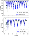Fig. B.1. Top:ΔP vs P diagram for the 0.5 M⊙ model in the fast rotating case. The asymptotic Lorentzian profile defined in Eq. B.74 are computed in the vicinity of the eigenfrequency of each inertial envelope mode. Bottom: Same as the top panel but for the 1 M⊙ model.

B.3.4. Frequencies in the inertial frame

The observed frequencies will be the ones from the inertial frame, ω_in = ω + mΩ = 2πν_in, and we can define the corresponding inertial period spacing, ΔP_in, as the period difference between two consecutive periods in the inertial frame. In Fig B.2, we show the ΔP_in versus ν_in diagram for both the 0.5 M_⊙ and the 1 M_⊙ models, in the three rotation regimes, slow, intermediate, and fast. First, we can note that the profile of the inertial dips is more pronounced in the case of the 0.5 M_⊙ model. The range of inertial frequency where the dips has to be searched also depends on the rotation regime, with the dips occurring at higher frequency for the fast rotating case (between 15 and 30 μHz), than for the intermediate (below 8 μHz) and slow (below 3 μHz) cases. While the low-frequency location of the first dip computed in the 0.5 M_⊙ slow case would make it challenging to characterise, the frequency range of the dip occurrence in the intermediate case should be much more easily accessible to observations granted that the temporal baseline is sufficient and the instrument is stable enough.

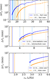Fig. B.2. Top:ΔPin vs νin diagram for the fast rotation case. The modes computed for the 0.5 M⊙ and 1 M⊙ models are represented in orange and blue, respectively, each dot corresponding to a mode. The eigenfrequencies of the envelope inertial modes are highlighted with the vertical dashed lines, in orange and light blue, respectively. For each model, the first and second harmonics of the rotation period are shown by the thick and dotted lines, respectively. Middle: Same as top panel for the intermediate rotation case. Bottom: Same as top panel for the slow rotation case.

It can finally be seen that the modes where the inertial dips occur are located between the first and second harmonics of rotation. Indeed, as expected from the relation between the inertial and co-rotation frequencies, for m = 1 modes, ω_in will asymptotically approach Ω as ω decreases (that is, as the mode absolute radial order increases). Around these harmonics, significant amplitude modulations from surface active regions can be expected. Nevertheless, if detectable, the signature from the gravito-inertial modes should be unambiguously distinguishable from the rotation peaks. Indeed, they are not located at the exact same frequency as the rotation peaks, and, more importantly, they will be asymmetrically distributed with respect to them, allowing for the characterisation of their regular pattern.

B.4. Numerical approach

B.4.1. Adimensioned equations

Oscillation equations are more conveniently numerically solved under an adimensioned formulation. By introducing the adimensioned coordinate x = r/R and the new variables y₁ and y₂ as defined by Townsend & Teitler (2013):

$$\begin{array}{cc}\hfill y_1& =\frac{{\xi }_r}{r}{x}^{2-\stackrel{\sim }{\ell }},\hfill \end{array}$$(B.76)

$$\begin{array}{cc}\hfill y_2& =\frac{p^{\prime }}{\rho gr}{x}^{2-\stackrel{\sim }{\ell }},\hfill \end{array}$$(B.77)

where g is the gravitational field, Eqs. 1 and 2 can be adimensioned, which yields

$$\begin{array}{cc}\hfill x{y}_{1}x& =[V_g-\stackrel{\sim }{\ell }-1-\frac{m\overline{\zeta }}{\overline{\omega }}]y_1+[\frac{\stackrel{\sim }{\ell }(\stackrel{\sim }{\ell }+1)}{C{\overline{\omega }}^2}-V_g]y_2,\hfill \end{array}$$(B.78)

$$\begin{array}{cc}\hfill x{y}_{2}x& =[C({\overline{\omega }}^2-2\overline{\mathrm{\Omega }}\overline{\zeta })-A^{\ast }]y_1+[A^{\ast }+m\frac{2\overline{\mathrm{\Omega }}}{\overline{\omega }}-\stackrel{\sim }{\ell }+3-U]y_2,\hfill \end{array}$$(B.79)

where (see Dziembowski 1971)

$$\begin{array}{cc}\hfill C& =x^3\frac{M}{M_r},\hfill \end{array}$$(B.80)

$$\begin{array}{cc}\hfill V_g& =-\frac{1}{{\mathrm{\Gamma }}_1}lnplnr=\frac{1}{{\mathrm{\Gamma }}_1}\frac{\rho gr}{p},\hfill \end{array}$$(B.81)

$$\begin{array}{cc}\hfill U& =\frac{4\pi \rho r^3}{M_r},\hfill \end{array}$$(B.82)

$$\begin{array}{cc}\hfill A^{\ast }& =\frac{N^{2}r}{g},\hfill \end{array}$$(B.83)

with M_r the mass contained within the sphere of radius r. The adimensioned frequencies $\overline{\omega }$, $\overline{\mathrm{\Omega }}$, and $\overline{\zeta }$ are defined as $\overline{\omega }(x)=\omega (x)/{\mathrm{\Omega }}_{\mathrm{c}}$, $\overline{\mathrm{\Omega }}(x)=\mathrm{\Omega }(x)/{\mathrm{\Omega }}_{\mathrm{c}}$, and $\overline{\zeta }(x)=\zeta (x)/{\mathrm{\Omega }}_{\mathrm{c}}$.

B.4.2. Boundary conditions

The boundary conditions we use are the following. First, we impose that the Lagrangian pressure perturbation, δp, vanishes at the surface of the star (x = 1),

$$\begin{array}{c}\hfill \delta p=p^{\prime }+{\xi }_{r}pr=0,\end{array}$$(B.84)

which translates to

$$\begin{array}{c}\hfill y_1(1)-y_2(1)=0.\end{array}$$(B.85)

Next, to regularise the problem at the centre of the star, we chose Ω to be a smooth profile that vanishes at x = 0:

$$\begin{array}{c}\hfill \mathrm{\Omega }(x)=(1-exp[-x/x_0]){\mathrm{\Omega }}_{★},\end{array}$$(B.86)

where we choose x₀ = 1  ×  10⁴. This way, given that for x → 0, A^* ∼ x³, V_g ∼ x², and U ∼ 3, the regularisation condition at the centre is

$$\begin{array}{c}\hfill C{\overline{\omega }}^2(0)y_1(0)-\stackrel{\sim }{\ell }{y}_2(0)=0.\end{array}$$(B.87)

Finally, we chose $\overline{\omega }(1)$ as the reference frequency to solve the system.

All Tables

All Figures

Fig. 1. Modulus of the squared Brunt-Väisälä frequency, |N2|, for the 0.5 M⊙ model (top) and the 1 M⊙ model (bottom). Regions where N2 ≥ 0 are in gray, and regions where N2 < 0 are in red. The squared Coriolis frequency, 4Ω2, is indicated by the horizontal dashed line for the slow (orange), the intermediate (yellow), and the fast (blue) cases, while the horizontal dotted lines correspond to 2Ω2. The propagation region of gravito-inertial waves as a function of frequency is highlighted by the hatched areas (orange dots and blue hatches for the slow and fast cases, respectively).

In the text

Fig. 2. Top: ΔP vs P diagram for the $\stackrel{\sim }{\ell }=m=1$ modes in the 0.5 M⊙ model in the co-rotating frame. The dots correspond to the modes computed considering the full extent of the stellar structure, with the slow case in orange, the intermediate case in yellow, and the fast case in blue. The vertical dashed lines mark the period of the modes computed considering only the convective envelope. The position of the Coriolis frequency, 2Ω, is highlighted for the slow, the intermediate, and the fast cases (vertical thick lines in orange, yellow, and blue, respectively), while the $\sqrt{2}\mathrm{\Omega }$ frequency is indicated with the vertical dotted lines. The location of the modes with the eigenfunctions represented in Fig. 3 is marked with the light blue stellar symbol. Bottom: Same as the top panel but for the 1 M⊙ model.

In the text

	Fig. 3. Comparison between the eigenfunctions of the n = −46 (orange) and n = −40 (dotted grey) modes. The eigenfunction of the n = −4 envelope mode is shown in dashed blue.
In the text

Fig. A.1. Evolutionary tracks for the stellar models (0.5 M⊙ in blue and 1 M⊙ in orange) considered in this work, from the end of the accreting phase to the ZAMS. The black thick lines shows the location of the ZAMS. The location on the track of the stellar models we consider in this work is highlighted by the star symbol. The other tracks of the Steindl et al. (2021) PMS grid ranging between M★ = 0.2 M⊙ and M★ = 1.5 M⊙ are shown in grey for comparison, with the structure model saved during the MESA run indicated by grey dots, yellow crosses, and teal plus signs. The crosses signal models which have a convective core while the plus signs correspond to stellar structure that are completely convective.

In the text

	Fig. A.2. Rotational evolution computed for the 0.5 (blue) and 1 M⊙ (orange) models. The rotational track with slow initial condition is represented with a dashed line, the track with intermediate initial condition with a dotted line, and the track with fast initial condition with a thick line. The location of the stellar models we consider in this work is highlighted by the star symbol.
In the text

	Fig. B.1. Top:ΔP vs P diagram for the 0.5 M⊙ model in the fast rotating case. The asymptotic Lorentzian profile defined in Eq. B.74 are computed in the vicinity of the eigenfrequency of each inertial envelope mode. Bottom: Same as the top panel but for the 1 M⊙ model.
In the text

Fig. B.2. Top:ΔPin vs νin diagram for the fast rotation case. The modes computed for the 0.5 M⊙ and 1 M⊙ models are represented in orange and blue, respectively, each dot corresponding to a mode. The eigenfrequencies of the envelope inertial modes are highlighted with the vertical dashed lines, in orange and light blue, respectively. For each model, the first and second harmonics of the rotation period are shown by the thick and dotted lines, respectively. Middle: Same as top panel for the intermediate rotation case. Bottom: Same as top panel for the slow rotation case.

In the text

References

- Aerts, C., Christensen-Dalsgaard, J., & Kurtz, D. W. 2010, Asteroseismology (Springer Science+Business Media B.V.) [Google Scholar]
- Alvan, L., Brun, A. S., & Mathis, S. 2014, A&A, 565, A42 [NASA ADS] [CrossRef] [EDP Sciences] [Google Scholar]
- Ando, H. 1985, PASJ, 37, 47 [NASA ADS] [Google Scholar]
- Augustson, K. C., Mathis, S., & Astoul, A. 2020, ApJ, 903, 90 [NASA ADS] [CrossRef] [Google Scholar]
- Barrault, L., Bugnet, L., Mathis, S., & Mombarg, J. S. G. 2025a, A&A, 701, A253 [NASA ADS] [CrossRef] [EDP Sciences] [Google Scholar]
- Barrault, L., Mathis, S., & Bugnet, L. 2025b, A&A, 694, A225 [NASA ADS] [CrossRef] [EDP Sciences] [Google Scholar]
- Bekki, Y., Cameron, R. H., & Gizon, L. 2022, A&A, 666, A135 [NASA ADS] [CrossRef] [EDP Sciences] [Google Scholar]
- Belkacem, K., Samadi, R., Goupil, M. J., et al. 2009, A&A, 494, 191 [NASA ADS] [CrossRef] [EDP Sciences] [Google Scholar]
- Borucki, W. J., Koch, D., Basri, G., et al. 2010, Science, 327, 977 [Google Scholar]
- Braginsky, S. I., & Roberts, P. H. 1995, Geophys. Astrophys. Fluid Dyn., 79, 1 [Google Scholar]
- Breton, S. N., Brun, A. S., & García, R. A. 2022, A&A, 667, A43 [NASA ADS] [CrossRef] [EDP Sciences] [Google Scholar]
- Cowling, T. G. 1941, MNRAS, 101, 367 [NASA ADS] [Google Scholar]
- Dziembowski, W. A. 1971, Acta Astron., 21, 289 [NASA ADS] [Google Scholar]
- Eggenberger, P., Buldgen, G., & Salmon, S. J. A. J. 2019, A&A, 626, L1 [NASA ADS] [CrossRef] [EDP Sciences] [Google Scholar]
- Fuentes, J. R., Barik, A., & Fuller, J. 2026, ApJ, 998, 131 [Google Scholar]
- Gallet, F., & Bouvier, J. 2015, A&A, 577, A98 [NASA ADS] [CrossRef] [EDP Sciences] [Google Scholar]
- Galoy, M., Lignières, F., & Ballot, J. 2024, A&A, 689, A177 [NASA ADS] [CrossRef] [EDP Sciences] [Google Scholar]
- Hanasoge, S. M. 2026, ApJ, 997, L22 [Google Scholar]
- Hindman, B. W., & Jain, R. 2022, ApJ, 932, 68 [NASA ADS] [CrossRef] [Google Scholar]
- Hindman, B. W., & Jain, R. 2023, ApJ, 943, 127 [Google Scholar]
- Howell, S. B., Sobeck, C., Haas, M., et al. 2014, PASP, 126, 398 [Google Scholar]
- Jain, R., & Hindman, B. W. 2023, ApJ, 958, 48 [Google Scholar]
- Jain, R., Hindman, B. W., & Blume, C. 2024, ApJ, 965, L8 [Google Scholar]
- Lantz, S. R. 1992, Ph.D. Thesis, Cornell University, United States [Google Scholar]
- Lecoanet, D., & Quataert, E. 2013, MNRAS, 430, 2363 [Google Scholar]
- Löptien, B., Gizon, L., Birch, A. C., et al. 2018, Nat. Astron., 2, 568 [Google Scholar]
- Mathis, S. 2009, A&A, 506, 811 [CrossRef] [EDP Sciences] [Google Scholar]
- Mathis, S., Neiner, C., & Tran Minh, N. 2014, A&A, 565, A47 [NASA ADS] [CrossRef] [EDP Sciences] [Google Scholar]
- Mathis, S., Breton, S., Dhouib, H., et al. 2023, A&A, submitted [Google Scholar]
- Matt, S. P., Brun, A. S., Baraffe, I., Bouvier, J., & Chabrier, G. 2015, ApJ, 799, L23 [Google Scholar]
- Matt, S. P., Brun, A. S., Baraffe, I., Bouvier, J., & Chabrier, G. 2019, ApJ, 870, L27 [Google Scholar]
- Messina, S., Catanzaro, G., Lanza, A. F., et al. 2024, A&A, 691, A117 [NASA ADS] [CrossRef] [EDP Sciences] [Google Scholar]
- Ouazzani, R. M., Lignières, F., Dupret, M. A., et al. 2020, A&A, 640, A49 [NASA ADS] [CrossRef] [EDP Sciences] [Google Scholar]
- Papaloizou, J., & Pringle, J. E. 1978, MNRAS, 182, 423 [NASA ADS] [CrossRef] [Google Scholar]
- Paxton, B., Bildsten, L., Dotter, A., et al. 2011, ApJS, 192, 3 [Google Scholar]
- Philidet, J., & Gizon, L. 2023, A&A, 673, A124 [NASA ADS] [CrossRef] [EDP Sciences] [Google Scholar]
- Pinçon, C., Belkacem, K., & Goupil, M. J. 2016, A&A, 588, A122 [NASA ADS] [CrossRef] [EDP Sciences] [Google Scholar]
- Press, W. H. 1981, ApJ, 245, 286 [Google Scholar]
- Press, W. H., Teukolsky, S. A., Vetterling, W. T., & Flannery, B. P. 1992, Numerical recipes in FORTRAN. The art of scientific computing (Cambridge: University Press) [Google Scholar]
- Rauer, H., Aerts, C., Cabrera, J., et al. 2025, Exp. Astron., 59, 26 [Google Scholar]
- Ricker, G. R., Winn, J. N., Vanderspek, R., et al. 2015, J. Astron. Telesc. Instrum. Syst., 1, 014003 [Google Scholar]
- Saio, H. 1982, ApJ, 256, 717 [Google Scholar]
- Saio, H., Takata, M., Lee, U., Li, G., & Van Reeth, T. 2021, MNRAS, 502, 5856 [Google Scholar]
- Skumanich, A. 1972, ApJ, 171, 565 [Google Scholar]
- Spada, F., Lanzafame, A. C., Lanza, A. F., Messina, S., & Collier Cameron, A. 2011, MNRAS, 416, 447 [NASA ADS] [Google Scholar]
- Steindl, T., Zwintz, K., Barnes, T. G., Müllner, M., & Vorobyov, E. I. 2021, A&A, 654, A36 [NASA ADS] [CrossRef] [EDP Sciences] [Google Scholar]
- Tassoul, M. 1980, ApJS, 43, 469 [Google Scholar]
- Tokuno, T., & Takata, M. 2022, MNRAS, 514, 4140 [NASA ADS] [CrossRef] [Google Scholar]
- Townsend, R. H. D. 2003, MNRAS, 340, 1020 [Google Scholar]
- Townsend, R. H. D., & Teitler, S. A. 2013, MNRAS, 435, 3406 [Google Scholar]
- Unno, W., Osaki, Y., Ando, H., Saio, H., & Shibahashi, H. 1989, Nonradial Oscillations of Stars (Tokyo: University of Tokyo) [Google Scholar]
- Weber, E. J., & Davis, L., Jr. 1967, ApJ, 148, 217 [Google Scholar]
- Zwintz, K., & Steindl, T. 2022, Front. Astron. Space Sci., 9, 914738 [NASA ADS] [CrossRef] [Google Scholar]
The code source is accessible at https://gitlab.com/sybreton/mascaret and the documentation at https://mascaret.readthedocs.io.
Unlike the case discussed in TT22, the two (pseudo-)turning points we consider here have the same nature and correspond to ω ∼ Neff.