| Issue |
A&A
Volume 708, April 2026
|
|
|---|---|---|
| Article Number | A229 | |
| Number of page(s) | 13 | |
| Section | Planets, planetary systems, and small bodies | |
| DOI | https://doi.org/10.1051/0004-6361/202348044 | |
| Published online | 08 April 2026 | |
Seasonal variation of the main gases in Titan's ionosphere from Cassini INMS data
1
LATMOS-IPSL’ CNRS, UVSQ, Université Paris-Saclay,
Guyancourt,
France
2
Max Planck Institute for Solar System Research,
Goettingen,
Germany
3
LESIA’ Observatoire de Paris, Université PSL, CNRS, Sorbonne Université, Université Paris-Cité,
Meudon,
France
4
Department of Earth and Planetary Sciences, Johns Hopkins University,
Baltimore,
MD,
USA
5
NASA Headquarters,
Washigton,
DC,
USA
6
NASA Goddard Space Flight Center,
Greenbelt,
MD,
USA
★ Corresponding author: This email address is being protected from spambots. You need JavaScript enabled to view it.
Received:
22
September
2023
Accepted:
29
January
2026
Abstract
With 13 years of observations, the Ion and Neutral Mass Spectrometer (INMS) on board the Cassini spacecraft has observed the upper atmosphere of Titan through two seasons: northern winter and spring. The complex atmosphere is mainly composed of N2, CH4, H2, and Ar, but many other carbon and nitrogen bearing trace species have been observed by INMS and other instruments. Using data from the closed source neutral (CSN) mode of the INMS instrument, we studied the abundance of the main gases and their variation in Titan’s ionosphere between 1500 and 950 km of altitude with a new mass spectra deconvolution code based on a Monte Carlo approach. Our results showed a hemispheric dichotomy in gas mole fractions at a constant altitude, with an enrichment of methane mole fraction in the southern hemisphere that seems to decreases after 2011 during northern spring. At constant N2 density, however, regardless of the hemisphere, we observe an increase in the N2 mole fraction with time. We note a strong correlation between the gas mole fraction and the solar cycle as well. We also derived an 14N/15N isotope ratio of 197.7 ± 3.9(3σ).
Key words: methods: data analysis / planets and satellites: atmospheres / planets and satellites: composition / planets and satellites: individual: titan
© The Authors 2026
 Open Access article, published by EDP Sciences, under the terms of the Creative Commons Attribution License (https://creativecommons.org/licenses/by/4.0), which permits unrestricted use, distribution, and reproduction in any medium, provided the original work is properly cited.
This article is published in open access under the Subscribe to Open model.
Open Access funding provided by Max Planck Society.
1 Introduction
The Cassini mission explored Saturn and its moons for 13 years, from 2004 to 2017. Before this mission, the probes Pioneer 11 and Voyager 1 & 2 flew by Titan and got the first closeup data (Tomasko 1980; Smith 1980; Tyler et al. 1981; Hartle et al. 1982; Lane et al. 1982). The other observations of Titan’s atmosphere came from ground and space-based telescopes with stellar occultations (Hörst (2017) and cited paper).
Cassini is the first spacecraft to get in situ data from Titan. The Ion and Neutral Mass Spectrometer (INMS) enabled many discoveries to be made about the ionosphere of Titan. We knew from previous observations that the main gases were N2, CH4, H2, and argon (Kuiper 1944; Smith et al. 1982; Owen 1982), but using INMS measurements the mole fraction could be determined with higher precision (Cui et al. 2009; Magee et al. 2009; Mandt et al. 2012; Cui et al. 2012, 2016). Trace species were also detected by this instrument (Cui et al. 2016), and together with the ion density (Cravens et al. 2006; Mandt et al. 2012) the results were used to improve the photochemical models of Titan atmosphere (Robertson et al. 2009; Vuitton et al. 2019). Indeed, methane and nitrogen are photo-dissociated in the atmosphere, and the recombination of these photoproducts creates a range of new species including gases (such as H2, HCN, C2H2, and C2H6) and aerosols.
The positive ion analysis of the instruments INMS and the Langmuir Probe also served to calculate the electron densities and the conductivity of the ionosphere. It was shown that the electron density and conductivity are lower during nighttime (Rosenqvist et al. 2009; Shebanits et al. 2017, 2022). Using models of hydrostatic equilibrium, Snowden et al. (2013) extracted thermal profiles of flybys through T72 from neutral data, obtaining mostly temperatures between 110 and 180 K depending on the flyby. They showed that extreme-ultraviolet (EUV) absorption is not the main determinant of the thermal structures of the thermosphere on a flyby timescale. Snowden et al. (2013) attributed the variations to magnetospheric particle precipitation. However, the temperature changes over a longer period of time could be correlated with EUV flux, as it also influences N2 and CH4 density (Westlake et al. 2014).
Saturn’s axial tilt allows Titan to have four seasons of approximately 7 Earth years each. During the mission, Cassini observed northern winter and spring. Westlake et al. (2014) reported the seasonal variation observed by INMS through 2013. In this paper, we study the entire Titan INMS inbound dataset in closed source neutral (CSN) mode up to the end of the mission in 2017 with the help of a new mass spectrometry data deconvolution code (Gautier et al. 2020) that overcomes some calibration uncertainties.
2 Method
2.1 INMS and mass spectrometry
INMS is a mass spectrometer that has different modes: it can analyse either the neutral species or cations, in open or closed source mode (Waite et al. 2004). In this paper, we analyse INMS data obtained in the CSN mode, which is better for the study of non-reactive neutral molecules (such as N2 and CH4). Neutral molecules are ionized and fragmented inside the INMS ionization chamber. The instrument counts for each atomic mass to charge ratio (m/z) the number of ions detected during the integration period (0.031032 s). Each molecule has a fragmentation pattern (FP) that depends on the molecule, its isotopes, and the instrumental transfer function specific to each mass spectrometer. With the INMS resolving power of 1 amu, multiple ions can have the same m/z ratio, and different molecules can have fragments in common. In an ideal case, the instrument will be well calibrated for all relevant species before going into space, which means we have all of the FP we need, with an error of <1%. That is rarely the case in reality, however. For INMS, ten relevant species for Titan were used to calibrate the instrument (Waite et al. 2004), which is sufficient for the scope of this paper. The spare unit that stayed on Earth was also used to complete some of the calibration data needed in other studies. When nothing else is available, another source of information is the National Institute of Standards and Technology (NIST) FP database, which is sparse in metadata and relevant information about the type of mass spectrometer used. All of these inconveniences complicate the deconvolution and interpretation of INMS mass spectra, as we aim to know which species contributed in what proportion to the mass peaks we observe.
2.2 Deconvolution code and data reduction
The uncertainty of the instrument transfer function and the FP is the reason why Gautier et al. (2020) developed a Monte Carlo approach to deconvolve these types of mass spectra. Once we built the FP database of species we expected to observe, we statistically explored the different databases possible within the allowed FP uncertainty. We deconvolved the signal for each randomly created FP database and selected the best 5% giving the most well-fitted spectra. We then retrieved the statistically most probable mole fractions of these species and averaged them. When looking for trace gases, the analysis of the results allowed us to determine if a species used in the database was indeed present, if its signature was overshadowed by another species, or if this species was in fact non-detected. That is why this process needed to be repeated as we adjusted the database of our selected expected species used in the deconvolution. We allowed an error of 5% on the FP for all gases (CH4, H2, and N2 in this study) except argon, for which we decided to allow an error of 30% because it was calibrated using Earth’s isotopic ratio. The mass spectra deconvolution code developed by Gautier et al. (2020) has been successfully applied by Serigano et al. (2020, 2022) to analyse Saturn INMS data, Leseigneur et al. (2022) for Rosetta data, and Gautier et al. (2024); Das et al. (2025) for Huygens Gas Chromatograph/Mass Spectrometer (GC/MS) data.
We re-calibrated INMS data by taking into account the dead time correction, the ram pressure enhancement, the saturation correction, the sensitivity, and the contamination by thruster firing following procedures detailed in Cui et al. (2009, 2012); Magee et al. (2009); Teolis et al. (2015). We decided to focus our analysis on the ingress part of the signal (also called ‘inbound data’) to avoid the wall adsorption effect whereby adsorbed molecules can be released later by the walls, modifying the molecular densities and the mole fractions. To retrieve the molecular mole fractions, we used a Monte Carlo sampling on the FP to deconvolve the signal. For each scan sequence, INMS analysed 68 masses, one at a time and not in order. Some masses were analysed twice or more during the sequence, and some others were not analysed at all. To obtain a complete mass spectrum (m/z 1 to 99), we stacked INMS data over two sequences, which increased the uncertainty in the altitude, and averaged over the number of actual numerical stacked values.
We decided for now to include only the FP of four main gases in our database: molecular nitrogen and hydrogen, methane, and argon. Thankfully we do have an INMS FP for these species. We acknowledge that there is a slight bias in our mole fractions as we do not account for trace species in Titan atmosphere, but they are negligible compared to N2 and CH4 mole fractions. We only selected flybys going below 1500 km in altitude as this is where we start to have a solid signal of N2.
3 Results
In Table A.1 is the list and details of the flybys used in our analysis, together with the temperatures extracted from Eq. (3). in Section 4.1.
3.1 Densities
Extracting the densities can be tricky, as we need the neutral temperature profile. But to calculate it we need the density. Snowden et al. (2013) calculated the temperature profiles for a few flybys using models fitted to INMS data. To ease our task, we decided to test the hypothesis of a constant temperature profile (150 K later in the study). We retrieved N2 densities using the following formula from Teolis et al. (2015):
 (1)
(1)
with nf being the density of species f, Xf the detector count rate for species f, T0=293 K the temperature during the calibration process, and Ta the ambient temperature of the gas. Sf is the sensitivity of the gas and DSf the ram pressure enhancement (Teolis et al. 2015) that also depends on Ta. The ram pressure is the pressure at the front of the spacecraft caused by its entrance into the atmosphere, which can enhance the signal and has to be taken into account. To check the relevance and impact of this hypothesis on our results, we calculated N2 densities for all flybys at two different constant profiles of Ta, at 100 K and 200 K, chosen from extreme values retrieved by Snowden et al. (2013). The percentage difference between these two results is presented in Fig. 1. As DSf varies with Ta, we cannot say that the observed difference is a factor depending on  . However, as was expected with Eq. (1), the density decreases when the ambient temperature increases. The absolute difference in our results is mostly between 0.1 and 0.5%, which is way below our error bars due to the calibration process. This result means that even a temperature variation of 100 K would not significantly change the densities retrieved in this work.
On the right part of Fig. 1, we can distinguish the flyby by colour. We can follow the progressive evolution of the molecular density depending on the date of the flyby. Thanks to the left and middle part of the figure, we can infer that the variations we observe are not related to the chosen temperature profile in Eq. (1). A phenomenon different from temperature changes could be the source of these variations. For the rest of our study, we kept a temperature profile of 150K, which is a good compromise between the lowest and highest values of retrieved temperatures by Snowden et al. (2013).
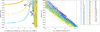 |
Fig. 1 (Left) Percentage of differences between the retrieved N2 densities of flybys from Table A.1 using a temperature profile of 100 and 200 K. With a few exceptions, the difference is below 0.5%. Flybys T96, T97, T105, and T109 reach 30% of difference. (Right) N2 retrieved densities for all flybys for a constant T profile of 150 K. The colours depend on the flyby, and the density points are stacked and averaged. |
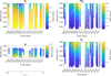 |
Fig. 2 Vertical profiles of N2, CH4, Ar, and H2 mole fractions through time (filled squares). Note that all colour scales are linear except for H2. Mole fractions from flyby T64 (filled diamonds) come from Westlake et al. (2014).The solar longitude is indicated below the left graphs, with relevant longitudes corresponding to the years above. By convention the northern spring equinox corresponds to the solar longitude Ls = 0°. |
3.2 Mole fraction
We calculated the mole fractions of the main gases for all flybys from Table A.1. Our results in Fig. 2 show a strong variation over time, which was also observed by Westlake et al. (2014) on the neutral species. As the altitude increases, so does the CH4 and H2 mole fraction. On the contrary, heavier gases such as N2 and Ar have a mole fraction that decreases when the altitude increases. This is evidence towards the presence of a homopause, whereby Titan’s upper atmosphere starts to have a segregation of species depending on their molecular masses, and beyond which the molecular diffusion starts to become dominant as the altitude increases. This phenomenon is known as diffusive separation. The homopause altitude also varies over time as is discussed in Section 4.1.
3.2.1 N2
N2 is the most abundant gas in Titan’s atmosphere. Below 1250 km, counter 1 of INMS starts to saturate at m/z 28 because of the increasing molecular density of 14N14N. Therefore we need to switch to data from the low-sensitivity counter 2. We also used Cui et al. (2012)’s method to correct part of the saturation data before completely switching to using data from counter 2.
We did not separate the different isotopes in our analysis. The FP we used took into account both 14N14N and 15N14N as a single species with fragments at m/z 14, 15, 28, 29, and 30. Our model selects the FP database with the smallest fit residue taking all altitudes into account. That does not allow for a change in the isotope ratio with altitude as the final database is the same for all altitudes. We may hence have a slight bias in our retrieved isotope ratio. However, based on the parts of the signal due to N2 at the different masses, we obtained a 14N/15N isotope ratio of 197.7 ± 3.9(3σ) when fitting a Gaussian on the isotope ratio distribution histogram. We calculated the isotopic ratio following this equation:
 (2)
(2)
with XN the count/s due to nitrogen at m/z 14 or 15 reconstituted with the deconvolution code. Our result is in agreement with Niemann et al. (2005), Waite et al. (2005), Mandt et al. (2009), and Cui et al. (2012) (14N/15N = 200-220, 160-260, 183 ± 5, and 172-215, respectively). Using the curve fitting method described in the Figure 14 of Niemann et al. (2010), we obtained 14N/15N = 202.6±0.3 which is higher than their value (167.6±0.6) using the GC/MS on board Huygens below 140 km of altitude. When calculating these values we excluded flybys T88, T96, and T97 because the only masses analysed were m/z 2, 16, and 28.
3.2.2 CH4
Methane is the second major gas in Titan’s atmosphere. There is still an ongoing mystery surrounding the source of methane in the atmosphere. Without renewal, atmospheric methane should be depleted in a few tens of millions of years (Tobie et al. 2006) because of the photo-dissociation of the molecule and the recombination into different hydrocarbons. It means that either there is a continuous source of methane replenishing the atmosphere, or there are multiple events doing it. One of the possibilities is the presence of methane clathrate in the icy crust (Tobie et al. 2006; Choukroun et al. 2010). It can be released when the ice melts after a meteoric impact. The presence of alkanofers containing liquid hydrocarbons, similar to the aquifers on Earth, is also possible (Hayes et al. 2008). In Fig. 2, we clearly observe an increase in the proportion of methane in the atmospheric mix above 1300-1400 km of altitude between 2007 and 2010, going from 2-6% to 20-35%. Methane (16 amu) is lighter than molecular nitrogen (28 amu), which means that above the homopause its mole fraction will increase compared to heavier gases. It can also escape from the atmosphere more easily (Yelle et al. 2008; Strobel 2009; Bell et al. 2011; Cui et al. 2012).
3.2.3 Argon
While the primordial argon isotope is at m/z 36, the radiogenic isotope issued from the disintegration of 40K peaks at m/z 40. On Jupiter, the primordial isotope is the most abundant, while on Earth, due to the mantle and crust containing 40K, the most abundant isotope is 40Ar. This is also the case on Titan, giving information on the rocky part of the satellite. In this way, Tobie et al. (2012) showed that a chondritic composition is enough to provide previously found abundances of 40Ar and 36Ar (Niemann et al. 2010) in Titan’s atmosphere. This is proof that there are exchanges between the interior and the atmosphere of Titan. INMS was calibrated using Earth’s isotope ratio, which may not be the same as Titan’s. We decided to allow an uncertainty of 30% for Argon FP at m/z 20, 36, and 40 because of this. While m/z 40 is still the main peak of Ar, other gases such as CH3C2H and C3H6 also contribute to m/z 40, even if their contributions are more relevant in outbound data (not included in our analysis) due to wall adsorption (Cui et al. 2012). Argon can be reliably detected below 1150 km of altitude, but we do start to see a signal at m/z 40 below 1300 km, and below 1150 km for m/z 36, depending on the flyby.
Niemann et al. (2010) measured with the GC/MS a mole fraction of (3.35±0.25).10−5 for 40Ar from 18 km to the surface of Titan. This is within the range of some of our results at the lowest altitudes with INMS (Fig. 2-Ar, but overall we tend to obtain higher values of between 4 and 5.10−5. Yelle et al. (2008) and Cui et al. (2012) also obtained lower values after removing contribution from other trace species, which we did not do in this study as the scope was the main gases. Another study focusing on the trace gases using the same method of mass spectra deconvolution is needed to properly investigate the argon. For the argon we will concentrate more on the variations than the actual value of the mole fraction as the bias is systematic. The mole fractions of Argon follow N2 variations’ tendencies flyby to flyby and also decrease as the altitude increases. Contrary to the other species, INMS cannot probe the atmosphere deeply enough to observe a constant mole fraction before it varies with the altitude.
3.2.4 H2
INMS used a quadrupole mass analyser (QMS), which is usually not the best for the measurement of H2 . Indeed, this molecule reacts with the filament of the QMS. It is also subject to rapid diffusion, because the molecule is small and light, affecting its pumping efficiency in the system. Furthermore, the radio-frequency field needs to be extremely high and steady to constrain measurements at m/z 1 (fragmentation of H2), which means that we may measure m/z 1 and heavier species at the same time if these conditions are not respected. While the calibration of the instrument helps in solving part of the problem, it does not completely go away, so our results for this molecule have to be taken with caution. Strobel (2022) also questioned the INMS calibration at low masses and showed that the corrective enhancement factor added in Teolis et al. (2015) may not be necessary for H2.
On Titan, H2 comes from the UV photodissociation of CH4, directly or by recombination of molecular hydrogen (Yung et al. 1984; Lebonnois et al. 2003). It was likely not present in Titan’s primordial atmosphere. We observe an exponential increase in the H2 mole fraction at high altitude in Fig. 2. The colour scale is exponential for this plot, allowing us to see the stability at low altitude and fast changes at high altitude, where the mole fraction value is increased by more than a factor of 10, which is a greater factor than that of all other main gases. These results are expected as H2 is the lightest gas. Above the homopause where molecular diffusion dominates, H2 will rise higher than all the other gases, so mathematically its mole fraction also increases significantly. The H2 abundance below the homopause is between 0.4 and 1%, which is already ten times higher than the values from the stratosphere and troposphere (Niemann et al. 2010), and in agreement with Waite et al. (2005) and Cui et al. (2009).
4 Discussion
4.1 Homopause
The homopause is defined at a level where the eddy diffusion and the molecular diffusion are equal to each other. The determination of the homopause altitude on Titan has been greatly discussed in previous studies (Waite et al. 2005; Yelle et al. 2008; Mandt et al. 2009; Cui et al. 2009; Strobel 2009; Bell et al. 2011; Cui et al. 2012). While Waite et al. (2005) found an altitude of 1195 ± 65 km using the intersection between the eddy coefficient and the N2-CH4 diffusion coefficient profiles, Yelle et al. (2008) found a lower altitude of 850 km for 40 Ar with their model. Bell et al. (2011) found a methane homopause at roughly 1000 km. Cui et al. (2012) contested their results and obtained values under 900 km using 40Ar. A comparison between the Cassini Ultraviolet Imaging Spectrograph (UVIS), Cassini Attitude and Articulation Control Subsystem (AACS), Huygens Atmospheric Structure Instrument (HASI), and INMS (Koskinen et al. 2011; Strobel 2010) detected the need of a factor of 2.6-3.2 between INMS retrieved densities and densities retrieved with the other instruments. Later, Teolis et al. (2015) demonstrated the origin of this factor, related to the ram pressure enhancement and the instrument orientation during the flyby.
Except for Cui et al. (2012) and Bell et al. (2011), these studies did not take the factor of 3 for INMS densities into account, which may result in a shift for the altitudes retrieved by the models using INMS data to be fitted. Bell et al. (2011), Yelle et al. (2008), and Cui et al. (2012) also used INMS data averaged from the T1 to T40 or T71 flybys, which means that they cannot observe a seasonal shift in the homopause altitude. For most of these studies, the homopause altitude retrieved by the diffusion models is below the altitude probed by INMS, but not for all of them. We chose a different approach to estimate the homopause altitude, based only on INMS results of N2 and not on diffusion models and 40 Ar. Above the homopause, the molecular density, n (cm−3), of the gases decreases at a rate that depends on their masses. It should follow the exponential equation
 (3)
(3)
with the scale height
 (4)
(4)
with z (m) the altitude, n0 the molecular density at the surface, MG (g/mol) the molecular mass of a gas, G, or air, T, (K) the mean temperature of the atmospheric layer, R (kg.m2.s−2 K−1 mol−1) the gas constant, and g (m s−2) the acceleration due to gravity (here g = 0.84 m s−2 at 1200 km of altitude). It means that on a graph (z,n) with a log-scale on the ordinate, a break of slope indicates either the position of the homopause, a chemical reaction in the atmosphere that changes the density of N2, or an atmospheric wave. For each flyby we fitted two exponential curves corresponding to these slopes.
The first curve (in blue on Fig. 3) takes into account the points at higher altitude until a break in the slope is observed, and the second curve (in red) fits the molecular density at lower altitude, after the observed break in the slope. We hypothesize that the altitude of the homopause starts when the first curve does not fit the data any more. As the altitude of the homopause seen in Fig. 3 is often where we have to change counter due to saturation, we decided to do the same for 14N15N density using mass 29 (dashed lines). The extracted temperatures using Eq. (3) are similar for both densities, which provides confidence in our fits (see Table A.1). The vertical lines signal the altitudes below which N2 data points (and its isotope) can no longer be fitted by the blue curves. We presented in Fig. 3 different cases: (a, c, d) have slower decreases in molecular density above the homopause, contrary to (b) where the blue lines are steeper. We can also observe wave-like patterns in (a) and (c) below 1200 km of altitude as the data points oscillate around the red lines.
Atmospheric waves occur in Titan’s ionosphere and are observed either in the temperature profiles or in the molecular density profiles (Fulchignoni et al. 2005; Koskinen et al. 2011; Müller-Wodarg et al. 2006; Snowden et al. 2013; Cui et al. 2014). The observed vertical wavelength is between 150 and 400 km (Snowden et al. 2013; Cui et al. 2014). If the changes of slope we observed (vertical lines) were due to an atmospheric wave, the wavelength would be greater than 700 km (from Fig. 3), which is not what was observed previously. This is why we infer that the changes in slope that we noted with vertical lines are due to the nitrogen homopause.
Argon is less sensitive to photochemistry, which is why Yelle et al. (2008) and Cui et al. (2012) used only argon to constrain the eddy mixing profile used in their diffusive equilibrium model, compared to Bell et al. (2011) who used 14N15N and 40Ar density data. When we looked at the 40Ar molecular density, there was no break of slope when fitting the data with Eq. (3) (see Fig. B.2 of the appendix). That means that for argon the homopause is lower than the probing depth of INMS, which is consistent with the results of Yelle et al. (2008); Cui et al. (2012). Moreover, the argon mixing ratio is not constrained as well as the nitrogen in our retrievals at high altitudes, which means that any break in the slope potentially detected would have high uncertainties.
As a consequence of the domination of molecular diffusion, the mole fractions of the gases also change. However, as argon is only up to 0.005% of the mole fraction at the probed altitudes, its impact on the mole fractions of the other main gases is negligible. This is why, to complement our previous results using molecular density, we decided to check the evolution of N2 mole fraction as we feel it is more representative, making the same assumption that a change of slope is indicative of the homopause or a chemical reaction. Like the previous method, we fitted the mole fractions points at lower and higher altitude with different linear fits, and marked the positions where the data could not be fitted any more. The area between the two fits was interpreted as a transition zone between the two different diffusion regimens. The detailed results are in the appendix. We take the progressive transition and segregation of the species with the altitude into account. INMS data also do not give us a vertical profile at constant longitude and latitude, which means we could have differences caused by horizontal pressure variation, impacting the mole fractions and molecular densities. These are the reasons why we delimited a grey area of transition as the homopause for each flyby on Fig. 4 using the results of our different methods. We note that the lower limit altitude tends to decrease over the years. Our results using N2 are more in agreement with Waite et al. (2005) and Bell et al. (2011) CH4 homopause, even if the former did not take the factor of 3 into account. Seeing the intense variability that we observe on the densities, we can question the method of averaging the results over so many flybys to apply the diffusion model, instead of averaging over 2-Earth-year periods for example, taking into account the seasonal variations.
We cannot exclude the possibility that the changes we observe in the mole fraction and molecular density are partially due to chemical reactions at 1100-1250 km, as previous studies located the homopause around 840 km. Vuitton et al. (2019) calculated the photo-dissociation rate of N2, increasing from 1500 to 1140 km before decreasing again. We could thus expect a steeper slope below 1140 km, but that is not the case for all flybys, as is shown in Fig. 3 by the reversed relative positions of the blue and red fitting lines on flyby T27 compared to T87, meaning that the chemistry is not the only factor changing the slope of the molecular nitrogen density.
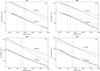 |
Fig. 3 N2 molecular density for flybys T5, T27, T30, and T87. The top data points, fitted with plain lines, are the averaged molecular density of 14N 14N stacked over four data points. The bottom data points, fitted with dashed lines, are for 14N 15N molecular density. In blue and red are the fitted lines using equation 3 at high and low altitude, respectively, for 14N14N (plain) and 14N15N (dashed). The vertical lines are the altitudes below which 14N14N (plain) and 14N15N (dashed) data point cannot be fitted anymore by the blue curve. |
4.2 Hemispheric dichotomy and seasonal variation
We observe a hemispherical dichotomy between the two hemispheres for the N2 and CH4 mole fractions. At a constant altitude (Fig. 5 left), it seems that the N2 mole fraction is higher in the northern hemisphere. It is, however, difficult to determine if there is a seasonal inversion of this phenomena as the flybys did not alternate between the northern and southern hemispheres but focused mainly on one hemisphere in each mission (Prime, Equinox, and Solstice), and we have a nearly two-year break between July 2010 and May 2012 with no flybys. If these observations were due to the Hadley circulation cell that goes downwards at the north pole and upwards at the south pole before the vernal equinox, we should expect a progressive inversion of this circulation until completion around the summer solstice (Vinatier et al. 2015; Mathé et al. 2020). We do observe after 2012 an increase in the N2 mole fraction in the southern hemisphere that tends to confirm this expectation, but we do not observe a significant decrease in the northern N2 mole fraction except for flyby T126. Similarly to Müller-Wodarg et al. (2008), we note an increase in the CH4 mole fraction in the northern polar latitude (inferred by the decrease of N2 mole fraction in the figure), partially due to the thinner atmosphere at the pole, meaning that for the same altitude we probe at a lower pressure. These differences disappear when we compare the mole fraction at a constant N2 molecular density instead of a constant altitude (Fig. 5 right).
When looking at the mole fraction at a constant N2 density, the results are a bit different. We observe a temporal dichotomy: before 2010, most of the flybys’ N2 mole fractions are between 0.85 and 0.92 regardless of the hemisphere, and after 2012 the N2 mole fractions are between 0.9 and 0.95. This means that for the same N2 density, the CH4 density relatively decreases after the vernal equinox globally on Titan. It means that there is a mechanism that either reduces methane densities or increases molecular nitrogen densities on a global scale, independently of the changes in atmospheric circulation due to seasonal changes.
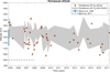 |
Fig. 4 Upper and lower limits of the transition area between the homosphere and the heterosphere for each flyby from the mole fraction (grey) and the molecular density (red) of N2. The results from Waite et al. (2005) are in blue and those from Bell et al. (2011) are represented by the dashed grey line. |
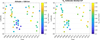 |
Fig. 5 N2 mole fraction as a function of latitude and time, at a constant altitude of 1300 km (left) and at a constant molecular density of 108 (right). |
4.3 Solar EUV
Similarly to Westlake et al. (2014), we note a strong correlation between the N2-CH4 mole fractions observed and solar activity. They observed a drop in CH4 mole fraction at constant N2 density during the rising phase of the solar cycle, when the emitted solar flux starts to increases. We plotted N2 molecular density and mole fraction as a function of time, superimposed with the solar 10.7 F cm flux1 in Fig. 6. We notice that the correlation is two-fold. First, the molecular densities (both N2 and CH4) increase when solar flares happen. This could be explained by the compression of Titan’s atmosphere when the coronal mass ejection (CME) reaches the satellite, which means that for the same altitude, the neutral density increases during a flare. However, the N2 mole fraction increases nonetheless, which means that there is also more photo-dissociation of CH4. Secondly, on a solar cycle timescale, N2 mole fraction follows the rise and fall of solar flux, for the same reasons.
Westlake et al. (2014) proved that the changes observed were related to the solar cycle and not the seasonal variation by comparing these results with Voyager observations. Nonetheless, the EUV influence is also affected by the distance from the Sun. The perihelion (9.03 AU) of Saturn’s orbit occurs at the beginning of Titan’s northern winter (2003), while the aphelion (10.04 AU) happens after the summer solstice (2017, see the solar longitude timescale in Fig. 2 for visual help). It means that Titan is closer to the sun during northern winter. This can explain why, while the solar activity was weaker during the prime mission in winter, its impact is greater than during spring (for an equivalent solar activity), as we can see in Fig. 6.
On a short timescale, the variations in the homopause altitude also follow the solar activity, but over a longer period of time, the altitude tends to slightly decreases, due to the increasing distance from the Sun. While the analysis of the ion and electron densities shows a clear difference between the day-side and the night-side (Rosenqvist et al. 2009; Shebanits et al. 2017, 2022), it is less evident with neutral species. We were unable to establish a clear difference or similarity in the mole fraction between the night-side and day-side for flybys at the same location on a short timescale (of less than 6 months) as we did not have enough flyby respecting these constraints. According to the species having a longer photochemical timescale than the horizontal mixing timescale, we should expect no differences in the mole fraction between the day and night sides in Titan’s atmosphere anyway.
 |
Fig. 6 Solar F10.7 cm radio flux over N2 mole fractions (left) and N2 density profiles (right). |
5 Conclusion
Solar EUV is the major driving force behind long-term variations in the main neutral species in Titan’s ionosphere. We observed a correlation between the solar cycle and the mole fractions of molecular nitrogen and methane, showing an increase in CH4 photo-dissociation as the solar cycle entered its rising phase. However its impact is lessened by the increasing distance between the Sun and Saturn from 9 to 10 AU over the course of the mission. We noticed that during northern winter, less solar flux is needed to increase the N2 mole fraction compared to the end of the mission. On a shorter timescale, the peaks observed in all mole fractions correlated with the solar flares seem to be due to the compression of the atmosphere once the solar CME reaches the moon. Neutral species mole fractions do not seem to be affected by the shift from day to night, but we did not have enough flybys close in space and time taken on the day and night sides to draw a firm conclusion. We calculated the homopause altitude for 51 flybys based on the retrieved densities and mole fraction of N2, and showed that its altitude is also impacted by solar EUV, but tends to decreases as the season shifts to summer and the distance with the Sun increases. The mean lower boundary of the transition zone of the homopause seems to be around 1150 km, which is in disagreement with most of the previous studies using diffusion models fitted over INMS data. At constant altitude, the southern hemisphere is enriched in CH4 until at least 2011. The next southern data after 2016 seems to show a decrease in this enrichment. At a constant density, we observed a clear temporal dichotomy, with a clear decrease in the CH4 mole fraction after 2012 in both hemispheres. These results are indicative of both the changes in atmospheric circulation due to the seasonal variation, and the increase in solar EUV after 2012.
The Dragonfly mission is expected to land in the mid-2030s during northern winter, as Huygens did 30 years before. It is too soon to rely on the solar activity forecast for 2034 because, depending on the Space Weather Prediction Center website or the models, the solar cycle activity will either be low or on the rise (Benson et al. 2020; Herrera et al. 2021). This difference can change the column density by a factor of up to 5 at altitudes between 1000 to 1500 km. This may be a point to take into account for the braking phase of Dragonfly when entering the atmosphere, as it could potentially affect the landing site position inside the calculated landing ellipse.
On flyby T96, Titan was outside of Saturn’s magnetosphere when a strong CME reached the moon (Bertucci et al. 2015). The N2 density had increased by a factor of 3 compared to flybys T92 and T97 - whose solar activity was, respectively, lower and higher during the flybys. The position of Titan with respect to Saturn’s magnetosphere may need to be taken into account in case of a solar event occurring up to a week before the Dragonfly landing.
INMS temporal sampling was not enough to precisely follow the ionosphere and thermosphere reaction to solar flux, CME, Saturn’s magnetosphere, season, latitude, and time of day. A new Titan-focused spacecraft equipped with a mass spectrometer and instruments that measure the EUV flux and Saturn’s magnetic field, a high-resolution RADAR, and an IR and UV spectrometer could enable Titan’s surface and complex atmosphere to be studied for a full Saturnian year.
Data availability
All retrieved data are available in the Zenodo repository https://doi.org/10.5281/zenodo.18460051
Acknowledgements
We also extend our thanks and acknowledgement to the following programs who funded us throughout this work: the Programme National de Planétologie (PNP) of CNRS/INSU co-funded by CNES; the Agence Nationale de la Recherche under the grant ANR-20-CE49-0004-01 to M.C., T.G. and K.D.; the NASA Cassini Data Analysis Program under CDAP16 2-0087 to T.G., J.S and S.M.H. and the NASA Cassini Data Analysis Program Grants 80NSSC19K0903 to J.S. and S.M.H.
References
- Bell, J. M., Bougher, S. W., Waite Jr, J. H., et al. 2011, J. Geophys. Res. Planets, 116 [Google Scholar]
- Benson, B., Pan, W., Prasad, A., Gary, G., & Hu, Q. 2020, Sol. Phys., 295, 65 [Google Scholar]
- Bertucci, C., Hamilton, D., Kurth, W., et al. 2015, Geophys. Res. Lett., 42, 193 [Google Scholar]
- Choukroun, M., Grasset, O., Tobie, G., & Sotin, C. 2010, Icarus, 205, 581 [Google Scholar]
- Cravens, T. E., Robertson, I. P., Waite, J. H., et al. 2006, Geophys. Res. Lett., 33, 8 [Google Scholar]
- Cui, J., Yelle, R. V., Vuitton, V., et al. 2009, Icarus, 200, 581 [NASA ADS] [CrossRef] [Google Scholar]
- Cui, J., Yelle, R. V., Strobel, D. F., et al. 2012, J. Geophys. Res. E: Planets, 117, 1 [Google Scholar]
- Cui, J., Yelle, R., Li, T., Snowden, D. F., & Müller-Wodarg, I. 2014, J. Geophys. Res.: Space Phys., 119, 490 [Google Scholar]
- Cui, J., Cao, Y.-T., Lavvas, P. P., & Koskinen, T. T. 2016, ApJ, 826, L5 [Google Scholar]
- Das, K., Gautier, T., Szopa, C., et al. 2025, A&A, 700, A86 [NASA ADS] [CrossRef] [EDP Sciences] [Google Scholar]
- Fulchignoni, M., Ferri, F., Angrilli, F., et al. 2005, Nature, 438, 785 [CrossRef] [Google Scholar]
- Gautier, T., Serigano, J., Bourgalais, J., Hörst, S. M., & Trainer, M. G. 2020, Rapid Commun. Mass Spectrom., 34, 1 [Google Scholar]
- Gautier, T., Serigano, J., Das, K., et al. 2024, A&A, 690, A165 [NASA ADS] [CrossRef] [EDP Sciences] [Google Scholar]
- Hartle, R., Sittler Jr, E., Ogilvie, K., et al. 1982, J. Geophys. Res.: Space Phys., 87, 1383 [Google Scholar]
- Hayes, A., Aharonson, O., Callahan, P., et al. 2008, Geophys. Res. Lett., 35 [Google Scholar]
- Herrera, V. V., Soon, W., & Legates, D. 2021, Adv. Space Res., 68, 1485 [Google Scholar]
- Hörst, S. M. 2017, J. Geophys. Res.: Planets, 122, 432 [CrossRef] [Google Scholar]
- Koskinen, T., Yelle, R., Snowden, D., et al. 2011, Icarus, 216, 507 [CrossRef] [Google Scholar]
- Kuiper, G. P. 1944, ApJ, 100, 378 [NASA ADS] [CrossRef] [Google Scholar]
- Lane, A. L., Hord, C. W., West, R. A., et al. 1982, Science, 215, 537 [NASA ADS] [CrossRef] [Google Scholar]
- Lebonnois, S., Bakes, E. L., & McKay, C. P. 2003, Icarus, 161, 474 [NASA ADS] [CrossRef] [Google Scholar]
- Leseigneur, G., Bredehöft, J. H., Gautier, T., et al. 2022, Angew. Chem. Int. Ed., 61, e202201925 [Google Scholar]
- Magee, B. A., Waite, J. H., Mandt, K. E., et al. 2009, Planet. Space Sci., 57, 1895 [NASA ADS] [CrossRef] [Google Scholar]
- Mandt, K. E., Waite, J. H., Lewis, W., et al. 2009, Planet. Space Sci., 57, 1917 [Google Scholar]
- Mandt, K. E., Gell, D. A., Perry, M., et al. 2012, J. Geophys. Res. Planets, 117, 1 [Google Scholar]
- Mathé, C., Vinatier, S., Bézard, B., et al. 2020, Icarus, 344, 113547 [CrossRef] [Google Scholar]
- Müller-Wodarg, I., Yelle, R., Borggren, N., & Waite Jr, J. 2006, J. Geophys. Res.: Space Phys., 111, A12 [CrossRef] [Google Scholar]
- Müller-Wodarg, I. C., Yelle, R. V., Cui, J., & Waite, J. H. 2008, J. Geophys. Res.: Planets, 113, 1 [Google Scholar]
- Niemann, H., Atreya, S., Bauer, S., et al. 2005, Nature, 438, 779 [CrossRef] [Google Scholar]
- Niemann, H. B., Atreya, S. K., Demick, J., et al. 2010, J. Geophys. Res.: Planets, 115 [Google Scholar]
- Owen, T. 1982, Planet. Space Sci., 30, 833 [Google Scholar]
- Robertson, I. P., Cravens, T. E., Waite, J. H., et al. 2009, Planet. Space Sci., 57, 1834 [NASA ADS] [CrossRef] [Google Scholar]
- Rosenqvist, L., Wahlund, J. E., Âgren, K., et al. 2009, Planet. Space Sci., 57, 1828 [Google Scholar]
- Serigano, J., Hörst, S. M., He, C., et al. 2020, J. Geophys. Res.: Planets, 125, 1 [Google Scholar]
- Serigano, J., Hörst, S., He, C., et al. 2022, J. Geophys. Res.: Planets, 127, e2022JE007238 [Google Scholar]
- Shebanits, O., Vigren, E., Wahlund, J. E., et al. 2017, J. Geophys. Res.: Space Phys., 122, 7491 [Google Scholar]
- Shebanits, O., Wahlund, J. E., Waite, J. H., & Dougherty, M. K. 2022, J. Geophys. Res.: Space Phys., 127, 1 [CrossRef] [Google Scholar]
- Smith, P. H. 1980, J. Geophys. Res. Space Phys., 85, 5943 [Google Scholar]
- Smith, G. R., Strobel, D. F., Broadfoot, A., et al. 1982, J. Geophys. Res.: Space Phys., 87, 1351 [Google Scholar]
- Snowden, D., Yelle, R. V., Cui, J., et al. 2013, Icarus, 226, 552 [Google Scholar]
- Strobel, D. F. 2009, Icarus, 202, 632 [Google Scholar]
- Strobel, D. F. 2010, Icarus, 208, 878 [Google Scholar]
- Strobel, D. F. 2022, Icarus, 376, 114876 [Google Scholar]
- Teolis, B. D., Niemann, H. B., Waite, J. H., et al. 2015, Space Sci. Rev., 190, 47 [Google Scholar]
- Tobie, G., Lunine, J. I., & Sotin, C. 2006, Nature, 440, 61 [Google Scholar]
- Tobie, G., Gautier, D., & Hersant, F. 2012, ApJ, 752, 125 [Google Scholar]
- Tomasko, M. 1980, J. Geophys. Res. Space Phys., 85, 5937 [Google Scholar]
- Tyler, G., Eshleman, V., Anderson, J., et al. 1981, Science, 212, 201 [NASA ADS] [CrossRef] [Google Scholar]
- Vinatier, S., Bézard, B., Lebonnois, S., et al. 2015, Icarus, 250, 95 [NASA ADS] [CrossRef] [Google Scholar]
- Vuitton, V., Yelle, R. V., Klippenstein, S. J., Hörst, S. M., & Lavvas, P. 2019, Icarus, 324, 120 [CrossRef] [Google Scholar]
- Waite, J. H., Lewis, W. S., Kasprzak, W. T., et al. 2004, Space Sci. Rev., 114, 113 [Google Scholar]
- Waite, H., Niemann, H., Yelle, R. V., et al. 2005, Science, 308, 982 [NASA ADS] [CrossRef] [Google Scholar]
- Westlake, J. H., Waite, J. H., Bell, J. M., & Perryman, R. 2014, J. Geophys. Res. Space Phys., 119, 8586 [Google Scholar]
- Yelle, R., Cui, J., & Müller-Wodarg, I. 2008, J. Geophys. Res. Planets, 113, E10 [Google Scholar]
- Yung, Y. L., Allen, M., & Pinto, J. P. 1984, ApJS, 55, 465 [NASA ADS] [CrossRef] [Google Scholar]
Appendix A Additional table
List of Titan flybys used in our study
Appendix B Additional figures
Here we present in figure B.1 an example of the mole fraction distribution we obtain with the 100000 Monte Carlo simulation for flyby T126. Each colour corresponds to an altitude; and each plot refers to a neutral gas. We clearly see that for the main species (N2 and CH4), as the altitude decreases and the count/s and signal to noise ratio increases, we decreases the distribution spread of our Monte Carlo simulations.
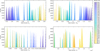 |
Fig. B.1 Distribution of our 100000 Monte Carlo simulation results for T126 for N2,CH4, H2 and Ar. As N2 increases, the dispersion of N2 and CH4 mole fraction decreases and their 1σ error varies from ±12 to 21 × 10−4. For Argon, the dispersion increases with its mole fraction and 1σ varies from ±1 to 3.5 × 10⁻⁷. For H2, 1σ ± 7 × 10⁻⁵. Each colour correspond to an altitude, from 1500 km (dark blue) to 950 km (yellow). |
The figure B.2 shows Ar40 mole fractions profile for flyby T5. No break of slope appears in our results.
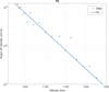 |
Fig. B.2 Ar40 mole fractions (in cm 3 vertical profiles for flyby T5. |
The figure B.3 shows 14N14N molecular density profiles, with the vertical line showing the altitude where the blue line doesn’t fit the data any more.
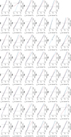 |
Fig. B.3 14N14N molecular density profiles for all flyby used in this study, fitted at high altitude (blue line), and low altitude (red line), with the vertical line showing the altitude where the blue line doesn’t fit the data any more. |
The figure B.4 shows N2 mole fractions profiles, with the delimited zones of transition for the altitude of the homopause graphically inferred.
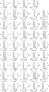 |
Fig. B.4 N2 mole fractions vertical profiles for all flyby used in this study. The grey area delimits the graphical transition zone of the homopause, and the red lines show the previous figure altitudes of break of slope in molecular density. |
All Tables
All Figures
|
Fig. 1 (Left) Percentage of differences between the retrieved N2 densities of flybys from Table A.1 using a temperature profile of 100 and 200 K. With a few exceptions, the difference is below 0.5%. Flybys T96, T97, T105, and T109 reach 30% of difference. (Right) N2 retrieved densities for all flybys for a constant T profile of 150 K. The colours depend on the flyby, and the density points are stacked and averaged. |
| In the text | |
|
Fig. 2 Vertical profiles of N2, CH4, Ar, and H2 mole fractions through time (filled squares). Note that all colour scales are linear except for H2. Mole fractions from flyby T64 (filled diamonds) come from Westlake et al. (2014).The solar longitude is indicated below the left graphs, with relevant longitudes corresponding to the years above. By convention the northern spring equinox corresponds to the solar longitude Ls = 0°. |
| In the text | |
|
Fig. 3 N2 molecular density for flybys T5, T27, T30, and T87. The top data points, fitted with plain lines, are the averaged molecular density of 14N 14N stacked over four data points. The bottom data points, fitted with dashed lines, are for 14N 15N molecular density. In blue and red are the fitted lines using equation 3 at high and low altitude, respectively, for 14N14N (plain) and 14N15N (dashed). The vertical lines are the altitudes below which 14N14N (plain) and 14N15N (dashed) data point cannot be fitted anymore by the blue curve. |
| In the text | |
|
Fig. 4 Upper and lower limits of the transition area between the homosphere and the heterosphere for each flyby from the mole fraction (grey) and the molecular density (red) of N2. The results from Waite et al. (2005) are in blue and those from Bell et al. (2011) are represented by the dashed grey line. |
| In the text | |
|
Fig. 5 N2 mole fraction as a function of latitude and time, at a constant altitude of 1300 km (left) and at a constant molecular density of 108 (right). |
| In the text | |
|
Fig. 6 Solar F10.7 cm radio flux over N2 mole fractions (left) and N2 density profiles (right). |
| In the text | |
|
Fig. B.1 Distribution of our 100000 Monte Carlo simulation results for T126 for N2,CH4, H2 and Ar. As N2 increases, the dispersion of N2 and CH4 mole fraction decreases and their 1σ error varies from ±12 to 21 × 10−4. For Argon, the dispersion increases with its mole fraction and 1σ varies from ±1 to 3.5 × 10⁻⁷. For H2, 1σ ± 7 × 10⁻⁵. Each colour correspond to an altitude, from 1500 km (dark blue) to 950 km (yellow). |
| In the text | |
|
Fig. B.2 Ar40 mole fractions (in cm 3 vertical profiles for flyby T5. |
| In the text | |
|
Fig. B.3 14N14N molecular density profiles for all flyby used in this study, fitted at high altitude (blue line), and low altitude (red line), with the vertical line showing the altitude where the blue line doesn’t fit the data any more. |
| In the text | |
|
Fig. B.4 N2 mole fractions vertical profiles for all flyby used in this study. The grey area delimits the graphical transition zone of the homopause, and the red lines show the previous figure altitudes of break of slope in molecular density. |
| In the text | |
Current usage metrics show cumulative count of Article Views (full-text article views including HTML views, PDF and ePub downloads, according to the available data) and Abstracts Views on Vision4Press platform.
Data correspond to usage on the plateform after 2015. The current usage metrics is available 48-96 hours after online publication and is updated daily on week days.
Initial download of the metrics may take a while.