| Issue |
A&A
Volume 708, April 2026
|
|
|---|---|---|
| Article Number | A92 | |
| Number of page(s) | 14 | |
| Section | Interstellar and circumstellar matter | |
| DOI | https://doi.org/10.1051/0004-6361/202556129 | |
| Published online | 30 March 2026 | |
One-dimensional and time-dependent modelling of complex organic molecules in protostars
1
Leiden Observatory, Leiden University,
PO Box 9513,
2300
RA
Leiden,
The Netherlands
2
Transdisciplinary Research Area (TRA) ‘Matter’/Argelander-Institut für Astronomie, University of Bonn,
Bonn,
Germany
3
Department of Physics and Astronomy, University College London,
Gower Street,
London,
UK
4
SURF,
Amsterdam,
The Netherlands
5
Leiden Institute of Chemistry, Leiden University,
2300
RA
Leiden,
The Netherlands
6
Institute for Molecules and Materials, Radboud University,
6525
AJ
Nijmegen,
The Netherlands
7
Institut de Recherche en Astrophysique et Planétologie, Université de Toulouse, CNRS, CNES,
9 av. du Colonel Roche,
31028
Toulouse Cedex 4,
France
8
Laboratoire d’astrophysique de Bordeaux, Univ. Bordeaux, CNRS, B18N, allée Geoffroy Saint-Hilaire,
33615
Pessac,
France
9
Korea Astronomy and Space Science Institute,
Daejeon
34055,
Republic of Korea
10
Korea University of Science and Technology,
217 Gajeong-ro, Yuseong-gu,
Daejeon
34113,
Republic of Korea
★ Corresponding author: This email address is being protected from spambots. You need JavaScript enabled to view it.
Received:
27
June
2025
Accepted:
22
December
2025
Abstract
Complex organic molecules (COMs), the building blocks of life, have been extensively detected under various physical conditions, from quiescent clouds to star-forming regions. They therefore serve as excellent tracers of the local physical and chemical properties of these environments. Proper models that are capable of grasping the formation and destruction of COMs are crucial to understanding observations. However, given that distinct COMs can be detected from different locations and at varying times, we improved UCLCHEM – a gas-grain chemical code – to a 1D, time-dependent model tailored to protostars. In this update, we examine two stages of a protostar, the prestellar and heating stages, incorporating a simple radiative mechanism for both the internal and external radiation fields of the cloud. This approach relies on the key assumption that the dust and gas temperatures are completely coupled. Ultimately, we implemented an updated version of our model to interpret observations obtained through both single-dish and interferometry under varying conditions, including a SgrB2(N1) hot core, massive Galactic clumps, and a hot core in Orion. We show that our model can reproduce these observations well. We highlight that some COMs are positioned at a higher temperature in the envelope, and others at a lower temperature, which could potentially leading to misinterpretations when using a single-point model. In the case of SgrB2(N1), the best model indicates that the cosmic-ray ionisation rate significantly exceeds the value typically used for the standard interstellar medium. Our model is as an efficient computational tool that will be particularly useful for gaining better insights into COM observations.
Key words: astrochemistry / stars: formation / ISM: abundances / dust, extinction / ISM: molecules
© The Authors 2026
 Open Access article, published by EDP Sciences, under the terms of the Creative Commons Attribution License (https://creativecommons.org/licenses/by/4.0), which permits unrestricted use, distribution, and reproduction in any medium, provided the original work is properly cited.
This article is published in open access under the Subscribe to Open model. This email address is being protected from spambots. You need JavaScript enabled to view it. to support open access publication.
1 Introduction
It is generally accepted that complex organic molecules (COMs, molecules with more than six atoms, see Herbst & van Dishoeck 2009) are the building blocks of life. A plethora of observations of COMs have been made towards hot cores associated with high-mass star-forming regions (see e.g. Cummins et al. 1986; Belloche et al. 2008; Requena-Torres et al. 2008; Belloche et al. 2019) and hot corinos associated with low-mass star-forming regions (see e.g. Ceccarelli et al. 2000; Jørgensen et al. 2012; Jiménez-Serra et al. 2016; Coutens et al. 2016; Martín-Doménech et al. 2017). Initially, COMs were believed to form within the ice mantles on dust particles and later convert to the gas phase when the dust grains are heated to 100–300 K (see, e.g., Garrod et al. 2008; Jiménez-Serra et al. 2016). However, COMs have also been detected in dark clouds and prestellar cores, where the temperature is rather low (see, e.g. Vastel et al. 2014; Agúndez et al. 2021; Ceccarelli et al. 2023). Various non-thermal processes have been proposed to desorb COMs, including photo-desorption, reactive desorption, cosmic-ray-induced desorption, and sputtering (see van Dishoeck 2014; Ceccarelli et al. 2023 for comprehensive reviews). An alternative gas-phase formation route for some COMs has also been proposed (Barone et al. 2015; Skouteris et al. 2017).
Chemical modelling is often used to understand observations of COMs and determine the chemical properties of the observed regions. Among others, the astrochemical open-source code UCLCHEM1 has been routinely used to interpret molecular observations (Holdship et al. 2017; Dutkowska et al. 2025; Vermariën et al., in prep.). This framework primarily uses a 0D and time-dependent model, incorporating the three-phase gas-grain chemical networks: the gas phase, surface, and bulk (every-thing below the surface). However, the existing UCLCHEM model restricts the capacity to identify the spatial distribution of the sources of COMs, which can introduce bias into the interpretation of the observations. In addition, interferometers provide remarkably high spatial resolution for observations of COMs, necessitating a model with higher spatial dimensionality.
Therefore, in this work, we improved the 1D treatment of radiation and visual extinction in the UCLCHEM framework, tailoring it to low- and high-mass protostars. Note that the UCLCHEM code could already simulate several gas cells (see, e.g. Viti & Williams 1999; Viti et al. 2004; Awad et al. 2010), albeit while maintaining the same values of the gas volume density and temperature for all cells, and disregarding the effect of the internal UV radiation field originated from the central source. Consequently, visual extinction and temperature are over-estimated. Additionally, photon-related phenomena may remain uncorrected; this happens when only the external radiation field is taken into account and the UV photons may not penetrate much towards the centre. However, incorporating an internal radiation field can facilitate the penetration of UV photons from the interior outwards. These effects influence chemical processes and can introduce biases. Our model physically follows the variations in the core’s envelope concerning physical properties such as gas densities, visual extinction, and temperature, potentially reducing the bias in predicting the abundance of COMs.
The structure of this paper is as follows. In Section 2, we describe the radial and time-dependent properties of the gas density, visual extinction, and dust temperature for our 1D model. The results of our qualitative comparisons with observations of various sources, including the SgrB2 (N1) hot core, Galactic massive clumps, and the Orion hot core, are given in Section 3. The limitations of our model are discussed in Section 4, and the conclusions of our work are presented in Section 5.
2 One-dimensional UCLCHEM modelling
This section describes our improvement of the distance- and time-dependent profiles for gas density, visual extinction, and temperature in our model.
We adhered to a conventional evolution of a protostar consisting of two distinct stages. The first is the collapsing (pre-stellar) phase, marked by material convergence due to gravitational instability, leading to a temporal rise in gas density and ultimately producing a density profile that follows a power-law decrease with radius. Consequently, various regions of the precursor cloud evolve at different rates; near the centre, because of the initially denser gas, this evolution proceeds more rapidly. The temperature is approximately constant through this stage because the radiation intensity from the surrounding medium is rapidly attenuated under such dense conditions. The next stage is the heating phase. During this stage, the physical phenomenon is the opposite. The formation of a protostar at the centre raises the temperature of the nearby gas and dust, and the gas density remains unvaried. Initially, the accretion process is the primary source of this heating, but as the protostar evolves, its luminosity takes precedence. Note that in proximity to the central luminous source, the dust particles are destroyed (no dust survives) if the temperature is higher than the sublimation temperature of the dust grain (e.g. Tthreshold ~ 1500 K for silicate grains; Hoang et al. 2015). When the temperature is below this threshold, there is a thin dust shell. This layer is irradiated by stellar radiation and plays an important role in heating the gas and dust in the outer zone. Figure 1 shows a sketch of the protostar scenario adopted in this work. Our assumption of the spherical protostellar core simplifies the source structure but we note that deviations from this model are supported by observations in the form of jets, outflows, and the disk. Such inclusions are beyond the scope of this work.
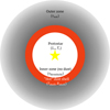 |
Fig. 1 Sketch of the protostellar core adopted in this model, including a central source characterised by the bolometric luminosity (L*) and the stellar temperature (T*). The inner zone is characterised by the sublimation threshold of dust grains (Tsub) and the threshold radius (rthreshold). The thin shell of hot dust is determined by the shell temperature (Tshell) and its radius (Rshell). The outer region is given by the outer radius (rout). |
2.1 Radial physical profiles: Gas densities and visual extinctions
We divided the radial profile into smaller S segments with a constant radial spacing. Each gas parcel was determined by the distance (r) to the centre. The gas volume density at a distance r in the cores was adopted in the Bonnor-Ebert sphere (Bonnor 1956) as
![Mathematical equation: $\[n_{\mathrm{gas}}(r)= \begin{cases}n_0 & \text { for } r \leq r_0, \\ n_0\left(\frac{r}{r_0}\right)^{-\alpha} & \text { for } r>r_0,\end{cases}\]$](/articles/aa/full_html/2026/04/aa56129-25/aa56129-25-eq1.png) (1)
(1)
where n0 is the maximum density in the centre and is a parameter of our model, along with α and r0.
In a given gas cell, the gas column densities from the centre to that cell (![Mathematical equation: $\[N_{\text {gas}}^{\text {centre2cell}}\]$](/articles/aa/full_html/2026/04/aa56129-25/aa56129-25-eq2.png) ) and from the edge of the envelope to that cell (
) and from the edge of the envelope to that cell (![Mathematical equation: $\[N_{\text {gas}}^{\text {edge2cell}}\]$](/articles/aa/full_html/2026/04/aa56129-25/aa56129-25-eq3.png) ) are
) are
![Mathematical equation: $\[\begin{aligned}N_{\mathrm{gas}}^{\text {centre2cell }}(r) & = \begin{cases}n_0 r & \text { for } r \leq r_0, \\n_0 r_0+\frac{n_0 r_0}{\alpha-1}\left[1-\left(\frac{r}{r_0}\right)^{-\alpha+1}\right] & \text { for } r>r_0,\end{cases} \\N_{\mathrm{gas}}^{\text {edge2cell }}(r) & = \begin{cases}n_0 r_0\left(\frac{\alpha}{\alpha-1}-\frac{r}{r_0}\right) & \text { for } r<r_0, \\\frac{n_0 r_0}{\alpha-1}\left(\frac{r}{r_0}\right)^{1-\alpha} & \text { for } r>r_0,\end{cases}\end{aligned}\]$](/articles/aa/full_html/2026/04/aa56129-25/aa56129-25-eq4.png) (2)
(2)
The corresponding visual extinctions are computed as
![Mathematical equation: $\[\begin{aligned}A_{\mathrm{V}}^{\text {centre2cell }}(r) & =N_{\text {gas}}^{\text {centre2cell}} / 1.61 \times 10^{21} ~\mathrm{mag}, \\A_{\mathrm{V}}^{\text {edge2cell}}(r) & =N_{\text {gas }}^{\text {edge2cell}} / 1.61 \times 10^{21} ~\mathrm{mag}.\end{aligned}\]$](/articles/aa/full_html/2026/04/aa56129-25/aa56129-25-eq5.png) (3)
(3)
2.2 Radial physical profiles: radiation field and temperatures
To consistently model the 1D effects of radiation, we first calculated the radiation from the protostars as well as the radiation from the thin dust shell and then derived the temperature.
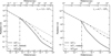 |
Fig. 2 Variations in stellar and dust shell radiations with respect to radial distance for low-mass (left panel) and high-mass (right panel) protostellar cores. For r < rthreshold (marked by the vertical dashed-dotted line), the stellar radiation decreases as U(T*, nodust) ~r−2. For r > rthreshold, this stellar radiation (U(T*)) is quickly reduced because of dust attenuation. The radiation in the outer region is mainly dominated by the emission from the dust shell (U(Tshell)). |
2.2.1 Stellar radiation
The dimensionless energy density of the radiation at a distance r from the centre is calculated as
![Mathematical equation: $\[U\left(T_*\right)=\frac{\int_{0.091 ~\mu \mathrm{m}}^{20 ~\mu \mathrm{m}} u_\lambda\left(T_*\right) e^{-\tau_\lambda} d \lambda}{u_{\mathrm{ISRF}}}\]$](/articles/aa/full_html/2026/04/aa56129-25/aa56129-25-eq6.png) (4)
(4)
where uλ(T*) = Lλ(T*)/(4πr2c) is the spectral energy density for no dust obscured, uISRF = 8.64 × 10⁻¹³ erg cm−3 is the energy density of the interstellar radiation field, and τ is the optical depth. We assumed that the centre emits as a black body, which yielded
![Mathematical equation: $\[u_\lambda(T_*)=\frac{4 \pi R_*^2 \pi B_\lambda(T_*)}{4 \pi r^2 c}.\]$](/articles/aa/full_html/2026/04/aa56129-25/aa56129-25-eq7.png) (5)
(5)
The optical depth is determined by the extinction curve as
![Mathematical equation: $\[\tau_\lambda=\left(A_\lambda / A_{\mathrm{V}}\right) \times A_{\mathrm{V}}^{\text {centre2cell }} / 1.086\]$](/articles/aa/full_html/2026/04/aa56129-25/aa56129-25-eq8.png) (6)
(6)
with the extinction curve (Aλ/AV) adopted from Cardelli et al. (1989).
The dust survival distance, rthreshold, is intrinsically dependent on the threshold temperature (Tthreshold) of the grain material (above which the grains are destroyed by sublimation) and is approximated, as in Hoang (2021), as2
![Mathematical equation: $\[r_{\text {threshold }} \simeq 155.3\left(\frac{L_{\text {bol }}}{10^6 L_{\odot}}\right)^{0.5}\left(\frac{T_{\text {threshold }}}{1500 \mathrm{~K}}\right)^{-5.6 / 2} ~\mathrm{au}\]$](/articles/aa/full_html/2026/04/aa56129-25/aa56129-25-eq9.png) (7)
(7)
with Tthreshold = 1500 K as in Hoang et al. (2015). We observe that stellar radiation decreases as r−2 for r < rthreshold, but is more greatly attenuated due to the additional optical depth for r ≥ rthreshold. In this work, we focused solely on the positions where r ≥ rthreshold (that is, where dust can survive).
2.2.2 Radiation from the dust shell
The ‘hot’ dust shell absorbs the stellar radiation from the source and re-emits as thermal emission farther out in the envelope. At a distance r > rthreshold in the outer region, the dimensionless radiation energy density attributed by this shell is
![Mathematical equation: $\[\begin{aligned}U\left(T_{\text {shell }}\right) & =\frac{\int_{0.091 ~\mu \mathrm{m}}^{20 ~\mu \mathrm{m}} L_\lambda\left(T_{\text {shell }}\right) e^{-\tau_\lambda} d \lambda}{4 \pi r^2 c u_{\text {ISRF }}} \\& =\frac{\int_{0.091 ~\mu \mathrm{m}}^{20 ~\mu \mathrm{m}} 4 \pi R_{\text {shell }}^2 \pi B_\lambda\left(T_{\text {shell }}\right) e^{-\tau_\lambda} d \lambda}{4 \pi r^2 c u_{\text {ISRF }}}\end{aligned}\]$](/articles/aa/full_html/2026/04/aa56129-25/aa56129-25-eq10.png) (8)
(8)
where Tshell is calculated from U(T*)(r = rthreshold) with an assumption that the hot shell is thin enough (dshell ≪ 1) to prevent any radiative processes from occurring within it, resulting in the constant temperature of the shell (Tshell(Rshell) = Tshell(Rshell + dshell)).
It is worth noting that the stellar radiation is responsible for the inner zone, while the dust shell at longer wavelengths is primarily responsible for heating in the outer regions (i.e. U(T*) ≪ U(Tshell) when r ≫ rthreshold). For example, a high-mass protostar with T* = 4.5 × 10⁴ K has a maximum emitted wavelength of approximately 65 nm, which is in the far ultraviolet (UV) range. The ultraviolet photons from the star are absorbed quickly after the dust shell. For lower-mass protostars, the peak of the radiation energy spectrum is shifted to a longer wavelength, and the photons can penetrate more deeply into the outer region, but the dust shell is still dominant for r ≫ 1. These features are shown in Figure 2 with the mean wavelengths for these two radiation fields decomposed in Figure A.1.
2.2.3 Temperature profile
If the dust is in equilibrium, which is a reasonable assumption in the case of large dust grains, the dust temperature is related to the radiation intensity as shown in Draine (2011) as
![Mathematical equation: $\[\begin{aligned}T_{\mathrm{d}}^{\mathrm{sil}}(r) & =16.4 \mathrm{~K} \times\left[U\left(T_*\right)+U\left(T_{\text {shell }}\right)\right]^{1 / 6} \qquad\text {silicate}\\T_{\mathrm{d}}^{\mathrm{car}}(r) & =19.5 \mathrm{~K} \times\left[U\left(T_*\right)+U\left(T_{\text {shell }}\right)\right]^{1 / 5.6} \quad~\text {carbonaceous}\end{aligned}\]$](/articles/aa/full_html/2026/04/aa56129-25/aa56129-25-eq11.png) (9)
(9)
where U(T*) and U(Tshell) are the functions of distance and calculated from Eqs. (4) and (8). The dust temperature is taken as the average as ![Mathematical equation: $\[T_{\mathrm{d}}(r)=\left[0.625 \times\left(T_{\mathrm{d}}^{\mathrm{sil}}\right)^{4}+0.375 \times\left(T_{\mathrm{d}}^{\mathrm{car}}\right)^{4}\right]^{1 / 4}\]$](/articles/aa/full_html/2026/04/aa56129-25/aa56129-25-eq12.png) with silicate and carbonaceous referring to the dust composition. Figure 3 shows the radial profiles for both the gas density (solid line on the left y-axis) and the dust temperature (dashed line on the right y-axis) corresponding to four different protostars with a luminosity of L* ~ 103−106 L⊙. The gas density remains uniform up to r0 and decreases beyond this point. The dust temperature sharply reduces towards the surface as a result of the attenuation of the radiation field. These values of gas density and dust temperature at each radius are specified for the final values (when t → ∞) in the time-dependent evolution at this position. As a benchmark, we compared the dust temperature profiles in our model with those in Sabatini et al. (2021) and Nomura & Millar (2004) for the same central luminosity sources and found consistent temperature profiles. The temperature values at the very far edges of the envelope are for comparison with the literature. In practice, we stopped at T ~ 10-20 K as shown in Table 2.
with silicate and carbonaceous referring to the dust composition. Figure 3 shows the radial profiles for both the gas density (solid line on the left y-axis) and the dust temperature (dashed line on the right y-axis) corresponding to four different protostars with a luminosity of L* ~ 103−106 L⊙. The gas density remains uniform up to r0 and decreases beyond this point. The dust temperature sharply reduces towards the surface as a result of the attenuation of the radiation field. These values of gas density and dust temperature at each radius are specified for the final values (when t → ∞) in the time-dependent evolution at this position. As a benchmark, we compared the dust temperature profiles in our model with those in Sabatini et al. (2021) and Nomura & Millar (2004) for the same central luminosity sources and found consistent temperature profiles. The temperature values at the very far edges of the envelope are for comparison with the literature. In practice, we stopped at T ~ 10-20 K as shown in Table 2.
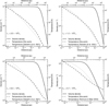 |
Fig. 3 Examples of radial profiles of the gas density (solid line, left y-axis) and dust temperature (dashed line, right y-axis) in protostars of different L* embedded in a molecular core for r ≥ rthreshold. In each panel, our temperature profile is compared to the profiles found in the literature. For the profiles from Sabatini et al. (2021), we used n0 = 107 cm−3 and r0 = 0.15 pc, the same as the authors. For the profile from Nomura & Millar (2004), we used n0 = 1.5 × 106 cm−3 and r0 = 0.05 pc. |
2.3 Time-dependent physical profiles: Pre-stellar stage
For a given gas parcel with boundary location ri, we modelled the change in physical properties over time as follows. In the pre-stellar collapse phase, the gas volume density increases from an initial n0 (t = 0, r) to ngas (t → ∞, r) described in Eq. (1) as
![Mathematical equation: $\[\begin{aligned}\frac{d n\left(t, r_i\right)}{d t}=~ & b_c\left(\frac{n\left(t, r_i\right)^4}{n\left(t=0, r_i\right)}\right)^{1 / 3} \\& \times\left[24 \pi G m_{\mathrm{H}} n\left(t=0, r_i\right)\left(\left(\frac{n\left(t, r_i\right)}{n\left(t=0, r_i\right)}\right)^{1 / 2}-1\right)\right]^{1 / 2}\end{aligned}\]$](/articles/aa/full_html/2026/04/aa56129-25/aa56129-25-eq13.png) (10)
(10)
with bc = 1 the freefall factor, G the gravitational constant, and mH representing the mass of hydrogen nuclei. The collapse continues until the gas reaches the final density ngas aimed at a specific gas parcel. To mimic the fact that the initial gas volume density is denser towards the centre, we calculated the term n(t = 0, r) from Eq. (1) with n0 = 2.18 × 104 cm−3 and r0 = 1.4 × 10⁴ au (see Eqs. (7) and (8) in Priestley et al. 2018).
For each gas parcel, the column density is evaluated at every time step using the expression
![Mathematical equation: $\[\Delta N_{\mathrm{gas}}(r_i, t)=\frac{r_{\mathrm{out}}}{\mathrm{~S}} n_{\mathrm{gas}}(r_i, t).\]$](/articles/aa/full_html/2026/04/aa56129-25/aa56129-25-eq14.png) (11)
(11)
The cumulative column density extending from the cloud’s edge to that parcel is then given by
![Mathematical equation: $\[N_{\mathrm{gas}}^{\mathrm{edge} 2 \mathrm{cell}}(r, t)=\sum_{r_i=r_{\mathrm{out}}}^r \Delta N_{\mathrm{gas}}(r_i, t)\]$](/articles/aa/full_html/2026/04/aa56129-25/aa56129-25-eq15.png) (12)
(12)
which allows the visual extinction (![Mathematical equation: $\[A_{\mathrm{V}}^{\text {edge2cell}}(r, t)\]$](/articles/aa/full_html/2026/04/aa56129-25/aa56129-25-eq16.png) ) to be calculated at each time step as well, using Eq. (3).
) to be calculated at each time step as well, using Eq. (3).
It is important to highlight that within our approximation, when t approaches infinity, we have limt→∞ ngas(r, t) → ngas(r), as defined in Eq. (1). Similarly, ![Mathematical equation: $\[{\lim}_{t \rightarrow \infty} N_{\text {gas}}(r, t) \rightarrow N_{\text {gas}}^{\text {edge2cell}}(r)\]$](/articles/aa/full_html/2026/04/aa56129-25/aa56129-25-eq17.png) , as defined in Eq. (2), and limt→∞ AV(r, t) → AV(r), as defined in Eq. (3).
, as defined in Eq. (2), and limt→∞ AV(r, t) → AV(r), as defined in Eq. (3).
2.4 Time-dependent physical profiles: Heating stage
We turned on the central luminosity source (the protostar) after the pre-stellar stage. The gas and dust were heated by different mechanisms at different times, such as accretion, photospheric luminosity from gravitational contraction, and deuterium burning in the central star. As we did not model the evolution of the central luminosity, we assumed that at a point r, the evolution of the gas and dust temperature from Td(t = 0, r) to Td(t → ∞, r) (described in Eq. (9)) is characterised by an empirical relation as in Awad et al. (2010) as
![Mathematical equation: $\[T_{\mathrm{d}}(t, r)=T_{\mathrm{d}, 0}+A t^B\left(\frac{r}{r_{\text {out }}}\right)^{-\beta} \quad\mathrm{K}\]$](/articles/aa/full_html/2026/04/aa56129-25/aa56129-25-eq18.png) (13)
(13)
with the constants A and B defining the curvature of Td versus time, and Td,0 = 10 K, the temperature of the ambient gas. Figure 3 shows that Td ~ r−0.5, and we then adopted β = 0.5. The values of A and B were derived from combinations of
Td (t = 0, r) = 10 K
and Td(r) in Eq. (9) with
Td(r) = 100 K after 105 yr for 1 × M⊙ star (Awad et al. 2010) or
Td(r) = 100 K after 105 yr for 5 × M⊙ star or
Td(r) = 300 K after 2 × 10⁵ yr for 10 × M⊙ star or
Td(r) = 200 K after 1.1 × 10⁵ yr for 15 × M⊙ star (Viti & Williams 1999; Viti et al. 2004) or
Td(r) = 200 K after 7 × 10⁴ yr for 25 × M⊙ star (Viti & Williams 1999) or
Td(r) = 200 K after 2.8 × 10⁴ yr for 60 × M⊙ star (Viti & Williams 1999).
During this stage, the additional attenuation from the central source is characterised by the visual extinction from the centre to the parcel as ![Mathematical equation: $\[A_{\mathrm{V}}^{\text {centre2cell}}(r, t) \equiv A_{\mathrm{V}}^{\text {centre2cell}}(r)\]$](/articles/aa/full_html/2026/04/aa56129-25/aa56129-25-eq19.png) as computed in Eq. (3), due to the constant gas volume density.
as computed in Eq. (3), due to the constant gas volume density.
2.5 UV radiation fields
In the heating stage, we added the UV radiation field from the central source (internal UV field), in addition to the external ![Mathematical equation: $\[G_{0}^{\text {ext}}\]$](/articles/aa/full_html/2026/04/aa56129-25/aa56129-25-eq20.png) , which is a parameter in our model. This internal field solely depends on the luminosity in the UV bands (LUV) of the source and is defined at the dust shell as
, which is a parameter in our model. This internal field solely depends on the luminosity in the UV bands (LUV) of the source and is defined at the dust shell as
![Mathematical equation: $\[G_0^{\mathrm{int}}=\frac{L_{\mathrm{UV}, *}}{4 \pi c r_{\text {threshold}}^2 5.29 \times 10^{-14} \mathrm{erg} \mathrm{~cm}^{-3}}\]$](/articles/aa/full_html/2026/04/aa56129-25/aa56129-25-eq21.png) (14)
(14)
where LUV,* is the integration of the luminosity of the central source, approximately a black body from 0.6 to 13.6 eV, which yields LUV,* = 0.4–0.5 × L*. For a given position at a given time, this internal UV field is attenuated as ![Mathematical equation: $\[G_{0}^{\text {int}} e^{-A_{\mathrm{V}}^{\text {centre2cell}}}\]$](/articles/aa/full_html/2026/04/aa56129-25/aa56129-25-eq22.png) .
.
2.6 Chemical network
In the version described in this study, the reaction network comprises 356 species and 8766 gas-phase reactions sourced from the latest UMIST22 database (Millar et al. 2024). The grain reactions are taken from Holdship et al. (2017) and Quénard et al. (2018). The species in the chemical network are denoted as, for example, H2O (gas-phase water), #H2O (surface water), @H2O (bulk water), and $H2O (ice water), with ice being the sum of surface and bulk.
Our model contains both thermal and non-thermal mechanisms to desorb the species from the surface into the gas phase. The latter processes include UV radiation, molecular hydrogen formation, direct cosmic rays, cosmic-ray-induced UV, and chemical desorption. It also includes the competition of Langmuir-Hinshelwood reactions by diffusion and desorption as described by Chang et al. (2007). We refer the reader to Quénard et al. (2018) and Dutkowska et al. (2025) for a complete description of the chemical network used.
UCLCHEM starts with gas species in atomic or ionic forms (see Table 1 for the total abundances related to hydrogen of elementary species) without molecules. For hydrogen, half is atomic and the other half is molecular. During the collapse phase, chemical reactions occur, leading to the formation of molecules within the gas phase and ice mantles on dust particles. The end abundances of this stage serve as the initial conditions for the subsequent heating stage.
Total initial elemental abundances with respect to the total number of hydrogen nuclei (H).
Range of radial distance from the centre for low-mass and high-mass protostars.
3 Results and applications
3.1 Distance- and time-dependent physical properties of a molecular core
Figure 4 shows an example of the time-dependent physical profiles for different gas parcels estimated from our model. The top panel shows that parcels closer to the centre, in the prestellar phase, experience a faster evolution of their gas volume density because their initial n(t = 0) is higher. When they reach the final value assigned to their positions (estimated by Eq. (1)), they remain constant.
The middle panel shows the corresponding profiles of the visual extinction from the edge inwards. Similarly to the gas density profile, the gas parcel deeper inside the core quickly becomes obscured as the visual extinction increases to at least two orders of magnitude higher than the edge.
The bottom panel illustrates the time-dependent profile of the temperature. During the pre-stellar stage, this profile remains constant at 10 K. During the heating stage, as the central source heats up, the gas temperature rises to its final value at the specified location depicted in Figure 3. Due to attenuation, the gas parcels closer to the centre experience a more rapid temperature increase compared to those situated farther out in the cloud.
Key physical parameters for the modelling along the west and south directions of the SgrB2(N1) hot core.
3.2 Distance- and time-dependent chemical properties of a molecular core
Figure 5 shows an example of the variation of the gas-phase CH3OH over time for 100 gas parcels from the centre for two particular cases of L⊙ (left panel) and 105 L⊙ (right panel). Two distinct features are seen: the abrupt increase in the abundance in proximity to the central source is due to the thermal sublimation. In the envelope, where the temperature is below 100 K, the abundance of CH3OH is rather low due to the majority of molecules being frozen on the grains. Non-thermal desorption processes desorb a limited amount of CH3OH molecule. For gas parcels with the highest temperatures, the abundances of CH3OH and other complex molecules are seen to rapidly decrease at late times; our chemical analysis shows that the reactions of neutral ions drive this destruction. For example, the most destructive reaction to destroy CH3OH at 5 × 10⁵ yr is H3O+ + CH3OH → CH3OH2+ + H2O with a rate of −4.17 × 10⁻¹⁹ cm−3 s−1.
Figure 6 illustrates how the gas-phase abundance of selected COMs changes with the radial distance for low-mass and high-mass protostars. For methanol, Figure 5 shows that the abundance reaches its peak and remains uniform near the core, subsequently decreasing as it extends towards the envelope. A more luminous central source results in a larger region where the abundance is constant. The input parameters are listed in Table 2.
3.3 Application: COM abundances in the SgrB2 (N1) hot core
In this section, we compare the predictions of our model with the spatial distribution of abundances of some COMs reported by Busch et al. (2022) within the ReMoCA (Re-exploring Molecular Complexity with ALMA) survey (Belloche et al. 2019). This survey used ALMA (Atacama Large Millimeter Array) to observe towards the hot core N1 in the giant molecular cloud Sagittarius B2-North (hereafter SgrB2(N1)). The observations are made with different setups, covering an angular resolution from 0.75″ in setup 1 to 0.3″ in setup 5 (we refer to Table 2 in Belloche et al. 2019 for more details). The abundances are taken in two directions: west and south from the central hot core.
We modelled the radial abundances of some oxygen-bearing COMs, including CH3OH, CH3OCH3, C2H5OH, NH2CHO, and CH3CHO with the main input parameters described in Table 3. The luminosity and the mass of the central source were fixed, while we adjusted the parameter r0 because it regulates the gas volume density profile and thus regulates the radiative process. The best values of r0 are based on a comparison of the radial profile of X(CH3OH) from the model and observations. Finally, we varied the cosmic rate ionisation rate from the standard value in the interstellar medium (ISM; ζISM = 1.3 × 10⁻¹⁷ s−1) with a scale factor (ζscale = [1, 100]); then the cosmic-ray ionisation rate at each location and time step in our model is ζ/ζISM × ζscale where the cosmic-ray attenuation towards the centre is considered following O’Donoghue et al. (2022) as ![Mathematical equation: $\[\log _{10} \zeta={\sum}_{k=0}^{9} c_{k} ~\log _{10}^{k}(N_{\mathrm{gas}}^{\text {edge2cell}})\]$](/articles/aa/full_html/2026/04/aa56129-25/aa56129-25-eq23.png) with the coefficient ck given in their Table A1 (model ℒ). The external UV radiation field is adopted as 103 times higher than the typical interstellar radiation field with G0,ISM = 1 (see, e.g., Goicoechea et al. 2004).
with the coefficient ck given in their Table A1 (model ℒ). The external UV radiation field is adopted as 103 times higher than the typical interstellar radiation field with G0,ISM = 1 (see, e.g., Goicoechea et al. 2004).
For each COM, we compared the predicted profiles with observations over time to determine the best fits of the model and time, using the minimum of χ2 as
![Mathematical equation: $\[\chi^2=\sum_{i=1}^N\left[\frac{\ln (X_{\text {model}})-\ln (X_{\text {obs}, \mathrm{i}})}{\ln (X_{\text {obs}, \mathrm{i}})}\right]^2.\]$](/articles/aa/full_html/2026/04/aa56129-25/aa56129-25-eq24.png) (15)
(15)
The summation is taken for all data points N, and the predicted Xmodel is interpolated at the corresponding distance as in observations. The left panel of Figure 7 shows the comparison of the radial profile of the COMs predicted from our model with observations in the west direction towards the central hot core SgrB2(N1). We note that our model can reproduce these profiles reasonably well for a higher cosmic-ray ionisation rate with ζscale ≃ 30, corresponding to the value of ζ(0.2 pc) ≃ 60 × ζISM (see Figure B.1 for the radial profile of ζ). Nonetheless, our model cannot explain the observed profile of C2H5OH (Xobs(C2H5OH) ≃ 10−7). The explicit explanation is beyond the scope of this work and requires more extensive work. However, we discuss this issue in Section 3.4.
Similarly, the right panel of Figure 7 shows the comparison for the south direction. Along this direction, CH3OH begins to decrease further from the centre (> 0.1 pc) compared to its decline along the west direction. As in the previous case, models with higher cosmic-ray ionisation rate are required (ζ(0.2 pc) ≃ 50 × ζISM with the best ζscale = 20, see Figure B.1) to reproduce all detections, but the prediction for the abundance of C2H5OH is again too low compared to observations. The cosmic ray ionisation rates derived from our models for the hot core SgrB2(N1) are consistent with those of Bonfand et al. (2019), in which the authors show that ζ ≥ 50 × ζISM using the observations of COMs in the nearby hot cores SgrB2(N2-N5).
It is important to note that the abundance decreases more rapidly to the west from the centre compared to the south. Furthermore, the value of rflat is higher in the southern direction, suggesting a higher gas density in the south than in the west, consistent with Figure 8 in Busch et al. (2022) and with the lower value of ζ predicted by our model in the south due to attenuation.
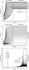 |
Fig. 4 Examples of the profiles of the gas density (top), visual extinction from the surface (middle) and temperature (bottom). The negative time is for the pre-stellar phase, and a time of zero is when the protostar is formed. For visualisation purposes, 50 of the 100 gas parcels in the sampling are shown. The values of ngas(r) estimated by Eq. (1) and the Td(r) estimated by Eq. (9) are the final values of ngas(t) in Eq. (10) and Td(t) in Eq. (13) at a given location r. These profiles have L* = 105 L⊙, nin = 107 cm−3, rflat=0.05 pc and a = 0.5 μm. |
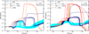 |
Fig. 5 Example of the variation in CH3OH with time for L* = 100 L⊙ (left) and L* = 105 L⊙ (right). Lines are for the 100 parcels (full grid) from the center, color-coded by the temperature at t = 106 yr. The abundance of CH3OH decreases sharply at late times because of the reaction with neutral and ion species. For instance, at t = 5 × 10⁵ yr, the most important destruction reactions are H3O+ + CH3OH → CH3OH2+ + H2O and H3+ + CH3OH → CH3+ + H2O + H2. |
3.4 Application: COM abundances in massive protostars
In this section, we assess our model’s predictions against APEX (Atacama Pathfinder EXperiment) observations of three massive protostars in our Galaxy: G328.25, G335.58, and G335.78 reported in Bouscasse et al. (2024). The observations were made using different receivers of the APEX, whose beam size ranged from 18″ to 36″, and the abundances relative to the gas column density were scaled to the size of the observed emission area (cf. Section 5.6 in Bouscasse et al. 2024). The luminosities of these sources are approximately the same as 104 L⊙ as noted in Table 1 in Bouscasse et al. (2024), the differences in the observed COMs are not influenced by the radiative characteristics of these sources, which presents a perfect scenario for exploring other effects, such as the physical conditions of the sources. In this work, we examined some specific oxygen-bearing COMs, including CH3OH, NH2CHO, CH3OCH3, and C2H5OH, for which Bouscasse et al. (2024) demonstrated that the single-point model in Garrod et al. (2022) overestimates the abundances of these COMs (see their Figure 13). The authors suggested that the overestimation may arise due to the fact that the sources are in a stage where non-thermal sublimation predominantly determines abundances, whereas the thermal sublimation area is compact.
Figure 8 shows the lower and upper limits of our models (the shaded area in the largest panel) that cover the observed abundance of each species at a given time (the limits, both lower and upper, are determined by the distances r1 and r2 of the model where the abundances X(r1) < X(obs) < X(r2)). This plot is for particular time values of 7 × 10⁴ yr and a grain size of 0.5 μm (the effect of the grain size is shown in Figure C.1). The height of these areas is due to the model’s grid at that given time. From these best models, we determined the gas parcels from which the COMs are detected, and the temperature ranges highlighted by the colour lines in the corresponding upper and lower panels. Our temperature range is found to be roughly consistent with the excitation temperatures for these COMs in Bouscasse et al. (2024) (see their Figure 11).
We compared our best models with the single-point (0D) model of the original UCLCHEM with a standard UV field (G0 = 1) and the one presented in Garrod et al. (2022)3. The 0D models tend to overestimate the abundance of the considered COMs, except for X(NH2CHO), whereas our 1D model matches more closely with the observational data. This discrepancy arises because these COMs originate from different regions, necessitating the physical structure to be considered. For example, for temperatures exceeding 100 K (thermal desorption dominates), our models predict abundance (X(CH3OH), X(CH3OCH3) and X(C2H5OH)) similar to those of the Garrod et al. 2022 model. It is important to mention that, unlike Garrod et al. (2022), our model does not incorporate non-diffusive chemistry.
Interestingly, the 0D model can predict a higher X(C2H5OH), which can better explain the observations in the SgrB2(N1) hot core mentioned in Section 3.3. Therefore, we performed a series of tests with the 0D model to understand why our 1D model could not predict the observed high abundance. We found that COMs become significantly less abundant when using higher values of G0 (see Figure C.2). In our 1D model, the high abundance of C2H5OH near the centre is affected by the internal UV field generated by the central source rather than by the external UV field. Therefore, the low abundance of C2H5OH may be an indication either that the UV field profile in our 1D model is not correct or that we lack key chemical reactions for this species, such as non-diffusive reactions. If the former is true, it remains unclear why only C2H5OH is too sensitive.
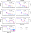 |
Fig. 6 Abundance of various COMs as a function of distance based on different source luminosities at different ages. While the chosen age is arbitrary, it is consistent with the fact that a more massive protostar evolves faster than the less massive one. Typically, the abundance remains unchanged near the centre and decreases farther out. In the case of a more massive protostellar core, the abundance extends over a larger volume. |
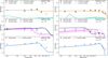 |
Fig. 7 Radial profiles of some COMs as a function of radial distance moving westwards (left panel) and southwards (right panel) from the SgrB2(N1) hot core with G0 = 103. The symbols represent observational data. The prominent solid lines illustrate the best models (the lighter lines denote models corresponding to the ages within ±1σ around the age determined by the best χ2). Our model can nicely reproduce the radial profiles of CH3OH, CH3OCH3, NH2CHO and CH3CHO but fails to explain the C2H5OH profile. To better match observations for all COMs, the cosmic ray ionisation rate is required to be higher than the typical value of the ISM. For the westwards, ζscale = 30 corresponds to ζ(0.2 pc) ≃ 60 × ζISRF, and ζscale = 20 corresponds to ζ(0.2 pc) ≃ 50 × ζISRF for the southwards. The best-fit period correspond to (3–7) × 104 yr. |
3.5 Application: COM abundances in the Orion hot core
In this section, we compare our model with ALMA observations towards the methyl formate (MF) peak, the ethylene glycol (EG) peak, and the ethanol (ET) peak in the nearby hot core in the Orion BN/KL region as reported in Tercero et al. (2018) at a resolution of ~1.5″. In this case, the central source luminosity is about 105 L⊙. Figure 9 presents a comparison of the specific abundances of CH3OH, CH3OCH3, HCOOH, and C2H5OH as predicted by our model (represented by shaded areas in the largest subfigure) at a given specific cloud age and those observed (indicated by coloured symbols; taken from Table 2 in Tercero et al. 2018) in Orion BN/KL. In general, our model is effective in explaining the observed abundances and shows that the emitting regions of these COMs change with the cloud’s age (colour lines in the figures on the top and bottom). The best coverage shows that CH3OH, CH3OCH3, and C2H5OH originate at higher temperatures compared to HCOOH, and our model cannot reproduce X(C2H5OH ~ 3.5 × 10⁻⁸) at the Orion ET peak. The potential explanation might be an excessively strong UV field or the absence of chemical reactions involving C2H5OH as discussed in Section 3.4.
4 Limitations
There are three main sources of uncertainty in our model: the decoupling in the temperature of the dust and the gas, the beam average and the structure of the envelope. We discuss each of these caveats in the following.
First, our model does not incorporate the heating and cooling processes, which might affect the temperature distributions of gas and dust and subsequently result in different COM abundances as discussed in this study. The gas-dust coupling, which is expected to hold during the heating stage, may in fact not hold at lower densities (e.g. Ivlev et al. 2019 shows that Tdust ≃ Tgas for nH ≥ 106 cm−3); therefore, the impact of the heating and cooling processes will primarily be significant in the collapse phase. To explicitly understand how these effects could impact predicted abundances of COMs, our upcoming work will incorporate the decoupling of the temperatures of the dust and gas.
Second, the predicted quantities of COMs from our 1D model do not incorporate the beam average, which introduces bias when compared to observations, particularly those from single-dish observations. This factor necessitates employing a model of a higher dimension than our current 1D approach, since it is essential to accurately compute the COMs density across all sight lines within a spatial region before convolving into the intended beam size. Note that along each line of sight, the physical profiles of density and temperature vary differently from the radial profile adopted from the 1D model.
Third, the physical characteristics of the protostellar cores do not account for the presence of clumpy structures or outflows or variations in luminosity. We expect the temperature profile to be more extended in the clumpy envelope, since the radiative transfer processes differently from the smoothed continuous envelope in this work. We notice that our model can be further improved by adapting the time-dependent luminosity of the protostellar cores (e.g., see Figure 3a in Choudhury et al. 2015).
5 Conclusions
In this study, we updated the 0D-UCLCHEM chemical modelling of protostars to a simple and computationally efficient 1D, time-dependent model. We then compared the predictions of our novel model with existing observations of a range of astronomical targets: a SgrB2(N1) hot core (Figure 7), infrared-quiet galactic massive clumps (G328.25, G335.58, G335.78) (Figure 8), and the hot core in Orion BN/KL (Figure 9). We summarise our findings below:
We considered the formation of a protostar as happening in two phases: collapse and heating. Initially, during the collapse stage, the gas volume density increases over time and the temperature remains fixed. In the subsequent heating phase, a luminous source at the core is activated (controlled by the bolometric luminosity), leading to a temperature increase without altering the density. Initially, the gas is denser near the core, and the dust temperature is estimated using a basic radiative transfer setup, assuming an equilibrium between the radiation field and temperature.
Comparison with the SgrB2(N1) hot core: We used the ALMA observations within the ReMoCA survey, reported in Busch et al. (2022) for CH3OH, CH3OCH3, C2H5OH, NH2CHO, and CH3CHO. The radial profile of COMs along two distinct directions (westwards and southwards from the centre) illustrates the drop in abundance away from the central source. Our models can successfully reproduce these observational features but require a high cosmic-ray ionisation rate (e.g. at least 50–60 times higher than the accepted standard value of the ISM at 0.2 pc from the centre).
Comparison with Galactic massive clumps (G328.25, G335.58, and G335.78): The observations of CH3OH, NH2CHO, CH3OCH3, and C2H5OH towards massive infrared-quiet clumps (objects with bolometric luminosities less than 2 × 10⁴L⊙), reported by Bouscasse et al. (2024), were conducted with the single-dish APEX telescope. The models that best reproduce these observations suggest temperature ranges that are broadly in line with the derivations from the observations. The need for an accurate treatment of the radiation and extinction in one dimension of the source structure is underscored by the way distance affects the data interpretations, as utilising a single-point model for a hot core and/or hot corino could lead to an overestimation of COMs if they do not originate sufficiently near the central luminosity.
Comparison with ALMA observations towards Orion BN/KL: We considered only CH3OH, CH3OCH3, HCOOH, and C2H5OH towards three well-known locations in the Orion BN/KL, i.e. the MF, EG, and ET peaks as reported in Tercero et al. (2018). Our model can nicely reproduce these observations, except for C2H5OH at the ET peak, showing that the HCOOH-emitting region is likely away from the centre, while other COMs are emitting near the centre.
Our model cannot reproduce the high abundance of C2H5OH in SgrB2(N1) (X(C2H5OH) > 10−7) or in the peak of ethanol in Orion BN/KL (X(C2H5OH) ≥ 3.5 × 10⁻⁸). Determining the underlying cause is beyond the scope of this study. However, we have shown that the X(C2H5OH) predicted from our OD UCLCHEM is sensitive to the profile of the UV radiation field. It is also possible that our chemical network lacks key reactions involving C2H5OH.
Noteworthy limitations of our present model are the complete coupling of the dust temperature with the gas temperature and the fact that the abundance estimated from our model is not averaged over the observed beams. Despite these limitations, this paper showcases the UCLCHEM model’s ability to interpret COM detections across different astrophysical conditions, highlighting the need for a higher-dimensional model than the single-point model.
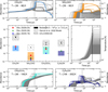 |
Fig. 8 Comparison between the model and observations of G328.25, G335.58 and G335.78. Middle left: lower and upper bounds of the model that best cover the observations at a given time of 6 × 10⁴ yr with a grain size of 0.5 μm. These areas of best coverage relate to various locations in the envelope; they are marked by the lines in the top and bottom panels, which are colour-coded by temperature. Comparisons with the 0D model (UCLCHEM-0D with G0=1 and Garrod et al. 2022) are also provided; mean prediction values are shown with ‘x’ symbols and asterisks, while the hatched lines boxes mark a factor of 5 scatter around these mean values. Middle right: temperature profile for all locations in our model. |
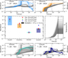 |
Fig. 9 Similar to Figure 8 but with observations of the Orion hot core for CH3OH, CH3OCH3, HCOOH, and C2H5OH towards MF, EG, and ET peaks at a specific cloud age of 6 × 10⁴ yr. Our model underestimates the X(C2H5OH) observed in the ET peak. |
Acknowledgements
This work is financially supported by the advanced ERC grant (ID: 833460, PI: Serena Viti) within the framework of MOlecules as Probes of the Physics of EXternal (MOPPEX) project. AC received financial support from the ERC Starting Grant “Chemtrip” (grant agreement No. 949278). T.H. acknowledges the support from the main research project (No. 2025186902) from Korea Astronomy and Space Science Institute (KASI).
References
- Agúndez, M., Marcelino, N., Tercero, B., et al. 2021, A&A, 649, L4 [NASA ADS] [CrossRef] [EDP Sciences] [Google Scholar]
- Awad, Z., Viti, S., Collings, M. P., & Williams, D. A. 2010, MNRAS, 407, 2511 [Google Scholar]
- Barone, V., Latouche, C., Skouteris, D., et al. 2015, MNRAS, 453, L31 [Google Scholar]
- Belloche, A., Menten, K. M., Comito, C., et al. 2008, A&A, 482, 179 [NASA ADS] [CrossRef] [EDP Sciences] [Google Scholar]
- Belloche, A., Garrod, R. T., Müller, H. S. P., et al. 2019, A&A, 628, A10 [NASA ADS] [CrossRef] [EDP Sciences] [Google Scholar]
- Bonfand, M., Belloche, A., Menten, K. M., Garrod, R. T., & Müller, H. S. P. 2017, A&A, 604, A60 [NASA ADS] [CrossRef] [EDP Sciences] [Google Scholar]
- Bonfand, M., Belloche, A., Garrod, R. T., et al. 2019, A&A, 628, A27 [NASA ADS] [CrossRef] [EDP Sciences] [Google Scholar]
- Bonnor, W. B. 1956, MNRAS, 116, 351 [NASA ADS] [CrossRef] [Google Scholar]
- Bouscasse, L., Csengeri, T., Wyrowski, F., Menten, K. M., & Bontemps, S. 2024, A&A, 686, A252 [NASA ADS] [CrossRef] [EDP Sciences] [Google Scholar]
- Busch, L. A., Belloche, A., Garrod, R. T., Müller, H. S. P., & Menten, K. M. 2022, A&A, 665, A96 [NASA ADS] [CrossRef] [EDP Sciences] [Google Scholar]
- Cardelli, J. A., Clayton, G. C., & Mathis, J. S. 1989, ApJ, 345, 245 [Google Scholar]
- Ceccarelli, C., Loinard, L., Castets, A., Tielens, A. G. G. M., & Caux, E. 2000, A&A, 357, L9 [NASA ADS] [Google Scholar]
- Ceccarelli, C., Codella, C., Balucani, N., et al. 2023, in Astronomical Society of the Pacific Conference Series, 534, Protostars and Planets VII, eds. S. Inutsuka, Y. Aikawa, T. Muto, K. Tomida, & M. Tamura, 379 [Google Scholar]
- Chang, Q., Cuppen, H. M., & Herbst, E. 2007, A&A, 469, 973 [NASA ADS] [CrossRef] [EDP Sciences] [Google Scholar]
- Choudhury, R., Schilke, P., Stéphan, G., et al. 2015, A&A, 575, A68 [NASA ADS] [CrossRef] [EDP Sciences] [Google Scholar]
- Coutens, A., Jørgensen, J. K., van der Wiel, M. H. D., et al. 2016, A&A, 590, L6 [NASA ADS] [CrossRef] [EDP Sciences] [Google Scholar]
- Cummins, S. E., Linke, R. A., & Thaddeus, P. 1986, ApJS, 60, 819 [NASA ADS] [CrossRef] [Google Scholar]
- Draine, B. T. 2011, Physics of the Interstellar and Intergalactic Medium [Google Scholar]
- Dutkowska, K. M., Vermariën, G., Viti, S., et al. 2025, A&A, 703, A46 [NASA ADS] [CrossRef] [EDP Sciences] [Google Scholar]
- Garrod, R. T., Widicus Weaver, S. L., & Herbst, E. 2008, ApJ, 682, 283 [Google Scholar]
- Garrod, R. T., Jin, M., Matis, K. A., et al. 2022, ApJS, 259, 1 [NASA ADS] [CrossRef] [Google Scholar]
- Goicoechea, J. R., Rodríguez-Fernández, N. J., & Cernicharo, J. 2004, ApJ, 600, 214 [CrossRef] [Google Scholar]
- Herbst, E., & van Dishoeck, E. F. 2009, ARA&A, 47, 427 [NASA ADS] [CrossRef] [Google Scholar]
- Hoang, T. 2021, ApJ, 921, 21 [NASA ADS] [CrossRef] [Google Scholar]
- Hoang, T., Lazarian, A., & Schlickeiser, R. 2015, ApJ, 806, 255 [NASA ADS] [CrossRef] [Google Scholar]
- Holdship, J., Viti, S., Jiménez-Serra, I., Makrymallis, A., & Priestley, F. 2017, AJ, 154, 38 [NASA ADS] [CrossRef] [Google Scholar]
- Ivlev, A. V., Silsbee, K., Sipilä, O., & Caselli, P. 2019, ApJ, 884, 176 [Google Scholar]
- Jiménez-Serra, I., Vasyunin, A. I., Caselli, P., et al. 2016, ApJ, 830, L6 [Google Scholar]
- Jørgensen, J. K., Favre, C., Bisschop, S. E., et al. 2012, ApJ, 757, L4 [Google Scholar]
- Martín-Doménech, R., Rivilla, V. M., Jiménez-Serra, I., et al. 2017, MNRAS, 469, 2230 [Google Scholar]
- Millar, T. J., Walsh, C., Van de Sande, M., & Markwick, A. J. 2024, A&A, 682, A109 [NASA ADS] [CrossRef] [EDP Sciences] [Google Scholar]
- Nomura, H., & Millar, T. J. 2004, A&A, 414, 409 [CrossRef] [EDP Sciences] [Google Scholar]
- O’Donoghue, R., Viti, S., Padovani, M., & James, T. 2022, ApJ, 934, 63 [Google Scholar]
- Priestley, F. D., Viti, S., & Williams, D. A. 2018, AJ, 156, 51 [NASA ADS] [CrossRef] [Google Scholar]
- Quénard, D., Jiménez-Serra, I., Viti, S., Holdship, J., & Coutens, A. 2018, MNRAS, 474, 2796 [Google Scholar]
- Requena-Torres, M. A., Martín-Pintado, J., Martín, S., & Morris, M. R. 2008, ApJ, 672, 352 [Google Scholar]
- Sabatini, G., Bovino, S., Giannetti, A., et al. 2021, A&A, 652, A71 [NASA ADS] [CrossRef] [EDP Sciences] [Google Scholar]
- Schwörer, A., Sánchez-Monge, Á., Schilke, P., et al. 2019, A&A, 628, A6 [NASA ADS] [CrossRef] [EDP Sciences] [Google Scholar]
- Skouteris, D., Vazart, F., Ceccarelli, C., et al. 2017, MNRAS, 468, L1 [NASA ADS] [Google Scholar]
- Tercero, B., Cuadrado, S., López, A., et al. 2018, A&A, 620, L6 [NASA ADS] [CrossRef] [EDP Sciences] [Google Scholar]
- van Dishoeck, E. F. 2014, Faraday Discuss., 168, 9 [NASA ADS] [CrossRef] [Google Scholar]
- Vastel, C., Ceccarelli, C., Lefloch, B., & Bachiller, R. 2014, ApJ, 795, L2 [NASA ADS] [CrossRef] [Google Scholar]
- Viti, S., & Williams, D. A. 1999, MNRAS, 305, 755 [NASA ADS] [CrossRef] [Google Scholar]
- Viti, S., Collings, M. P., Dever, J. W., McCoustra, M. R. S., & Williams, D. A. 2004, MNRAS, 354, 1141 [NASA ADS] [CrossRef] [Google Scholar]
Our Tthreshold is also known as Tsub in Hoang (2021) and the references therein.
The predicted abundances are adopted from Table 17 in Garrod et al. (2022, indicated by hatched areas).
Appendix A Mean wavelength of radiation fields from the protostar and hot dust shell
Figure A.1 illustrates how the mean wavelength of the radiation field changes as it moves away from the source. UV photons released by massive protostars are mostly absorbed, allowing longer-wavelength photons to propagate. In contrast, photons of longer wavelengths emitted by low-mass protostars can reach further into distant regions. Nevertheless, compared to the radiation field generated by the hot dust shell, the hot shell notably influences the radiation and then the temperature within the envelope.
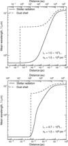 |
Fig. A.1 Decomposition of the radial profile of the radiation mean wavelength. The short-wavelength photons from the stellar radiations are effectively absorbed by the dust shell, allowing the longer-wavelength photons to penetrate to the outer region. The thermal radiation from the dust shell dominantly heats the outer region. |
Appendix B Radial profile of the cosmic-ray ionisation rate in the SgrB2(N1) hot core
Figure B.1 shows the best profile of the cosmic-ray ionisation rate w.r.t distance from the central source, in the SgrB2(N1) hot core. This profile is based on the best ζscale = 30 for the westward direction and ζscale = 20 for the southward direction. At 0.2 pc away from the centre, a higher rate is seen with ζ ≃ 50–60 × ζISM. This high number is consistent with Bonfand et al. (2019).
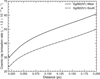 |
Fig. B.1 Radial profile of the comis-ray ionisation rate in the SgrB2(N1) hot core, inferred from the best models shown in Figure 7. The higher cosmic-ray ionisation rate is required in both directions, westwards and southwards. |
Appendix C Effect of grain size and UV radiation field
Figure C.1 illustrates the time variation in the abundances for a different location in the cloud (indicated by coloured lines) and grain sizes. Closer to the central light source, a rapid increase in abundance is observed as a result of, relatively high temperature compared to locations father into the cloud. These abundances are then compared with the above-mentioned data (black horizontal lines). Thus, to explain the observed data, CH3OH and NH2CHO must be emitted further away from the centre, while CH3OCH3 and C2H5OH originate nearer to the centre. Furthermore, when the grain size is 0.1 μm, our model underestimates the abundance of C2H5OH. By increasing the grain size to 0.5 μm and 1 μm, we find that to match the observed abundance of all COMs (including C2H5OH), the average grain size must be around 0.5 μm. This value is larger than the typical grain size in the diffuse ISM.
Figure C.2 shows the abundance of COMs at G0 = 10, as determined by the UCLCHEM-0D model. In contrast to the scenario of G0 = 1, the COMs exhibit significantly reduced abundances. Consequently, employing the 0D model can lead to a deficiency of UV-related processes in protostars due to the rapid attenuation of external UV radiation. Conversely, the 1D model highlights the significant influence of the central source’s internal UV field.
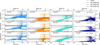 |
Fig. C.1 Time-dependent behaviour of COMs (lines, colour-coded by distance as in Figure 5) compared with measurements (horizontal black lines) taken from three infrared-quiet massive galactic clumps (G328.25, G335.58, and G335.78) with L = 104 L⊙. To better explain all the COM abundances reported for G335.58 (including C2H5OH), the average grain size is shown to be larger than the typical grain size of 0.1 μm in the diffuse ISM. |
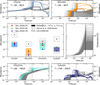 |
Fig. C.2 Similar to Figure 8 but the UCLCHEM-0D models for G0 = 10. The COMs are less abundant for higher values of the UV radiation field. |
All Tables
Total initial elemental abundances with respect to the total number of hydrogen nuclei (H).
Key physical parameters for the modelling along the west and south directions of the SgrB2(N1) hot core.
All Figures
|
Fig. 1 Sketch of the protostellar core adopted in this model, including a central source characterised by the bolometric luminosity (L*) and the stellar temperature (T*). The inner zone is characterised by the sublimation threshold of dust grains (Tsub) and the threshold radius (rthreshold). The thin shell of hot dust is determined by the shell temperature (Tshell) and its radius (Rshell). The outer region is given by the outer radius (rout). |
| In the text | |
|
Fig. 2 Variations in stellar and dust shell radiations with respect to radial distance for low-mass (left panel) and high-mass (right panel) protostellar cores. For r < rthreshold (marked by the vertical dashed-dotted line), the stellar radiation decreases as U(T*, nodust) ~r−2. For r > rthreshold, this stellar radiation (U(T*)) is quickly reduced because of dust attenuation. The radiation in the outer region is mainly dominated by the emission from the dust shell (U(Tshell)). |
| In the text | |
|
Fig. 3 Examples of radial profiles of the gas density (solid line, left y-axis) and dust temperature (dashed line, right y-axis) in protostars of different L* embedded in a molecular core for r ≥ rthreshold. In each panel, our temperature profile is compared to the profiles found in the literature. For the profiles from Sabatini et al. (2021), we used n0 = 107 cm−3 and r0 = 0.15 pc, the same as the authors. For the profile from Nomura & Millar (2004), we used n0 = 1.5 × 106 cm−3 and r0 = 0.05 pc. |
| In the text | |
|
Fig. 4 Examples of the profiles of the gas density (top), visual extinction from the surface (middle) and temperature (bottom). The negative time is for the pre-stellar phase, and a time of zero is when the protostar is formed. For visualisation purposes, 50 of the 100 gas parcels in the sampling are shown. The values of ngas(r) estimated by Eq. (1) and the Td(r) estimated by Eq. (9) are the final values of ngas(t) in Eq. (10) and Td(t) in Eq. (13) at a given location r. These profiles have L* = 105 L⊙, nin = 107 cm−3, rflat=0.05 pc and a = 0.5 μm. |
| In the text | |
|
Fig. 5 Example of the variation in CH3OH with time for L* = 100 L⊙ (left) and L* = 105 L⊙ (right). Lines are for the 100 parcels (full grid) from the center, color-coded by the temperature at t = 106 yr. The abundance of CH3OH decreases sharply at late times because of the reaction with neutral and ion species. For instance, at t = 5 × 10⁵ yr, the most important destruction reactions are H3O+ + CH3OH → CH3OH2+ + H2O and H3+ + CH3OH → CH3+ + H2O + H2. |
| In the text | |
|
Fig. 6 Abundance of various COMs as a function of distance based on different source luminosities at different ages. While the chosen age is arbitrary, it is consistent with the fact that a more massive protostar evolves faster than the less massive one. Typically, the abundance remains unchanged near the centre and decreases farther out. In the case of a more massive protostellar core, the abundance extends over a larger volume. |
| In the text | |
|
Fig. 7 Radial profiles of some COMs as a function of radial distance moving westwards (left panel) and southwards (right panel) from the SgrB2(N1) hot core with G0 = 103. The symbols represent observational data. The prominent solid lines illustrate the best models (the lighter lines denote models corresponding to the ages within ±1σ around the age determined by the best χ2). Our model can nicely reproduce the radial profiles of CH3OH, CH3OCH3, NH2CHO and CH3CHO but fails to explain the C2H5OH profile. To better match observations for all COMs, the cosmic ray ionisation rate is required to be higher than the typical value of the ISM. For the westwards, ζscale = 30 corresponds to ζ(0.2 pc) ≃ 60 × ζISRF, and ζscale = 20 corresponds to ζ(0.2 pc) ≃ 50 × ζISRF for the southwards. The best-fit period correspond to (3–7) × 104 yr. |
| In the text | |
|
Fig. 8 Comparison between the model and observations of G328.25, G335.58 and G335.78. Middle left: lower and upper bounds of the model that best cover the observations at a given time of 6 × 10⁴ yr with a grain size of 0.5 μm. These areas of best coverage relate to various locations in the envelope; they are marked by the lines in the top and bottom panels, which are colour-coded by temperature. Comparisons with the 0D model (UCLCHEM-0D with G0=1 and Garrod et al. 2022) are also provided; mean prediction values are shown with ‘x’ symbols and asterisks, while the hatched lines boxes mark a factor of 5 scatter around these mean values. Middle right: temperature profile for all locations in our model. |
| In the text | |
|
Fig. 9 Similar to Figure 8 but with observations of the Orion hot core for CH3OH, CH3OCH3, HCOOH, and C2H5OH towards MF, EG, and ET peaks at a specific cloud age of 6 × 10⁴ yr. Our model underestimates the X(C2H5OH) observed in the ET peak. |
| In the text | |
|
Fig. A.1 Decomposition of the radial profile of the radiation mean wavelength. The short-wavelength photons from the stellar radiations are effectively absorbed by the dust shell, allowing the longer-wavelength photons to penetrate to the outer region. The thermal radiation from the dust shell dominantly heats the outer region. |
| In the text | |
|
Fig. B.1 Radial profile of the comis-ray ionisation rate in the SgrB2(N1) hot core, inferred from the best models shown in Figure 7. The higher cosmic-ray ionisation rate is required in both directions, westwards and southwards. |
| In the text | |
|
Fig. C.1 Time-dependent behaviour of COMs (lines, colour-coded by distance as in Figure 5) compared with measurements (horizontal black lines) taken from three infrared-quiet massive galactic clumps (G328.25, G335.58, and G335.78) with L = 104 L⊙. To better explain all the COM abundances reported for G335.58 (including C2H5OH), the average grain size is shown to be larger than the typical grain size of 0.1 μm in the diffuse ISM. |
| In the text | |
|
Fig. C.2 Similar to Figure 8 but the UCLCHEM-0D models for G0 = 10. The COMs are less abundant for higher values of the UV radiation field. |
| In the text | |
Current usage metrics show cumulative count of Article Views (full-text article views including HTML views, PDF and ePub downloads, according to the available data) and Abstracts Views on Vision4Press platform.
Data correspond to usage on the plateform after 2015. The current usage metrics is available 48-96 hours after online publication and is updated daily on week days.
Initial download of the metrics may take a while.