| Issue |
A&A
Volume 708, April 2026
|
|
|---|---|---|
| Article Number | A105 | |
| Number of page(s) | 19 | |
| Section | Cosmology (including clusters of galaxies) | |
| DOI | https://doi.org/10.1051/0004-6361/202556642 | |
| Published online | 30 March 2026 | |
Euclid preparation
LXXXVII. Non-Gaussianity of two-point statistics likelihood: Precise analysis of the matter power spectrum distribution
1
Aix-Marseille Université, Université de Toulon, CNRS, CPT, Marseille, France
2
Institut d’Estudis Espacials de Catalunya (IEEC), Edifici RDIT, Campus UPC, 08860 Castelldefels, Barcelona, Spain
3
Institute of Space Sciences (ICE, CSIC), Campus UAB, Carrer de Can Magrans, s/n, 08193 Barcelona, Spain
4
Aix-Marseille Université, CNRS/IN2P3, CPPM, Marseille, France
5
Aix Marseille Univ, INSERM, MMG, Marseille, France
6
Center for Data-Driven Discovery, Kavli IPMU (WPI), UTIAS, The University of Tokyo, Kashiwa, Chiba 277-8583, Japan
7
Laboratoire d’etude de l’Univers et des phenomenes eXtremes, Observatoire de Paris, Université PSL, Sorbonne Université, CNRS, 92190 Meudon, France
8
INAF-IASF Milano, Via Alfonso Corti 12, 20133 Milano, Italy
9
Institut d’Astrophysique de Paris, UMR 7095, CNRS, and Sorbonne Université, 98 bis boulevard Arago, 75014 Paris, France
10
INAF-Osservatorio Astronomico di Trieste, Via G. B. Tiepolo 11, 34143 Trieste, Italy
11
IFPU, Institute for Fundamental Physics of the Universe, Via Beirut 2, 34151 Trieste, Italy
12
INFN, Sezione di Trieste, Via Valerio 2, 34127 Trieste TS, Italy
13
School of Mathematics and Physics, University of Surrey, Guildford, Surrey GU2 7XH, UK
14
INAF-Osservatorio Astronomico di Brera, Via Brera 28, 20122 Milano, Italy
15
INAF-Osservatorio di Astrofisica e Scienza dello Spazio di Bologna, Via Piero Gobetti 93/3, 40129 Bologna, Italy
16
SISSA, International School for Advanced Studies, Via Bonomea 265, 34136 Trieste TS, Italy
17
Dipartimento di Fisica e Astronomia, Università di Bologna, Via Gobetti 93/2, 40129 Bologna, Italy
18
INFN-Sezione di Bologna, Viale Berti Pichat 6/2, 40127 Bologna, Italy
19
Dipartimento di Fisica, Università di Genova, Via Dodecaneso 33, 16146 Genova, Italy
20
INFN-Sezione di Genova, Via Dodecaneso 33, 16146 Genova, Italy
21
Department of Physics “E. Pancini”, University Federico II, Via Cinthia 6, 80126 Napoli, Italy
22
INAF-Osservatorio Astronomico di Capodimonte, Via Moiariello 16, 80131 Napoli, Italy
23
Instituto de Astrofísica e Ciências do Espaço, Universidade do Porto, CAUP, Rua das Estrelas, PT4150-762 Porto, Portugal
24
Faculdade de Ciências da Universidade do Porto, Rua do Campo de Alegre, 4150-007 Porto, Portugal
25
European Southern Observatory, Karl-Schwarzschild-Str. 2, 85748 Garching, Germany
26
Dipartimento di Fisica, Università degli Studi di Torino, Via P. Giuria 1, 10125 Torino, Italy
27
INFN-Sezione di Torino, Via P. Giuria 1, 10125 Torino, Italy
28
INAF-Osservatorio Astrofisico di Torino, Via Osservatorio 20, 10025 Pino Torinese (TO), Italy
29
European Space Agency/ESTEC, Keplerlaan 1, 2201 AZ, Noordwijk, The Netherlands
30
Institute Lorentz, Leiden University, Niels Bohrweg 2, 2333 CA, Leiden, The Netherlands
31
Leiden Observatory, Leiden University, Einsteinweg 55, 2333 CC, Leiden, The Netherlands
32
INAF-Osservatorio Astronomico di Roma, Via Frascati 33, 00078 Monteporzio Catone, Italy
33
INFN-Sezione di Roma, Piazzale Aldo Moro, 2 – c/o Dipartimento di Fisica, Edificio G. Marconi, 00185 Roma, Italy
34
Centro de Investigaciones Energéticas, Medioambientales y Tecnológicas (CIEMAT), Avenida Complutense 40, 28040 Madrid, Spain
35
Port d’Informació Científica, Campus UAB, C. Albareda s/n, 08193 Bellaterra (Barcelona), Spain
36
Institute for Theoretical Particle Physics and Cosmology (TTK), RWTH Aachen University, 52056 Aachen, Germany
37
INFN section of Naples, Via Cinthia 6, 80126 Napoli, Italy
38
Institute for Astronomy, University of Hawaii, 2680 Woodlawn Drive, Honolulu, HI 96822, USA
39
Dipartimento di Fisica e Astronomia “Augusto Righi” – Alma Mater Studiorum Università di Bologna, Viale Berti Pichat 6/2, 40127 Bologna, Italy
40
Instituto de Astrofísica de Canarias, Vía Láctea, 38205 La Laguna, Tenerife, Spain
41
Institute for Astronomy, University of Edinburgh, Royal Observatory, Blackford Hill, Edinburgh EH9 3HJ, UK
42
Jodrell Bank Centre for Astrophysics, Department of Physics and Astronomy, University of Manchester, Oxford Road, Manchester M13 9PL, UK
43
European Space Agency/ESRIN, Largo Galileo Galilei 1, 00044 Frascati, Roma, Italy
44
ESAC/ESA, Camino Bajo del Castillo, s/n., Urb. Villafranca del Castillo, 28692 Villanueva de la Cañada, Madrid, Spain
45
Université Claude Bernard Lyon 1, CNRS/IN2P3, IP2I Lyon, UMR 5822, Villeurbanne F-69100, France
46
Aix-Marseille Université, CNRS, CNES, LAM, Marseille, France
47
Institut de Ciències del Cosmos (ICCUB), Universitat de Barcelona (IEEC-UB), Martí i Franquès 1, 08028 Barcelona, Spain
48
Institució Catalana de Recerca i Estudis Avançats (ICREA), Passeig de Lluís Companys 23, 08010 Barcelona, Spain
49
UCB Lyon 1, CNRS/IN2P3, IUF, IP2I Lyon, 4 rue Enrico Fermi, 69622 Villeurbanne, France
50
Departamento de Física, Faculdade de Ciências, Universidade de Lisboa, Edifício C8, Campo Grande, PT1749-016 Lisboa, Portugal
51
Instituto de Astrofísica e Ciências do Espaço, Faculdade de Ciências, Universidade de Lisboa, Campo Grande, 1749-016 Lisboa, Portugal
52
Department of Astronomy, University of Geneva, ch. d’Ecogia 16, 1290 Versoix, Switzerland
53
INAF-Istituto di Astrofisica e Planetologia Spaziali, Via del Fosso del Cavaliere, 100, 00100 Roma, Italy
54
Space Science Data Center, Italian Space Agency, Via del Politecnico snc, 00133 Roma, Italy
55
INFN-Bologna, Via Irnerio 46, 40126 Bologna, Italy
56
Universitäts-Sternwarte München, Fakultät für Physik, Ludwig-Maximilians-Universität München, Scheinerstrasse 1, 81679 München, Germany
57
Max Planck Institute for Extraterrestrial Physics, Giessenbachstr. 1, 85748 Garching, Germany
58
INAF-Osservatorio Astronomico di Padova, Via dell’Osservatorio 5, 35122 Padova, Italy
59
Dipartimento di Fisica “Aldo Pontremoli”, Università degli Studi di Milano, Via Celoria 16, 20133 Milano, Italy
60
INFN-Sezione di Milano, Via Celoria 16, 20133 Milano, Italy
61
Institute of Theoretical Astrophysics, University of Oslo, P.O. Box 1029 Blindern, 0315 Oslo, Norway
62
Jet Propulsion Laboratory, California Institute of Technology, 4800 Oak Grove Drive, Pasadena, CA 91109, USA
63
Felix Hormuth Engineering, Goethestr. 17, 69181 Leimen, Germany
64
Technical University of Denmark, Elektrovej 327, 2800 Kgs. Lyngby, Denmark
65
Cosmic Dawn Center (DAWN), Denmark
66
Max-Planck-Institut für Astronomie, Königstuhl 17, 69117 Heidelberg, Germany
67
NASA Goddard Space Flight Center, Greenbelt, MD 20771, USA
68
Department of Physics and Astronomy, University College London, Gower Street, London WC1E 6BT, UK
69
Department of Physics and Helsinki Institute of Physics, Gustaf Hällströmin katu 2, 00014 University of Helsinki, Finland
70
Université de Genève, Département de Physique Théorique and Centre for Astroparticle Physics, 24 quai Ernest-Ansermet, CH-1211 Genève 4, Switzerland
71
Department of Physics, P.O. Box 64, 00014 University of Helsinki, Finland
72
Helsinki Institute of Physics, Gustaf Hällströmin katu 2, University of Helsinki, Helsinki, Finland
73
SKA Observatory, Jodrell Bank, Lower Withington, Macclesfield, Cheshire SK11 9FT, UK
74
Centre de Calcul de l’IN2P3/CNRS, 21 avenue Pierre de Coubertin, 69627 Villeurbanne Cedex, France
75
Universität Bonn, Argelander-Institut für Astronomie, Auf dem Hügel 71, 53121 Bonn, Germany
76
Dipartimento di Fisica e Astronomia “Augusto Righi” – Alma Mater Studiorum Università di Bologna, Via Piero Gobetti 93/2, 40129 Bologna, Italy
77
Department of Physics, Institute for Computational Cosmology, Durham University, South Road, Durham DH1 3LE, UK
78
Institut d’Astrophysique de Paris, 98bis Boulevard Arago, 75014 Paris, France
79
Institute of Physics, Laboratory of Astrophysics, Ecole Polytechnique Fédérale de Lausanne (EPFL), Observatoire de Sauverny, 1290 Versoix, Switzerland
80
Telespazio UK S.L. for European Space Agency (ESA), Camino bajo del Castillo, s/n, Urbanizacion Villafranca del Castillo, Villanueva de la Cañada, 28692, Madrid, Spain
81
Institut de Física d’Altes Energies (IFAE), The Barcelona Institute of Science and Technology, Campus UAB, 08193 Bellaterra (Barcelona), Spain
82
DARK, Niels Bohr Institute, University of Copenhagen, Jagtvej 155, 2200 Copenhagen, Denmark
83
Waterloo Centre for Astrophysics, University of Waterloo, Waterloo, Ontario N2L 3G1, Canada
84
Department of Physics and Astronomy, University of Waterloo, Waterloo, Ontario N2L 3G1, Canada
85
Perimeter Institute for Theoretical Physics, Waterloo, Ontario N2L 2Y5, Canada
86
Université Paris-Saclay, Université Paris Cité, CEA, CNRS, AIM, 91191 Gif-sur-Yvette, France
87
Centre National d’Etudes Spatiales – Centre spatial de Toulouse, 18 avenue Edouard Belin, 31401 Toulouse Cedex 9, France
88
Institute of Space Science, Str. Atomistilor, nr. 409 Măgurele, Ilfov 077125, Romania
89
Dipartimento di Fisica e Astronomia “G. Galilei”, Università di Padova, Via Marzolo 8, 35131 Padova, Italy
90
INFN-Padova, Via Marzolo 8, 35131 Padova, Italy
91
Institut für Theoretische Physik, University of Heidelberg, Philosophenweg 16, 69120 Heidelberg, Germany
92
Institut de Recherche en Astrophysique et Planétologie (IRAP), Université de Toulouse, CNRS, UPS, CNES, 14 Av. Edouard Belin, 31400 Toulouse, France
93
Université St Joseph; Faculty of Sciences, Beirut, Lebanon
94
Departamento de Física, FCFM, Universidad de Chile, Blanco Encalada, 2008 Santiago, Chile
95
Universität Innsbruck, Institut für Astro- und Teilchenphysik, Technikerstr. 25/8, 6020 Innsbruck, Austria
96
Satlantis, University Science Park, Sede Bld, 48940 Leioa-Bilbao, Spain
97
Instituto de Astrofísica e Ciências do Espaço, Faculdade de Ciências, Universidade de Lisboa, Tapada da Ajuda, 1349-018 Lisboa, Portugal
98
Cosmic Dawn Center (DAWN)
99
Niels Bohr Institute, University of Copenhagen, Jagtvej 128, 2200 Copenhagen, Denmark
100
Universidad Politécnica de Cartagena, Departamento de Electrónica y Tecnología de Computadoras, Plaza del Hospital 1, 30202 Cartagena, Spain
101
Infrared Processing and Analysis Center, California Institute of Technology, Pasadena, CA 91125, USA
102
Dipartimento di Fisica e Scienze della Terra, Università degli Studi di Ferrara, Via Giuseppe Saragat 1, 44122 Ferrara, Italy
103
Istituto Nazionale di Fisica Nucleare, Sezione di Ferrara, Via Giuseppe Saragat 1, 44122 Ferrara, Italy
104
INAF, Istituto di Radioastronomia, Via Piero Gobetti 101, 40129 Bologna, Italy
105
Astronomical Observatory of the Autonomous Region of the Aosta Valley (OAVdA), Loc. Lignan 39, I-11020 Nus (Aosta Valley), Italy
106
Department of Physics, Oxford University, Keble Road, Oxford OX1 3RH, UK
107
Aurora Technology for European Space Agency (ESA), Camino bajo del Castillo, s/n, Urbanizacion Villafranca del Castillo, Villanueva de la Cañada, 28692, Madrid, Spain
108
ICL, Junia, Université Catholique de Lille, LITL, 59000 Lille, France
109
ICSC – Centro Nazionale di Ricerca in High Performance Computing, Big Data e Quantum Computing, Via Magnanelli 2, Bologna, Italy
110
Instituto de Física Teórica UAM-CSIC, Campus de Cantoblanco, 28049 Madrid, Spain
111
CERCA/ISO, Department of Physics, Case Western Reserve University, 10900 Euclid Avenue, Cleveland, OH 44106, USA
112
Technical University of Munich, TUM School of Natural Sciences, Physics Department, James-Franck-Str. 1, 85748 Garching, Germany
113
Max-Planck-Institut für Astrophysik, Karl-Schwarzschild-Str. 1, 85748 Garching, Germany
114
Laboratoire Univers et Théorie, Observatoire de Paris, Université PSL, Université Paris Cité, CNRS, 92190 Meudon, France
115
Departamento de Física Fundamental. Universidad de Salamanca, Plaza de la Merced s/n., 37008 Salamanca, Spain
116
Université de Strasbourg, CNRS, Observatoire astronomique de Strasbourg, UMR 7550, 67000 Strasbourg, France
117
Dipartimento di Fisica – Sezione di Astronomia, Università di Trieste, Via Tiepolo 11, 34131 Trieste, Italy
118
California Institute of Technology, 1200 E California Blvd, Pasadena, CA 91125, USA
119
Department of Physics & Astronomy, University of California Irvine, Irvine, CA 92697, USA
120
Kapteyn Astronomical Institute, University of Groningen, PO Box 800, 9700 AV, Groningen, The Netherlands
121
Departamento Física Aplicada, Universidad Politécnica de Cartagena, Campus Muralla del Mar, 30202 Cartagena, Murcia, Spain
122
Instituto de Física de Cantabria, Edificio Juan Jordá, Avenida de los Castros, 39005 Santander, Spain
123
INFN, Sezione di Lecce, Via per Arnesano, CP-193, 73100 Lecce, Italy
124
Department of Mathematics and Physics E. De Giorgi, University of Salento, Via per Arnesano, CP-I93, 73100 Lecce, Italy
125
INAF-Sezione di Lecce, c/o Dipartimento Matematica e Fisica, Via per Arnesano, 73100 Lecce, Italy
126
Université Paris Cité, CNRS, Astroparticule et Cosmologie, 75013 Paris, France
127
CEA Saclay, DFR/IRFU, Service d’Astrophysique, Bat. 709, 91191 Gif-sur-Yvette, France
128
Institute of Cosmology and Gravitation, University of Portsmouth, Portsmouth PO1 3FX, UK
129
Department of Computer Science, Aalto University, PO Box 15400 Espoo FI-00 076, Finland
130
Instituto de Astrofísica de Canarias, c/ Via Lactea s/n, La Laguna 38200, Spain. Departamento de Astrofísica de la Universidad de La Laguna, Avda. Francisco Sanchez, La Laguna, 38200, Spain
131
Universidad de La Laguna, Departamento de Astrofísica, 38206 La Laguna, Tenerife, Spain
132
Ruhr University Bochum, Faculty of Physics and Astronomy, Astronomical Institute (AIRUB), German Centre for Cosmological Lensing (GCCL), 44780 Bochum, Germany
133
Department of Physics and Astronomy, Vesilinnantie 5, 20014 University of Turku, Finland
134
Serco for European Space Agency (ESA), Camino bajo del Castillo, s/n, Urbanizacion Villafranca del Castillo, Villanueva de la Cañada, 28692, Madrid, Spain
135
ARC Centre of Excellence for Dark Matter Particle Physics, Melbourne, Australia
136
Centre for Astrophysics & Supercomputing, Swinburne University of Technology, Hawthorn, Victoria 3122, Australia
137
Department of Physics and Astronomy, University of the Western Cape, Bellville, Cape Town, 7535, South Africa
138
DAMTP, Centre for Mathematical Sciences, Wilberforce Road, Cambridge CB3 0WA, UK
139
Kavli Institute for Cosmology Cambridge, Madingley Road, Cambridge CB3 0HA, UK
140
Department of Astrophysics, University of Zurich, Winterthurerstrasse 190, 8057 Zurich, Switzerland
141
Department of Physics, Centre for Extragalactic Astronomy, Durham University, South Road, Durham DH1 3LE, UK
142
IRFU, CEA, Université Paris-Saclay, 91191 Gif-sur-Yvette Cedex, France
143
Univ. Grenoble Alpes, CNRS, Grenoble INP, LPSC-IN2P3, 53, Avenue des Martyrs, 38000 Grenoble, France
144
INAF-Osservatorio Astrofisico di Arcetri, Largo E. Fermi 5, 50125 Firenze, Italy
145
Dipartimento di Fisica, Sapienza Università di Roma, Piazzale Aldo Moro 2, 00185 Roma, Italy
146
Centro de Astrofísica da Universidade do Porto, Rua das Estrelas, 4150-762 Porto, Portugal
147
Université Paris-Saclay, CNRS, Institut d’astrophysique spatiale, 91405 Orsay, France
148
HE Space for European Space Agency (ESA), Camino bajo del Castillo, s/n, Urbanizacion Villafranca del Castillo, Villanueva de la Cañada, 28692, Madrid, Spain
149
INAF – Osservatorio Astronomico d’Abruzzo, Via Maggini, 64100 Teramo, Italy
150
Theoretical astrophysics, Department of Physics and Astronomy, Uppsala University, Box 516, 751 37 Uppsala, Sweden
151
Mathematical Institute, University of Leiden, Einsteinweg 55, 2333 CA, Leiden, The Netherlands
152
Institute of Astronomy, University of Cambridge, Madingley Road, Cambridge CB3 0HA, UK
153
Univ. Lille, CNRS, Centrale Lille, UMR 9189 CRIStAL, 59000 Lille, France
154
Department of Astrophysical Sciences, Peyton Hall, Princeton University, Princeton, NJ 08544, USA
155
Space physics and astronomy research unit, University of Oulu, Pentti Kaiteran katu 1, FI-90014 Oulu, Finland
156
Institut de Physique Théorique, CEA, CNRS, Université Paris-Saclay, 91191 Gif-sur-Yvette Cedex, France
157
Center for Computational Astrophysics, Flatiron Institute, 162 5th Avenue, 10010 New York, NY, USA
★ Corresponding author: This email address is being protected from spambots. You need JavaScript enabled to view it.
Received:
29
July
2025
Accepted:
29
December
2025
Abstract
We investigate the non-Gaussian features in the distribution of the matter power spectrum multipoles. Using the COVMOS method, we generated 100 000 mock realisations of dark matter density fields in both real and redshift space across multiple redshifts and cosmological models. We derived an analytical framework linking the non-Gaussianity of the power spectrum distribution to higher-order statistics of the density field, including the trispectrum and pentaspectrum. We explored the effect of redshift-space distortions, the geometry of the survey, the Fourier binning, the integral constraint, and the shot noise on the skewness of the distribution of the power spectrum measurements. Our results demonstrate that the likelihood of the estimated matter power spectrum significantly deviates from a Gaussian assumption on non-linear scales, particularly at low redshift. This departure is primarily driven by the pentaspectrum contribution, which dominates over the trispectrum at intermediate scales. We also examined the impact of the finiteness of the survey geometry in the context of the Euclid mission, and we find that both the shape of the survey and the integral constraint amplify the skewness.
Key words: cosmological parameters / cosmology: observations / cosmology: theory / large-scale structure of Universe
© The Authors 2026
 Open Access article, published by EDP Sciences, under the terms of the Creative Commons Attribution License (https://creativecommons.org/licenses/by/4.0), which permits unrestricted use, distribution, and reproduction in any medium, provided the original work is properly cited.
This article is published in open access under the Subscribe to Open model. This email address is being protected from spambots. You need JavaScript enabled to view it. to support open access publication.
1. Introduction
In recent years, observational cosmology has experienced significant advancements with the emergence of next-generation galaxy surveys designed to probe larger cosmic volumes and smaller scales than ever before. Examples of such surveys include the Euclid mission (Euclid Collaboration: Mellier et al. 2025), the Vera C. Rubin Observatory Legacy Survey of Space and Time (LSST, Ivezić et al. 2019), and the Dark Energy Spectroscopic Instrument (DESI, DESI Collaboration 2016). These cutting-edge surveys will provide unprecedented insights into the structure and evolution of the Universe, making it increasingly important to develop more accurate and robust methodologies for data analysis. As we push the boundaries of observational capabilities, it is crucial that our methods of parameter inference can ensure that we can effectively extract valuable information from the wealth of data that will be gathered by these surveys.
Cosmological information is generally extracted from the analysis of two-point statistics of the fields under study. In real space, this is done with the two-point correlation function, and in Fourier space, it is done with the power spectrum. The latter is the case for state-of-the art analyses of the temperature and polarisation of the cosmic microwave background (CMB; Planck Collaboration VI 2020) or the large-scale structure (LSS) of the Universe, using galaxy clustering obtained through spectroscopic data (Gil-Marín et al. 2020; Bautista et al. 2021; DESI Collaboration 2025) or a combination of weak lensing and clustering obtained through photometric data (Abbott et al. 2022; Asgari et al. 2021; More et al. 2023).
To extract this cosmological information, we need to assume, a priory, what the distribution of our data is in order to model the likelihood function. A simple assumption that is commonly made for two-point statistics is that they follow a multivariate Gaussian distribution. However, we know that it is not the case, even for Gaussian fields such as the CMB. Indeed, the two-point statistics of a Gaussian field follows a χ2 distribution with a number of degrees of freedom equal to the number of independent modes at the considered scale. On large scales this number is low such that the χ2 distribution is far from being a Gaussian (Hamimeche & Lewis 2008).
Moreover, at intermediate scales (above 30 Mpc/h), such as those probed by the Euclid mission (Euclid Collaboration: Mellier et al. 2025), the non-linear clustering of matter generates non-vanishing N-point statistics (with N > 2) of the density field. A well-known consequence of the non-Gaussianity of the density field from the non-linear clustering of matter on the two-point statistics is the non-Gaussian contribution to the covariance matrix from a non-vanishing four-point correlation function (Scoccimarro et al. 1999). This higher-order contribution to the covariance is still present even though the likelihood is approximated to be Gaussian. In addition, these higher-order correlation functions also induce higher-order moments in the distribution of the two-point statistics, thus causing departure from the Gaussian assumption also at small scales. Indeed, the skewness and kurtosis of the two-point statistics distribution have been shown to be non-vanishing on small scales and especially at low redshift (Takahashi et al. 2009; Blot et al. 2015; Lin et al. 2020; Upham et al. 2021). Hall & Taylor (2022) also studied the potential influence of higher-order N-point statistics on the non-Gaussian distribution of two-point statistics on large scales in the context of a weak lensing likelihood analysis, but they found it to be negligible.
Given the precision with which we aim to measure the cosmological parameters with Euclid, we need to understand and control in detail the likelihood modelling and test whether it can significantly bias our cosmological analyses. Indeed, cosmological constraints derived from likelihood analysis generally rely on the assumption that the measurements are distributed according to a Gaussian. As a result, if the Gaussian assumption is not justified, it might affect the derived cosmological parameters. This is the aim of the present paper and its companion, Gouyou Beauchamps et al. (in prep., hereafter cited as GB-2025). In this work, we focus particularly on the Fourier version of two-point statistics, the power spectrum, to develop an analytical framework to understand how the non-Gaussianity of the two-point statistics distribution is linked to the non-Gaussianity of the field itself and what are the settings of the likelihood to which it is the most sensitive. In particular, we look at how the skewness and kurtosis of the distribution of the matter power spectrum changes with respect to (i) cosmological effects such as the cosmological model, the redshift, and the presence or absence of redshift space distortions (RSD); (ii) the settings of the power spectrum estimator, such as the presence of aliasing and the Fourier mode binning; and (iii) the effects originating from specific features of the survey, such as the sample density and the survey footprint. Our companion paper, GB-2025, specifically focuses on the impact of wrongly assuming a Gaussian likelihood on Euclid cosmological constraints.
To achieve all of this, we extensively rely on the COVMOS method (Baratta et al. 2020, 2023) in order to produce very large sets of approximate simulations of non-Gaussian fields, which allow us to precisely explore the distribution of the power spectrum. It has been shown in Baratta et al. (2023) that COVMOS is a reliable tool to model the covariance of two-point statistics, and we show in this paper that it is also the case for the study of their full distribution.
Since the main scope of the present paper is to understand the mechanisms possibly producing a non-Gaussian behaviour of the distribution of the estimated power spectrum, we focus on the matter field. In GB-2025, we use more realistic mock galaxy catalogues to study the skewness of the galaxy power spectrum. Finally, we note that this work does not aim to study the non-Gaussianity of the likelihood arising from the estimation of a covariance matrix with a low number of realisations (Sellentin & Heavens 2016; Percival et al. 2022).
The paper is structured as follows. In Sect. 2 we present our analytical framework to study the distribution of the power spectrum. In Sect. 3 we describe the simulation sets we constructed with COVMOS and introduce the estimators we applied on them. In Sect. 4 we study the estimated distribution of the power spectrum under various scenarios. In Sect. 5 we study the distribution of individual Fourier modes. Finally, we conclude in Sect. 6.
2. Skewness of the power spectrum estimator
In this section we derive the skewness of the probability distribution of the estimator of the power spectrum in terms of the higher-order N-points cumulant moments of the density field. We start with some definitions. The ensemble average of the random variable X following the probability density function (PDF) 𝒫 is ⟨X⟩, and ⟨X⟩c represents its connected expectation value. In practice, the random variable we study is the estimator of the multipoles of the power spectrum,  , defined as
 (1)
(1)
where ℓ refers to the order of the considered multipole, ℒℓ are the Legendre polynomials of order ℓ, k is the modulus of the considered spherical k-shell in Fourier space, Nk is the number of independent modes that it contains, μi is the cosine of the angle between the line of sight and the wave vector ki and the sum is made over independent modes inside the k-shell. Note that, by independent we do not mean statistically independent, but we rather refer to the fact that since the configuration space density field δ(x) is real, its Fourier space counterpart δ(k) satisfies  , where the ★ stands for complex conjugate. This means that there are repeated modes, that are not considered in Eq. (1). Unless otherwise stated, we consider a periodic boundary1conditions of size L, thus characterised by its fundamental mode kF := 2π/L. That is the reason why the sum in Eq. (1) is discrete. Finally, due to statistical invariance by translation (i.e. statistical homogeneity) one can define the power spectrum (P), the bispectrum (B), the trispectrum (T), and the pentaspectrum (Q) as
 (2)
(2)
 (3)
(3)
 (4)
(4)
 (5)
(5)
where we use the specific notation  for the Kronecker symbol, which is 1 if k1 + … + kN = 0 and 0 otherwise. To simplify the following calculations, we defined the random variables
  ,
,  and the coefficients
  . Thus, Xi depends on the wave vector k, and X depends on the wave mode k and on the chosen multipole ℓ. Based on these definitions, Eq. (1) takes the form
 (6)
(6)
Since the multi-point probability distribution function  of the modes Xi is not known, one can only focus on the cumulant moments in order to characterise how far from a Gaussian the distribution of X is. Indeed, if the variable X were following a Gaussian distribution then its cumulant moments should be ⟨Xn⟩c = 0 for n ≥ 3. Taking the ensemble average of Eq. (6) one can show that the mean of X is given by
 (7)
(7)
which means that the estimator is unbiased in the large Nk limit. We can then show that its variance is given by
 (8)
(8)
where the second sum is made over the Nk(Nk − 1)/2 permutations of i and j without repetitions. If the Fourier modes were statistically independent inside the shell then one could drop the double sum (second term) in Eq. (8). Notice that there is a subtlety that needs to be mentioned when inspecting Eq. (8), despite the fact that we define  one cannot say that
  . The equality holds only for the moments but not for the cumulant moments. Indeed, without paying attention to this, looking at Eq. (8) one would erroneously conclude that for a Gaussian field the variance of the shell average vanishes. Instead, one can use the relation between moments
  together with the assumption of statistical invariance by translation to show that for one-point statistics
 (9)
(9)
while for two-point statistics
 (10)
(10)
As a result, Eq. (8) ⟨XiXj⟩c involves a four-point function of the density field that is null in the Gaussian case. Instead, the first term of Eq. (8) contains an intrinsic contribution that would arise even if the density field were Gaussian (i.e.  ) and a part that would only arise when considering a non-Gaussian density field (i.e.
  ). The usual (see Scoccimarro et al. 1999; Meiksin & White 1999; Smith 2009; Smith & Marian 2015) expression for the variance of the power spectrum can be obtained by splitting ⟨Xi2⟩c (see Eq. (9)) into its Gaussian and non-Gaussian parts:
 (11)
(11)
where we define k as being at the centre of the spherical shell of thickness kF and Vk its volume. In addition, we define the shell average powers of the power spectrum as
 (12)
(12)
where the subscript Vk in the integral means that the integration variables belong to the Fourier shell, k, and thus  depends on the Fourier shell k. We note that we used the continuous limit of the shell average as described in the Appendix A. We also defined the corresponding quantity for the trispectrum as
 (13)
(13)
which also depends on the considered k-shell.
The same reasoning about moments and cumulant moments can be applied to obtain the formal expression of the skewness:
![Mathematical equation: $$ \begin{aligned} \langle X^3\rangle _{\rm c}&= \displaystyle \sum _{i = 1}^{N_k} a_i^3\langle X_i^3\rangle _{\rm c} + 3 \sum _{j>i}\left[ a_i^2 a_j \langle X_i^2 X_j\rangle _{\rm c} + a_i a_j^2 \langle X_i X_j^2\rangle _{\rm c} \right] \nonumber \\&\quad + 6 \displaystyle \sum _{n>j>i} a_ia_ja_n \langle X_i X_j X_n\rangle _{\rm c} . \end{aligned} $$](/articles/aa/full_html/2026/04/aa56642-25/aa56642-25-eq27.gif) (14)
(14)
Equation (14) allows us to understand that three kinds of correlators can contribute to the skewness, and they are
 (15)
(15)
 (16)
(16)
 (17)
(17)
The one-point cumulant (Eq. (15)) is composed of an intrinsic contribution (present even in the Gaussian case) and contributions related to the pentaspectrum and trispectrum. Then, there are two-point correlators (Eq. (16)) and three-point correlators (Eq. (17)) which would both be null in the Gaussian case since they involve only six- and four-point functions. By inserting Eqs. (15)–(17), into Eq. (14), one can express the full expression of the skewness as
 (18)
(18)
where we define the shell average of the square of the bispectrum as
 (19)
(19)
the shell average of the product between the power spectrum and the trispectrum as
 (20)
(20)
and the shell averaged pentaspectrum as
 (21)
(21)
In the present work we aim at quantifying the various terms involved in Eq. (18) and their relative contribution to the reduced skewness,
 (22)
(22)
in various configurations of the density field. In the rest of the paper we refer to the reduced skewness, S3(ℓ), as the skewness, where ℓ refers to the fact that this is the skewness of the multipole ℓ of the power spectrum2, and we refer to ⟨X3⟩c as the third-order cumulant.
3. Simulations and estimators
In this section we first present the different sets of simulations we generated and analysed in this study. Then, we present the different estimators employed to probe the distribution of the estimated power spectra.
3.1. Approximate simulations with COVMOS
The standard N-body approach is a widely used technique for simulating the evolution of large-scale cosmic structures. In our case, however, the computational cost of producing the large number of realisations required for a robust analysis of the power spectrum distribution is prohibitive. This is why in this study we exclusively rely on an approximate mock-catalogue generator, COVMOS3 (Baratta et al. 2020, 2023).
The COVMOS public code enables rapid simulation of catalogues for various cosmological objects in both real and redshift space. Its speed is due to the fact that it does not require the evolution of an initial density, as typically needed in an N-body process. Instead, a density field is directly generated at a specific redshift and then subjected to local Poisson sampling to create the point-like catalogue.
Although similar approaches, such as log-normal mock generators, are extensively studied in the literature (Xavier et al. 2016; Alonso et al. 2014; Agrawal et al. 2017), the COVMOS method has two distinctive features. First, the power spectrum of the density and velocity fields, as well as the density one-point PDF, can be arbitrarily set by the user. This flexibility means it is not restricted to a log-normal PDF, enabling the exploration of more realistic models. These statistics can be provided either from analytical models or directly from estimates based on simulations or observational data.
The second distinctive feature of the COVMOS method is its ability to assign specific velocities to objects based on the local density, while ensuring the validity of the continuity equation. This capability leads to a high simulation performance for RSD effects on two-point statistics, covering both the linear and mildly non-linear regimes.
The COVMOS method relies on the application of a local transform to a Gaussian field in order to match a target one-point PDF. As discussed in Baratta et al. (2023), this means that the higher order one-point moments of the PDF are correctly reproduced. Since they are given by specific integrals of the Fourier space N-point correlation functions, it is expected that COVMOS is able to capture some of the higher order information. Indeed, in Baratta et al. (2023) it has been shown that the non-Gaussian part of the covariance can be well recovered at least up to k ∼ 0.25 h/Mpc at z = 0. In addition, as shown in Sect. 2, the skewness of the distribution of the power spectrum depends on higher order correlation functions. This is the reason why we designed a validation procedure in Appendix B that justifies the use of the COVMOS method for this study.
In this study, we generated numerous large samples of dark matter catalogues in both real and redshift-space, all within simulated periodic boxes of volume 1 (Gpc/h)3. However, a cut in geometry of these catalogues, involving survey masks, is performed in Sect. 4.3.2. These samples are detailed in Table 1, which includes the sample name, simulated cosmology, and redshifts. Each sample contains 100 000 realisations of 108 particles, thus a density of 0.1 (Mpc/h)−3, this means that the shot-noise power spectrum is equal to the input power spectrum at k = 1.65 h/Mpc.
Redshift at which the COVMOS mock catalogue samples considered in this work have been generated.
We selected three different flat cosmologies compatible with the Planck 2013 results (Planck Collaboration XVI 2014), with cosmological parameters (Ωm, Ωb, h, ns, As = (0.32, 0.05, 0.67, 0.96, 2.1265 × 10⁻⁹). The first cosmology is characterised by a Lambda cold dark matter (ΛCDM) background, the second (16nu) includes massive neutrinos with total mass of ∑mν = 0.16 eV. In the third cosmology, named w9p3, a dynamical dark energy is included using the CPL (Chevallier & Polarski 2001; Linder 2003) parametrisation, where w(a) = w0 + wa(1 − a) and (w0, wa) = (−0.9, 0.3).
As previously stated, to use the COVMOS method, the user must specify target values for the power spectrum and one-point PDF of the density field, along with the target velocity power spectrum. For all our samples, we adopted these target values based on measurements performed in the DEMNUni suite of N-body simulations (Carbone et al. 2016) which have been run for the cosmological models described above. In the case of the ΛCDM and 16nu cosmology we use the one-point PDF and power spectrum, averaged over the 50 DEMNUni-Cov realisations (Baratta et al. 2023; Gouyou Beauchamps et al. 2025; Parimbelli et al. 2021), with a sampling of 512 points per side. For the w9p3 cosmology we use the unique realisation of this cosmological model from the DEMNUni set of simulations (Parimbelli et al. 2022) with a sampling of 1024 points per side (comoving box twice larger).
3.2. Statistics estimators
To estimate the power spectrum, we employed the widely used NBodyKit4 software (Hand et al. 2018), which offers robust and efficient tools for analysing the multipoles of the power spectrum, both in real and redshift space. In particular it allows the user to vary different settings of the estimation procedure, including the type of mass assignment scheme employed to interpolate particles on a grid, or the activation or not of the interlacing technique allowing the user to reduce the aliasing effect. We take advantage of this opportunity to identify a possible impact of these settings on the distribution of the output power spectra.
Despite having introduced (in Sect. 2) only the lowest level of non-Gaussianity (i.e. the skewness) of the distribution of the measured power spectrum, in the present work we also estimate the reduced kurtosis S4(ℓ) := ⟨X4⟩c/⟨X2⟩c2. We apply the same nomenclature to the kurtosis, i.e. S4(ℓ) is dubbed kurtosis, and ⟨X4⟩c is dubbed the fourth-order cumulant.
The estimation of the skewness and kurtosis is based on the Ns = 100 000 realisations that we generated with the COVMOS method, and their estimators are
![Mathematical equation: $$ \begin{aligned} \hat{S}_3^{(\ell )}(k) = \frac{N_{\rm s}^{-1}\sum _{i = 1}^{N_{\rm s}} \left[\hat{P}_i^{(\ell )} (k) - \bar{P}^{(\ell )}(k)\right]^3}{\left\{ N_{\rm s}^{-1}\sum _{i = 1}^{N_{\rm s}} \left[\hat{P}_i^{(\ell )} (k) - \bar{P}^{(\ell )}(k)\right]^2 \right\} ^{3/2}}\; \end{aligned} $$](/articles/aa/full_html/2026/04/aa56642-25/aa56642-25-eq36.gif) (23)
(23)
and
![Mathematical equation: $$ \begin{aligned} \hat{S}_4^{(\ell )}(k) = \frac{N_{\rm s}^{-1}\sum _{i = 1}^{N_{\rm s}} \left[\hat{P}_i^{(\ell )} (k) - \bar{P}^{(\ell )}(k)\right]^4}{\left\{ N_{\rm s}^{-1}\sum _{i = 1}^{N_{\rm s}} \left[\hat{P}_i^{(\ell )} (k) - \bar{P}^{(\ell )}(k)\right]^2 \right\} ^2} -3 , \end{aligned} $$](/articles/aa/full_html/2026/04/aa56642-25/aa56642-25-eq37.gif) (24)
(24)
where  is our estimate of the ℓ-th multipole of the power spectrum in shell k for the i-th COVMOS realisation, and
  is the estimated average multipole power spectrum over the Ns COVMOS realisations,
 (25)
(25)
Note that since we are estimating the mean  , the estimators of the skewness and kurtosis are expected to be biased. However, given the extremely high number of realisations, Ns, we can safely neglect that bias. Indeed, the variance would be affected at the level of Ns/(Ns − 1), and the skewness would be affected at the level of Ns2/(Ns − 2)/(Ns − 1) (i.e. adjusted Fisher–Pearson standardised moment coefficient), which is at most of the order of 0.3%.
The estimation of the skewness and kurtosis should be compared to the corresponding prediction assuming a Gaussian density field to quantify their excess. In Appendix A we review the general Gaussian field prediction for Sn(ℓ), which if one further assumes an isotropic real space power spectrum, it can be expressed as
 (26)
(26)
 (27)
(27)
for the monopole power spectrum estimator, where Nk is the number of independent wave modes in the considered k-shell. One can notice that Eqs. (26) and (27) apparently differ from Takahashi et al. (2009), but this is only due to a different definition of the number of modes, Nk. Indeed, they defined Nk as the total number of modes, while we restrict it to the independent modes (as previously explained). Thus, Nk can either be computed exactly on a Fourier grid or approximately evaluated analytically by dividing the total Fourier volume of the shell (2π k2 kF) by the Fourier volume (kF3) of an individual mode, yielding
 (28)
(28)
Note that Eqs. (26) and (27) are different when considering the quadrupole and the hexadecapole. We show in Appendix A that
 (29)
(29)
 (30)
(30)
 (31)
(31)
 (32)
(32)
In redshift space the expressions are more complicated but knowing the multipoles of the power spectrum one can still evaluate the corresponding expressions numerically on the 3D Fourier grid as given by Eq. (A.10) in Appendix A.
4. Quantifying the non-Gaussianity of the distribution of the estimated power spectrum
In this section we present a phenomenological study of the power spectrum distribution when varying different parameters. First, we study the cosmological effects that may impact the various statistics due to non-linear clustering. This includes the cosmological model and the redshift. Then, we investigate the effect of the power spectrum estimator’s settings through the Fourier mode binning and the NBodyKit input parameters for the 3D Fourier grid. Finally, we look at survey specific features, namely the sample density and the survey mask.
4.1. Cosmological effects
In this subsection we want to explore the potential cosmological factors that could influence the distribution of the power spectrum estimator, primarily as a result of non-linear clustering. Thanks to the analytical framework developed in Sect. 2 we are able to quantify the different terms contributing to the non-Gaussianity of the distribution.
In Fig. 1 we present the estimated skewness S3(ℓ) and kurtosis S4(ℓ) of the distribution of the multipoles of the power spectrum obtained from the sets of ΛCDM simulations at five different redshifts ranging from z = 0 to z = 2 in real space. The fact that we do not include redshift space distortions allowed us to compare these measurements to the Gaussian predictions of the skewness S3(ℓ) and kurtosis S4(ℓ) (see Eqs. (26)–(32)). One can see that on large scales (low k), both the skewness and kurtosis of the distributions are systematically higher than zero, which agrees with the expectation for a Gaussian field (see Eqs. (26)–(32)). Indeed, as the wave number k decreases, the number of wave modes, Nk, reduces, thus significantly increasing the skewness and kurtosis.
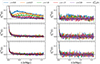 |
Fig. 1. Estimated skewness, S3(ℓ) (left panels), and kurtosis, S4(ℓ) (right panels), of the distribution of power spectrum multipoles P(ℓ)(k) in real space for the reference ΛCDM cosmology and for the five redshifts considered in this work (from top to bottom panels ℓ = 0, 2, 4). In each panel, the black line shows the prediction for a Gaussian field. |
Inspecting the left panel of Fig. 1, we can see that only the high-k part of the monopole’s skewness shows significant deviation with respect to the Gaussian field prediction. This is in good agreement with Blot et al. (2015) and with Takahashi et al. (2009). In addition, we can see that this deviation is more important at a low redshift. At z = 0 we can see the excess of skewness starting at k = 0.1 h/Mpc, while at z = 1 it starts at k = 0.2 h/Mpc, and we cannot even see it at z = 2 for the scales probed here. This behaviour is expected as the terms  ,
,  , and
, and  in Eq. (18) are becoming more important through the non-linear evolution of the matter clustering. Note that when k increases, the skewness starts to decrease again but less rapidly than in the Gaussian case; thus one could think that in the limit of an infinite number of modes the skewness is expected to vanish, which is in agreement with the central limit theorem.
Regarding the kurtosis (right panel of Fig. 1) it is more difficult to draw strong conclusions because the estimation is more affected by noise. Focusing on the monopole we can detect some excess of kurtosis around k > 0.3 h/Mpc at z = 0. However, for z > 0.5 there is no direct detection of an excess kurtosis.
In redshift space (see Fig. 2), the excess of skewness observed at high wave modes for the monopole in real space is suppressed, yielding a better agreement with the Gaussian prediction. The excess skewness of the monopole in real space appears to be transferred to the quadrupole and hexadecapole in redshift space, causing deviations from their respective predictions. Specifically, the skewness of the quadrupole decreases and becomes negative, while the skewness of the hexadecapole increases. Regarding the kurtosis, no excess can be detected at any scale, redshift, and multipole.
Since it appears that the dominant non-Gaussian contribution is the skewness, in the following we put the kurtosis aside and quantify the contribution of each term in Eq. (18) to the total skewness.
We define the relative difference of the total cumulant moments with respect to their Gaussian only contribution as
 (33)
(33)
From Eq. (11), one can show that r2, which is the non-Gaussian relative contribution to the variance, is given by
 (34)
(34)
It is directly related to the shell averaged trispectrum  .
.
Based on the structure of Eq. (18), we can write r3 as
 (35)
(35)
When considering the monopole in real space, one can show that  and
and  , which allows us to rewrite r3 as
 (36)
(36)
where
 (37)
(37)
Equation (36) highlights the fact that different terms contribute to the non-Gaussian part of ⟨X3⟩c, specifically: the bispectrun term b, the trispectrum term 3r2, and the pentaspectrum term.
We start by showing that the bispectrum contribution, b, is expected to be negligible with respect to 3r2. For this we can notice two things about the three modes k1, k2, and k3 (see Eq. (3)) defining a bispectrum configuration: first, invariance by translation imposes that −k3 = k1 + k2, and second, we need their modulus to be contained within the considered k-shell. These two constraints mean that not all triplets, k1, k2, k3, will contribute to the shell average of the bispectrum. Indeed, only pairs k1, k2 that satisfy  can contribute. Thus, only nearly equilateral configurations of the triplets will be kept in the shell averaging. We can see in Eq. (17) that there are four kinds of configurations for the bispectrum k1 + k2, k1 − k2, −k1 − k2 and k2 − k1 with respectively N1, N2, N3 and N4 number of triangular configurations which are contributing to the shell-averaged square of the bispectrum
  . As a result, defining N = N1 + N2 + N3 + N4 as the total number of triangles that contribute to the shell average and using symmetry conditions one can show that the total (i.e. double counting the repeated conjugate modes) number of triangles is roughly given by N ≃ π2 (k/kF)3. In addition, from Eq. (19) one can show that the monopole
  is related to the equilateral configuration B(k) of the bispectrum through
 (38)
(38)
In practice, when considering only half of the Fourier space (discarding non-independent modes) the four configurations of the triangles formed by k1 and k2 are not appearing with the same rate. This can be estimated directly on a Fourier grid and is represented in Fig. 3. In this figure we show that the total number N of non-degenerate triangular configurations is indeed following the expected trend. One can immediately understand that since N ∝ k3 and Nk2 ∝ k4 (see Eq. (28)) the ratio will lead to a suppression of the equilateral configuration of the bispectrum proportional to k−1. We thus expect that the term b is counting less than the trispectrum contribution, which is not suffering from this mode selection within the shell. In fact, assuming that B(k)≃P3(k) and that  (see Scoccimarro et al. 1999; Baratta et al. 2020, for a justification), one can show that we expect
 (39)
(39)
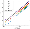 |
Fig. 3. Number of triplets, k1, k2, k3, per k-shell depending on the considered configuration, N1, N2, N3, and N4. The purple diamonds show the total number of triplets, and the black line shows the corresponding expected number. |
By estimating the second- and third-order cumulants from the ΛCDM simulation at z = 0, we can compute 3r2 and r3. In addition, we can estimate the equilateral configurations of the bispectrum B(k) on 100 000 realisations. It allows us to evaluate the contribution b to the relative excess skewness r3. In Fig. 4 we compare these three quantities. First, we can see that the overall amplitude of the bispectrum term b is indeed of the order expected from Eq. (39), which is displayed as a gray dotted line. Second, due to the suppression mechanism described above, the b contribution is more than one order of magnitude smaller than the trispectrum contribution 3r2 at the lowest accessible k and more than two orders of magnitude smaller at k = 0.2 h/Mpc. This justifies neglecting the bispectrum term b in the following sections. Thus, we are left with two terms that contribute to the relative excess of skewness r3: the trispectrum term 3r2 and the pentaspectrum term which, neglecting b, is simply r3 − 3r2.
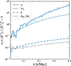 |
Fig. 4. Measurement of r3 from the ΛCDM simulation at z = 0 and its different contributions. The solid line shows the total relative difference r3, while the dashed and dot-dashed lines show the trispectrum and bispectrum contribution, 3r2 and b, respectively. The dotted black line shows a rough estimation of b based on Eq. (39). |
In Fig. 5 we show how the non-Gaussian contribution to the covariance evolves with redshift in the COVMOS realisations. In this figure 3r2 is represented in dashed line so when it crosses the level 3 (dotted line) it means that the Gaussian and the non-Gaussian part contribute the same amount to the total variance. This is confirming that when the redshift is low (z = 0), the term  starts dominating the variance already at k = 0.25 h/Mpc while at high redshift (z = 2) it happens on smaller scales (k = 0.6 h/Mpc). This is a well known result which was already shown by Takahashi et al. (2009).
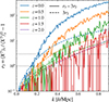 |
Fig. 5. Relative excess skewness, r3, made of two contributions: 3r2 and r3 − 3r2 (respectively in dashed and solid lines). The colours correspond to the different redshifts. For clarity of the figure, we do not show r3 − 3r2 for z = 2, as it is compatible with 0. There are two horizontal dotted black lines showing the levels 1 and 3. |
In addition, in Fig. 5 we show the contribution of the two terms r3 − 3r2 (pentaspectrum) and 3r2 (trispectrum), to r3 (excess skewness) as a function of k for the five redshifts. It appears that at low redshift the term r3 − 3r2 starts dominating already at k > 0.3 h/Mpc. However, at high redshift this term fluctuates around 0 and r3 is rather dominated by 3r2.
Based on the above observations and by expressing the ratio between the total skewness and its prediction for a Gaussian field in terms of r2 and r3 as
 (40)
(40)
we can obtain approximate expressions in the two regimes (either the pentaspectrum or the trispectrum domination regime) described above. At high redshift, when r3 is dominated by 3r2 (trispectrum domination), a simple calculation shows that when 3r2 ≃ 9 the ratio in Eq. (40) deviates from 1 by only 25%. On the other hand, when we consider low redshift and relatively non-linear scales (k > 0.3 h/Mpc) we can use the approximation
 (41)
(41)
As a result, in that regime one can approximate Eq. (40) as
 (42)
(42)
This shows that the excess of skewness is directly related to the ratio between the shell averaged pentaspectrum and the shell averaged trispectrum to the power of 3/2. As a result, Eq. (42) shows that if this ratio is not well reproduced in the COVMOS realisations we would not get a realistic excess of skewness.
Thus, one might wonder about the soundness of the COVMOS method to study the non-Gaussian behaviour of the distribution of the power spectrum estimator. To gain confidence in the COVMOS method in terms of higher-order statistics, we conducted a comparison between the COVMOSΛCDM simulation at z = 0 and a set of 12 288 N-body simulations using a comparable cosmology, the DEUS-PUR simulations (Blot et al. 2015). As demonstrated in Appendix B, our results using COVMOS exhibit a robust agreement with those obtained from N-body simulations, up to k = 0.8 h/Mpc. This comparison further validates the robustness and accuracy of the COVMOS method for analysing non-Gaussian features.
Since the skewness S3(ℓ) of the estimator of the multipoles of the power spectrum depends explicitly on higher-order correlation functions of the density field we also investigate how it changes when considering different cosmological models characterised by roughly the same power spectrum. In Fig. 6 we compare the skewness estimated in the three samples, ΛCDM, 16nu and w9p3, corresponding to three different cosmological models (see Table 1) at z = 0, both in real and redshift space. We can see that adding massive neutrinos (with 16nu) is not changing the skewness, while modifying the dark energy equation of state is only slightly affecting the large k behaviour of the real space monopole. In redshift space all multipoles skewness are unchanged by varying cosmology. It is worth noticing that all three models exhibit similar clustering amplitudes, as evidenced by their power spectra presented in Parimbelli et al. (2022).
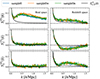 |
Fig. 6. Estimated skewness S3(ℓ) of the distribution of the power spectrum multipoles (from top to bottom panels ℓ = 0, 2, 4) P(ℓ)(k) in real (left) and redshift space (right) for the ΛCDM cosmology and its two extensions, 16nu and w9p3. In each panel the black line is the skewness expected for a Gaussian field. |
4.2. Effects of the estimator’s setting on the data distribution
In this subsection we investigate how technical details of the power spectrum estimator can impact its statistical distribution. We focus on the real-space distribution, which maximises the excess of skewness.
4.2.1. Aliasing and mass assignment scheme
Despite the soundness of the results presented above, we want to verify their robustness against changes in the choices made for the settings of the estimator. One could think of a possible dependence in the choice of the mass assignment through aliasing effects. Indeed, aliasing is introducing some correlations between modes which might induce some unexpected skewness (Baratta et al. 2020). Thus, to ensure that the observed excess of skewness in the power spectrum distribution is indeed cosmological and do not arise from any numerical artefact, we modified and compared different settings of the estimator.
We tested three different settings. The first was (i) the interlacing technique (Sefusatti et al. 2016), in which one can choose to reduce aliasing arising when using fast Fourier transforms. The second concerned (ii) the type of mass assignment scheme used to interpolate the particles over the grid before estimating the power spectrum, where we tested two of them: the cloud-in-cell and piecewise cubic spline. The third involved (iii) the precision of the grid, where we chose a standard mesh of Nmesh = 512 points per dimension and a less precise one with Nmesh = 128.
The results are shown in Fig. 7. They clearly demonstrate that, regardless of the choice of these three settings, the skewness of the power spectrum distribution remains the same, including when close to the Nyquist mode kNyNmesh = πNmesh/L. This indicates that the type of estimator used does not affect the skewness of the power spectrum.
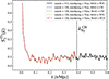 |
Fig. 7. Estimated skewness of the power spectrum monopole in real space for different estimator settings on a reduced set of 10 000 realisations. |
4.2.2. Fourier mode binning
In galaxy survey analyses, it is common to adapt the power spectrum wave-mode bin width Δk to accurately capture the cosmological information across various scales. The goal is to find the optimal Δk to balance the need for detailed understanding of the power spectrum behaviour across scales while minimising the noise, the correlations between different bins and the number of bins in the data-vector. For example it is possible to enlarge the binning in k such that one can reduce the size of the data-vector. This is particularly useful to obtain cosmological constraints based on a covariance matrix which is estimated from a finite set of realisations (Gouyou Beauchamps et al. 2025).
We thus want to observe the effect of the bin width on the skewness of the estimator of the power spectrum distribution in light of the analytical formalism presented in Sect. 2. Indeed, we expect that enlarging the bin width will affect the shell averaged poly-spectra entering in the third-order cumulant of the distribution of the power spectrum estimator (see Eq. (18)). In the limit of a Gaussian density field, where the skewness is given by Eq. (26), the only effect we can expect is that, by increasing the size of the bins, the number of modes within the Fourier shell will also increase, resulting in a decrease of the skewness. However, considering a non-Gaussian density field it is difficult to predict the effect of the binning with simple arguments. As a result, in this section we systematically test the effect of increasing the bin width of the estimated monopole power spectrum in real space.
Figure 8 displays the excess skewness of the power spectrum distribution with respect to the Gaussian field prediction, at z = 0 and in real space, for various bin widths, ranging from Δk = kF = 0.006 h/Mpc to Δk = 0.1 h/Mpc. We can see that increasing the bin width produces more excess skewness, especially on intermediate scales, between k = 0.15 and 0.4 h/Mpc. In that range we can see that the excess skewness can increase by 66% going from the reference binning size (i.e. the fundamental frequency) to largest one. On these scales higher-order statistics, and thus the non-Gaussian terms in Eq. (18), start to be relevant. On the contrary, for k > 0.55 h/Mpc the increase with the binning size is less than 15%. Since in this regime the skewness can be approximated with Eq. (42), it means that the ratio between the pentaspectrum and trispectrum to the power 3/2 is close to be constant when increasing the shell size.
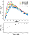 |
Fig. 8. Impact of wave mode binning. Top: Difference between the estimated skewness and the Gaussian field prediction for the real-space power spectrum at z = 0 for different bin sizes, Δk. Bottom: Skewness at k = 0.3 h/Mpc with respect to Δk. |
In the lower panel of Fig. 8 we can appreciate how the skewness is increasing with the binning size at fixed k = 0.3 h/Mpc. It appears that it saturates at around 7 times the fundamental frequency. In conclusion, even a drastic increase in the binning size does not increase the skewness of the estimator of the power spectrum more than 50%.
4.3. Effects of survey-related features on the data distribution
In this subsection, we investigate the impact of characteristic features of a survey on the statistical distribution of the power spectrum estimator. Since we have shown in Sect. 4 that being in real space maximises the excess of skewness we keep the same setting in the following.
4.3.1. Sample density
First, we examine the effect of the number density of objects in the catalogue. Indeed, since shot noise affects all N-point correlation functions, it should induce a non-zero trispectrum and pentaspectrum and can thus modulate the expected skewness when the Gaussian contribution is sub-dominant. Our reference catalogue, ΛCDM at z = 0, has a number density ρ = 0.1 (h/Mpc)3. We generated a set of three sparser catalogues with densities of ρ = 0.05, 0.01, and 0.001 (h/Mpc)3 and for each of them we estimate the skewness of the real-space monopole power spectrum.
The top panel of Fig. 9 displays the average power spectrum of the reference sample, as well as the shot noise amplitude of the other samples. The middle panel shows the estimated skewness S3(0)(k) in all samples. From this figure, it is evident that increasing the shot noise level tends to lower the excess skewness. The suppression starts to be effective at the wave mode for which the power spectrum and the shot noise level have the same amplitude. One can notice that when shot noise dominates completely over the signal, no excess skewness becomes detectable. This is in agreement with the expectation. In fact, when the signal is dominated by shot noise we expect the power spectrum to be equal to PSN = 1/ρ. In addition, the higher-order N-point spectra such as the bispectrum, trispectrum, and pentaspectrum are affected in a non-trivial way by the shot noise (see Blot et al. 2015, for the explicit expressions up to the trispectrum). However, it is fairly intuitive that a pure Poisson distribution will be characterised by  ,
,  and
and  . Thus, at high k we expect ⟨X2⟩c ≃ kF3PSN3 and ⟨X3⟩c ≃ kF6PSN5, from which it follows that
 (43)
(43)
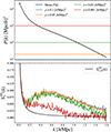 |
Fig. 9. Impact of the shot noise. Top: Mean power spectrum for the reference sample and the different level of shot noise corresponding to each density. Bottom: Estimated skewness for the different densities considered (coloured lines) and the Gaussian field prediction (black line). |
when the signal is dominated by shot noise. The Eq. (43) suggests that the skewness should increase with the shot-noise power spectrum PSN which seems contrary to what is observed in Fig. 9. However, considering the most extreme shot-noise case (ρ = 0.001 (h/Mpc)3) we expect the skewness to decrease to a value of 0.016 at large k, which is a level too low to be detected in our case. The fact that the shot noise reduces the skewness was also observed in Lin et al. (2020) in the case of weak lensing two-point correlation functions.
In Euclid Collaboration: Mellier et al. (2025) it is predicted that the total spectroscopic sample of Euclid will have a density of less than ρ = 10−3 (h/Mpc)3, which is comparable to the highest level of shot noise shown in Fig. 9.
4.3.2. Survey window function
As observed in Upham et al. (2021), another observational aspect that can significantly impact the distribution of two-point statistics is the survey mask. In order to investigate this effect, we carve two arbitrary cone-like geometries within the periodic boxes generated with COVMOS. We define two different cones that both have an aperture of semi-angle θ = π/9. The big cone has a radial extension of [rmin,rmax] = [600, 1400] Mpc/h and the small one [rmin,rmax] = [800, 1000] Mpc/h. The big and small cones have respectively a volume of 0.3 (Gpc/h)3 and 0.06 (Gpc/h)3. The particle number density is the same as the reference value of ρ = 0.1 (h/Mpc)3 that we considered for the periodic box. In Fig. 10 we show how the small and big cones are compared with the reference comoving box.
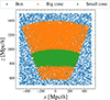 |
Fig. 10. Two-dimensional projection of a sample of particles from the three different geometries considered: the periodic box and the big and small cone. |
We estimate the power spectrum in each of the 100 000 realisations at z = 0, in real space, for both cone-like geometries with an enclosing box of sised 1000 h−1 Mpc. As we are no longer analysing a periodic box we need to take care about the effect of the mask in the estimation of the power spectrum (see Beutler et al. 2017 or GB-2025 for more details). To have an accurate estimation of the survey mask power spectrum we take the average power spectrum from 50 realisations of a uniform random distribution following the cone geometries with 20 times the reference density.
From the distribution of the measured power spectra we can estimate the skewness of its distribution (Eq. (23)) in the small and big cones and compare them to the reference periodic box. In addition, we compare these to the Gaussian field prediction. However, if in the case of a periodic box it is fairly straightforward to get this prediction (see Appendix A), in the case of a masked field calculations become significantly more complicated. We need to be careful about the effect of the integral constraint (IC, de Mattia & Ruhlmann-Kleider 2019), which is expected to propagate into the skewness.
The IC comes from the fact that the density contrast is defined from the mean number density of objects in a given catalogue. However, we can only estimate it from the same volume that we have at our disposal to estimate two-point statistics. This gives rise to correlation between large- and short-scale modes. Thus, in order to properly compare the skewness estimated in the COVMOS realisations with respect to the Gaussian field case, we generate NG = 100 000 realisations of masked Gaussian fields with and without taking into account the IC. We set-up these Gaussian fields, dubbed ν(x) in the following, such that they have the same power spectrum as the COVMOS realisations.
In the following we explain how we include or not the contribution from IC in these Gaussian realisations. As explained above, the mean number density  that we estimate inside a given mask of volume V, as
  , is different from the true number density n0 = ρ. Thus, within the same volume V the estimated density contrast δIC(x) is different from the true one δ(x). The relation between the two can be obtained by noticing that the only quantity which is conserved is the local number density n(x), implying that
![Mathematical equation: $$ \begin{aligned} \bar{n} \left[ 1 + \delta _{\rm IC}(\boldsymbol{x}) \right] = n_0 \left[ 1 + \delta (\boldsymbol{x}) \right]. \end{aligned} $$](/articles/aa/full_html/2026/04/aa56642-25/aa56642-25-eq76.gif) (44)
(44)
Due to the finite size of the geometry,  fluctuates from one realisation to another such that
  , where
 (45)
(45)
As a result, one can relate the Gaussian field ν(x) to the corresponding Gaussian field νIC(x) affected by the IC directly with
 (46)
(46)
We can thus efficiently estimate the skewness of the power spectrum estimated in the Gaussian realisations with and without the presence of the IC. We found that without the IC, one can find an empirical model for the skewness of a Gaussian field in the cone geometries. Indeed, by defining an effective fundamental mode for a given geometry of volume V as kF, eff := 2π/V1/3, one can define an effective number of independent modes in a given k-shell as Neff := 2π k2/kF, eff2. Empirically we found that  provides a good fit for both volumes we consider.
In Fig. 11 we show the skewness estimated from the COVMOS realisations for the two cones and the periodic box and compare them to the skewness estimated from the Gaussian realisations described above. We can see that the presence of a mask increases the level of skewness at all scales. The smaller is the mask the larger is the increase of the skewness level. This is expected because the application of the mask on the density field correlates Fourier modes. Indeed, this is in a way similar to increasing the size of the k-shell (see Sect. 4.2.2).
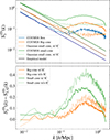 |
Fig. 11. Impact of the survey mask. Top: Estimated skewness in the three geometries from the COVMOS simulations (light coloured plain lines) and the Gaussian field realisations, where the contribution from IC is not subtracted (dotted lines). We also show our empirical model for the Gaussian field without the IC contribution (dark coloured solid lines). Bottom: Difference between the skewness estimated in the COVMOS simulations and the Gaussian realisations with and without IC (light coloured plain and dotted lines, respectively). |
Our empirical model, which reproduces the skewness obtained from a Gaussian field without IC is shown in the top panel of Fig. 11 with dark solid lines. Comparing this empirical model, which does not include the effect of IC, to the skewness estimated from the Gaussian field with IC (dark solid lines against dotted lines in the top panel of Fig. 11), we observe that on small scales the IC itself is introducing an excess of skewness in the distribution of the power spectrum. We notice that its amount depends on the volume used to estimate the mean number density and that it is roughly constant at large k.
As a result, to quantify the excess skewness with respect to the Gaussian case, one needs to subtract the Gaussian skewness with IC to the estimated skewness in the COVMOS catalogues. This is shown in the lower panel of Fig. 11, where it appears clearly that when the considered volume is small (0.06 [Gpc/h]3) it is important to take into account the skewness induced by the IC while when the volume is larger (0.3 [Gpc/h]3) the absolute contribution from the IC to the total excess skewness becomes subdominant. As a reference, the smallest redshift bin for the Euclid spectroscopic sample of the first data release (DR1) is expected to be around 1.5 (Gpc/h)3, thus the IC should not increase the level of skewness in the Euclid two-point summary statistics in Fourier space.
5. Statistical distribution of individual Fourier modes within a shell
Up to now we studied the distribution of the shell-averaged estimated power spectrum and found that the excess of skewness with respect to a Gaussian distribution originates from the shell-averaged higher-order statistics, such as the trispectrum and pentaspectrum. We now want to understand the origin of this non-Gaussian distribution and whether it is generated by an intrinsic non-Gaussian distribution of each individual Fourier mode. In this section, we are thus interested in the distribution of square modulus of the density contrast Xi := |δki|2 evaluated at each individual wave mode within a shell k.
As shown in Appendix A, when δk is a Gaussian field then Xi is expected to follow an exponential distribution. We thus, want to understand whether the skewness in the shell averaging process is generated by an intrinsic departure from the expected exponential distribution of each individual Xi or from the correlations between them. To achieve this we focus on the distribution of a sub-sample of modes within four Fourier shells k = 0.2 h/Mpc, k = 0.3 h/Mpc, k = 0.4 h/Mpc, and k = 0.5 h/Mpc. In each k-shell, we randomly select 1000 square modulus Xi, for which we can compute the one-point cumulant moments up to an order of five. We can compare these cumulant moments to the predicted ones assuming an exponential distribution (i.e. in the case of a Gaussian field). The latter can be expressed as
 (47)
(47)
as shown in Appendix A.
In Fig. 12 we display the relative deviation between the estimated cumulant moments of Xi with respect to their prediction of Eq. (47). Since for each shell we have 1000 square modulus Xi we only show the mean relative deviation (computed over the 1000 modes) and the corresponding dispersion over the considered shell. We can see a very good agreement between the estimation and its prediction in the case of an exponential distribution.
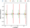 |
Fig. 12. Relative difference between the cumulants (up to an order of five) of each individual mode and their predictions in the case of a Gaussian field (see Eq. (47)). The error bars show the dispersion obtained for the 1000 considered wave modes. |
Despite the fact that the first five cumulant moments are well reproduced when fixing the first moment to the expectation value evaluated over the 100 000 realisations, one could argue that this does not prove that the full distribution is well represented by an exponential distribution. Thus, we conducted a Kolmogorov–Smirnof (KS) test to compare each distribution of the 4 × 1000 wave modes with an exponential distribution. For each of the 4 × 1000 wave modes, we generate a set 100 000 values extracted from an exponential distribution with the estimated mean value and we perform the KS test to compare the true distribution and the exponential one. It turns out that the lowest probability assessing the inconsistency between the observed and expected distribution over all the tested modes is 0.73. It means that for none of the 4000 modes at our disposal we can reject the hypothesis that the distribution is exponential without having a very high probability of drawing a wrong conclusion. Thus, it appears that the square modulus at each measured wave mode is following with a great accuracy an exponential distribution.
In conclusion, this means that despite the fact that the density field is non-Gaussian, the distribution of the square modulus of the Fourier space density field is following the distribution which would be expected if the field were Gaussian. This is a clear indication that the main source of the excess skewness of the power spectrum distribution is due to the correlation between wave modes.
6. Conclusions
Given the level of precision of the cosmological constraints the Euclid mission aims at providing, the reliability of common assumptions that are usually made on the likelihood function must be checked to the same level of precision. One crucial assumption that was studied in detail in this paper is to consider that two-point statistics follow a Gaussian distribution.
We could test this assumption and compare it to our theoretical expectations with great precision thanks to the COVMOS method, which has been proven to be suitable to study the covariance matrices of two-point statistics (Baratta et al. 2020, 2023; Gouyou Beauchamps et al. 2025) and the N-point distribution of two-point statistics in the present work (see the comparison with the DEUS-PUR simulations in Appendix B).
We first derived the analytical expressions of the second- and third-order cumulants of the power spectrum distribution in terms of the N-point functions of the density field. This allowed us to directly put in evidence of the relation between the non-Gaussianity of the density field and the non-Gaussianity of the power spectrum distribution and isolate the competing terms contributing to this distribution (see Eqs. (11) and (18)). In order to understand which terms were dominating depending on the scales, we derived the analytical expressions of the skewness and kurtosis of the multipoles of the power spectrum in both real and redshift space assuming a Gaussian field (see Eqs. (26)–(32) and Appendix A).
To compare these approximate predictions to their equivalent estimations for a more realistic non-Gaussian field, we generated several simulation samples, each containing 100 000 COVMOS realisations of the matter density field, while varying the redshift and the cosmological model both in real and redshift space. This allowed us to estimate the skewness and kurtosis of the distribution of the power spectrum monopole in real space and confirm, as was already observed in Takahashi et al. (2009) and Blot et al. (2015), the presence of an excess of skewness on non-linear scales (k > 0.1 h/Mpc at z = 0). In addition, for the first time, we also estimated the skewness and kurtosis of the power spectrum multipoles in redshift space. We observed that the presence of RSD transfers the excess skewness of the monopole in real space to the multipoles but significantly reduces its overall amplitude (by roughly a factor of ten).
Based on our predictions and the estimation of the skewness in the COVMOS samples, we could demonstrate that the bispectrum contribution to the skewness (see Eq. (37)) is negligible because only a small fraction of the triangular configurations contribute to ⟨X3⟩c. This led us to understand that on intermediate scales, the excess skewness is dominated by the trispectrum contribution, while on small scales it is dominated by the pentaspectrum of the matter density field.
We also extended this study to other cosmological models, including massive neutrinos and a time-varying dark energy equation of state. We have shown that varying the cosmological model does not have a significant impact on the skewness.
We then varied different settings in the estimation of the power spectrum to gauge their effects on its skewness. We observed that the aliasing due to the use of fast Fourier transforms has no impact on the skewness. However, varying the size of the k-shells of the power spectrum has a significant impact on the skewness, as increasing their size produces an increase in the excess skewness of up to 20%.
We also explored how the skewness was impacted by the number density of objects, which is a feature that is specific to a given survey. We saw that increasing the level of shot noise has the effect of reducing the skewness of the power spectrum on scales where the power spectrum is dominated by the shot noise. For a level of shot noise similar to the one expected for the Euclid spectroscopic sample, the skewness is greatly reduced (by around 50% for k ∼ 0.4 h/Mpc, which are the most impacted scales).
However, all of this was done while assuming a periodic universe in a box, which is far from the reality of the data that will be obtained with Euclid (or any other survey). Indeed, we found that restricting the density field to a cone-shaped survey mask significantly increases the skewness of the power spectrum in two different ways. Firstly, reducing the surveyed volume necessarily reduces the number of available Fourier modes, but it also correlates them, thus increasing the level of skewness at all scales. Secondly, the presence of the IC has a specific impact on the excess skewness on small scales, increasing it for smaller volumes.
Finally, in an attempt to understand the origin of the skewness of the power spectrum, we looked at the statistical distribution of each individual wave mode,  . We found, with a high level of accuracy, that they conserve an exponential distribution (θ−1 e−X/θ, with parameter
  ) no matter their configurations. This led us to conclude that the extra skewness observed on small scales appears because of the correlation between wave modes within a k-shell.
To conclude, it is clear from this work that the distribution of two-point statistics is not Gaussian, and we understand the reasons for that. In particular, the shot noise, the scale binning, and the survey mask are factors that can significantly enhance its skewness. However, it is still unclear whether the assumption of a Gaussian likelihood, given non-Gaussian distributed data, would bias parameter inference for a dataset similar to what will be obtained with Euclid. This is explored in our companion paper GB-2025, where we show that these non-Gaussian features do not introduce a significant bias in cosmological parameter estimation for Euclid-like datasets.
Acknowledgments
The Euclid Consortium acknowledges the European Space Agency and a number of agencies and institutes that have supported the development of Euclid, in particular the Agenzia Spaziale Italiana, the Austrian Forschungsförderungsgesellschaft funded through BMK, the Belgian Science Policy, the Canadian Euclid Consortium, the Deutsches Zentrum für Luft- und Raumfahrt, the DTU Space and the Niels Bohr Institute in Denmark, the French Centre National d’Etudes Spatiales, the Fundação para a Ciência e a Tecnologia, the Hungarian Academy of Sciences, the Ministerio de Ciencia, Innovación y Universidades, the National Aeronautics and Space Administration, the National Astronomical Observatory of Japan, the Netherlandse Onderzoekschool Voor Astronomie, the Norwegian Space Agency, the Research Council of Finland, the Romanian Space Agency, the State Secretariat for Education, Research, and Innovation (SERI) at the Swiss Space Office (SSO), and the United Kingdom Space Agency. A complete and detailed list is available on the Euclid web site (www.euclid-ec.org). The project leading to this publication has received funding from Excellence Initiative of Aix-Marseille University -A*MIDEX, a French “Investissements d’Avenir” programme (AMX-19-IET-008 -IPhU). The DEMNUni-cov simulations were carried out in the framework of “The Dark Energy and Massive Neutrino Universe covariances” project, using the Tier-0 Intel OmniPath Cluster Marconi-A1 of the Centro Interuniversitario del Nord-Est per il Calcolo Elettronico (CINECA). We acknowledge a generous CPU and storage allocation by the Italian Super-Computing Resource Allocation (ISCRA) as well as from the coordination of the “Accordo Quadro MoU per lo svolgimento di attività congiunta di ricerca Nuove frontiere in Astrofisica: HPC e Data Exploration di nuova generazione”, together with storage from INFN-CNAF and INAF-IA2.
References
- Abbott, T. M. C., Aguena, M., Alarcon, A., et al. 2022, Phys. Rev. D, 105, 023520 [CrossRef] [Google Scholar]
- Agrawal, A., Makiya, R., Chiang, C.-T., et al. 2017, JCAP, 10, 003 [CrossRef] [Google Scholar]
- Alonso, D., Ferreira, P. G., & Santos, M. G. 2014, MNRAS, 444, 3183 [NASA ADS] [CrossRef] [Google Scholar]
- Asgari, M., Lin, C.-A., Joachimi, B., et al. 2021, A&A, 645, A104 [NASA ADS] [CrossRef] [EDP Sciences] [Google Scholar]
- Baratta, P., Bel, J., Plaszczynski, S., & Ealet, A. 2020, A&A, 633, A26 [NASA ADS] [CrossRef] [EDP Sciences] [Google Scholar]
- Baratta, P., Bel, J., Gouyou Beauchamps, S., & Carbone, C. 2023, A&A, 673, A1 [NASA ADS] [CrossRef] [EDP Sciences] [Google Scholar]
- Bautista, J. E., Paviot, R., Vargas Magaña, M., et al. 2021, MNRAS, 500, 736 [Google Scholar]
- Beutler, F., Seo, H.-J., Saito, S., et al. 2017, MNRAS, 466, 2242 [Google Scholar]
- Blot, L., Corasaniti, P. S., Alimi, J. M., Reverdy, V., & Rasera, Y. 2015, MNRAS, 446, 1756 [NASA ADS] [CrossRef] [Google Scholar]
- Carbone, C., Petkova, M., & Dolag, K. 2016, JCAP, 7, 034 [CrossRef] [Google Scholar]
- Chevallier, M., & Polarski, D. 2001, Int. J. Mod. Phys. D, 10, 213 [Google Scholar]
- de Mattia, A., & Ruhlmann-Kleider, V. 2019, JCAP, 8, 036 [Google Scholar]
- DESI Collaboration (Aghamousa, A., et al.) 2016, ArXiv e-prints [arXiv:1611.00036] [Google Scholar]
- DESI Collaboration (Adame, A. G., et al.) 2025, JCAP, 2025, 012 [Google Scholar]
- Euclid Collaboration (Mellier, Y., et al.) 2025, A&A, 697, A1 [Google Scholar]
- Fisher, K. B., Davis, M., Strauss, M. A., Yahil, A., & Huchra, J. P. 1993, ApJ, 402, 42 [Google Scholar]
- Gil-Marín, H., Bautista, J. E., Paviot, R., et al. 2020, MNRAS, 498, 2492 [Google Scholar]
- Gouyou Beauchamps, S., Baratta, P., Escoffier, S., et al. 2025, A&A, 693, A226 [NASA ADS] [CrossRef] [EDP Sciences] [Google Scholar]
- Hall, A., & Taylor, A. 2022, Phys. Rev. D, 105, 123527 [NASA ADS] [CrossRef] [Google Scholar]
- Hamimeche, S., & Lewis, A. 2008, Phys. Rev. D, 77, 103013 [NASA ADS] [CrossRef] [Google Scholar]
- Hand, N., Feng, Y., Beutler, F., et al. 2018, AJ, 156, 160 [Google Scholar]
- Ivezić, Ž., Kahn, S. M., Tyson, J. A., et al. 2019, ApJ, 873, 111 [Google Scholar]
- Lin, C.-H., Harnois-Déraps, J., Eifler, T., et al. 2020, MNRAS, 499, 2977 [NASA ADS] [CrossRef] [Google Scholar]
- Linder, E. V. 2003, Phys. Rev. Lett., 90, 091301 [Google Scholar]
- Meiksin, A., & White, M. 1999, MNRAS, 308, 1179 [NASA ADS] [CrossRef] [Google Scholar]
- More, S., Sugiyama, S., Miyatake, H., et al. 2023, Phys. Rev. D, 108, 123520 [NASA ADS] [CrossRef] [Google Scholar]
- Parimbelli, G., Anselmi, S., Viel, M., et al. 2021, JCAP, 1, 009 [NASA ADS] [Google Scholar]
- Parimbelli, G., Carbone, C., Bel, J., et al. 2022, JCAP, 11, 041 [Google Scholar]
- Percival, W. J., Friedrich, O., Sellentin, E., & Heavens, A. 2022, MNRAS, 510, 3207 [NASA ADS] [CrossRef] [Google Scholar]
- Planck Collaboration VI. 2020, A&A, 641, A6 [NASA ADS] [CrossRef] [EDP Sciences] [Google Scholar]
- Planck Collaboration XVI. 2014, A&A, 571, A16 [NASA ADS] [CrossRef] [EDP Sciences] [Google Scholar]
- Scoccimarro, R., Zaldarriaga, M., & Hui, L. 1999, ApJ, 527, 1 [NASA ADS] [CrossRef] [Google Scholar]
- Sefusatti, E., Crocce, M., Scoccimarro, R., & Couchman, H. 2016, MNRAS, 460, 3624 [NASA ADS] [CrossRef] [Google Scholar]
- Sellentin, E., & Heavens, A. F. 2016, MNRAS, 456, L132 [Google Scholar]
- Smith, R. E. 2009, MNRAS, 400, 851 [NASA ADS] [CrossRef] [Google Scholar]
- Smith, R. E., & Marian, L. 2015, MNRAS, 454, 1266 [Google Scholar]
- Takahashi, R., Yoshida, N., Takada, M., et al. 2009, ApJ, 700, 479 [NASA ADS] [CrossRef] [Google Scholar]
- Upham, R. E., Brown, M. L., & Whittaker, L. 2021, MNRAS, 503, 1999 [NASA ADS] [CrossRef] [Google Scholar]
- Xavier, H. S., Abdalla, F. B., & Joachimi, B. 2016, MNRAS, 459, 3693 [NASA ADS] [CrossRef] [Google Scholar]
We use the following Fourier convention 
Note that this is an abuse of notation because S3(ℓ) is not actually a multipole of the Legendre expansion as P(ℓ)(k).
Appendix A: Skewness and kurtosis for the multipoles
In this appendix, we derive the expressions of the estimation of the skewness S3(ℓ) and kurtosis S4(ℓ) of the estimator of the power spectrum multipoles. We define the estimator X as a shell average at a fixed k modulus as
 (A.1)
(A.1)
where the sum runs over all modes contained in a given shell and μi is the cosine of the angle between the wave vector k and the line-of-sight (along the z direction of the periodic box). Defining the variable  and the coefficients
  , one can express the estimator as a weighted average over the random variable Xi,
 (A.2)
(A.2)
Since the variable Xi is made of the sum of the square of the real and imaginary part of the Fourier modes  , then it means that it follows an exponential distribution 𝒫 (Fisher et al. 1993) of parameter
  , and thus
 (A.3)
(A.3)
Its associated moment generating function  is therefore given by
 (A.4)
(A.4)
and the moment generating function of Yi := Xiai(ℓ) is given by  . Since we assume that each Xi variable is independent from each other, the same property holds for the Yi variable, thus one can express the joint Nk-point moment generating function of the Nk variables as
 (A.5)
(A.5)
Thanks to the properties of the moment generating function, one can express the moment generating function of the sum of Yi which is the variable X as  and its corresponding cumulant generating function
  as
as
 (A.6)
(A.6)
One can take the n-th derivative of the above expression to obtain
 (A.7)
(A.7)
from which it is straight forward to express the n-th order cumulant moments  as
as
 (A.8)
(A.8)
Since the skewness S3 and kurtosis S4 are defined as
 (A.9)
(A.9)
we need to evaluate expression (A.8) for n = 2, 3, 4. Under some further hypothesis, one can obtain a closed analytical form. Assuming that the discrete sum over the shell can be approximated with its continuous limit, it follows that
 (A.10)
The above equation can be approximated when assuming that we are in real space, thus the power spectrum depends only on the modulus k of the wave vector k:
 (A.11)
which is the usual expression for the variance of the power spectrum multipole estimator. For the third-order cumulant moment, we get
 (A.12)
where we see the Wigner 3-j symbols, and finally for the fourth order,
 (A.13)
This allowed us to express the skewness and kurtosis in the case of a Gaussian field as
 (A.14)
and
 (A.15)
Appendix B: Validation of the COVMOS method against the DEUS-PURN-body simulations
Here, we compare the results from the COVMOS realisations to those from the DEUS-PURN-body simulation suite. The latter consists of 12 288 simulations with a volume of 656 (Mpc/h)3 containing 2563 tracer particles. All simulations have a ΛCDM cosmology characterised by the following set of parameter values (h, Ωmh2, Ωbh2, ns, σ8) = (0.72, 0.1334, 0.02258, 0.963, 0.801). Using these simulations, Blot et al. (2015) have estimated the skewness of the monopole power spectrum estimator. We use their estimates to validate the skewness of the power spectrum we have obtained from the ΛCDM COVMOS realisations at z = 0, 0.5, 1 and 1.5. It is important to remark that the DEUS-PUR estimates have been obtained with a binning in k that is set to half the fundamental frequency of the DEUS-PUR simulation box. Thus, for a given value of k, the number of independent modes may differ from the COVMOS case.
In Fig. B.1 we show the estimated skewness  at z = 0, 0.5, 1, and 1.5 from the COVMOS samples and from DEUS-PUR. We also show the Gaussian predictions for each case and the corresponding ratios, which exhibit the excess of non-Gaussianity due to the non-linearity of the matter density field. In plotting the excess non-Gaussianity of the COVMOS sample we have rescaled the ratio by a factor of
  , as we explain later in the text.
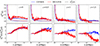 |
Fig. B.1. Comparison between COVMOS and DEUS-PUR. Top: Skewness of the distribution of the monopole of the real-space matter power spectrum (COVMOS and DEUS-PUR) in solid blue and red lines. The dashed line represents the corresponding predictions in the case of a Gaussian density field, computed using Eq. (26). Bottom: Ratio of the estimated skewness to the Gaussian field prediction, following the same colour code. |
First of all, we can see that for each case the estimated skewness follows the Gaussian density field prediction on large scales. At z = 0 this occurs up to k = 0.2 h/Mpc and extends up to k = 0.5 h/Mpc at z = 1.5. At smaller scales, we can see an excess of non-Gaussianity due to the on-set of non-linearities that propagates from small to large scales for decreasing redshifts. It is worth noticing that in the case of the DEUS-PUR results, the estimated skewness drops at large k, with a greater effect at large redshifts. A similar trend can also be seen in the case of the COVMOS sample, though with a significant smaller amplitude. This is a numerical simulation resolution effect. In the case of the DEUS-PUR simulations, the effect is mitigated at smaller redshifts, where the resolution of the force calculation at small scales is improved by the adaptive-mesh refinement scheme. Indeed, if we conservatively consider only modes corresponding to scales larger than twice the coarse cell of the DEUS-PUR simulations, k ≲ kNy/2 = 0.6 h/Mpc, we are granted that the estimate skewness is free of such numerical systematic errors. The COVMOS samples, on the other hand, have been generated using power spectra estimated from the DEMNUni-Cov simulations that have greater spatial and mass resolution than the DEUS-PUR runs with a Nyquist frequency kNy = 3 h/Mpc. That is why such an effect is much smaller than in the case of the DEUS-PUR estimates.
Yet, before comparing the excess non-Gaussianity of the COVMOS samples to that from DEUS-PUR, we should consider the effect of the different binning in k and different volume of the simulations. For this, we can use the approximation of the ratio of the excess skewness given by Eq. (42) since we are looking at non-linear scales (k ≳ 0.2 h/Mpc at z = 0). Indeed, given a binning Δk, we have that Nk ≃ 2π k2 Δk/kF3, thus Eq. (42) reads as
 (B.1)
(B.1)
This shows that the simulation volume does not affect that excess skewness, only the binning in k. Given that the binning adopted for the COVMOS samples is twice as large as that of DEUS-PUR, the corresponding excess skewness differs by a factor of  . In the bottom panels of Fig. B.1, we have shown the excess skewness of the COVMOS samples rescaled by a factor of
  which agrees well with the estimates from DEUS-PUR over the range of non-linear scales which are unaffected by resolution effects. This validates the COVMOS analysis and demonstrates that such synthetic samples are able to reproduce the correct level of excess skewness expected from full N-body simulations.
All Tables
Redshift at which the COVMOS mock catalogue samples considered in this work have been generated.
All Figures
|
Fig. 1. Estimated skewness, S3(ℓ) (left panels), and kurtosis, S4(ℓ) (right panels), of the distribution of power spectrum multipoles P(ℓ)(k) in real space for the reference ΛCDM cosmology and for the five redshifts considered in this work (from top to bottom panels ℓ = 0, 2, 4). In each panel, the black line shows the prediction for a Gaussian field. |
| In the text | |
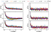 |
Fig. 2. Same as Fig. 1 but in redshift space. |
| In the text | |
|
Fig. 3. Number of triplets, k1, k2, k3, per k-shell depending on the considered configuration, N1, N2, N3, and N4. The purple diamonds show the total number of triplets, and the black line shows the corresponding expected number. |
| In the text | |
|
Fig. 4. Measurement of r3 from the ΛCDM simulation at z = 0 and its different contributions. The solid line shows the total relative difference r3, while the dashed and dot-dashed lines show the trispectrum and bispectrum contribution, 3r2 and b, respectively. The dotted black line shows a rough estimation of b based on Eq. (39). |
| In the text | |
|
Fig. 5. Relative excess skewness, r3, made of two contributions: 3r2 and r3 − 3r2 (respectively in dashed and solid lines). The colours correspond to the different redshifts. For clarity of the figure, we do not show r3 − 3r2 for z = 2, as it is compatible with 0. There are two horizontal dotted black lines showing the levels 1 and 3. |
| In the text | |
|
Fig. 6. Estimated skewness S3(ℓ) of the distribution of the power spectrum multipoles (from top to bottom panels ℓ = 0, 2, 4) P(ℓ)(k) in real (left) and redshift space (right) for the ΛCDM cosmology and its two extensions, 16nu and w9p3. In each panel the black line is the skewness expected for a Gaussian field. |
| In the text | |
|
Fig. 7. Estimated skewness of the power spectrum monopole in real space for different estimator settings on a reduced set of 10 000 realisations. |
| In the text | |
|
Fig. 8. Impact of wave mode binning. Top: Difference between the estimated skewness and the Gaussian field prediction for the real-space power spectrum at z = 0 for different bin sizes, Δk. Bottom: Skewness at k = 0.3 h/Mpc with respect to Δk. |
| In the text | |
|
Fig. 9. Impact of the shot noise. Top: Mean power spectrum for the reference sample and the different level of shot noise corresponding to each density. Bottom: Estimated skewness for the different densities considered (coloured lines) and the Gaussian field prediction (black line). |
| In the text | |
|
Fig. 10. Two-dimensional projection of a sample of particles from the three different geometries considered: the periodic box and the big and small cone. |
| In the text | |
|
Fig. 11. Impact of the survey mask. Top: Estimated skewness in the three geometries from the COVMOS simulations (light coloured plain lines) and the Gaussian field realisations, where the contribution from IC is not subtracted (dotted lines). We also show our empirical model for the Gaussian field without the IC contribution (dark coloured solid lines). Bottom: Difference between the skewness estimated in the COVMOS simulations and the Gaussian realisations with and without IC (light coloured plain and dotted lines, respectively). |
| In the text | |
|
Fig. 12. Relative difference between the cumulants (up to an order of five) of each individual mode and their predictions in the case of a Gaussian field (see Eq. (47)). The error bars show the dispersion obtained for the 1000 considered wave modes. |
| In the text | |
|
Fig. B.1. Comparison between COVMOS and DEUS-PUR. Top: Skewness of the distribution of the monopole of the real-space matter power spectrum (COVMOS and DEUS-PUR) in solid blue and red lines. The dashed line represents the corresponding predictions in the case of a Gaussian density field, computed using Eq. (26). Bottom: Ratio of the estimated skewness to the Gaussian field prediction, following the same colour code. |
| In the text | |
Current usage metrics show cumulative count of Article Views (full-text article views including HTML views, PDF and ePub downloads, according to the available data) and Abstracts Views on Vision4Press platform.
Data correspond to usage on the plateform after 2015. The current usage metrics is available 48-96 hours after online publication and is updated daily on week days.
Initial download of the metrics may take a while.