| Issue |
A&A
Volume 708, April 2026
|
|
|---|---|---|
| Article Number | A97 | |
| Number of page(s) | 13 | |
| Section | The Sun and the Heliosphere | |
| DOI | https://doi.org/10.1051/0004-6361/202556974 | |
| Published online | 01 April 2026 | |
Observational insights into Sr I 4607 Å scattering polarization with DKIST/ViSP
1
Istituto ricerche solari Aldo e Cele Daccò (IRSOL), Faculty of Informatics, Università della Svizzera italiana, 6605 Locarno, Switzerland
2
Instituto de Astrofísica de Canarias, 38205 La Laguna, Tenerife, Spain
3
Departamento de Astrofísica, Facultad de Física, Universidad de La Laguna, 38206 La Laguna, Tenerife, Spain
4
Euler Institute, Faculty of Informatics, Università della Svizzera italiana, 6900 Lugano, Switzerland
5
High Altitude Observatory, National Center for Atmospheric Research, P. O. Box 3000 Boulder, CO 80307-3000, USA
6
National Solar Observatory, Makawao, Hawaii, United States
7
Consejo Superior de Investigaciones Cientifícas, Spain
★ Corresponding author: This email address is being protected from spambots. You need JavaScript enabled to view it.
Received:
25
August
2025
Accepted:
27
February
2026
Abstract
Context. Scattering polarization signals in the Sr I 4607 Å spectral line are among the strongest originating from the solar photosphere, and they offer a powerful diagnostic of tangled magnetic fields in the 3–300 G range via the Hanle effect. However, measuring them with sub-arcsecond resolution remains a significant challenge, because their detection demands exceptionally precise and accurate observational techniques.
Aims. We analyze spatially resolved quiet Sun observations of these signals performed with the Visible Spectropolarimeter (ViSP) at the Daniel K. Inouye Solar Telescope (DKIST) to identify its current observational limits.
Methods. We present high-resolution, high-precision spectropolarimetric observations in a spectral window including the Sr I 4607 Å line at various limb distances. We applied consistent instrumental corrections across all spectral lines, enabling the adjacent lines to serve as reliable references.
Results. Close to the limb, the signal-to-noise is high, and we confirm that the center-to-limb variation of scattering polarization is compatible with previous studies. At a limb distance of μ = 0.74, the signal-to-noise is low but sufficient in the total linear polarization map to directly reveal sub-arcsecond structures in the Sr I line for the first time, which can be attributed to scattering polarization. Disk-center measurements are still dominated by the noise related to the current limitations of the observational setup.
Conclusions. By combining high spatio-temporal and spectral resolution with exceptional polarimetric precision, DKIST enables measurements of solar photospheric scattering polarization at fine scales. These advances open new possibilities for using scattering polarization as a diagnostic tool for detecting tangled magnetic fields at small spatial scales, offering deeper insights into the solar small-scale dynamo. However, current signal-to-noise limitations still hinder direct detection of disk-center scattering polarization and must be addressed before further progress can be made.
Key words: scattering / methods: observational / techniques: high angular resolution / techniques: polarimetric / techniques: spectroscopic / Sun: photosphere
Affiliate scientist of the National Center for Atmospheric Research, Boulder, U.S.A.
© The Authors 2026
 Open Access article, published by EDP Sciences, under the terms of the Creative Commons Attribution License (https://creativecommons.org/licenses/by/4.0), which permits unrestricted use, distribution, and reproduction in any medium, provided the original work is properly cited.
This article is published in open access under the Subscribe to Open model. This email address is being protected from spambots. You need JavaScript enabled to view it. to support open access publication.
1. Introduction
Magnetic fields in the solar atmosphere drive a wide range of dynamic processes, from coronal heating to solar wind acceleration. Even the quietest regions of the solar photosphere contribute to this magnetic complexity (e.g., Bellot Rubio & Orozco Suárez 2019), acting as reservoirs of magnetic energy that can feed into or amplify large atmospheric phenomena. Despite their importance, the exact mechanisms by which photospheric magnetic fields influence the upper layers of the solar atmosphere remain poorly understood. Their small-scale structure, potentially tangled at very fine spatial scales, is commonly referred to as the turbulent magnetic field component of the photosphere. While simulations suggest that these tangled fields are concentrated in intergranular lanes due to small-scale dynamo action (Vögler & Schüssler 2007; Rempel 2014; Rempel et al. 2023), direct observational constraints remain limited (however, see the discussion by Trujillo Bueno et al. 2006). Standard Zeeman-effect diagnostics, though powerful for detecting large-scale fields, struggle to capture any signatures of these unresolved magnetic structures in polarization. Nevertheless, alternative Zeeman-based approaches have been explored: Trelles Arjona et al. (2021) demonstrated that multiline inversions of intensity spectra can be used to infer an average magnetic field in the deep photosphere, providing indirect constraints on the hidden quiet-Sun magnetism. As a complementary and more direct probe, scattering polarization – shaped by the magnetic field via the Hanle effect – has emerged as a crucial diagnostics of the unresolved magnetism of the photosphere (Stenflo 1982; Faurobert-Scholl 1993; Faurobert-Scholl et al. 1995; Trujillo Bueno et al. 2004; Snik et al. 2010; Kleint et al. 2010). A key step toward understanding these tangled magnetic fields is the ability to detect the predicted spatially resolved maps of photospheric scattering polarization, resulting from computationally expensive numerical simulations (Trujillo Bueno & Shchukina 2007; del Pino Alemán et al. 2018). In the past few years, measurements of the Sr I 4607 Å line have validated such theoretical predictions of disk-center scattering polarization using statistical denoising techniques to enhance weak signals (Zeuner et al. 2020, 2024). However, going from these statistical insights to spatially resolved observations of scattering polarization still remains a formidable challenge, and it was only recently achieved by Zeuner et al. (2025).
Recently, del Pino Alemán & Trujillo Bueno (2021) provided approximate predictions for the expected signals with the Visible Spectro-Polarimeter (ViSP; de Wijn et al. 2022) at the Daniel K. Inouye Solar Telescope (DKIST; Rimmele et al. 2020, 2022), which has the world’s largest aperture for solar observations, located in Hawaii, USA. A crucial finding was that with ViSP/DKIST, a sufficient polarization contrast at sub-arcsecond scales is preserved in spite of the relatively long integration times (up to a minute1) required for high polarimetric sensitivity. Building on these advances, we present high-resolution spectropolarimetric observations taken with this instrument while aiming to resolve the spatial variation of scattering polarization in quiet Sun regions at several limb distances. By combining high spatio-temporal resolution with sufficient polarimetric sensitivity (better than 5⋅10−3 of the intensity), our observations directly reveal small-scale structures in solar scattering polarization, confirming some theoretical predictions and providing new observational insights. These results lay the groundwork for future studies of unresolved magnetic fields in quiet Sun regions. At the same time, we highlight current instrumental limitations of ViSP that must be addressed to fully exploit its potential for scattering polarization diagnostics.
2. Observations and data reduction
2.1. Observations
On September 1 and 3, 2024, observations of the quiet Sun were acquired with DKIST’s ViSP during its second observing cycle. ViSP’s second arm recorded a spectral region of about 8 Å including the Sr I 4607 Å line. This is the first DKIST campaign in which this spectral line was included. The observing sequence was designed to perform high-resolution deep scans of the solar disk.
Each scan consisted of 20 slit positions, with a slit width of 0 0536, matching the 0
 0534 step size between positions. The total map size is 61
 8 × 1
8 × 1 1. Each map was repeated either two or three times, with a cadence of 10 min. Typical integration times for ViSP are on the order of a few seconds per slit position. Here, it was 30 seconds, ensuring sufficient exposure to detect scattering polarization in Sr I. However, the camera duty cycle was only 46%, meaning that the detector was actively exposed for just 13.8 seconds2 out of the 30-second integration time. The spatial sampling is 0
 024 pixel−1 along the slit, while the spectral sampling is about 9.1 mÅ pixel−1. The slit was always aligned with the parallactic angle in order to minimize differential atmospheric refraction. Consequently, although the slit had a fixed orientation on the sky, its angle relative to the local solar limb changed depending on where on the solar disk we observed.
We selected three datasets (each containing up to three scans of the same region), one at the limb, one at disk center, and one at an intermediate limb distance, based on the best intensity image quality. Thanks to particularly favorable seeing conditions during the limb observations, all three scans taken there were used, whereas for the intermediate and disk-center positions, only the best single scan was selected for further analysis. The limb distance of each dataset was defined as μ = cos(θ) (according to the ViSP header), where θ is the heliocentric angle, and it refers to the center of the slit. At the solar limb3, we have μ = 0.15; at the intermediate position4, μ = 0.74; and at disk center5, μ = 0.998. The original reference direction for +Q is aligned perpendicular to the central meridian of the Sun.
The observed fields of view (FoVs) covered quiet Sun regions, except at the limb, where a pore was used to lock the adaptive optics (AO) system. The AO remained locked for 100% of the analyzed scan steps. The image quality, as inferred from the intensity root-mean-square contrast of ∼10% in the core of the Sr I line (see Zeuner et al. 2025 for details), indicates good and stable seeing conditions during the observations.
2.2. Data reduction
Our data reduction procedure followed the standard data reduction pipeline of ViSP but was complemented with additional processing steps to address residual issues. Below, we briefly describe these steps.
The ViSP calibration and reduction pipeline was applied to the data, including dark current removal, spatial and spectral flat-fielding, geometric calibration for dual-beam alignment, and polarimetric calibration6. Dual-beam reduces seeing-induced cross-talk and increases the signal-to-noise ratio. We recall that polarimetrically calibrating ViSP involves a system calibration of DKIST (see Harrington et al. 2023). Polarimetric efficiencies for the linear polarization states are between 0.5 and 0.6. For further details, we refer to the data quality reports published with the datasets to be found on the DKIST Data Center Archive.
The spatially averaged continuum polarization amplitude at the disk center is expected to be negligible. However, spurious Stokes Q, U, or V signals at continuum wavelengths can arise from seeing-induced or instrumental cross-talk with Stokes I. To reduce this instrumental I → Q, U, V cross-talk, we applied only the continuum-based correction step of the empirical method described by Sanchez Almeida & Lites (1992). Although this correction is not physically meaningful (see Jaeggli et al. 2022), we did not perform a full Mueller matrix calibration because the polarization levels in our data are very low and the DKIST polarimetric system calibration is sufficiently accurate for the present analysis.
We identified a continuum spectral point (see Fig. 1) and used a spectral window of about 150 mÅ to perform the cross-talk correction. Although this region is not a true continuum because of the presence of several weak spectral lines, it was carefully selected to avoid the cores of any significant lines, thereby minimizing contamination and ensuring a stable reference for correction.
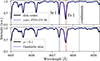 |
Fig. 1. Intensity spectra at disk center and close to the limb compared to the FTS atlas (Neckel 1999, convolved with a 10 mÅ Gaussian and adding 5% stray light) and the Second Solar Spectrum atlas (Gandorfer 2002), respectively. Vertical dashed black lines indicate the spectral positions of the line cores (Sr I and Fe I) and the selected continuum position. Vertical red lines indicate the wavelength positions of the red wing where Stokes V/I is plotted later in the paper. We normalized each spectrum to the continuum. |
The observed spectral window lacks intrinsically unpolarized telluric lines, which limits direct validation of this correction. Additionally, some of the observed solar regions were far from the disk center, weakening the assumption of an unpolarized continuum necessary for the ad-hoc method. Instead of direct validation, we convince ourselves a posteriori of the efficiency of our full data processing pipeline by comparing the fractional linear polarization in the spectral lines of our data with the Second Solar Spectrum atlas (Gandorfer 2002), as discussed later in the text.
The reference direction for the linear polarization was rotated to make +Q parallel to the nearest solar limb. To perform this rotation, we calculated the angle between the solar rotation axis and the line connecting each spatial pixel to the center of the solar disk. This angle was derived from the helioprojective-cartesian coordinates available in the data headers and using the small-angle approximation (Thompson 2006). It is noted in the data caveats that the accuracy of the reported coordinates is relatively low7. Because of the limited observed FoV, it could not be reliably correlated with context images (e.g., from the Visible Context Imager, VBI; Wöger et al. 2021) for improving the coordinate accuracy of the μ = 0.74 dataset. The estimated accuracy of these coordinates is about 7″, based on our own limb observations (see next section). However, this number is likely a lower limit and the true error may be closer to 10″. Limited coordinate accuracy can introduce residual rotation between Q and U. This rotation is negligible near the solar limb, where the relative error of the angle is low, but becomes increasingly relevant closer to disk center, where small angular errors have a larger impact.
For consistency with scattering polarization observations presented in the literature, the polarization profiles were normalized to the corresponding intensity profile at each pixel. Throughout this paper, we therefore present and discuss fractional polarization values, though for simplicity we refer to them simply as “polarization”.
The absolute polarization level measured with the current ViSP observations has not yet been fully validated, hindering the determination of the continuum polarization level (e.g., Fluri & Stenflo 1999; Trujillo Bueno & Shchukina 2009). To avoid potential misinterpretations, we forced the continuum in all polarization states to zero. This was achieved by subtracting the mean polarization value in a spectral window of about 150 mÅ around the identified continuum point (to reduce statistical noise) from all wavelength points, for each polarized Stokes parameter and each spatial pixel separately8. Despite these corrections, small residual artifacts remained in the spectral lines. These are mainly visible in regions where the scattering polarization signal is intrinsically weak, such as near disk center, where even relatively minor artifacts become noticeable. Based on their spectral shape, we attribute these artifacts to a combination of known instrumental errors. One contributing factor is the intensity imbalance between the two orthogonally polarized beams in the dual-beam set-up, which was about a factor of 1.7. This imbalance arises primarily from the grating polarization and, to a lesser extent, the imperfect contrast of the analyzing polarizer. Such imbalances amplify errors in one beam relative to the other in dual-beam data reduction, as previously noted by Casini et al. (2012) and de Wijn et al. (2022), and are known to reduce dual-beam polarimetric efficiency.
Although all calibration steps are incorporated in the data reduction pipeline and the measured polarimetric efficiencies fall within expected ranges, some level of uncertainty remains inherent to any polarimetric data processing. ViSP was known to exhibit internal ghosting9 from multiple reflections, which vary with arm and wavelength. In our analysis, we control for potential ghost-related artifacts by performing a comparative assessment using the Fe I line.
For the subsequent analysis of intensity and linear polarization Stokes maps, we focus on three fixed wavelength points: the core of Sr I, the core of Fe I10, and the continuum. These points, indicated with black dashed vertical lines in Fig. 1, are determined from the spatial mean intensity of each dataset, and are used consistently throughout our analysis rather than selecting, for example, the maximum polarization value. The latter is ill-defined in the presence of noise and can vary unpredictably across pixels.
An alternative approach is to track the Doppler-shifted spectral line core for each pixel. While this method did not alter our qualitative conclusions, we observed a slightly different noise distribution, shifted and broadened toward higher values. We attribute this to the fact that, in the Doppler-shifted approach, polarization values are sampled from various detector pixels on the ViSP sCMOS camera, each with its own noise characteristics. In contrast, the fixed-wavelength method uses a consistent pixel across the dataset, minimizing pixel-to-pixel noise variation and avoids assumptions on the yet unconstrained spectral shape of the Sr I line polarization at high spatial resolution. While this approach may not fully exploit the spectral coherence of the data, it provides a conservative and reproducible reference for comparing future observations and simulations. For simplicity, we refer to the specific wavelengths as Sr I, Fe I, and the continuum. To ensure the reliability of our findings in the following sections, all Sr I signals are consistently compared to reference signals in the neighboring Fe I line and continuum. If not stated otherwise, the intensity is normalized arbitrarily.
Since the Stokes V/I signals due to the longitudinal Zeeman effect in the absence of velocities are expected to be small in the line core, we decided to show the maps of V/I in the red wing of the spectral lines. The offset from the line cores is 45.5 mÅ, and the position is indicated by the vertical dashed red lines in Fig. 1.
While the line depths of the intensity spectra at disk center differ by approximately 20% from the Fourier Transform Spectrometer (FTS) atlas by Neckel (1999), the agreement improves substantially when the FTS profiles are convolved with a Gaussian of standard deviation 10 mÅ and supplemented with a 5% stray light contribution11. Near the limb, the ViSP spectra already show good agreement with the limb atlas by Gandorfer (2002), see Fig. 1. Since the FTS atlas is effectively free of spectral stray light, this moderately good agreement suggests that spectral stray light in ViSP is low but not negligible at this wavelength. Given that DKIST and ViSP were designed for high-sensitivity observations of faint coronal and prominence structures (de Wijn et al. 2022), the residual stray light may originate from known internal ghosting in this optical arm.
In contrast, the comparison with the limb atlas by Gandorfer (2002) is less straightforward. The line depths in the atlas are shaped by several factors, such as limb distance, spectral resolution, and stray light, which makes it difficult to determine the individual contribution of each. Consequently, the close agreement between the line depths of ViSP and the limb atlas may be coincidental.
3. Results
In this section, we present the observed and processed data as described in the previous section. We present full Stokes spectrograms at disk center in Section 3.1. From the limb dataset, we present full Stokes spatial maps and the center-to-limb variation (CLV) of the intensity and linear polarization in Section 3.2. Finally, we present full Stokes spatial maps at limb distance μ = 0.74 in Section 3.3. For the the maps at limb distance μ = 0.74, we analyze the spatial distribution of the total linear polarization with respect to the photospheric structures given by the continuum intensity and line-of-sight (LOS) velocity. Finally, we estimate the spatial signal-to-noise distribution.
3.1. Disk center
Figure 2 shows the spectrograms in Stokes I, Q/I, U/I, and V/I at disk center (μ = 0.998) including both the Sr I and the neighboring Fe I lines. As expected, the V/I spectra show the characteristic weak longitudinal Zeeman signals. In contrast, the linear polarization signals exhibit weak but systematic structures. In both Sr I and Fe I, the Q/I and U/I spectra display V-like signatures, with one positive and one negative lobe (i.e., antisymmetric features) across the line profiles. These cannot be attributed to cross-talk from V/I into Q/I or U/I, as there is no significant correlation between these patterns and the circular polarization signal. Given the magnetically relatively quiet conditions (as inferred from the low V/I amplitudes), we attribute these signatures to instrumental effects. They are not consistent with transverse Zeeman effect signatures or intensity cross-talk. As pointed out in Section 2.2, the likely origin are instrumental limitations, which may leave residual polarization artifacts in the data. Since these non-solar features dominate the linear polarization, we did not analyze this dataset further.
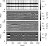 |
Fig. 2. Full Stokes spectrograms of the first scan and fifth slit position at disk center, clipped to the spectral region of Sr I (bottom spectral line) and Fe I (top spectral line). |
3.2. Limb
The dataset at the limb contains three scans with similar image quality. We investigate low spatial resolution spectra and the center-to-limb variation at high spatial resolution in Sections 3.2.1 and 3.2.2, respectively.
3.2.1. Limb spectra
To analyze the Q/I spectra, we average all three scans and scan positions, which results in a low spatio-temporal resolution in the direction perpendicular to the slit, specifically in the radial direction. We show the individual limb scans in Sr I in Appendix A. From the continuum intensity distribution along the slit, which includes the limb because the slit is perpendicular to it, we determine the limb distance for each pixel along the slit12. The linear polarization spectra at several limb distances are shown in Fig. 3.
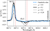 |
Fig. 3. Linearly polarized spectra (obtained as explained in the text) at different limb positions μ (see legend). For reference, the data from the Second Solar Spectrum atlas (Gandorfer 2002) are also shown. |
In terms of spectral shape, the linear polarization signal in Sr I exhibits the characteristic single-lobed profile expected from scattering polarization and according to theoretical calculations. For lines that present scattering polarization, including the Sr I line, the linear polarization signal is highly sensitive to the limb distance, with polarization amplitudes increasing towards the limb. The maximum linear polarization at the extreme limb (μ = 0.0) is 1.27%, which is significantly lower than what was reported by Stenflo et al. (1997, up to 2%). The figure also shows the linear polarization reported in the Second Solar Spectrum atlas by Gandorfer (2002), where we removed the continuum polarization for compatibility with our data. Their measured linear polarization parallel to the limb is slightly lower than what we find in our dataset. Their stated limb distance is μ = 0.1, but with limited accuracy, as the observations of Gandorfer (2002) were obtained before active limb tracking became available at IRSOL. Note that the spectral resolution of the atlas is 5 mÅ and therefore higher than in the ViSP data. Therefore, small discrepancies in the linear polarization amplitude are expected. Similar to the atlas, the neighboring Fe I line slightly depolarizes the continuum (Stenflo et al. 1997), although at the extreme limb the depolarization is more pronounced.
3.2.2. Spatial Stokes maps at the limb
Figure 4 presents spatial Stokes maps of Sr I, Fe I, and the continuum (top panels), along with the CLV of intensity and Q/I (bottom panels). The maps are averaged over all three available scans, which look similar in intensity and Q/I, representing a temporal integration of 30 minutes. This reduces statistical noise, and makes our results more easily comparable with previous studies. However, linear polarization fine structures that are clearly visible in the single scans of Sr I (see Appendix A) are lost when averaging. Due to the limited scan width relative to the slit length, the aspect ratio between the horizontal and vertical axes is strongly distorted, approximately 1:60. Iso-contours of μ are overplotted, where μ = 0 is given by the inflection point of the continuum intensity profile along the limb direction. The nominal solar limb position from ViSP’s coordinates given in the headers is also indicated in the continuum intensity panel, showing an offset of approximately 7″.
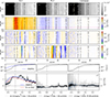 |
Fig. 4. Four upper rows: Full Stokes maps for Sr I (left column), Fe I (central column), and the continuum (right column), averaged over all three scans and spatially binned to 0 |


The on-disk Stokes maps in the continuum are free from any features, which gives us confidence that intensity cross-talk was sufficiently removed during the data reduction process. The bright point at μ = 0.18 induces noticeable transverse Zeeman signals in Q/I and longitudinal Zeeman signals in V/I for the spectral lines. The Q/I maps in Sr I and Fe I show the CLV behavior already discussed in the previous section. Interestingly, some linear polarization is visible beyond the limb position. We discuss this aspect further below.
The U/I maps in Sr I and Fe I show both positive and negative signals. However, they are only slightly larger in Sr I than in Fe I. This could be due to temporal cancellation, because the single scans exhibit significantly stronger signals in Sr I. However, it is difficult to determine the extent to which the Sr IU/I signal arises from radiative transfer-induced polarization – produced by scattering of anisotropic radiation and by velocity gradients even in the absence of magnetic fields (see del Pino Alemán et al. 2018) – or from Hanle rotation (Zeuner et al. 2022), noting that a contribution from the transverse Zeeman effect cannot be excluded. The only way to distinguish between the Hanle and Zeeman effects would be to look at the spectra. However, only some spectra in the FoV have an unambiguous single-lobe profiles in Sr I. Although likely small, residual rotation between Q/I and U/I cannot be excluded completely, as discussed in Section 2.2. Given these challenges, we leave a further investigation and interpretation of the Q/I and U/I signals in terms of the Hanle effect for a future work.
Comparing the CLV of the Sr I intensity shown in the second-last row of Fig. 4 to the one shown in the ZIMPOL data taken at the Gregory-Coudé telescope of the IRSOL observatory (0.45 m aperture; Zeuner et al. 2022)13, one can notice that the limb in DKIST is significantly sharper. This likely results from DKIST’s very low stray light levels (it was designed as a coronograph) and its adaptive optics system, which stabilizes the limb position far more effectively than is possible at IRSOL. In the bottom row of Fig. 4, we report the CLV of Q/I in the core of Sr I from our analyzed ViSP dataset, ZIMPOL, and a low spatial resolution observation taken at Pic du Midi (continuum polarization is subtracted; Malherbe 2025)14. For ViSP, we show the CLV at three levels of spatial averaging: a single scan at a single slit position (no averaging), all scans averaged at that slit position, and an average over all scans and slit positions. The selected slit position is marked by the horizontal dashed pink line in the Q/I image panels. All three ViSP observations show similar CLV trends. Compared to ViSP and ZIMPOL, the Pic du Midi amplitudes are slightly lower. A notable feature in all datasets is a local minimum in linear polarization very close to the limb in Sr I. The Q/I signal drops sharply just outside the limb, a behavior also observed in molecular lines presented by Milić & Faurobert (2012). As shown by the authors, this steep decline can be attributed to the sphericity of the solar atmosphere. Remarkably, the general trend of the spatially averaged Q/I CLV (black curve) is highly compatible with ZIMPOL data (Zeuner et al. 2022), especially at the extreme limb (μ = 0). However, the small-scale fluctuations are much more pronounced for ViSP, which is probably a result of the low spatio-temporal resolution of the ZIMPOL measurement. Also, the ZIMPOL Q/I CLV shows scattering polarization signals further beyond of the limb, probably due to the point-spread function already affecting the intensity.
3.3. Spatial Stokes maps at μ = 0.74
From the intensity image of this observation, a spatial resolution of 0 2 was determined by Zeuner et al. (2025). To improve the signal-to-noise (S/N) while preserving spatial information, we thus applied a spatial binning of 0
 1. This results in a final spatial sampling of 0
 1 × 0
1 × 0 1. In Appendix B, a VBI context image in the 4500 Å continuum15 is provided for illustrative purposes, noting that the limited FoV of ViSP does not allow accurate co-alignment.
3.3.1. Noise estimation
Before the binning, the spatial standard deviation (which we call noise) in the continuum linear polarization is σ = 0.032% at a single spectral point. After binning, the noise level in the continuum for the linear polarization is approximately σb≈ 0.014%. This value is slightly higher than the expected 0.011% derived from the unbinned data, assuming only statistical photon noise is present. The discrepancy suggests additional systematic errors may be present in the spatial dimension of the camera. To account for these systematic effects when estimating the line-core noise from the continuum’s noise, we apply a correction factor larger than one, ensuring that the true noise level is not underestimated. This factor reflects the observed discrepancy, which can reach up to nearly a factor of two for large binning values (used only to test the noise-scaling behavior), between the measured continuum noise and the photon-noise expectation. Its empirical justification is discussed in Sect. 3.3.2.
For pure photon noise, the standard deviation in Sr I should scale with  , where l is the continuum-to-line-depth-ratio. Averaged over the full field of view, we find
  for Sr I. Including a worst-case correction factor of two, we obtain for the binned linear polarization an expected noise level of
  .
.
To estimate the noise in the total linear polarization defined as ![Mathematical equation: $ P_\mathrm{L} = \left[\left(Q/I\right)^2 + \left(U/I\right)^2\right]^{1/2} $](/articles/aa/full_html/2026/04/aa56974-25/aa56974-25-eq15.gif) in Sr I and Fe I from the continuum, we note that if the underlying distribution is normal, PL follows a half-normal distribution. However, we find that the observed distribution PL, cont in the continuum already deviates from this form: the ratio of the standard deviation σP to the mean ⟨PL, cont⟩ is 0.5 instead of the theoretical approximately 0.8. This again points to the presence of systematic errors, implying that σP is underestimated relative to the mean of the distribution.
in Sr I and Fe I from the continuum, we note that if the underlying distribution is normal, PL follows a half-normal distribution. However, we find that the observed distribution PL, cont in the continuum already deviates from this form: the ratio of the standard deviation σP to the mean ⟨PL, cont⟩ is 0.5 instead of the theoretical approximately 0.8. This again points to the presence of systematic errors, implying that σP is underestimated relative to the mean of the distribution.
We therefore construct a zero-signal reference distribution, i.e., a synthetic distribution representing the noise-only case,  , and define the noise value as
  . By using the mean of this distribution rather than its standard deviation, we obtain a conservative upper limit for the noise in the line core, since systematic tails in the distribution make the standard deviation an unreliable estimator in our case. An analogous definition is applied to Fe I. For the binned case, we use the binned continuum distribution PL, cont, b as the starting point for constructing the zero-signal reference. For the binned total linear polarization, this yields
  .
.
3.3.2. Spatial variation of polarization
Of the two scans conducted for the position at μ = 0.74, we focus our analysis of the spatial variation of the total linear polarization on the one scan with the best image quality. Figure 5 presents the spatially binned Stokes maps of the quiet Sun region scanned by ViSP for Sr I, Fe I, and the continuum, respectively. Although the view is projected at μ = 0.74, solar granulation remains clearly visible in the intensity continuum image. A strong resemblance between Sr I and Fe I is noticeable in the intensity images, indicating that both lines probe similar atmospheric depths. The Stokes V/I maps also appear similar in shape. Differences in the amplitude can be attributed to different Landé factors. If the linear polarization signals in Sr I were solely due to the Zeeman effect or systematic errors, we would expect its linear polarization pattern to closely follow that of Fe I. However, both the signal amplitudes and structures differ significantly, indicating that the Sr I polarization is not merely a result of Zeeman signals or residual data processing artifacts.
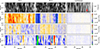 |
Fig. 5. Full Stokes maps in Sr I, Fe I, and continuum from ViSP scanning of a 61 |


Remarkable fine structure is visible below the spatial scales of one arcsec, in Q/I as well as in U/I. There appears to be a slight preference for positive U/I values on the left and negative values on the right side of the slit center. This pattern may indicate a residual from an imperfect rotation between Q/I and U/I, as discussed in Section 2.2. This effect is more apparent in the Sr I line, where the scattering polarization tends to produce a predominantly positive Q/I signal. An imperfect rotation would therefore leak some of this signal into U/I, creating an artificial asymmetry. In contrast, Fe I does not exhibit the same positive bias in Q/I, making such rotation residuals less pronounced. The presence of a similar trend in Fe IU/I nonetheless suggests that an additional physical contribution – such as transverse Zeeman signals superimposed on the scattering polarization – might also be at play. The spatial average ⟨Q/I⟩ is 0.12% in Sr I, whereas for ⟨U/I⟩ it is below the noise level of σSr, b. Both spatially averaged linear polarization values in Fe I are below the expected noise level. The continuum polarization is free from any small-scale structure (e.g., resembling structures found in the intensity image), indicating that seeing-induced cross-talk is below the noise level.
The observed region is magnetically very quiet, as indicated by the low V/I signal in Fe I. We remind the reader that this image is taken in the red wing and not in the core of the line (vertical dashed red lines in Figs. 1 and 3). V/I is sensitive to the LOS magnetic field via the longitudinal Zeeman effect and does not exceed 1.5% in absolute value anywhere in the spectrum for the entire FoV. Since both Fe I spectral lines have a larger effective Landé factor than Sr I16, they are more sensitive to magnetic fields. Thus, the low polarization amplitudes in Fe I provide a robust reference for confirming the absence of significant LOS magnetic fields in this region.
As residual rotation between Q/I and U/I cannot be entirely ruled out (see Section 2.2), hereafter we focus our analysis to the total linear polarization PL in Sr I and Fe I, to estimate which parts of the FoV exhibit more linear polarization than others. To explore how PL relates to granular structures in the photosphere, we examine its spatial distribution. Our scanned FoV is too small to apply standard granule segmentation techniques reliably (e.g., Liu et al. 2021; Díaz Castillo et al. 2022). Instead, we classify granules and intergranular lanes using a combination of continuum intensity and the LOS velocity vlos. The LOS velocity is calculated from the Doppler induced line shifts in Sr I, where the zero is the spatial mean line core position. Thereby we ignore Doppler shifts due to the solar rotation. We note that the inferred LOS velocities (also in the core of the Fe I line) appear lower than values commonly reported for high spatial resolution observations. This is expected given the achieved spatial resolution of  and minor stray light contributions. While these effects reduce the apparent amplitude of granular velocities, the exact velocity values are not critical for the classification used here. Unlike previous studies (e.g., Malherbe et al. 2007; Zeuner et al. 2018; Dhara et al. 2019), which relied solely on continuum intensity, by incorporating Doppler velocity information we thereby account for some projection effects and add more robustness to the classification into granules or intergranules. This is particularly relevant at our off-center viewing angle.
We emphasize that our classification does not imply that a granular (intergranular) pixel definitely belongs to a granule (intergranule). Instead, we use the terms granule and intergranule to describe pixels that exhibit characteristic properties: brightness in the continuum intensity and negative LOS velocities for granules, or darkness and positive LOS velocities for intergranules. Figure 6 shows a scatter plot of continuum intensity versus the LOS velocity for all pixels. We apply a threshold-based segmentation using two thresholds for each property; the four thresholds are indicated by dashed lines in the figure. The choice of the threshold values is discussed later. From this classification, we select three categories of pixels: granular (green), intergranular (black), and a boundary group (purple), which includes pixels that are neither particularly bright/dark nor exhibit significant Doppler shifts17. Using this classification, we compute normalized histograms (hereafter just histograms) of total linear polarization for each group, as shown in Fig. 7.
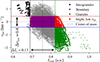 |
Fig. 6. Scatter plot of the continuum intensity and LOS velocity estimated from Sr I for μ = 0.74. Vertical dashed black and green lines indicate the positions of the intensity thresholds for the intergranules and granules, respectively. Horizontal dashed red and blue lines indicate the LOS velocity thresholds for intergranules and granules, respectively. The choice of the thresholds are given in the main text. |
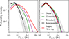 |
Fig. 7. Histograms of the total linear polarization of different pixel categories in the Sr I (left) and in the Fe I (right) line cores. The categories are given by thresholds in the continuum intensity and vlos (see text for details). The noise distributions (gray area) are the zero-signal reference distributions PL, zero (see text for details). |
The central dashed gray line marks the noise calculated with the spatially averaged line depths in the zero-signal distribution PL, zero explained in the previous section, while the upper and lower limits take into account the range of line depths throughout the FoV. This provides an estimate of the minimum and maximum polarization noise levels expected in our data, serving as a reference for interpreting signal significance. Because binning may distort the noise distribution (see previous section), the histograms are constructed from unbinned data to ensure accurate noise representation.
For Fe I, the total linear polarization in all categories closely follows the estimated noise distribution, indicating no significant polarization signal above noise. This agreement confirms that our noise estimation method is consistent with the observed data. In particular, it validates the correction factor of two introduced in the previous section, which compensates for the additional broadening of the noise distribution beyond that expected from pure photon statistics. In contrast, for Sr I, both boundary and granular categories exhibit significant total linear polarization, substantially exceeding the estimated noise, while only the intergranular category shows polarization levels consistent with the noise distribution. This reinforces that our estimated noise level is realistic and that the enhanced Sr I signals cannot be attributed to noise misestimation. We found that the continuum intensity threshold used to define intergranules notably affects the Sr I results.
We set the lower continuum threshold to include enough intergranular pixels for robust statistics, while avoiding the inclusion of pixels that would shift the polarization probability density of this category toward higher values, thereby keeping it consistent with noise. Even so, only about 350 pixels meet our intergranular criteria, and therefore, the corresponding histogram (black line) is truncated at the 10−2 level. In contrast, the polarization signals in the granule and boundary category are largely insensitive to variations in the upper continuum threshold, suggesting robustness of the total linear polarization above the noise in those categories. However, depending on the chosen continuum thresholds, the granule and boundary categories may yield nearly identical histograms. Sensitivity tests indicate that our findings are weakly dependent on the precise LOS velocity thresholds used.
Interestingly, the highest total linear polarization values are found in pixels that do not fall into any of the three main classifications (intergranule, boundary, or granule). Specifically, bright pixels with low LOS velocities – highlighted in red in Fig. 6 – exhibit significantly stronger total linear polarization than either granules or boundary categories (see red line in Fig. 7). This result is largely insensitive to the specific threshold values chosen. Nonetheless, we selected thresholds that maximize the total linear polarization signal within this category. We refer to this category as bright, low vlos pixels. Likely, they correspond to the overturning zone in simplified models of granulation. This aspect is discussed in Section 4. The spatial mean of the total linear polarization in the granular transition is 1.8 times stronger than in the intergranules. The remaining intermediate classes were also examined; their polarization distributions show no distinctive behavior, lying between those of interganular and bright, low vlos pixels.
3.3.3. S/N distribution
To assess the spatial scales of total linear polarization at different S/N thresholds, we analyze the total linear polarization in Sr I using S/N =  levels of 2, 3, and 4. A representative subregion of the full map is shown in Fig. 8, where contours corresponding to these S/N levels are overlaid on both the Sr I and Fe I total linear polarization maps. This zoomed-in view highlights the fine structure of the polarization signals, particularly in Sr I. We compute the spatial mean of the total linear polarization ⟨PL⟩ between successive S/N levels. To ensure the robustness of our results, we also calculate the spatial median, which closely matches the mean – indicating the distribution is not strongly skewed by outliers. The results are summarized in Table 1, which lists the mean total linear polarization amplitudes for both Sr I and Fe I.
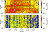 |
Fig. 8. Total linear polarization maps for Sr I (upper panel) and Fe I (lower panel) with contours at the S/N = PL, Sr, b/σSr, bP levels 2, 3, and 4, indicated by the line colors black, green, and cyan, respectively, for a detailed region of Fig. 5 at μ = 0.74. |
Spatially averaged total linear polarization and covered fractional area at different signal-to-noise levels given by Sr I.
Even at the highest S/N levels, the Fe I structures remain close to the noise level. This suggests the distinct physical origin of the scattering polarization in Sr I, in contrast to the magnetically sensitive Zeeman signals that dominate Fe I. In particular, polarization signals in Sr I cannot be attributed to transverse Zeeman signals (which might be present even in the very quiet Sun), systematic errors, or instrumental cross-talk alone.
Additionally, we assess the fractional area fa covered by total linear polarization signals in Sr I at each S/N level, which may serve as a proxy for the spatial filling factor of scattering polarization signals associated with small-scale structures. These coverage fractions are listed in Table 1. About 40% of the pixels on the FoV have a S/N of less than 2. Notably, only 0.25% of the FoV shows total linear polarization signals with a S/N greater than 4, highlighting the highly localized nature of strongly polarized features. In terms of spatial extent, these structures are smaller than 0 5 and reach polarization amplitudes of up to 0.42% (see cyan contours in Fig. 8). As expected, the typical size of polarized features decreases with increasing S/N, implying that the strongest signals are associated with the smallest structures. del Pino Alemán et al. (2018) also found that a reduction of spatial resolution results in lower polarization amplitudes. These findings emphasize the need for higher S/N across a larger portion of the FoV to enable detailed studies of the spatial distribution of scattering polarization. At the same time, preserving high spatial resolution is critical, because the most significant polarization signals are concentrated in relatively small areas.
4. Discussion and conclusions
Our observations of the Sr I 4607 Å line for μ = 0.74 show clear spatial structuring in the linear polarization, particularly in U/I, with alternating positive and negative values. The absence of similar spatial patterns in Fe I suggests that the observed polarization structure in Sr I arises mainly from scattering and possibly the Hanle effect rather than the Zeeman effect or instrumental artifacts. This spatial structure, consistent with earlier theoretical work (Trujillo Bueno & Shchukina 2007; del Pino Alemán et al. 2018), results in an average U/I signal close to zero. The agreement with these predictions reinforces the role of symmetry-breaking effects in shaping the scattering polarization.
The enhanced spatial resolution of our ViSP observations (down to ∼0 2, see Zeuner et al. 2025) reveals sub-arcsecond-scale polarization features that remained partially unresolved in earlier studies, such as Zeuner et al. (2020), where the spatial resolution was approximately twice as coarse. These findings provide a valuable observational benchmark for testing radiative transfer calculations in quiet Sun models resulting from three-dimensional magneto-convection simulations. A key result of this study is the detection of enhanced total linear polarization (PL, Sr) in granular and boundary categories compared to the intergranular category at μ = 0.74. In the most extreme intergranular cases (i.e., dark, strongly redshifted, pixels), polarization signals are compatible with the noise level as defined by our criteria. This observation supports theoretical predictions (Trujillo Bueno & Shchukina 2007; del Pino Alemán et al. 2018) that the quiet Sun scattering polarization is non-uniform and modulated by the granulation. Moreover, this result is compatible with previous spectrograph observations. These observations (Malherbe et al. 2007; Bianda et al. 2018; Dhara et al. 2019) similarly reported positive correlations between Q/I and continuum intensity, independent of the limb distance with μ > 0.2. They interpreted this result as enhanced scattering polarization in granules relative to intergranules, likely due to stronger magnetic depolarization in the latter regions via the Hanle effect. On the other hand, the opposite trend has been found in filtergraph observations at μ = 0.6 (Zeuner et al. 2018). They found an anticorrelation of Q/I with the continuum intensity. Rigorously comparing our results with such filtergraph observations would require taking into account a sufficient spatial and spectral degradation of the polarized spectra, which are currently limited by the systematic errors.
For our observation, the suppression of PL, Sr in the intergranular group may be interpreted in two ways: either intergranules are weakly polarized due to a higher degree of axial symmetry, or the signals are depolarized via the Hanle effect. The first explanation, that intergranules are more axially symmetric, is not straightforward. If the identified structures are indeed intergranular lanes, one would typically expect them to exhibit less axial symmetry than granules. This is because plasma conditions are expected to change more abruptly across the intergranule (i.e., toward the neighboring granule) than along it. Indeed, at disk center, intergranular lanes often show enhanced scattering polarization precisely due to this increased asymmetry (Trujillo Bueno & Shchukina 2007; del Pino Alemán et al. 2018). Therefore, attributing the lower polarization to a higher degree of axial symmetry would require a more detailed physical justification, which is currently lacking. In contrast, the Hanle depolarization hypothesis offers a more consistent explanation within our current understanding, especially given the known sensitivity of Sr I to weak, unresolved magnetic fields. However, we cannot rule out that both explanations are present simultaneously. Disentangling these possibilities with a definitive interpretation of which is the dominant physical process that causes this difference would require a careful comparison with simulations including full 3D polarized radiative transfer in a realistic magnetohydrodynamic model, such as those of del Pino Alemán et al. (2018). Such simulations can determine whether magnetic depolarization is expected in pixels matching our intergranular definition. However, such a study is beyond the scope of this work.
An additional complication for interpretation is that, away from disk center, the classification into granules and intergranules based on the continuum intensity alone can be compromised by projection effects. Here, to improve the classification, we combined continuum intensity and Doppler velocity criteria. This dual-criteria method better accounts for projection effects closer to the limb, although foreshortening still introduces uncertainties, because even granular centers may appear red-shifted due to the projection of vertical flows (Oba et al. 2020), complicating the interpretation. Ultimately, more reliable classifications will require disk-center observations.
Interestingly, we detect the largest PL, Sr in bright pixels with weak LOS velocities, likely part of the overturning zone of granules. This zone at the edge of granules exhibits, on average, 80% stronger total linear polarization signals than found in the intergranular category. We speculate that the observed scattering polarization in the photosphere may be most efficiently generated in overturning zones, where strong horizontal and vertical velocity gradients coexist. The symmetry breaking caused by such velocity structures provides a physical mechanism for enhancing the scattering polarization signals. The role of horizontal velocity shear in scattering polarization generation has been emphasized by del Pino Alemán et al. (2018), and the formation of these gradients has been linked to baroclinic vorticity generation in granular boundaries, as discussed by Nordlund et al. (2009).
Our noise analysis, based on constructing a zero-signal distribution, indicates that less than 1 % of the FoV contains PL, Sr, b signals with S/N > 4 in Sr I, while fewer than half of the pixels have S/N < 2. While this is sufficient to reveal fine structure, it also shows that a large portion of the data are still noise-dominated. The strongest PL, Sr, b signals are confined to sub-arcsecond structures (< 0 5) with amplitudes below 0.5%. These compact features occupy less than 0.2% of the FoV, underscoring the need for instruments that combine high polarimetric sensitivity with excellent spatial and spectral resolution. The quoted fractions depend on our choice to evaluate the polarization at a single wavelength point. Including multiple wavelength samples across the line profile could increase the effective sensitivity and thereby modify these statistics, potentially increasing the fraction of pixels exceeding a given S/N threshold. However, at high spatial resolution the detailed spectral shape of the scattering polarization signal is not yet well constrained, as it results from a complex interplay of magnetic fields, velocity gradients, anisotropic radiation, and collisions. Once physically motivated models and inversion techniques become available, combining information from multiple wavelength samples is expected to yield a significant improvement in effective S/N, as demonstrated by Díaz Baso et al. (2025).
Although doubling the integration time and ViSP’s camera duty cycle could improve the S/N by up to a factor of two, our analysis indicates that the current data may not be purely photon-noise limited. Residual instrumental effects, such as internal ghosts, likely contribute significantly and must be addressed in future observations to fully leverage ViSP’s polarimetric sensitivity. Recent optical improvements and testing with ViSP have shown improved stray light suppression and internal ghosting reduction from the initial commissioning datasets.
While some of the limiting factors that affect the current spatial resolution of ViSP can be mitigated, such as image jitter induced by vibrations due to laboratory instruments, others, including solar dynamics during exposure, pose fundamental limits. Nonetheless, the performance of ViSP demonstrates the feasibility of detecting weak scattering polarization signals in the quiet Sun and motivates further improvements. In particular, observations at disk center will help resolve ambiguities in the granule-intergranule classification, minimize foreshortening effects, and provide a more direct view of the vertical plasma dynamics. The combination of ViSP data with high-cadence context imaging and simulations promises to significantly advance our understanding of the coupling between plasma flows, tangled magnetic fields, and scattered radiation in the lower solar atmosphere.
Acknowledgments
We express our gratitude to the referee for providing valuable suggestions that have enhanced the clarity of the paper. We thank Thomas Schad for helpful discussions. F.Z. and L.B. acknowledge funding from the Swiss National Science Foundation under grant numbers PZ00P2_215963 and 200021_231308, respectively. T.P.A.’s participation in the publication is part of the Project RYC2021-034006-I, funded by MICIN/AEI/10.13039/501100011033, and the European Union “NextGenerationEU”/RTRP. T.P.A. and J.T.B. acknowledge support from the Agencia Estatal de Investigación del Ministerio de Ciencia, Innovación y Universidades (MCIU/AEI) under grant “Polarimetric Inference of Magnetic Fields” and the European Regional Development Fund (ERDF) with reference PID2022-136563NB-I00/10.13039/501100011033. E.A.B. acknowledges financial support from the European Research Council (ERC) through the Synergy grant No. 810218 (“The Whole Sun” ERC-2018-SyG). Work by R.C. was supported by the National Center for Atmospheric Research, which is a major facility sponsored by the National Science Foundation (NSF) under Cooperative Agreement No. 1852977. This research has made use of NASA’s Astrophysics Data System Bibliographic Services. The research reported herein is based in part on data collected with the Daniel K. Inouye Solar Telescope (DKIST), a facility of the National Solar Observatory (NSO). The NSO is managed by the Association of Universities for Research in Astronomy, Inc., and funded by the National Science Foundation. Any opinions, findings, and conclusions or recommendations expressed in this publication are those of the authors and do not necessarily reflect the views of the National Science Foundation or the Association of Universities for Research in Astronomy, Inc. DKIST is located on land of spiritual and cultural significance to Native Hawaiian people. The use of this important site to further scientific knowledge is done with appreciation and respect. The observational DKIST data used during this research is openly available from the DKIST Data Center Archive under the proposal identifier pid_2_70. Facilities: DKIST (Rimmele et al. 2022). Software: Astropy (The Astropy Collaboration 2022), Matplotlib (Hunter 2007), Numpy (Harris et al. 2020), SciPy (Virtanen et al. 2020), SunPy (Barnes et al. 2020).
References
- Barnes, W. T., Bobra, M. G., Christe, S. D., et al. 2020, ApJ, 890, 68 [Google Scholar]
- Bellot Rubio, L., & Orozco Suárez, D. 2019, Liv. Rev. Sol. Phys., 123 [Google Scholar]
- Bianda, M., Berdyugina, S., Gisler, D., et al. 2018, A&A, 614, A89 [NASA ADS] [CrossRef] [EDP Sciences] [Google Scholar]
- Casini, R., de Wijn, A. G., & Judge, P. G. 2012, ApJ, 757, 45 [Google Scholar]
- de Wijn, A. G., Casini, R., Carlile, A., et al. 2022, Sol. Phys., 297, 22 [NASA ADS] [CrossRef] [Google Scholar]
- del Pino Alemán, T., & Trujillo Bueno, J. 2021, ApJ, 909, 180 [CrossRef] [Google Scholar]
- del Pino Alemán, T., Trujillo Bueno, J., Štěpán, J., & Shchukina, N. 2018, ApJ, 863, 20 [CrossRef] [Google Scholar]
- Dhara, S. K., Capozzi, E., Gisler, D., et al. 2019, A&A, 630, A67 [NASA ADS] [CrossRef] [EDP Sciences] [Google Scholar]
- Díaz Baso, C. J., Milić, I., Rouppe van der Voort, L., & Schlichenmaier, R. 2025, A&A, 693, A272 [NASA ADS] [CrossRef] [EDP Sciences] [Google Scholar]
- Díaz Castillo, S. M., Asensio Ramos, A., Fischer, C. E., & Berdyugina, S. V. 2022, Front. Astron. Space Sci., 9, 1 [Google Scholar]
- Faurobert-Scholl, M. 1993, A&A, 268, 765 [NASA ADS] [Google Scholar]
- Faurobert-Scholl, M., Feautrier, N., Machefert, F., Petrovay, K., & Spielfiedel, A. 1995, A&A, 298, 289 [NASA ADS] [Google Scholar]
- Fluri, D. M., & Stenflo, J. O. 1999, A&A, 341, 902 [NASA ADS] [Google Scholar]
- Gandorfer, A. 2002, The Second Solar Spectrum: A high Spectral Resolution Polarimetric Survey of Scattering Polarization at the Solar Limb in Graphical Representation. Volume II: 3910 Å to 4630 Å (Zurich: VdF) [Google Scholar]
- Harrington, D. M., Sueoka, S. R., Schad, T. A., et al. 2023, Sol. Phys., 298, 10 [Google Scholar]
- Harris, C. R., Millman, K. J., van der Walt, S. J., et al. 2020, Nature, 585, 357 [NASA ADS] [CrossRef] [Google Scholar]
- Hunter, J. D. 2007, Comput. Sci. Eng., 9, 90 [NASA ADS] [CrossRef] [Google Scholar]
- Jaeggli, S. A., Schad, T. A., Tarr, L. A., & Harrington, D. M. 2022, ApJ, 930, 132 [Google Scholar]
- Kleint, L., Berdyugina, S. V., Shapiro, A. I., & Bianda, M. 2010, A&A, 524, A37 [NASA ADS] [CrossRef] [EDP Sciences] [Google Scholar]
- Landi Degl’Innocenti, E. 1982, Sol. Phys., 77, 285 [Google Scholar]
- Liu, Y., Jiang, C., Yuan, D., et al. 2021, ApJ, 923, 133 [Google Scholar]
- Malherbe, J. M. 2025, arXiv e-prints [arXiv:2505.17545] [Google Scholar]
- Malherbe, J.-M., Moity, J., Arnaud, J., & Roudier, T. 2007, A&A, 462, 753 [NASA ADS] [CrossRef] [EDP Sciences] [Google Scholar]
- Milić, I., & Faurobert, M. 2012, A&A, 539, A10 [NASA ADS] [CrossRef] [EDP Sciences] [Google Scholar]
- Neckel, H. 1999, Sol. Phys., 184, 421 [Google Scholar]
- Nordlund, Å., Stein, R. F., & Asplund, M. 2009, Liv. Rev. Sol. Phys., 6, 2 [Google Scholar]
- Oba, T., Iida, Y., & Shimizu, T. 2020, ApJ, 890, 141 [NASA ADS] [CrossRef] [Google Scholar]
- Rempel, M. 2014, ApJ, 789, 132 [Google Scholar]
- Rempel, M., Bhatia, T., Rubio, L. B., & Korpi-Lagg, M. J. 2023, Space Sci. Rev., 219, 36 [NASA ADS] [CrossRef] [Google Scholar]
- Rimmele, T. R., Warner, M., Keil, S. L., et al. 2020, Sol. Phys., 295, 172 [Google Scholar]
- Rimmele, T. R., Warner, M., Casini, R., et al. 2022, in Ground-based and Airborne Instrumentation for Astronomy IX, eds. H. K. Marshall, J. Spyromilio, & T. Usuda, (Montréal: SPIE), SPIE Conf. Ser., 12182, 121820Z [Google Scholar]
- Sanchez Almeida, J., & Lites, B. W. 1992, ApJ, 398, 359 [Google Scholar]
- Snik, F., de Wijn, A. G., Ichimoto, K., et al. 2010, A&A, 519, A18 [NASA ADS] [CrossRef] [EDP Sciences] [Google Scholar]
- Stenflo, J. O. 1982, Sol. Phys., 80, 209 [Google Scholar]
- Stenflo, J. O., Bianda, M., Keller, C. U., & Solanki, S. K. 1997, A&A, 322, 985 [NASA ADS] [Google Scholar]
- The Astropy Collaboration (Price-Whelan, A. M., et al.) 2022, ApJ, 935, 167 [NASA ADS] [CrossRef] [Google Scholar]
- Thompson, W. T. 2006, A&A, 449, 791 [NASA ADS] [CrossRef] [EDP Sciences] [Google Scholar]
- Trelles Arjona, J. C., Martínez González, M. J., & Ruiz Cobo, B. 2021, ApJ, 915, L20 [NASA ADS] [CrossRef] [Google Scholar]
- Trujillo Bueno, J., & Shchukina, N. 2007, ApJ, 664, L135 [Google Scholar]
- Trujillo Bueno, J., & Shchukina, N. 2009, ApJ, 694, 1364 [NASA ADS] [CrossRef] [Google Scholar]
- Trujillo Bueno, J., Shchukina, N., & Asensio Ramos, A. 2004, Nature, 430, 326 [Google Scholar]
- Trujillo Bueno, J., Asensio Ramos, A., & Shchukina, N. 2006, in Solar Polarization 4 ASP Conference Series, eds. B. W. Casini, & R. Lites, Astron. Soc. Pacific Conf. Ser., 358, 269 [Google Scholar]
- Virtanen, P., Gommers, R., Oliphant, T. E., et al. 2020, Nat. Methods, 17, 261 [Google Scholar]
- Vögler, A., & Schüssler, M. 2007, A&A, 465, L43 [Google Scholar]
- Wöger, F., Rimmele, T. R., Ferayorni, A., et al. 2021, Sol. Phys., 296, 145 [CrossRef] [Google Scholar]
- Zeuner, F., Feller, A., Iglesias, F. A., & Solanki, S. K. 2018, A&A, 619, A179 [NASA ADS] [CrossRef] [EDP Sciences] [Google Scholar]
- Zeuner, F., Manso Sainz, R., Feller, A., et al. 2020, ApJ, 893, L44 [NASA ADS] [CrossRef] [Google Scholar]
- Zeuner, F., Belluzzi, L., Guerreiro, N., Ramelli, R., & Bianda, M. 2022, A&A, 662, A46 [NASA ADS] [CrossRef] [EDP Sciences] [Google Scholar]
- Zeuner, F., del Pino Alemán, T., Trujillo Bueno, J., & Solanki, S. K. 2024, ApJ, 964, 10 [Google Scholar]
- Zeuner, F., Belluzzi, L., Alsina Ballester, E., et al. 2025, A&A, 703, L10 [NASA ADS] [CrossRef] [EDP Sciences] [Google Scholar]
Even with a five-minute integration, the polarization contrast remains considerable.
Ten modulation states accumulated 115 times with 12 ms exposure per state.
Product ID/Dataset ID: L1-LWINP/AJZRR
Product ID/Dataset ID: L1-WTXPV/BMNRV
Product ID/Dataset ID: L1-MIYID/AVXNW
Note that this step might introduce minor cross-talk from Stokes I near the limb, where some continuum polarization is expected; however, we find no evidence of this in our data.
See dataset caveats: https://nso.atlassian.net/wiki/spaces/DDCHD/pages/3481272321/ViSP+Data+Set+Caveats
In reality, this line is a blend of two Fe I transitions.
Based on the intensity profile, we estimate less than 1.5% scattered light at 15″ outside the limb as one contribution to the stray light.
We define the limb as the pixel with the largest continuum intensity gradient along the slit, that is, in radial direction.
The data are publicly available on ZENODO: https://zenodo.org/records/8087406.
The refractor was designed to be polarization free. The data are publicly available on HAL: https://cnrs.hal.science/hal-05076008.
Product ID/Dataset ID: L1-EBYNQ/BUQAXN
LS coupling assumed,  given by Landi Degl’Innocenti (1982):
  ,
,  and
and  .
.
Appendix A: Individual limb scans in Sr I
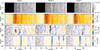 |
Fig. A.1. Full Stokes maps in Sr I for all three individual scans (from left to right, chronologically) spatially binned to 0 |


Appendix B: VBI context image at μ = 0.74
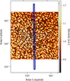 |
Fig. B.1. Co-temporal VBI context image at 4500 Å corresponding to the dataset at μ = 0.74, averaged over all frames belonging to the analyzed scan (10 min). The region scanned by ViSP is indicated in blue. Due to uncertainties in both the VBI coordinate accuracy and the co-alignment between VBI and ViSP, the indicated region is only approximate and intended for illustrative purposes. |
Appendix C: LoS velocity map at μ = 0.74
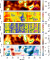 |
Fig. C.1. Intensity in Sr I (top) and total linear polarization maps (as explained in the main text) in Sr I, in Fe I (second and third panel, respectively), continuum intensity (second last panel) and LOS velocity (bottom panel) at μ = 0.74. Note the displayed region is a cutout from the full scan presented in Fig. 5, covering 13″. Contour colors are corresponding to the continuum intensity thresholds given in Fig. 6, separating dark (magenta lines) and bright (green lines) pixels. |
All Tables
Spatially averaged total linear polarization and covered fractional area at different signal-to-noise levels given by Sr I.
All Figures
|
Fig. 1. Intensity spectra at disk center and close to the limb compared to the FTS atlas (Neckel 1999, convolved with a 10 mÅ Gaussian and adding 5% stray light) and the Second Solar Spectrum atlas (Gandorfer 2002), respectively. Vertical dashed black lines indicate the spectral positions of the line cores (Sr I and Fe I) and the selected continuum position. Vertical red lines indicate the wavelength positions of the red wing where Stokes V/I is plotted later in the paper. We normalized each spectrum to the continuum. |
| In the text | |
|
Fig. 2. Full Stokes spectrograms of the first scan and fifth slit position at disk center, clipped to the spectral region of Sr I (bottom spectral line) and Fe I (top spectral line). |
| In the text | |
|
Fig. 3. Linearly polarized spectra (obtained as explained in the text) at different limb positions μ (see legend). For reference, the data from the Second Solar Spectrum atlas (Gandorfer 2002) are also shown. |
| In the text | |
|
Fig. 4. Four upper rows: Full Stokes maps for Sr I (left column), Fe I (central column), and the continuum (right column), averaged over all three scans and spatially binned to 0 |
| In the text | |
|
Fig. 5. Full Stokes maps in Sr I, Fe I, and continuum from ViSP scanning of a 61 |
| In the text | |
|
Fig. 6. Scatter plot of the continuum intensity and LOS velocity estimated from Sr I for μ = 0.74. Vertical dashed black and green lines indicate the positions of the intensity thresholds for the intergranules and granules, respectively. Horizontal dashed red and blue lines indicate the LOS velocity thresholds for intergranules and granules, respectively. The choice of the thresholds are given in the main text. |
| In the text | |
|
Fig. 7. Histograms of the total linear polarization of different pixel categories in the Sr I (left) and in the Fe I (right) line cores. The categories are given by thresholds in the continuum intensity and vlos (see text for details). The noise distributions (gray area) are the zero-signal reference distributions PL, zero (see text for details). |
| In the text | |
|
Fig. 8. Total linear polarization maps for Sr I (upper panel) and Fe I (lower panel) with contours at the S/N = PL, Sr, b/σSr, bP levels 2, 3, and 4, indicated by the line colors black, green, and cyan, respectively, for a detailed region of Fig. 5 at μ = 0.74. |
| In the text | |
|
Fig. A.1. Full Stokes maps in Sr I for all three individual scans (from left to right, chronologically) spatially binned to 0 |
| In the text | |
|
Fig. B.1. Co-temporal VBI context image at 4500 Å corresponding to the dataset at μ = 0.74, averaged over all frames belonging to the analyzed scan (10 min). The region scanned by ViSP is indicated in blue. Due to uncertainties in both the VBI coordinate accuracy and the co-alignment between VBI and ViSP, the indicated region is only approximate and intended for illustrative purposes. |
| In the text | |
|
Fig. C.1. Intensity in Sr I (top) and total linear polarization maps (as explained in the main text) in Sr I, in Fe I (second and third panel, respectively), continuum intensity (second last panel) and LOS velocity (bottom panel) at μ = 0.74. Note the displayed region is a cutout from the full scan presented in Fig. 5, covering 13″. Contour colors are corresponding to the continuum intensity thresholds given in Fig. 6, separating dark (magenta lines) and bright (green lines) pixels. |
| In the text | |
Current usage metrics show cumulative count of Article Views (full-text article views including HTML views, PDF and ePub downloads, according to the available data) and Abstracts Views on Vision4Press platform.
Data correspond to usage on the plateform after 2015. The current usage metrics is available 48-96 hours after online publication and is updated daily on week days.
Initial download of the metrics may take a while.