| Issue |
A&A
Volume 708, April 2026
|
|
|---|---|---|
| Article Number | A14 | |
| Number of page(s) | 24 | |
| Section | Cosmology (including clusters of galaxies) | |
| DOI | https://doi.org/10.1051/0004-6361/202557578 | |
| Published online | 25 March 2026 | |
Spectral properties of Anomalous Microwave Emission in 144 Galactic clouds
1
Instituto de Astrofísica de Canarias, 38200 La Laguna, Tenerife, Canary Islands, Spain
2
Departamento de Astrofísica, Universidad de La Laguna (ULL), 38206 La Laguna, Tenerife, Spain
3
Jodrell Bank Centre for Astrophysics, Alan Turing Building, Department of Physics and Astronomy, The University of Manchester, Oxford Road, Manchester M13 9PL, UK
4
Imperial College London, Blackett Lab, Prince Consort Road, London SW7 2AZ, UK
5
Consejo Superior de Investigaciones Científicas, Madrid, Spain
6
Instituto de Física de Cantabria (IFCA), CSIC-Univ. de Cantabria, Avenida de los Castros s/n, 39005 Santander, Spain
7
Laboratoire de Physique Subatomique et de Cosmologie, Université Grenoble Alpes, 53 Avenue des Martyrs Grenoble, France
8
Department of Physics, University of Oxford, Denys Wilkinson Building, Keble Road, Oxford OX1 3RH, UK
9
Cahill Centre for Astronomy and Astrophysics, California Institute of Technology, Pasadena, CA 91125, USA
★ Corresponding author: This email address is being protected from spambots. You need JavaScript enabled to view it.
Received:
7
October
2025
Accepted:
1
February
2026
Abstract
Anomalous Microwave Emission (AME) is a diffuse microwave component thought to arise from spinning dust grains, though it remains poorly understood. We analyzed AME in 144 Galactic clouds by combining low-frequency maps from S-PASS (2.3 GHz), C-BASS (4.76 GHz), and QUIJOTE (10–20 GHz) with 21 ancillary maps. Using aperture photometry and parametric spectral energy distribution (SED) fitting via Markov chain Monte Carlo methods without informative priors, we measured AME emissivity, peak frequency, and spectral width. We achieved peak frequency constraints nearly three times tighter than previous work and identify 83 new AME sources. The AME spectra are generally broader than predicted by spinning dust models for a single phase of the interstellar medium, suggesting either multiple spinning dust components along the line of sight or incomplete representation of the grain size distribution in current models. However, the narrowest observed widths match theoretical predictions, supporting the spinning dust hypothesis. The AME amplitude correlates most strongly with the thermal dust peak flux and radiance, showing ∼30% scatter and sublinear scaling, which suggests reduced AME efficiency in regions with brighter thermal dust emission. The AME peak frequency increases with thermal dust temperature in a trend current theoretical models do not reproduce, indicating that spinning dust models must incorporate dust evolution and radiative transfer in a self-consistent framework where environmental parameters and grain properties are interdependent. Polycyclic aromatic hydrocarbon tracers correlate with AME emissivity, supporting a physical link to small dust grains. Finally, a log-Gaussian function provides a good empirical description of the AME spectrum across the sample, given current data quality and frequency coverage.
Key words: radiation mechanisms: thermal / (ISM:) dust / extinction / cosmic background radiation / diffuse radiation / radio continuum: ISM
© The Authors 2026
 Open Access article, published by EDP Sciences, under the terms of the Creative Commons Attribution License (https://creativecommons.org/licenses/by/4.0), which permits unrestricted use, distribution, and reproduction in any medium, provided the original work is properly cited.
This article is published in open access under the Subscribe to Open model. This email address is being protected from spambots. You need JavaScript enabled to view it. to support open access publication.
1. Introduction
Anomalous Microwave Emission (AME) is a significant component of Galactic diffuse emission in intensity in the 10 < ν < 60 GHz range. It was discovered in CMB observations as excess emission strongly correlated with far-infrared radiation that could not be attributed to either synchrotron or free–free mechanisms (Kogut et al. 1996; Leitch et al. 1997; de Oliveira-Costa 1998). This correlation extends to scales as small as 2 arcmin, though most emission remains diffuse at larger angular scales (Watson et al. 2005; Casassus et al. 2008; Scaife et al. 2009; Dickinson et al. 2010; Tibbs et al. 2013; Battistelli et al. 2019; Arce-Tord et al. 2020; Harper et al. 2025). AME is widespread in our galaxy, accounting for up to half of the emission at 30 GHz (Planck Collaboration XXV 2016), and it is now recognized as a major CMB foreground in intensity, with even low levels of polarization potentially biasing cosmological constraints and challenging B-mode experiments (Remazeilles et al. 2016; Armitage-Caplan et al. 2012; Dunkley et al. 2009).
Observations of extragalactic sources have shown that AME is more concentrated in localized bubbles (Scaife et al. 2010; Murphy et al. 2010), where it can account for up to two thirds of the total emission (Hensley et al. 2015; Murphy et al. 2018). In the Andromeda galaxy, the overall contribution of AME remains an area of active research, and it is not yet clear whether its integrated emission is less dominant than that observed locally in the Milky Way (Fernández-Torreiro et al. 2024; Harper et al. 2023; Battistelli et al. 2019; Planck Collaboration XIII 2015).
The electric dipole spinning dust mechanism, first proposed by Erickson (1957) and developed by Draine & Lazarian (1998b), is the leading explanation for AME. In this model, dust grains with a component of an electric dipole moment in their spinning plane emit radiation at their rotational frequency. The emission is dominated by the smallest, fastest-spinning grains, which is why sub-nanometer-sized grains such as polycyclic aromatic hydrocarbons (PAHs; Draine & Lazarian 1998a), nanosilicates (Hensley et al. 2016; Hensley & Draine 2017), hydrogenated fullerenes (Iglesias-Groth 2005), and nanodiamonds (Greaves et al. 2018) have been proposed as primary carriers, with no conclusive evidence regarding the preference of a single carrier to date. Several refinements to the original Draine & Lazarian (1998a) model have been implemented in the IDL-based code SPDUST21 (Ali-Haïmoud et al. 2009; Ysard & Verstraete 2010; Hoang et al. 2010, 2011; Silsbee et al. 2011; Ali-Haïmoud 2010). The most recent development is the Python-based modelSPYDUST2 (Zhang & Chluba 2025), which generalizes the treatment of grain shapes.
A compelling argument for the spinning dust hypothesis is the lack of observed polarization. Many alternative mechanisms would produce measurable polarization, particularly at CMB frequencies (∼30–200 GHz), yet current upper limits on the polarization fraction are already ≈1% at 1° scales (Dickinson et al. 2011; López-Caraballo et al. 2011; Rubiño-Martín et al. 2012a; Génova-Santos et al. 2017; González-González et al. 2025) and a few percent at arcminute scales (Mason et al. 2009; Battistelli et al. 2015), with measurements primarily limited by instrumental systematics such as polarization leakage and residual background polarized synchrotron. Other potentially highly polarized mechanisms, such as magnetic dust emission (Draine & Hensley 2013; Hoang & Lazarian 2016), are thought to be present at higher frequencies and may be embedded in the low-frequency end of thermal dust emission, making them difficult to detect with current experiments. However, they could still pose a significant challenge in future B-mode experiments at the current limits (Dunkley et al. 2009; Remazeilles et al. 2016).
The characteristic bump of the spinning dust spectrum results from competing factors. While emitted power increases with the fourth power of rotational speed, the distribution of random excitations combined with damping establish a distribution of angular momenta that makes very high rotation rates rare, and the rapid growth of damping processes, especially electric dipole radiation, prevents grains from sustaining very high-frequency rotation. For a single grain, the spectral shape is well understood. However, for an astrophysical source, the observed spectrum is the sum of all individual grain spectra and therefore depends directly on the distributions of rotation rates, dipole moments, and the alignment between dipoles and rotation axes. These distributions are, in turn, influenced by grain sizes, shapes, compositions, and environmental conditions–specifically the intensity of the radiation field, gas temperature, and the abundances as well as ionization states of hydrogen and carbon, all of which are poorly known in practice.
Despite the success of spinning dust models in reproducing observed AME spectra, extracting grain parameters from observed spectral energy distributions (SEDs) remains a major challenge. This difficulty stems primarily from parameter degeneracy–many combinations of the eight required input parameters produce nearly identical spectral shapes. The problem is exacerbated by limited observational data, as current measurements have limited spectral coverage and are typically only sensitive to the upper part of spinning dust emission due to calibration systematics and limited sensitivity. Current theoretical models compound this problem by not accounting for the dynamical interplay between environmental parameters and grain characteristics. This limitation potentially allows for physically incompatible parameter combinations (e.g., a low gas temperature alongside a strong radiation field), and it ignores processes such as grain growth or fragmentation. Addressing these challenges would require a full radiative transfer model coupled with a dust evolution code such as DUSTEM (Compiègne et al. 2011), as demonstrated in Ysard et al. (2011). Additionally, the dimensionality of theoretical models would need to be reduced to directly fit SEDs, for example by using moment expansion methods as explored in recent work (Zhang & Chluba 2025) and originally introduced in Chluba et al. (2017).
Given these challenges, this paper adopts a simplified, phenomenological approach to modeling AME (outlined in Sect. 3.2.3). Our primary goal is to assess how changes in the AME spectrum correlate with changes in the physical environment. To this end, we measured SEDs for compact Galactic sources at 1° scales using aperture photometry, building on two previous studies. Planck Collaboration XV (2014) detected 42 significant AME sources out of 98, but the analysis was limited by sparse low-frequency data: In the southern sky there were no measurements between 2.3 and 22.8 GHz, and in the northern sky there were none between 1.42 and 22.8 GHz. More recently, Poidevin et al. (2023) identified 44 significant sources out of 52 and incorporated QUIJOTE data in the 10–20 GHz range, which greatly reduced biases in peak frequency and width. However, a substantial gap between 1.42 GHz and 11.1 GHz remained.
This paper presents a major improvement in low-frequency coverage by combining multiple datasets from QUIJOTE (Rubiño-Martín et al. 2023), C-BASS (Taylor et al., in prep.), and S-PASS (Carretti et al. 2019) in the context of the RadioForegrounds+ project3, We incorporate C-BASS data at 4.76 GHz in the northern hemisphere and S-PASS data at 2.3 GHz in the southern hemisphere, which enables accurate characterization of low-frequency foregrounds. This eliminates the need to fully rely on older large single-dish surveys with poorly understood beam characteristics and calibration. Additionally, the QUIJOTE data covering 11–19 GHz uniquely captures the low-frequency slope of the AME bump, allowing for more precise constraints on the peak frequency and width.
Together, these datasets allow us to fully constrain the AME amplitude, peak frequency, and width without applying informative priors, as shown in Cepeda-Arroita et al. (2021). By explicitly fitting for the width, we also reduce biases in peak frequency determination. The improved calibration of the new data allowed us to measure much fainter AME sources, expanding our analysis to 144 sources–significantly more than previous studies–including many at mid and high Galactic latitudes. In contrast, the two earlier studies primarily focused on sources near the Galactic plane.
This paper is organized as follows. Section 2 provides an overview of the datasets used in this analysis, and Sect. 3 outlines the aperture photometry, foreground modeling, and SED fitting methods and includes a representative example. Results are discussed in Sect. 4, with main conclusions summarized in Sect. 5.
2. Maps
The datasets used in this paper are listed in Table 1 and have been smoothed to a common full width at half maximum (FWHM) of 1° for analysis. Maps not already offered at this resolution are smoothed with a Gaussian kernel chosen to match the target resolution. The three main low-frequency surveys critical for characterizing AME are outlined in the following sections, with ancillary surveys and tracers discussed in Sect. 2.4.
Summary of multifrequency data.
2.1. S-PASS
The S-band Polarization All Sky Survey (S-PASS) is a southern-sky intensity and polarization survey conducted with the Parkes radio telescope at 2.303 GHz (Carretti et al. 2019), covering δ ≲ −1° with an angular resolution of 8.9 arcmin. The intensity data used in this paper plays the role of setting the combined baseline level of free–free and synchrotron emission in the southern sky, together with the Jonas et al. (1998) HartRAO 2.326 GHz survey, shown in Table 1. The relatively low calibration uncertainty of 5% makes S-PASS a valuable counterpart to C-BASS in the southern hemisphere for AME studies.
2.2. C-BASS
The C-Band All Sky Survey (C-BASS) is a full-sky survey at 4.76 GHz with an angular resolution of approximately 44 arcmin (Jones et al. 2018). This paper uses intensity data from the northern sky survey (Taylor et al., in prep.), adopting a conservative calibration uncertainty of 5%. At this frequency, generally just below the spinning dust emission, C-BASS provides the most reliable anchor point for estimating the combined synchrotron and free–free emission. This in turn helps disentangle free–free emission from AME, which are otherwise highly degenerate at low frequencies and thus constrains the AME amplitude. In polarization, C-BASS also serves as a key reference point for synchrotron emission due to its high sensitivity and low Faraday depolarization. The C-BASS map used here will be made publicly available in the near future.
2.3. QUIJOTE
The QUIJOTE (Q-U-I JOint TEnerife) experiment is a multifrequency microwave survey conducted at the Teide Observatory, covering the range 10–40 GHz with angular resolutions between 0.9° and 0.3° (Rubiño-Martín et al. 2012b). In this paper, intensity data from the Multi-Frequency Instrument (MFI) at 11.1, 12.9, 16.8, and 18.8 GHz are used (Rubiño-Martín et al. 2023), which are publicly available4. It is the only dataset that directly observes the low-frequency downturn of AME, making it critical for determining its peak frequency and width. When combined with WMAP and Planck, it enables the precise characterization of the AME spectrum across its full frequency range if the baseline level of free–free and synchrotron emission is already well determined by C-BASS or S-PASS.
2.4. Ancillary data
In addition to the datasets presented, 21 additional maps spanning from 408 MHz to 3 THz are used for SED fitting, along with 6 additional maps that serve as tracers for later AME analyses.
At low frequencies, the maps from Haslam et al. (1982) and Reich et al. (2001) suffer from low beam efficiencies and an incomplete characterization of the main beam and sidelobes. This discrepancy creates a calibration mismatch between beam-scale and large-scale measurements, limiting the accuracy of these surveys. To mitigate this issue, we use the reprocessed Haslam map from Remazeilles et al. (2015) and apply a correction factor of 1.55 to the original Reich map, following Reich & Reich (1988), to adjust the full-beam to main-beam ratio. This ensures calibration compatibility with the predominantly compact sources studied in this paper. Since these scale-correction factors vary spatially and depend on scale (Irfan 2014; Wilensky et al. 2025), an effective calibration uncertainty of 30% is assigned to these surveys. Consequently, the most reliable low-frequency measurements come from S-PASS, HartRAO, and C-BASS, while the two lowest-frequency maps are primarily used to constrain the synchrotron component.
The HartRAO survey (Jonas et al. 1998) characterized the beam out to 8° scales and determined that point sources require a multiplicative correction factor of 1.45, which we adopt. Given the well-characterized beam properties and the consistency of observations from a single telescope, we conservatively assume an effective calibration uncertainty of 10%.
We also incorporate data from the WMAP 9-year data release (DR5)5 (Bennett et al. 2013), Planck PR36 (Planck Collaboration I 2020), COBE-DIRBE (Hauser et al. 1998), and the reprocessed IRAS maps by Miville-Deschênes et al. (2005), which extend up to 3 THz.
Additional datasets include the CO emission map from Ghosh et al. (2024), which we use to subtract CO contamination from the 100, 217, and 353 GHz Planck HFI maps. Compared to the widely used predecessor map from Dame et al. (2001), the new separation exhibits lower astrophysical contamination and noise. Several other datasets aid in assessing correlations with AME amplitude. These include the reprocessed IRAS 60, 25, and 12 μm bands (Miville-Deschênes et al. 2005), a dark gas map (Planck Collaboration XIX 2011), and the WISE 12 μm dust map (Meisner & Finkbeiner 2014). The Meisner & Finkbeiner (2014) 12 μm map, which removes artifacts and continuum emission, provides a full-sky map dominated by PAH emission. It also serves as the basis for a tracer of the PAH fraction, as described in Hensley et al. (2016).
3. Methods
3.1. Aperture photometry
We used aperture photometry to measure the flux density of each source by integrating the brightness within a primary aperture and subtracting a median background estimated from a surrounding background annulus. This technique is effective for sources where the emission is localized and significantly brighter than the surrounding background. A key advantage of this approach is its insensitivity to the absolute zero levels of the maps. Furthermore, it makes no assumptions regarding the source’s shape and brightness profile.
For most sources, the aperture configuration consists of a circular primary aperture with a radius of 60 arcmin, while the background is defined as a concentric circular annulus with inner and outer radii of 80 and 100 arcmin, respectively, as adopted in previous studies (Planck Collaboration XV 2014; Poidevin et al. 2023), which selected these values to minimize scatter in recovered flux densities and avoid source flux over-subtraction. For sources with larger primary radii, the background annuli are scaled proportionally.
Each source is visually inspected by overlaying the aperture and background annulus on the corresponding maps listed in Table 1. In some cases, secondary sources contaminate the background region. If these do not contribute significantly to the primary aperture, an angular restriction is applied to the background annulus at all frequencies to exclude the contaminating source, ensuring an accurate background estimate. During aperture placement, we find that the central positions of several sources from previous studies are slightly offset at all frequencies. These offsets arise because the original positions were determined automatically via Gaussian fits and moment analysis, which may have introduced slight biases for Galactic plane sources with brighter backgrounds. To improve accuracy, we apply small manual adjustments of 0.1–0.5 degrees to the central coordinates to 17 of the sources that were already known from previous studies.
The uncertainty on the flux density is computed by combining, in quadrature, the calibration uncertainty and the random noise in the background, scaled by the square root of the number of beam areas in the primary aperture. The background noise is quantified using the median absolute deviation (MAD) in the background annulus, multiplied by 1.4826 to convert it to an equivalent standard deviation (Rousseeuw & Croux 1993). This approach provides a robust estimate of the noise while mitigating the impact of individual contaminating sources. However, if significant large-scale structure is present in the background, the MAD-based estimate may still overestimate the noise, though to a lesser extent than a standard deviation.
3.2. Spectral modeling
Sky emission was modeled as the sum of five components: synchrotron (where applicable), free–free, AME, CMB, and thermal dust emission:
 (1)
(1)
This resulted in a total of eight or ten free parameters, which are detailed in the following subsections.
3.2.1. Synchrotron emission
Synchrotron emission is modeled as a power law in the optically thin regime above ν ≳ 100 MHz:
 (2)
(2)
where ν0 is the pivot frequency, set to 1 GHz, Async(ν0) is the amplitude, and α is the flux density spectral index, typically ranging from −0.7 to −1.1 and related to the Rayleigh-Jeans brightness temperature spectral index β via α = β + 2. Due to the limited precision of the lowest-frequency datasets, spectral curvature is not modeled.
This emission is generally more diffuse than other components and is largely removed by background subtraction in aperture photometry. Thus, it is only included when the lowest-frequency residuals and χred2 indicate statistical significance, which occurs for 37 sources (≈25%).
A hard prior enforces α < 0 to exclude unphysical rising spectra, but this constraint does not truncate the posterior distribution, making it effectively uninformative. Omitting the synchrotron component has a negligible impact on AME parameters even in sources where synchrotron is significant, with effects well below the 1σ level. This suggests that the synchrotron contribution is largely absorbed by the free–free component and confirms that the inclusion of synchrotron is not necessary to reproduce our results.
3.2.2. Free–free emission
The free–free emission flux density is modeled as
 (3)
(3)
where ν is the observing frequency, kB is the Boltzmann constant, c is the speed of light, ΩA is the primary aperture solid angle, and Tff is the free–free emission brightness temperature. We used the free–free brightness temperature model in Draine (2011):
![Mathematical equation: $$ \begin{aligned} \begin{split} T_{\rm ff}(\nu ) = T_{\rm e} \cdot \left\{ 1 - \exp \left[ -\tau _{\mathrm{ff}}(\nu ) \right] \right\} \,, \end{split} \end{aligned} $$](/articles/aa/full_html/2026/04/aa57578-25/aa57578-25-eq4.gif) (4)
(4)
where Te is the electron temperature and τff(ν) is the free–free optical depth, given by
 (5)
(5)
where EM ≈ ∫ne2 dl is the emission measure along the line of sight, dependent on the electron density ne, and gff(ν) is the dimensionless free–free Gaunt factor
![Mathematical equation: $$ \begin{aligned} \begin{split} \begin{aligned} \exp \Bigl [ g_{\mathrm{ff}}(\nu ) \Bigl ] = \\ \exp \Biggl \{ 5.960-\frac{\sqrt{3}}{\pi } \cdot \ln \left[ \frac{\nu }{{\mathrm{GHz}}} \left( \frac{T_{\rm e}}{10^4\,{\mathrm{K}}} \right)^{-\frac{3}{2}} \right] \Biggl \} + \mathrm{e} \,, \end{aligned} \end{split} \end{aligned} $$](/articles/aa/full_html/2026/04/aa57578-25/aa57578-25-eq6.gif) (6)
(6)
where e ≈ 2.718 is Euler’s number. The spectrum follows a flux density spectral index of α ≈ −0.10, steepening above ∼100 GHz to α ≈ −0.14 (Planck Collaboration XXIII 2015). Due to the limited dependence of the model on the electron temperature, we use a fixed Te = 7500 K, as measured by Alves et al. (2012), Maddalena & Morris (1987), Quireza et al. (2006), leaving EM as the only free parameter.
3.2.3. Anomalous Microwave Emission
Given the challenges of directly fitting theoretical models (see Sect. 1), a first-order approximation of the spinning dust spectrum is employed: the log-Gaussian distribution. This form is motivated by Stevenson (2014), who proposed a more complex model consisting of a power law multiplied by a log-Gaussian core with a complementary error function cutoff at high frequencies, where the power law introduces an additional index that creates spectral tilt. In this paper, we adopt a simplified symmetric form that directly parameterizes the amplitude, peak frequency, and width:
![Mathematical equation: $$ \begin{aligned} S_{\rm AME}(\nu ) = A_{\rm AME} \cdot \exp {\left\{ -\frac{1}{2} \cdot \left[ \frac{ \ln {(\nu /\nu _{\rm AME})}}{W_{\rm AME}} \right]^{2} \right\} }\,, \end{aligned} $$](/articles/aa/full_html/2026/04/aa57578-25/aa57578-25-eq7.gif) (7)
(7)
where AAME is the peak amplitude, νAME is the peak frequency, and WAME determines the width of the spectrum. Note that this function is log-Gaussian in the statistical sense, meaning that it is Gaussian in lnν, and should not be confused with the log-normal probability distribution, which includes a characteristic 1/ν normalization factor.
The connection between the log-Gaussian and theoretical models is examined by fitting a log-Gaussian model to typical SPDUST2 and SPYDUST templates for various environments, including cold neutral media (CNM), dark clouds (DC), molecular clouds (MC), photodissociation regions (PDR), reflection nebulae (RN), warm ionized media (WIM), and warm neutral media (WNM), using the idealized set of parameters presented in Draine & Lazarian (1998b). No frequency shifts are applied to the templates themselves, as the peak frequency naturally emerges from the superposition of grain populations, making such a transformation unphysical.
A key difference between log-Gaussian and theoretical spinning dust templates lies in asymmetry. Theoretical models predict a steady power-law rise at low frequencies, whereas the log-Gaussian exhibits a sub-exponential increase. While the sub-exponential decline of the log-Gaussian is a good approximation of the high-frequency cutoff, mismodeling results in excess emission at frequencies below the peak. Additionally, this asymmetry introduces a slight negative bias in the recovered peak frequency, causing log-Gaussian fits to slightly underestimate the peak relative to theoretical templates.
Since theoretical templates lack an explicit width parameter, we determine an effective log-Gaussian equivalent width through fitting. To reflect experimental sensitivity limits and calibration uncertainties, we fit only the portion of the template where the amplitude exceeds 10% of its peak value, with uniform weighting. This choice effectively restricts us to the very top of the spinning dust spectrum, given typical calibration errors (∼5% at low frequencies) and the additional suppression from free–free and, to a lesser extent, synchrotron emission subtraction.
The weighting required to replicate real mismodeling depends on factors such as source brightness, the relative contributions of calibration and noise uncertainties, dataset correlations, and biases in component separation. Notably, the resulting bias in peak frequency from fitting with a log-Gaussian is sensitive to weighting: greater sensitivity to the fainter ends of the AME spectrum enhances the impact of asymmetry, increasing the bias. In contrast, the width remains largely unaffected by changes in weighting. Given these complexities, a simplified approach is adopted to estimate log-Gaussian equivalent widths and approximate peak frequency biases to first order.
Results for both the SPDUST2 and SPYDUST models are presented in Table 2. The recovered widths remain nearly identical across different environments, with values of ≈0.41 for SPDUST2 and ≈0.39 for SPYDUST. This indicates that theoretical spectra for a single component yield a consistent width, regardless of variations in peak frequency or emissivity. The slightly narrower width in the SPYDUST models arises from using an ensemble of grain geometries, ranging from disk-like to spherical, rather than assuming a fixed disk-like shape as in SPDUST2. This variation alters the relationship between rotational and observed frequencies, leading to increased damping at high frequencies and thus a narrower width.
Log-Gaussian equivalent widths and peak-frequency biases.
The bias remains consistent across environments, at ≈6%. For a typical source peaking at 22 GHz, this corresponds to an underestimation of the peak frequency by ≈1.3 GHz. It is important to note that while most theoretical templates exhibit spectra peaking in the 20–35 GHz range, the idealized RN and PDR cases peak at approximately 80 GHz and 160 GHz, respectively–far higher than any observed peak frequency.
Since the log-Gaussian model is phenomenological, in the limit WAME → ∞, SAME(ν)→AAME, meaning that a sufficiently broad model flattens out and can become degenerate with free–free emission. Excessive width may also lead to overfitting at low frequencies, while widths significantly narrower than single-phase theoretical widths can fit between individual data points, leading to overfitting of individual data points. To prevent unphysical solutions, limits are set at 0.05 < WAME < 1.2, ensuring for each source that these constraints do not alter the distribution and are therefore effectively uninformative.
3.2.4. Cosmic microwave background anisotropies
The flux density of CMB temperature anisotropies is modeled as
 (8)
(8)
where δTCMB is the anisotropy amplitude in thermodynamic temperature units. The factor ηΔT(ν) accounts for the frequency-dependent conversion from thermodynamic temperature to intensity units:
 (9)
(9)
where x = hν/kBTCMB and TCMB = 2.725 K. This can contribute significantly near ∼100 GHz and is best fit explicitly rather than subtracted since CMB maps often contain substantial residual foreground contamination, especially at low latitudes. Unlike the other components, the CMB anisotropy is constrained by the accurately known variance of temperature fluctuations as a function of angular scale. We thus imposed a Gaussian prior, δTCMB ∼ 𝒩(0, 32.3 μK), corresponding to 1° scales, derived from the standard deviation of aperture-photometry measurements on the SMICA map (Cardoso et al. 2008).
3.2.5. Thermal dust emission
Thermal dust emission is modeled using a modified-blackbody spectrum:
 (10)
(10)
Here, τ353 is the optical depth at 353 GHz, βd is the emissivity index, and Td is the dust equilibrium temperature (Hildebrand 1983; Planck Collaboration XXIX 2016).
At frequencies as low as 30 GHz, the thermal dust contribution is generally very small, assuming the power-law approximation of the emissivity extends down to these frequencies. The modified-blackbody model provides a good empirical description of the dust spectral energy distribution; however, best-fit Td tend to be biased toward colder values. This is both because the modified-blackbody curve itself is biased in shape, and because observations on the Rayleigh–Jeans tail are dominated by emission from the colder dust components along the line of sight (Planck Collaboration XXVIII 2016).
3.2.6. Carbon monoxide emission
The primary CO rotational transition, J = 1 → 0 at ν0 ≈ 115.3 GHz, contributes approximately 50% of the intensity in the Planck 100 GHz HFI channel, while J = 2 → 1 accounts for about 15% of the 217 GHz channel. The J = 3 → 2 transition has a minor effect on the 353 GHz channel, at the 1% level, while higher-order transitions affecting the 545 and 857 GHz bands are negligible (Planck Collaboration XIII 2014).
Corrections are applied by subtracting the Ghosh et al. (2024) CO emission maps from the three main affected bands, with no adjustments made for higher frequencies. However, since CO emission is significantly stronger in the 100 and 217 GHz bands, residuals from systematic uncertainties in CO map subtraction may be larger in these bands. As a result, they are excluded from SED fitting. A subsequent evaluation shows that, on average, the 100 and 217 GHz bands exhibit a small excess of 0.7 ± 0.4% and 1.5 ± 0.4% relative to the best-fit model. However, this excess varies very significantly across individual sources due to uncertainties in CO characterization, justifying the exclusion of these two bands.
3.3. Markov chain Monte Carlo SED fitting
The spectral energy distributions were fit using the EMCEE ensemble sampler backend by Foreman-Mackey et al. (2013) with a Gaussian likelihood function, using the author’s publicly available implementation7. Markov chain Monte Carlo (MCMC) fitting enables a comprehensive exploration of non-linear parameter spaces and inherently accounts for correlations between parameters by jointly fitting them, resulting in marginalized distributions that reflect both the direction and magnitude of any degeneracies. The converged chains can then be used to generate samples and calculate derived parameters and their uncertainties (e.g., dust radiance), as the walkers naturally incorporate all underlying parameter correlations. Unlike least-squares fitting, which can be susceptible to local minima or biased solutions, MCMC robustly samples skewed or multimodal distributions, enabling visualization of multiple modes in parameter space, accurate quantification of uncertainties, and direct verification of chain stability and convergence.
Some of the previous studies on which this work expands employed least-squares fitting, namely Planck Collaboration XV (2014), Poidevin et al. (2023). Original fits from these studies were obtained via private correspondence and compared with the sources shared with this work. While best-fit parameters were in agreement for most of the sources, a subset fell into local minima and many lacked sufficient low-frequency data to reliably determine the AME peak frequency and width (see Sect. 4.2.2).
To ensure results are driven entirely by the data, no informative priors are applied to any parameters except for δTCMB. Instead, weak, physically motivated limits are imposed to keep parameter exploration within reasonable bounds: 10 < Td < 100 K, α < 0, 5 < νAME < 100 GHz, and 0.05 < WAME < 1.2. Posterior distributions are examined visually to confirm that these constraints do not truncate the remaining parameter distributions, making them effectively uninformative. No priors are set for component amplitude parameters AAME, Async, EM, and τ353 to ensure that detections are purely data-driven and not biased by positivity priors. This choice reflects the fact that we are not measuring absolute fluxes but net fluxes after a local background subtraction at each frequency. Such net fluxes can legitimately be negative due to background estimation or noise, and if the likelihood is centered near zero, enforcing positivity would truncate the posterior and artificially push probability to positive values, increasing the chance of a false detection. In this setting the amplitudes behave effectively as location parameters in the likelihood, for which a uniform prior is the standard non-informative choice. Notably, positivity priors on AAME were imposed in most of the relevant previous studies (Poidevin et al. 2023; Fernández-Torreiro et al. 2023; Planck Collaboration XV 2014), which may have led to false detections and/or an underestimation of uncertainties on AAME, particularly for sources with relatively low signal-to-noise. This would also bias other parameters, such as EM, νAME, and WAME, leading to similarly underestimated uncertainties in low-S/N sources. In our case, all sources are detected at ≳2σ, and the amplitude posteriors are strongly peaked away from zero, so the broadening of posteriors and parameter correlations that can occur in low-S/N regimes when negative amplitudes are allowed do not affect our results.
The MCMC implementation employs 300 walkers, each performing 10 000 steps. The initial 8000 steps are discarded as “burn-in,” leaving 600 000 posterior samples. All fits were visually confirmed to converge within 2000 steps, with most reaching a steady state after approximately 200 steps, justifying the conservative choice of a 8000-step burn-in period.
Three significant correlations or degeneracies are generally observed among the parameters. First, AAME and EM exhibit a strong inverse linear correlation, highlighting the importance of data below 10 GHz for detecting AME. Second, the well-known correlations between the three thermal dust parameters, particularly between βd and Td, as seen in Planck Collaboration XI (2014). Third, when synchrotron and free–free components are fit simultaneously, individual constraints on each are typically weak and highly correlated due to their degeneracy, though their combined amplitude remains well-constrained. Notably, correlations between AME and thermal dust and synchrotron parameters are weak due to their large frequency separation. The best-fit model for each source was obtained from the median of the marginalized 1D posterior of each parameter.
3.4. Color corrections
Color corrections account for the effect of a finite instrument bandpass on measured flux densities, ensuring consistency with a monochromatic observation at the reference frequency ν0. The measured flux density must be multiplied by a correction factor C(ν0, αsrc), which depends on the flux density spectral index αsrc of the source. This factor is given by a ratio of integrals over the instrument bandpass g(ν). For an instrument calibrated in intensity units,
 (11)
(11)
The magnitude of the correction increases with the fractional width of the bandpass, asymmetry in the bandpass and the difference between the source spectral index αsrc and the reference spectral index to which each survey has been calibrated, δref. For our dataset shown in Table 1, the typical corrections are of the order of ≲1% for the C-BASS and QUIJOTE datasets, up to ∼2% for WMAP and Planck, and up to ∼10% for Planck HFI and DIRBE/IRAS bands above 100 GHz. No corrections are applied to datasets with a frequency lower than C-BASS, since their extremely narrow bandwidths make the corrections negligible relative to their overall calibration uncertainties.
The FASTCC8 package by Peel et al. (2022) is used to efficiently calculate color corrections by precomputing their spectral index dependence and approximating it with a polynomial function. At high frequencies, FASTCC also provides corrections in terms of dust temperature Td and spectral index βd, which provide more accurate corrections than using a fixed source spectral index αsrc, as this value varies significantly across the bandpass near the peak of thermal dust emission. The method based on Td and βd is applied to datasets ≥353 GHz.
Since estimating αsrc, Td, and βd requires color corrections, an iterative process is necessary. In this work, we perform three iterations, refining the spectral index and therefore color corrections until convergence.
3.5. Example SEDs
As an example, we present the high-latitude source G159.02-33.88. This cloud is slightly extended and comprises a collection of dark clouds, including LDN 1454, LDN 1453, LDN 1458, and DOBASHI 4162. It exhibits a peak flux density of ≈4 Jy at its peak frequency of ≈20 GHz. Its best-fit SED is displayed in the top panel of Fig. 1, while a corresponding multifrequency view is shown in Fig. 2.
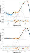 |
Fig. 1. Spectral energy distributions for two sources: G159.02-33.88 (top) and G195.90-02.60 (bottom). In each panel, the solid black line shows the best-fit model, with χred2 = 0.8 and 0.7, respectively. Individual realizations from the converged MCMC chain, illustrating model scatter, are shown in blue. Color-corrected flux densities are plotted as orange points, with hollow markers indicating data points excluded from the fit due to residual CO contamination or excessively high frequencies. Each individual best-fit model component is displayed in gray, with the dotted line representing the AME component. The lower sub-panels display residuals in units of statistical deviation from the fit, with the 1σ region shaded in light blue. |
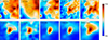 |
Fig. 2. Morphology of high-latitude source G159.02-33.88 in selected maps consisting of a collection of dark clouds, including LDN 1454/53/58 and DOBASHI 4162. The solid circle (72′ radius) marks the primary aperture, while the dashed annulus (96′–120′) represents the background region. The grid spans 6.7° per side. The AME component is visible above 5 GHz, with a strong correspondence between the WMAP K-band (22.8 GHz) near the AME peak and the DIRBE 240 μm (1249 GHz) map near the thermal dust peak. The reprocessed WISE 12 μm PAH-dominated map from Meisner & Finkbeiner (2014) is also shown. The color scale is linear and has been normalized to the pixel range of each image. |
For comparison, the bottom panel of Fig. 1 shows the SED of G195.90-02.60, a high signal-to-noise source near the Galactic plane that includes LDN 1591, LDN 1592, and LDN 1593. Its AME level is similar at ≈5 Jy, but the free–free emission is roughly 50 times brighter.
4. Results and discussion
4.1. Sky distribution and source selection
The sky distribution of the sources analyzed in this work is shown in Fig. 3 against a background of thermal dust emission as seen by the DIRBE 240 μm band. Their properties and physical natures are listed in Table A.1. Most sources are concentrated along the Galactic plane, while a significant number trace thermal dust features at mid-latitudes; 40% of sources are located at latitudes |b|> 10°, with approximately 20% of these having latitudes greater than 20°.
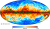 |
Fig. 3. Locations of the 144 AME sources with > 2σ detection, represented by green stars, on top of the DIRBE 240 μm map. |
The sample includes 57 sources from Planck Collaboration XV (2014) and 4 unique sources from Poidevin et al. (2023). The remaining 83 new sources are identified through visual inspection of an updated reduction of the Planck Collaboration X (2016) foreground model, derived using spectral parametric fitting with the COMMANDER component separation code (Eriksen et al. 2008). This reduction incorporates C-BASS and S-PASS data, enabling a more reliable extraction of the AME amplitude (Hoerning et al., in prep.). The AME amplitude map is compared to the Planck 857 GHz emission at 1° scales, and compact sources appearing in both maps are manually selected. Each source is then cross-checked in the SIMBAD9 database to confirm its Galactic origin and to characterize its nature and physical environment. Additionally, sources are verified against the Radio Fundamental Catalog (Petrov & Kovalev 2025) to exclude those with significant quasar or blazar contamination (> 0.5 Jy) in the primary or background apertures.
The use of the Hoerning et al. (in prep.) map is not essential for reproducing our source selection. A similar source list could be obtained through alternative methods, such as identifying clumps directly or extrapolating free–free emission from C-BASS maps to 22.8 GHz and subtracting this estimate from WMAP K-band at the same frequency, though at significantly greater effort. However, our criterion of selecting AME sources only when they have a thermal dust emission counterpart inherently biases against any potential AME sources arising from a dust-independent emission mechanism.
Almost every source contains a mixture of dark and molecular clouds along with associated H II regions. However, for some extended sources at high latitudes, molecular cloud and dark cloud catalogs are unavailable, with exceptions for well-known sources (e.g., ρ Ophiuchi). For these high-latitude extended sources, the primary references are IRAS FIR sources (Helou & Walker 1988) and Planck Galactic Cold Clumps (Planck Collaboration XXVIII 2016), which often encompass multiple individual dark and molecular clouds.
Most sources are compact relative to a 1° beam, with 74% having a primary aperture radius of 1° and 24% ranging from 1.0° to 1.5°. Only three sources exceed this size, the largest being G170.60-37.30 (the translucent molecular cloud MBM16) with a radius of 2.5°. The sample has a mean radius of 1.1°, with a standard deviation of 0.2°. While these sources are not strictly compact in a morphological sense, their emission typically manifests as a single, centrally peaked structure without pronounced substructure, with the signal largely contained within a 2° aperture; for an illustrative example, see Fig. 2.
The selection criteria can introduce biases in the observed AME population, and as a result, we do not present a complete catalog–this is not the objective of our study. To be included in this analysis, sources must have a well-determined peak frequency and width, with AME detected at a significance level greater than 2σ. Among the 144 sources that meet these criteria, 10 have significances in the 2–3σ range; the rest are > 3σ. For comparison, Planck Collaboration XV (2014) reported 42 significant AME sources out of 98, and Poidevin et al. (2023) found 44 out of 52. Our sample increases the number of significant sources by a factor of 3.3, with amplitude, peak frequency, and width constrained for each. However, in the southern hemisphere, the lack of QUIJOTE data limits width constraints, reducing the number of identified sources there. As a result, southern hemisphere sources tend to be the brightest, with the highest AME-to-free–free contrast. This strict requirement for fully constrained amplitudes, peak frequencies, and widths excludes many sources with potentially significant AME, particularly those with lower AME contrast for which the width cannot be well constrained.
A significant fraction of AME in the sky is diffuse on scales of several degrees or more, but our use of aperture photometry restricts the analysis to relatively compact sources (≈1°) that are substantially brighter than their surroundings. In some mid-latitude clouds, AME is so diffuse at 1° scales that it becomes undetectable by aperture photometry techniques. Nevertheless, aperture photometry provides the advantage of isolating emission from individual physical sources rather than capturing the total emission along a given line of sight, as is the case in studies such as Fernández-Torreiro et al. (2023). At high Galactic latitudes, detecting AME is particularly challenging because the background fluctuations within the aperture are often comparable to the source emission itself. This reduces the effective signal-to-noise ratio and can bias the derived spectrum if the background has a different spectral shape than the source. As a result, high-latitude detections are limited to sources with strong emission relative to the local background variations.
Another selection bias stems from the noise-limited sensitivity of the data, which prevents the detection of AME sources significantly fainter than ≲1 Jy. Since the power emitted by spinning dust grains scales with the fourth power of their rotational speed, this sensitivity limit effectively imposes a constraint on peak frequency–sources with very low peak frequencies become too faint to detect below a certain threshold. This is supported by our ability to probe lower frequencies compared to previous studies due to improved low-frequency data (see Sect. 4.3.4).
Additionally, in bright regions dominated by calibration uncertainties, the relative contrast between AME and free–free emission introduces an additional limitation. If AME is brighter than free–free emission by an amount comparable to the calibration errors of low-frequency surveys (e.g., ∼5%), it cannot be reliably detected. This bias favors sources with a higher contrast of AME relative to free–free emission. In fact, the minimum ratio of AME to total emission at the peak frequency for our sample is ≈12%, consistent with the calibration uncertainties of the low-frequency data and AME significance levels of the sample.
Achieving completeness in flux density is only possible at the very brightest levels, given the combination of systematics and background complexity. Furthermore, completeness in luminosity, which would reflect the intrinsic emission of each source, is infeasible because of uncertain distances. Given these limitations, our sample is predominantly composed of compact sources with good data coverage, high contrast against free–free emission, and sufficient brightness to be detected above noise thresholds. As a result, the AME catalog presented in this paper is not complete to a well-defined flux-density threshold, although as a reference, the faintest AME detections in the sample are at the ≈0.7 Jy level. Nevertheless, it represents the largest and most accurate set of AME detections and spectra to date, providing a robust basis for sub-sample analyses and tests of selection biases.
4.2. AME parameters
4.2.1. Parameter distributions
Figure 4 shows the distributions of the fit AME parameters: amplitude, peak frequency, and width. The left panel shows the AME amplitude distribution, which has a median value of 5.2 Jy and a median uncertainty of 0.6 Jy. These values translate to a median AME detection significance of AAME/σAAME ≈ 7σ and a minimum significance of ≈2σ. The ratios of AME to total emission at the peak frequency range from 12% to nearly 100%, with a median AME fraction of 64% at the peak frequency.
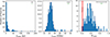 |
Fig. 4. Distributions of AME parameters in the source sample. Each panel includes an inset in the top-right showing the median (black) and smallest (green) 1σ uncertainties for that parameter among all sources. For AAME, the median and smallest uncertainties are 0.6 Jy and 0.1 Jy, respectively; the corresponding uncertainty bars are not visually discernible, as their horizontal caps are unresolved at the adopted linewidth. A best-fit Gaussian is drawn as a dashed red line on the νAME and WAME distributions. The red shaded region in the WAME panel highlights the range of effective widths predicted by single-phase SPDUST2 and SPYDUST templates (see Table 2). |
The central panel presents the distribution of AME peak frequencies, predominantly between 10 and 35 GHz. Few sources show peak frequencies above 35 GHz, and these have relatively large uncertainties. The highest peak frequency in our sample is νAME = 62 ± 13 GHz for the California Nebula, consistent with the Planck Collaboration XV (2014) value of 50 ± 17 GHz. The slightly smaller uncertainty arises from improved modeling of the low-frequency components, since the AME peak itself remains constrained entirely by WMAP/Planck data. The median νAME is 22.4 GHz, with a median uncertainty of 1.9 GHz. The distribution approximates a normal distribution with a mean of 21.9 GHz and standard deviation of 3.7 GHz (red-dashed line). However, this Gaussian shape likely results from the central limit theorem rather than being an intrinsic property, as detection bias exists against very low peak-frequency sources (see Sect. 4.1). This bias is evident in previous studies, which lacked detections below ∼17 GHz due to fewer low-frequency datasets. Notably, no sources peak at the very high frequencies predicted by theoretical models for reflection nebulae and photodissociation regions, which the current data and source selection criteria would be sensitive to, at least at the low-frequency end (< 100 GHz) not embedded in thermal dust emission.
The peak frequency as a function of absolute latitude exhibits a small but statistically significant downward trend when fit linearly, with higher-latitude sources tending to have lower peak frequencies. The best-fit line intercepts the Galactic plane at 23.7 ± 0.6 GHz with a slope of −0.076 ± 0.034 GHz deg−1 (2.2σ). This pattern parallels the general decrease in dust temperature at higher latitudes seen in our sample. The substantial scatter and high χred2 = 9.8 suggest that local environmental factors strongly influence individual source peak frequencies, making latitude alone an inadequate predictor.
The right panel illustrates the distribution of the width parameter. The median width is 0.57, with a standard deviation of 0.10 and a median uncertainty of 0.11 for any given source. We find no significant correlation between width and latitude, given that the uncertainties are large compared to the overall variation across the sample, although narrower widths generally have smaller associated uncertainties. Crucially, no source has a width narrower than the theoretical effective widths predicted by single-component SPDUST2 or SPYDUST models (red shaded region), and the observed distribution is generally much broader than these expectations. This result, consistent with findings for diffuse emission in the Galactic plane (Fernández-Torreiro et al. 2023) and in λ Orionis (Cepeda-Arroita et al. 2021), is a major conclusion of this analysis, and strongly indicates that single interstellar medium (ISM) phase spinning dust models cannot generally capture the observed AME width. Such broadness motivated the use of a two-component model in Planck Collaboration XXV (2016)–with one fixed high-frequency and one varying low-frequency component–which better fit the then-limited data. It is now clear that this broadness is a prevalent feature, which we interpret as evidence of multiple spinning dust components within most compact sources or along most lines of sight, possibly also reflecting the fact that current theoretical models might not capture the full range of grain sizes encountered in the ISM, which would broaden the spectrum. Furthermore, widths narrower than 0.4 would have been observed if they existed, given that neither the sample selection nor fitting methodology is biased against narrower sources. The fact that theoretical predictions accurately reproduce the minimum observed width provides important new support for the spinning dust hypothesis.
Based on the observed distributions of peak frequencies and widths, a rough Gaussian approximation, νAME ∼ 𝒩(21.9, 3.7 GHz) and WAME ∼ 𝒩(0.56, 0.10), may serve as a practical starting point for defining informative priors in studies that lack direct constraints on these parameters, as shown by the red-dashed lines in Fig. 4. The derived distributions closely match those in Fernández-Torreiro et al. (2023), suggesting broader applicability in diffuse regions. However, potential biases in our sample should be considered, such as reduced sensitivity to low νAME values and the prior’s inability to accommodate high-frequency sources such as the California nebula. These priors should therefore be used with caution.
The thermal dust emission (not shown) shows temperatures in the range 14 < Td < 28 K, with a median of 19.0 K and median uncertainty of 0.7 K. The dust emissivity index is in the range 1.2 < βd < 2.2, with a median of 1.6 and typical uncertainty of 0.09, consistent with values found by Planck Collaboration XI (2014) over the full sky. The median value of the synchrotron spectral index for sources including this component is −1.1, consistent with expectations.
4.2.2. Impact of low-frequency data: Comparison to previous AME studies
We compared our best-fit parameters with those from previous studies for sources in common. We focused on AME amplitude and peak frequency (see Fig. 5).
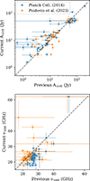 |
Fig. 5. Comparison of this work (y-axis) with previous studies (x-axis) for AAME (top panel) and νAME (bottom panel). The dashed gray line represents a 1:1 relation. |
Our free–free emission estimates align well with previous studies, with uncertainties in EM about two-thirds those of Planck Collaboration XV (2014). However, Poidevin et al. (2023) reports EM uncertainties nearly half of ours, likely due to their assumption of 10% effective calibration uncertainties for the lowest-frequency surveys. These surveys suffer from variable, scale-dependent calibration factors (see Sect. 2.4). The absence of C-BASS and S-PASS data in Poidevin et al. (2023) implies that the uncertainties in free–free and synchrotron emission may have been underestimated, potentially resulting in artificial high-significance AME detections in some sources.
The AME amplitudes (top panel) are generally consistent with Planck Collaboration XV (2014), with a systematic underestimation for sources in the 5–10 Jy range relative to our results. Compared to Poidevin et al. (2023), our results show less scatter, but some amplitudes are inconsistent, likely due to underestimated calibration uncertainties at low frequencies and least-squares fitting used in Poidevin et al. (2023) falling into local minima. In fact, AME significances in our study align better with those from Planck Collaboration XV (2014). The uncertainties in AAME are, on average, 10% smaller than Poidevin et al. (2023) and 30% smaller than Planck Collaboration XV (2014) for common sources thanks to additional data in the range 2.3–19 GHz.
The bottom panel compares peak frequencies. Planck Collaboration XV (2014) exhibits a systematic bias toward higher peak frequencies, predominantly falling to the right of the 1:1 line. A best-fit scaling factor of 0.87 ± 0.02 implies a peak frequency bias of −13 ± 2% on average–substantially larger than the expected ≈ − 6% bias from modeling a theoretical template with a log-Gaussian function. We attribute the larger bias to the limited low-frequency data in Planck Collaboration XV (2014), which tends to push peak frequencies higher, especially in cases where data do not cover both sides of the peak, as clearly demonstrated in Rennie et al. (2022). In addition, fixing the width to that of a theoretical template when the real widths are generally broader might also have biased the peak frequency. In contrast, Poidevin et al. (2023) shows a scaling factor of 1.04 ± 0.04, indicating consistency. Our peak frequency uncertainties are, on average, 2.7 times smaller than those in Poidevin et al. (2023).
In H II regions such as the Rosette Nebula, where AME has very low contrast, the absence of QUIJOTE data leaves its width unconstrained and often biases it toward higher values. For this reason, the Rosette Nebula is not included in the catalog. This highlights the necessity of QUIJOTE observations in low AME contrast sources for fully constraining all AME parameters. More broadly, our comparison emphasizes the critical role of data below 20 GHz in accurately determining AME amplitude, frequency and width. Combining low-frequency datasets such as C-BASS and S-PASS to establish a reliable baseline for free–free and synchrotron emission–alongside QUIJOTE–remains essential for robust peak frequency measurements.
4.2.3. Systematic deviations from the fit model and calibration systematics
We assessed potential miscalibration and foreground mismodeling by examining systematic deviations of flux densities from the best-fit SED models. This involves computing the ratio of best-fit to measured flux density at each frequency and deriving a weighted mean to quantify any systematic offset. Our analysis focuses on point-like sources that fit within 1°-radius primary apertures, effectively excluding extended sources in order to assess calibration systematics.
Most datasets show good agreement with the best-fit models, including C-BASS and the 1420 MHz Stockert/Villa-Elisa survey (Reich et al. 2001). Our independent derivation of the point-source calibration factor is 1.57 ± 0.06, consistent with the 1.55 ± 0.08 reported by Reich & Reich (1988) and applied in this study. Our factor is confirmed through a second iteration of the SED fits in which the data point is already corrected by the original Reich & Reich (1988) factor, implying convergence. We find no significant latitude dependence, though uncertainties remain large for high-latitude bins due to the lower number of sources.
However, the S-PASS dataset systematically exceeds the model fit by a factor of 1.10 ± 0.02, while the HartRAO survey appears slightly low at 0.97 ± 0.02. A direct T-T plot comparison between the HartRAO 2.303 GHz survey and S-PASS confirms that S-PASS is higher by a factor of 1.195 ± 0.003. Since we weight S-PASS more strongly than HartRAO in the fit and the two datasets frequently overlap, the higher discrepancy between the two datasets aligns with the deviations observed with respect to the line of best fit. Further validation comes from source W37, which lies in a region covered by S-PASS, HartRAO, C-BASS, and QUIJOTE. There, the S-PASS flux density is ∼13% above the best-fit line, significantly larger than the quoted calibration uncertainty of 5%. This potential miscalibration could lead to slightly inflated estimates of free–free emission in the Southern Hemisphere, reducing AME detections and biasing the sample toward regions with high AME to free–free contrast.
A likely reason for the overcalibration of S-PASS is sidelobe integration when smoothing to 1° FWHM from its native 8.9 arcmin resolution. The Parkes telescope’s main beam efficiency is approximately 63% at the L-band (Barnes et al. 2001), and while it has not been publicly reported at the S-band, it is expected to be similar. Carretti et al. (2019) do not perform detailed beam modeling or give an explicit value. Proper beam characterization and deconvolution are therefore crucial for fully leveraging S-PASS data in spinning dust studies, particularly for AME analysis in future COMMANDER runs. Similar overcalibration effects are also likely to impact polarized synchrotron studies at 1° FWHM.
The QUIJOTE MFI datasets exhibit a small but measurable trend relative to the line of best fit: the 11 GHz band is slightly low at 0.972 ± 0.009, the 13 GHz band is consistent with the fit, and the higher two bands are slightly high at 1.035 ± 0.009. Since this trend runs counter to the excess flux expected from modeling spinning dust spectra with a log-Gaussian distribution (see Sect. 4.3.6), it likely originates from excess atmospheric emission stripes, particularly at the higher 17 and 19 GHz bands for high latitude and therefore lower signal-to-noise sources. These deviations are consistent with those found in Rubiño-Martín et al. (2023) through CMB cross-correlations and remain within the quoted 5% uncertainty.
4.3. Spectral variations and the nature of AME
4.3.1. Correlation analysis and methodological limitations
Spearman’s rank correlation coefficients, rs, are a powerful tool for assessing monotonic but not necessarily linear relationships between parameters (Spearman 1904). We compute rs for every parameter combination across all datasets described in Sect. 4.3.2, using the spearmanr function from SCIPY (Virtanen et al. 2020). These correlations are robust to offsets and miscalibration, making them effective for identifying phenomenological trends when the underlying physical relationship is unknown.
However, Spearman correlation relies on rank ordering, and any noise that disrupts this ordering can reduce the measured rs relative to the underlying true correlation. It may also fail to capture strong but non-monotonic relationships, such as those involving inflection points or more complex structures. Importantly, a high degree of correlation does not imply causation. Apparent correlations may arise from a shared dependence on a third variable or additional variables, while weak correlations may be statistically insignificant or spurious. Source selection for incomplete samples and fitting biases must also be considered.
In pairwise correlations, multidimensional relationships between variables may be obscured by confounding variables. As an analogy, a dataset describing the speed and mass of objects in relation to their kinetic energy will only show a tight pairwise correlation when one of the two variables is held relatively constant. Similarly, AME observables may depend on several environmental parameters simultaneously, so two-variable correlations alone may be inconclusive. This motivates the use of multivariate approaches, particularly machine learning methods. Random Forests (Breiman 2001), for instance, can rank the relative importance of each parameter in predicting a given AME observable, highlighting the dominant physical processes at play. Symbolic Regression techniques, often based on genetic algorithms, extend this by producing compact analytical expressions that balance predictive power with interpretability. Sparse methods such as SINDY (Brunton et al. 2016) assume that only a few terms govern most systems and have been successful in rediscovering known laws in complex regimes such as fluid dynamics. Similarly, multivariate adaptive regression splines (Friedman 1991) model nonlinearities with piecewise linear fits, yielding explicit equations with clear interpretability. The exploration of multivariate AME correlations using these techniques is suggested as a future extension to this work.
To estimate the impact of observational uncertainties on rs, we perform a Monte Carlo randomization of each data point based on its Markov chain, neglecting systematic calibration errors and assuming Gaussian uncertainties for photometric data. We also verify that sources with and without QUIJOTE data follow consistent distributions, confirming the absence of spectral coverage bias. This is expected for the relatively high signal-to-noise sources studied in the Southern sky.
4.3.2. AME observables and environmental tracers
The fit SEDs provide three key AME observables: the AME amplitude, the peak frequency, and the spectral width, with no significant correlations observed between them. The peak frequency and spectral width emerge as properties of the underlying dust grain population, while the amplitude must be normalized to derive a physically meaningful emissivity.
To quantify the AME emissivity, we adopt three normalization schemes for the fit amplitude AAME. The first and most common approach is to normalize by the product of the dust optical depth at 353 GHz, τ353, and the solid angle of the primary aperture, Ω, using AAME/(τ353 ⋅ Ω). This method accounts for variations in source size across different regions. Although this normalization is standard, it introduces some scatter since the true source size is unknown and the aperture area is only an approximation.
The use of τ353 is motivated by the fact that it traces the dust column density and, under the assumption of a relatively constant dust-to-gas ratio, is often used as a proxy for the total hydrogen column density (Planck Collaboration XIX 2011). This allows, in principle, for direct comparison with theoretical models of spinning dust emission by converting the measured AME emissivity into a per-hydrogen-atom basis. However, this assumption is only approximate: the τ353–NH relation is known to vary by at least a factor of ∼2 (Planck Collaboration XI 2014), and potentially more at low Galactic latitudes where dust properties and radiation fields are more complex.
Furthermore, variations in density within an aperture introduce additional scatter: dense clumps may occupy only a small fraction of the beam, biasing the effective τ353 estimate when averaging over the entire region. Most critically, AME is thought to arise from very small grains or PAHs, whereas the total dust mass (and thus τ353) is dominated by large grains. This mismatch means that τ353 may not be an optimal tracer of the relevant grain population, particularly in regions where environmental conditions strongly affect the abundance of small grains.
As an alternative, we normalized the AME amplitude using the dust radiance, defined as
 (12)
(12)
where Sd(ν) is the spectral energy distribution of the thermal dust emission. We also computed the AME radiance, ℜAME, in an analogous way and normalized it by ℜd to express the AME flux relative to the total thermal dust emission. This provides a direct comparison between the energy budgets of the two mechanisms.
Environmental parameters considered in our analysis include the dust temperature, optical depth, and emissivity index, as well as the emission measure of free–free emission. For a subset of sources, synchrotron parameters are also included. In addition to these, we derived composite quantities such as the peak frequency and flux density of the thermal dust emission, the dust and AME radiances, and a tracer of the interstellar radiation field strength following Mathis et al. (1983):
 (13)
(13)
Although G0 is a widely used tracer of the interstellar radiation field, it assumes the average values produced by local stars in the diffuse ISM. It does not account for the specific stellar population or radiation field shape in each individual region, which can vary significantly. This makes G0 a reasonable approximation at high Galactic latitudes, but at low latitudes greater scatter is expected.
To investigate the link between PAHs and AME, we used the reprocessed WISE 12 μm map from Meisner & Finkbeiner (2014), which removes instrumental artifacts and continuum starlight. Within this bandpass, PAH molecules are believed to dominate the emission, although their abundance and spectral features vary considerably across regions (Boersma et al. 2010). Following the method of Hensley et al. (2016), we construct a tracer for the fractional PAH abundance by dividing photometry of the 12 μm map by the dust radiance.
4.3.3. AME tracers
We analyzed the correlations between AME amplitude and various environmental parameters to identify the most effective predictor of AME at 1° scales. Figure 6 highlights the relationships between AME amplitude and both dust optical depth (τ353) and dust radiance (ℜd). We also correlated AME amplitude with the flux density from each frequency map in Table 1, following Cepeda-Arroita et al. (2021), with results for datasets above 20 GHz shown in Fig. 7.
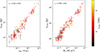 |
Fig. 6. Anomalous Microwave Emission amplitude correlations against τ353 ⋅ Ω (left), where Ω is the primary aperture solid angle, and dust radiance ℜd (right). The points are color coded by peak frequency, with sources above 35 GHz truncated to the upper color limit. Best-fit models are shown by gray dashed lines: linear for the optical depth correlation (left) and power-law for the dust radiance correlation (right). |
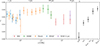 |
Fig. 7. Spearman correlation coefficients between AAME and individual frequency maps. Tracers are shown on the right, where CO denotes the 1–0 CO transition map by Ghosh et al. (2024) and Speak, d is the flux density at the peak of the thermal dust emission fit. In both cases, τ353 refers to the angular area-corrected optical depth τ353 ⋅ Ω. Hollow points denote frequencies that are excluded from the SED fitting. The 100 and 217 GHz bands are CO-subtracted. |
We found a strong correlation between AME amplitude and thermal dust emission. We specifically highlight the relationships with optical depth τ353 and dust radiance. These correlations, previously reported in the literature, are now extended by our high-latitude sources to include fainter AME detections. Dust radiance exhibits a tighter correlation with AME amplitude than optical depth, suggesting it is a more effective tracer.
Fitting the AAME–τ353 ⋅ Ω relation with a power law using orthogonal distance regression (Boggs & Rogers 1990) yielded an exponent of 0.99 ± 0.03, which is consistent with linearity. A linear fit returns an intercept of 0.25 ± 0.18 Jy, which is marginally consistent with zero. The scatter is approximately 50%, with an orthogonal χred2 ≈ 12, even when forcing the fit through the origin (see Fig. 6). The best-fit relation is
 (14)
(14)
The high χred2 reflects intrinsic environmental variations between regions, leading to ≈50% deviations from this linear prediction. A linear relationship is expected physically, as AAME scales with column density of small grains, which are usually well-mixed with the larger grains traced by τ353. No significant dependence on peak frequency is observed in this correlation. For the typical νAME ∼ 22 GHz, the scaling yields an AME amplitude of ∼16 K per τ353, although this value should be regarded as indicative only, given the angular dilution inherent in Ω.
The AAME–ℜd relation follows a power law:
 (15)
(15)
This fit exhibits a reduced scatter of 33%, indicating that ℜd is a more precise predictor than τ353. However, the still-elevated χred2 ≈ 3 suggests intrinsic source-to-source variability. A mild excess in dust radiance is observed around AAME ≈ 10 Jy, coinciding with sources that exhibit higher peak frequencies.
The improved correlation of ℜd over τ353 aligns with earlier findings (Hensley et al. 2016; Cepeda-Arroita et al. 2021; Poidevin et al. 2023; Fernández-Torreiro et al. 2023). Several factors likely contribute to this: (1) τ353 is more model-dependent than ℜd, which can be directly calculated by integration with minimal modeling; (2) the use of primary aperture area as a proxy for source size introduces scatter, especially for more extended, lower-AME sources; and (3) τ353 primarily traces large grains, whereas AME arises from very small grains–so variations in the ratio of large-to-small grains introduces additional scatter. A more in-depth discussion of small grain tracers, including PAHs, is provided in Sect. 4.3.5.
A similarly tight correlation exists between AME amplitude and the peak flux of thermal dust emission:
 (16)
(16)
This relation has a typical scatter of 32% and a Spearman coefficient comparable to that of ℜd. The corresponding AME emissivity, AAME/Sd, peak, decreases with source brightness, ranging from ∼0.04% for the faintest sources to ∼0.009% for the brightest, changing by a factor of ≈5 across our sample.
We also compared the total radiative energy outputs:
 (17)
(17)
This relation yields rs = 0.94 ± 0.03 and a scatter of 52%, likely due to larger uncertainties in deriving AME radiance. The corresponding AME radiative emissivity, ℜAME/ℜd, decreases with increasing source radiance, ranging from ∼3 ⋅ 10−6 for the faintest sources to ∼1 ⋅ 10−6 for the brightest, changing by a factor of ≈3 across our sample.
A commonly used historical measure of AME emissivity is the ratio of the AME residual flux density at 28.4 GHz to the 100 μm flux density. In our sample, this ratio decreases from ∼9 ⋅ 10−4 for the faintest thermal dust emission sources to ∼1 ⋅ 10−4 for the brightest, a variation of nearly an order of magnitude. The median value, 3.7 ⋅ 10−4, is similar to the values found in Planck Collaboration XV (2014). The ratio follows an approximate power-law dependence on the 100 μm flux density, scaling as  , indicating that a single average ratio poorly represents the sample. This trend mirrors the sublinear behavior of AME amplitude and radiance with respect to thermal dust emission. However, this emissivity definition is problematic because it relies on fixed reference frequencies that are highly sensitive to both the AME peak frequency and the thermal dust temperature, as evidenced by its large scatter. Peak amplitude ratios should therefore be used as a more fundamental and consistent basis for defining AME emissivities.
All in all, the sublinear indices for both AME amplitude and radiance indicate that AME increases more slowly than thermal dust emission. This suggests that brighter dust environments are less efficient at producing spinning dust emission. One possible cause is photodissociation of small grains in strong radiation fields, but if that were dominant, we would expect the brightest sources to have systematically hotter dust. We do not observe a clear trend, suggesting that photodissociation may not be the primary mechanism. A more likely explanation is grain evolution in dense, shielded environments, where the smallest grains may coagulate onto larger grains and be effectively depleted. Compiègne et al. (2008) show that in photodissociation regions the ratio of PAH to small-grain abundance declines by factors of 2–5 in dense zones compared to diffuse regions, while Arab et al. (2012) find strong PAH depletion in the Orion Bar consistent with coagulation processes. These results support the idea that small-grain depletion suppresses AME relative to thermal dust emission in denser dust environments.
Figure 7 shows the frequency-dependent correlations of AME amplitude with individual maps. The strongest correlation occurs at DIRBE 240 μm (∼1.3 THz), near the peak of thermal dust emission for our sample, 1.8 ± 0.2 THz. A secondary maximum appears at ∼20 GHz, consistent with the AME peak. Correlations decline at CMB-dominated frequencies due to reduced AME contribution and lower signal-to-noise. The QUIJOTE frequencies, not shown, display reduced correlation coefficients due to lower signal-to-noise, precluding direct comparison with WMAP. The impact of noise is also evident in the Planck 100 GHz map, where the correlation is reduced due to scatter introduced by the CO correction.
Following the peak near the thermal dust maximum, the correlation coefficient declines steadily, reaching a minimum at the IRIS 60 μm band before rising again–an effect previously reported by Fernández-Torreiro et al. (2023), Cepeda-Arroita et al. (2021), Bell et al. (2019). As thermal dust emission from large grains decreases above ≈2 THz, the contribution from stochastically heated very small grains (VSGs), which are not in thermal equilibrium, becomes increasingly significant, particularly above ≈3 THz (100 μm). This emission component typically dominates around the 60 μm band, where the observed correlation with AME is lowest (Compiègne et al. 2011). The dip in correlation between the thermal dust peak and the WISE 12 μm band suggests that VSGs are not co-located with AME, whereas PAHs appear to be well mixed with spinning dust–at least at 1° resolution. The two points at 12 μm correspond to IRIS (red) and WISE (violet), with the reprocessed WISE 12 μm map (Meisner & Finkbeiner 2014) displaying a significantly better correlation due to the removal of continuum emission. However, due to noise biases in Spearman coefficients and systematics in the WISE 12 μm data, the lower correlation coefficient relative to the thermal dust peak cannot be taken as evidence against PAHs as the primary carriers of spinning dust. Rather, it supports the interpretation that PAHs are better co-located with AME than the transiently heated VSG population.
Correlation coefficients for several tracers are also displayed on the right of Fig. 7, with the correlation for the peak flux density of thermal dust emission being marginally better than ℜd, and comparable to the correlation coefficient of the DIRBE 240 μm band. In addition, a slightly stronger correlation is found through the product of τ353 with a tracer for the fraction of PAHs, fPAH, to be discussed in Sect. 4.3.5. The correlation coefficient with the dark gas map derived in Planck Collaboration XIX (2011, not shown) is 0.68 ± 0.09, though this is likely limited by systematics in its construction. In summary, the peak flux of thermal dust emission and dust radiance appear the best candidates for predicting the amplitude of AME at 1° scales, potentially accurate to within ≈30%.
4.3.4. Correlation between AME peak frequency and thermal dust temperature
The AME peak frequency is observed to positively correlate with the temperature of large dust grains, as shown in Fig. 8. This observed trend is not reproduced by current theoretical models. In nearly all the idealized environments listed in Table 2, increasing the temperature or radiation field over the ranges relevant to our sample leads to only negligible changes in the predicted AME peak frequency, as shown in Ali-Haïmoud et al. (2009) for a CNM template.
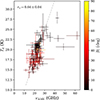 |
Fig. 8. Increase in AME peak frequency with thermal dust temperature. The color indicates the absolute Galactic latitude of each source. A linear best-fit model is shown in gray. |
Specifically, varying the dust temperature between 10 and 30 K produces nearly constant peak frequencies for most environments. Two notable exceptions are PDRs, which already predict very high peak frequencies (≳100 GHz), and dark clouds, which exhibit a quasi-logarithmic increase, with predicted peak frequencies rising from ∼29 to ∼37 GHz over the same temperature range. This trend is particularly relevant, as most of the sources in our sample are identified as containing dark clouds. This logarithmic behavior would manifest as an exponential function in Fig. 8; however, a linear fit provides a better match to the observed data, yielding χred2 ≈ 2.4, a typical scatter of 14%, and a slope of 1.35 ± 0.09 GHz K−1.
Similarly, increasing the radiation field intensity G0 while holding Td constant produces a significant increase in peak frequency only for dark cloud environments, with values rising from ∼30 to ∼80 GHz over the range of G0 of the sample. When both Td and G0 are increased simultaneously by coupling the variables through Eq. (13), the models predict a quasi-linear rise in the peak frequency from 30 to ∼80 GHz–about four times steeper per unit temperature than the trend observed in our data.
We interpret this disconnect between models and data as a consequence of the simplified treatment of environmental factors in theoretical frameworks, which employ fixed grain size distributions. The lack of dynamical modeling of how local conditions affect the grain size distribution likely prevents these models from capturing the full complexity of the phenomenon. In realistic environments, varying a single parameter–such as temperature or radiation field–cannot occur in isolation without also affecting other interrelated quantities such as density, grain size distribution, and dipole moments. This interdependence underscores the need to integrate dust evolution and radiative transfer processes into spinning dust models in a self-consistent way.
While it is conceivable that a multiparameter minimization algorithm–tuning three or four environmental variables simultaneously–could reproduce the observed trend, this approach would be computationally intensive and inefficient and would risk producing solutions that lack a solid physical basis. A more effective strategy is to aim to reproduce the observed correlation from first principles, guided by a more realistic and self-consistent treatment of environmental interactions.
Because the proxy used for G0 is closely derived from Td, the correlation between AME peak frequency and G0 yields a similarly strong coefficient and scatter. Nonetheless, we hypothesize that the observed phenomenological correlation is ultimately driven by the local radiation field, which both raises the dust temperature and produces more rapid spinning dust rotation through a reduction in grain sizes, increased collisions and stronger radiative torques.
Although our sample is biased against sources with very low νAME due to detectability limits, there is no comparable bias up to ∼100 GHz. At peak frequencies > 100 GHz, faint AME would be increasingly difficult to detect, as it becomes embedded within the thermal dust emission and is excluded by the limits we imposed on νAME to keep parameters physically reasonable. Nevertheless, the complete absence of peak frequencies near 100 GHz, expected in reflection nebulae and PDRs, indicates that they are intrinsically rare or suppressed rather than simply overlooked. A plausible explanation is reduced emissivity caused by photodissociation of small grains or rapid radiative energy loss from grains spinning at very high frequencies.
Four notable outliers with relatively large uncertainties in AME peak frequency are evident: the California Nebula (ℓ, b = 160.27, −12.36), with νAME = 62 ± 13 GHz; Sharpless 280 (208.80, −2.65), at 49 ± 9 GHz; W40 (28.79, +3.49), at 43 ± 5 GHz; and IC 410 (the Tadpole Nebula, 173.56, −1.76), at 42 ± 2 GHz. All are predominantly H II regions characterized by low AME contrast relative to the underlying free–free emission, contributing only 15–22% of the total flux density at the peak frequency. While similarly low AME fractions are observed in a few sources with peak frequencies between 20 and 35 GHz, none surpass 22% at higher frequencies. For comparison, the median AME fraction at peak in the full sample is 64%.
Importantly, these sources show significantly poorer fits when modeled with a purely free–free component, exhibiting clear residual bumps in the WMAP and Planck frequency bands–strongly indicating the presence of an AME component. The observed AME amplitudes are also well above the level of calibration systematics in the data, and the derived peak frequencies are largely insensitive to the choice of background subtraction aperture–further supporting their reliability. Their deviation from the main population may reflect intrinsically distinct physical conditions or environmental factors. Follow-up studies at higher angular resolution will be critical for probing the origin of their elevated peak frequencies and understanding the conditions that give rise to these outliers. Furthermore, if extremely high peak frequency (≳100 GHz) sources imply very low AME fractions (lower than ∼5%), calibration uncertainties in the current datasets would present a bias against their detection.
We also tested the analogy to Wien’s displacement law for thermal dust emission (i.e., νpeak, d ∝ Td1), which is effectively built into the parametric form of a modified-blackbody. By fitting Fig. 8 with a power law νAME ∝ Tdγ, we found a best-fit exponent of γ = 1.17 ± 0.08. Excluding the four outliers reduces this to γ = 1.10 ± 0.07, placing it marginally above unity. While this suggests that AME peak frequency increases more steeply with temperature than predicted by a direct Wien’s-law-like proportionality, the proximity of the exponent to 1 implies that the analogy may still be physically informative. However, we do not expect AME to strictly follow a Wien’s law relation. The grains responsible for thermal dust emission are not the same as those producing AME, and the fastest-spinning grains are likely in an out-of-thermal-equilibrium state due to rapid energy loss from radiative damping. The AME may originate from a “Goldilocks” region within the line of sight–where the local conditions favor efficient spinning dust emission–resulting in an effective temperature that differs from the beam-averaged Td. However, the fact that we see a relation implies that the local and beam-averaged Td must be linked at large scales.
Nevertheless, due to sample selection effects and low-νAME detection biases–as well as the presence of poorly understood outliers–this relation warrants reevaluation in a full-sky component-separated dataset where completeness can be better quantified. Overall, the positive correlation between AME peak frequency and thermal dust temperature likely reflects the influence of the radiation field on the grain size distribution–an interpretation that might explain prior observations (e.g., Arce-Tord et al. 2020; Cepeda-Arroita et al. 2021). The relatively tight relation observed for the majority of sources suggests that a fundamental, and potentially simple, physical mechanism governs the peak frequency of spinning dust, one that should eventually be reproduced by theoretical models that couple dust evolution, radiative transfer, and environmental conditions.
4.3.5. PAHs
Polycyclic aromatic hydrocarbons are planar organic molecules composed of multiple fused benzene rings, which are hexagonal and around 1 nm across. Their out-of-plane vibrational energy levels (bending modes) lead to distinct emission lines in the mid-IR (Tielens 2008). Their ubiquity and small size make them strong candidates for spinning dust emission. The smallest PAHs, such as naphthalene, have an effective rotational diameter of ≈0.72 nm and are believed to dominate the microwave emission, as they can reach the fastest rotational speeds and therefore radiate significant power. Nevertheless, in principle, any small, abundant molecule with a dipole moment could emit spinning dust radiation.
To investigate the link between PAHs and AME, we follow the methodology of Hensley et al. (2016) but take advantage of more accurate AME amplitude estimates enabled by new low-frequency data. As a tracer of PAH emission, we use the reprocessed WISE 12 μm map (Meisner & Finkbeiner 2014), which captures the strongest mid-infrared PAH features and is largely dominated by PAH emission. However, mid-IR observations at 12 μm are biased toward slightly larger PAHs than those thought to dominate spinning dust. Since rotational emission is highly sensitive to grain size, the smallest PAHs – only a few benzene rings in size – contribute disproportionately to the microwave signal, even if they represent only a minor fraction of the total PAH mass. Shorter-wavelength bands, such as DIRBE 3.5 μm, provide greater sensitivity to these smaller PAHs (Chuss et al. 2022), but suffer from low sensitivity and strong stellar contamination, making them difficult to use without heavy processing. We therefore implicitly make the assumption that large and small PAHs are spatially co-located. Very recently, Sponseller et al. (2025) reported PAH–AME correlations using the 3.3 μm maps, though their conclusions are limited by two systematics evident in regions such as λ Orionis (Cepeda-Arroita et al. 2021): (i) reliance on a parametric COMMANDER AME separation lacking low-frequency data, biased by up to a factor of ∼2, and (ii) possible stellar contamination, since many point sources visible at 3.3 μm are absent in the 12 μm AKARI data shown in Cepeda-Arroita et al. (2021). These challenges underscore why we adopt the reprocessed WISE 12 μm map as our main tracer, while highlighting the need for cleaner AME templates (Hoerning et al., in prep.) and future spectroscopy from SPHEREx (Crill et al. 2020) to robustly isolate PAH emission at 3.3 μm.
Unlike the full-sky pixel-based analysis in Hensley et al. (2016), we perform aperture photometry on individual sources, meaning that we cannot use the fine-grained mask used in their study. Instead, we manually mask nine prominent stripes caused by Moon contamination in the WISE 12 μm map, affecting ≈5% of the sky. We then perform photometry at 1° resolution on each source in our sample to obtain the 12 μm flux density, from which we derive a quantity proportional to the PAH fraction, fPAH ∝ S12 μm/ℜd, following Hensley et al. (2016). The dominance of PAHs in the reprocessed WISE 12 μm data is supported by the stronger correlation in Fig. 7 relative to the IRIS 12 μm map, which is not corrected for unrelated emission mechanisms.
Across our sample, this PAH fraction tracer varies by a factor of ∼6, implying that the fractional abundance of PAHs differs by less than an order of magnitude among the observed regions, as shown in Fig. 9. Despite the large uncertainties in deriving fPAH, a clear relationship with Td emerges in the left panel. The low Spearman rank correlation coefficient, consistent with zero, is unsurprising given the non-monotonic nature of the relationship, to which the Spearman statistic is largely insensitive. Notably, fPAH exhibits a peak around Td ∼ 18–20 K. The reduction in the fraction of PAHs at both high and low temperatures might be indicative of two physical processes: (1) At temperatures below 18 K, the decrease in the observed gas-phase PAH fraction might be attributable to the adsorption or freeze-out of PAH molecules onto the surfaces of the much larger cold dust grains in dense molecular clouds (Michoulier et al. 2018). This process depletes the population of free PAHs in the gas phase, inhibiting vibrational modes and therefore IR emission. (2) Conversely, at temperatures above this 20 K peak, the reduction in PAH fraction may be caused by the increased efficiency of PAH destruction through photodissociation by more intense UV radiation fields, which correlate with higher dust temperatures. Laboratory and modeling studies suggest that small PAHs are readily dissociated under such conditions, while larger PAHs are significantly more stable (e.g., Leger & Puget 1984; Montillaud et al. 2013). This parabolic behavior is not mirrored in the Td–ℜd relation, which shows a broadly positive trend with significant scatter, suggesting the observed maximum is not a sample-selection artifact.
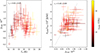 |
Fig. 9. Left: relation between the fraction of PAHs traced at 12 μm, fPAH, and thermal dust temperature, showing an inflection point. Right: AME emissivity relative to τ353 (a tracer of total column density) as a function of fPAH, with a linear best-fit model shown by the gray dashed line. The color encodes AME peak frequency. |
To examine the link between AME and PAHs, we compared the AME amplitude AAME against both τ353 and τ353 ⋅ fPAH, the latter serving as a proxy for the column density of PAHs. This connection was sought in Hensley et al. (2016), reporting a lack of correlation between AME and PAH emission and interpreting this as evidence against PAHs as AME carriers. However, their analysis also relied on AME amplitudes derived from the outdated Planck Collaboration X (2016) COMMANDER reduction, making the separation of AME from free–free emission highly degenerate. We argue that the lack of correlation in their study may be primarily driven by these systematics, which can easily mask underlying trends.
In our analysis, even though the product τ353 ⋅ fPAH introduces additional noise, we obtain a correlation coefficient of 0.933 ± 0.007–slightly higher (1.0 σ) than the 0.924 ± 0.006 found for τ353 alone, as seen in Fig. 7. The correlation also yields a best-fit power-law index of 1.02 ± 0.13, consistent with linearity. If fPAH were uncorrelated with AAME, introducing it should degrade the correlation. We test this by scrambling the fPAH values and repeating the analysis; the resulting correlations drop systematically to rs = 0.90 ± 0.01 on average, significantly (2.7σ) below the observed value. This is further supported by the direct correlation between fPAH and AME emissivity (Fig. 9, right panel), where a statistically significant positive trend is observed despite large scatter.
Taken together, these results provide circumstantial evidence of a connection between PAHs and AME, with spatial co-location at 1° scales. That said, our tracer is imperfect: the WISE 12 μm band suffers from systematic uncertainties and may include non-PAH contributions. Moreover, fPAH traces only the subset of PAHs emitting in the 12 μm band, whereas rotational emissivity is expected to depend sensitively on molecular size, charge state, and structure. Different PAH sub-populations (e.g., neutralversus ionized, small versus large) therefore contribute unequally to AME, but these cannot be disentangled with broadband WISE data. In addition, Hensley et al. (2022) argue that PAHs are systematically depleted in warmer gas, and that their IR emissivity per hydrogen atom varies with environment—possibly explaining why the mid-IR–AME correlation is weaker than expected. All of these effects would obscure the relation between PAHs and AME.
A definitive answer will require high-resolution spectroscopy to isolate PAH features from continuum and line emission mechanisms and to compare AME correlations against both PAH and thermal dust tracers. Such analyses would be particularly valuable at higher angular resolution, as the small spatial offsets seen at 1° between the PAH and AME (e.g., Fig. 2) could be amplified, enabling better identification of the specific carriers responsible for AME.
4.3.6. Systematic deviations from a log-Gaussian model
As noted in Sect. 3.2.3, the log-Gaussian approximation for the AME spectrum differs from physically motivated spinning dust templates. Consequently, if spinning dust emission is the true underlying process, we might expect systematic deviations of the photometry from the log-Gaussian best fit. To search for such deviations in the AME residuals, we use two approaches: (i) we normalize the photometric data relative to a single, standardized log-Gaussian function, and (ii) we examine the spectrum of the summed residual AME flux densities. The results of both methods are shown in Fig. 10.
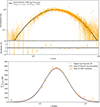 |
Fig. 10. Residuals of the fit data after subtracting all non-AME components. Top panel: residuals relative to a normalized log-Gaussian distribution. A transparency gradient was applied to deemphasize points with large error bars and enhance visual clarity. The lower sub-panel shows the binned weighted mean residuals as percentages relative to the standardized model, with bins evenly spaced in logarithmic scale. Bottom panel: total fit AME flux densities (orange) in a linear y-scale compared with the sum of best-fit log-Gaussian components (black). The sum only includes the 85 sources with simultaneous QUIJOTE and C-BASS coverage. A single log-Gaussian distribution fit to the AME residuals is shown as a dashed red line, with νAME = 22.8 GHz, WAME = 0.62 and χr2 = 3.1. |
To standardize the photometric data relative to a reference log-Gaussian model, we first subtract the best-fit contributions from other foreground components. The residual AME emission for each source is then rescaled linearly so that its log-Gaussian parameters match a common reference shape and normalization: we adopt an amplitude of Atarget = 1 Jy purely for convenience, along with a peak frequency νtarget = 22 GHz and a width Wtarget = 0.55. In this context, primed variables (ν′, S′) refer to the transformed quantities, while unprimed variables represent the original photometric measurements. The transformation of the frequencies is given by
 (18)
(18)
For flux densities, using the log-Gaussian function defined in Eq. (7), the transformation can be expressed as the ratio
 (19)
(19)
This scaling adjusts both the amplitude and shape of the distribution. Uncertainties in flux density are scaled by the same factor. This transformation enables direct comparison of the systematic deviations of the photometry from the fit model.
The standardized residuals (top panel of Fig. 10) display the normalized deviations for all sources. Given that most sources in our sample peak near ∼22 GHz, one might expect a consistent excess of flux below 10 GHz–corresponding to the slowly rising low-frequency tail of AME–if deviations from the log-Gaussian shape were present. However, this frequency range is poorly constrained due to the gap between C-BASS and the lowest QUIJOTE channel, which is visible in both figures.
Although the standardized log-Gaussian plot (top panel) displays a large number of points, only ≈13 photometric data points are fit per source. These are not independent across the sample, as they are all residuals relative to each source’s fit model. As such, the residuals are influenced both by observational systematics (e.g., calibration uncertainties) and by potential mismodeling of the AME spectrum, making it difficult to conclusively isolate intrinsic deviations from the log-Gaussian shape. Consequently, with such a limited number of points per source, the model can nearly always reproduce the data, potentially masking any underlying deviations. This is especially true in the 5–11 GHz range, where additional data near ≈7 GHz might be required to robustly identify low-frequency excesses.
The second approach examines the summed residual AME flux densities for the 85 sources with both C-BASS and QUIJOTE coverage (bottom panel of Fig. 10). Remarkably, the summed spectrum of fit AME components is well modeled by a single log-Gaussian function (red dashed line). This suggests that any individual source deviations from the log-Gaussian shape are either small relative to observational uncertainties or tend to average out across the sample, supporting the validity of the log-Gaussian parametrization as a reasonable empirical description of the ensemble AME behavior.
Both analyses reveal consistent features: a minor excess appears between 17 and 19 GHz with a corresponding deficit near 11 GHz. This feature aligns with the deviations discussed in Sect. 4.2.3, which we attribute to residual atmospheric signal in the higher QUIJOTE bands rather than intrinsic AME spectral deviations. A small excess is also seen just below 100 GHz, which might correspond to an unaccounted component or mismodeling of the foregrounds.
Overall, the analysis shows that the log-Gaussian model provides a remarkably good approximation across the available data, serving as a reasonable empirical description of the current datasets given their spectral coverage and systematics. To quantitatively assess whether theoretical spinning dust templates fit the data better, dedicated simulations would be required–particularly ones in which the width of the spinning dust spectrum is varied based on physical considerations, to reflect the broader distributions observed. We leave this as an illustrative case study of how such systematic deviations might be identified and interpreted in future work.
5. Conclusions
We have assembled the largest sample of compact AME sources to date, with AME amplitudes, peak frequencies, and widths derived with improved accuracy thanks to the merger of new low-frequency datasets, namely S-PASS, C-BASS, and QUIJOTE. We summarize this work with the following five key findings:
-
The observed widths of AME spectra are generally broader than those predicted by spinning dust models that assume a single ISM phase. This suggests contributions from multiple spinning dust phases within most of the sources studied or along the line of sight, and it may also reflect that theoretical models do not fully capture the range of grain sizes present in the ISM. The narrowest observed widths align with theoretical predictions for idealized templates, providing a new piece of evidence supporting the spinning dust hypothesis.
-
The AME amplitude is most effectively traced by thermal dust emission. Dust radiance and the peak flux of thermal dust exhibit the tightest correlations, with a typical scatter of around 30%, outperforming dust optical depth as predictors. The sublinear scaling of AME radiance with thermal dust radiance suggests that AME becomes less efficient in denser, more shielded environments, which is consistent with the depletion of small grains via coagulation onto larger ones.
-
We find a tight positive correlation between the AME peak frequency and the temperature of large dust grains, which current theoretical models fail to reproduce. The observed trend likely reflects the role of the local radiation field on grain properties, suggesting that spinning dust models must incorporate self-consistent radiative transfer and dust evolution treatment of the environmental parameters. Notably, we did not observe any sources with the extremely high peak frequencies expected for reflection nebulae and PDRs, suggesting the presence of a suppressive mechanism or an inherent detection bias, such as extremely low AME contrast or emissivity.
-
The PAH tracers exhibit characteristic environmental dependencies–likely driven by grain growth and photodissociation–and show a statistically significant but scattered correlation with AME emissivity. While systematic uncertainties in mid-IR tracers remain, our results support a physical connection between PAHs and AME, consistent with spatial co-location on degree scales.
-
The log-Gaussian model provides a good empirical approximation for the AME spectrum given the current spectral coverage and systematics of the available data.
This work highlights several directions for further study going forward. The relationships identified across our sample could inform improved Python Sky Model (Thorne et al. 2017) templates for spinning dust, particularly for better AME amplitude estimation, improving the separation of low-frequency components. Ongoing work (Hoerning et al., in prep.) and forthcoming 8–10 GHz observations from CGEM (Villalba-Gonzalez 2023) and improved 10–20 GHz observations with QUIJOTE MFI2 (Hoyland et al. 2022) will further refine these templates. To validate and extend these findings, a new COMMANDER component separation incorporating C-BASS, S-PASS, and QUIJOTE should be conducted to test the observed trends and improve sample completeness. The few sources with unusually high peak frequencies deserve detailed follow-up studies, as they may help isolate the physical conditions responsible for producing such high frequencies. More broadly, extending low-frequency datasets to full-sky coverage would be highly beneficial, particularly given that the absence of QUIJOTE coverage in the southern hemisphere visibly reduces detections in our study. Additionally, S-PASS would benefit from complete beam and sidelobe characterization, which is crucial for studying compact sources in both intensity and polarization at large angular scales. While we found no clear deviations from the log-Gaussian model, simulations could test whether current data are sensitive enough to detect asymmetries at lower frequencies and determine what level of systematic control would be required. Ultimately, establishing a definitive link between AME and specific molecules will require clean spectroscopic separation of PAHs and direct comparison with AME at finer angular scales. Upcoming SPHEREx all-sky survey data releases (Crill et al. 2020), which probe the 3.3 μm PAH feature, will be particularly valuable in this regard.
Finally, theoretical models must evolve to explain the trends we observed, including the broader spectral widths, the apparent absence of extremely high peak frequency sources, and the correlations with AME amplitude and peak frequency. This may require incorporating dynamical environmental conditions in spinning dust models. Data-driven tools such as symbolic regression could help uncover deeper multivariate patterns beyond simple pairwise correlations, providing insights that inform first-principles modeling.
Acknowledgments
The authors thank Jean-Philippe Bernard for providing the dark gas map used in the AME correlations, and Brandon Hensley for his insightful discussions and valuable input on theoretical aspects of this work. We also express our gratitude to David Chuss for organizing the “AME and its Connections to the Interstellar Medium” workshop at Villanova University, which greatly facilitated the exchange and development of ideas presented in this work, and for his helpful feedback on this paper. We further thank Alan Kogut and Ari Cukierman for useful discussions during the workshop. We also thank the anonymous referee for constructive comments that improved the clarity of this work. We thank the staff of the Teide Observatory for invaluable assistance in the commissioning and operation of QUIJOTE. The QUIJOTE experiment is being developed by the Instituto de Astrofisica de Canarias (IAC), the Instituto de Fisica de Cantabria (IFCA), and the Universities of Cantabria, Manchester and Cambridge. Partial financial support was provided by the Spanish Ministry of Science and Innovation under the projects AYA2007-68058-C03-01, AYA2007-68058-C03-02, AYA2010-21766-C03-01, AYA2010-21766-C03-02, AYA2014-60438-P, ESP2015-70646-C2-1-R, AYA2017-84185-P, ESP2017-83921-C2-1-R, PGC2018-101814-B-I00, PID2019-110610RB-C21, PID2020-120514GB-I00, IACA13-3E-2336, IACA15-BE-3707, EQC2018-004918-P, the Severo Ochoa Programs SEV-2015-0548 and CEX2019-000920-S, the Maria de Maeztu Program MDM-2017-0765, and by the Consolider-Ingenio project CSD2010-00064 (EPI: Exploring the Physics of Inflation). We acknowledge support from the ACIISI, Consejeria de Economia, Conocimiento y Empleo del Gobierno de Canarias and the European Regional Development Fund (ERDF) under grant with reference ProID2020010108, and Red de Investigación RED2022-134715-T funded by MCIN/AEI/10.13039/501100011033. This paper uses pre-publication data from the C-BASS project which is a collaboration between Oxford and Manchester Universities in the U.K., the California Institute of Technology in the U.S., Rhodes University, UKZN and the South African Radio Astronomy Observatory in South Africa, and the King Abdulaziz City for Science and Technology (KACST) in Saudi Arabia. The work at Oxford was supported by funding from STFC, the Royal Society and the University of Oxford. The work at the California Institute of Technology and Owens Valley Radio Observatory was supported by National Science Foundation (NSF) awards AST-0607857, AST-1010024, AST-1212217, and AST-1616227, and by NASA award NNX15AF06G. The work at Manchester was supported by several STFC Consolidated Grants and a UKSA grant (ST/Y005945/1) funding LiteBIRD foreground activities. A.C. Taylor and M.E. Jones also acknowledge support from the Horizon Europe Project RadioForegroundsPlus (GA 101135036) which is supported in the UK by UKRI grant number 10101603. This project has received funding from the Horizon Europe research and innovation program under GA 101135036 (RadioForegroundsPlus). CD and SEH acknowledge funding from an STFC (Consolidated Grant ST/P000649/1) and UKSA (LiteBird UK ST/Y005945/1). FP acknowledges support from the MICINN under grant number PID2022-141915NB-C21. DH acknowledges support from the MICINN under grant number PID2022-140670NA-I00. GAH acknowledges the funding from the Dean’s Doctoral Scholarship by the University of Manchester. MFT acknowledges support from the Enigmass+ research federation (CNRS, Universit Grenoble Alpes, Université Savoie Mont-Blanc). JC acknowledges support from the Fundación Occident and the Instituto de Astrofísica de Canarias under the Visiting Researcher Programme 2022-2025 agreed between both institutions. EMG acknowledges support from Plan Complementario AstroHEP funded by the “European Union NextGenerationEU/PRTR” and the Government of the Autonomous Community of Cantabria.
References
- Ali-Haïmoud, Y. 2010, Astrophysics Source Code Library [record ascl:10016] [Google Scholar]
- Ali-Haïmoud, Y., Hirata, C. M., & Dickinson, C. 2009, MNRAS, 395, 1055 [CrossRef] [Google Scholar]
- Alves, M. I. R., Davies, R. D., Dickinson, C., et al. 2012, MNRAS, 422, 2429 [NASA ADS] [CrossRef] [Google Scholar]
- Arab, H., Abergel, A., Habart, E., et al. 2012, A&A, 541, A19 [NASA ADS] [CrossRef] [EDP Sciences] [Google Scholar]
- Arce-Tord, C., Vidal, M., Casassus, S., et al. 2020, MNRAS, 495, 3482 [NASA ADS] [CrossRef] [Google Scholar]
- Armitage-Caplan, C., Dunkley, J., Eriksen, H. K., & Dickinson, C. 2012, MNRAS, 424, 1914 [NASA ADS] [CrossRef] [Google Scholar]
- Barnes, D. G., Staveley-Smith, L., de Blok, W. J. G., et al. 2001, MNRAS, 322, 486 [Google Scholar]
- Battistelli, E. S., Carretti, E., Cruciani, A., et al. 2015, ApJ, 801, 111 [Google Scholar]
- Battistelli, E. S., Fatigoni, S., Murgia, M., et al. 2019, ApJ, 877, L31 [Google Scholar]
- Bell, A. C., Onaka, T., Galliano, F., et al. 2019, PASJ, 71, 123 [NASA ADS] [Google Scholar]
- Bennett, C. L., Larson, D., Weiland, J. L., et al. 2013, ApJS, 208, 20 [Google Scholar]
- Boersma, C., Bauschlicher, C. W., Allamandola, L. J., et al. 2010, A&A, 511, A32 [NASA ADS] [CrossRef] [EDP Sciences] [Google Scholar]
- Boggs, P. T., & Rogers, J. E. 1990, Statistical Analysis of Measurement Error Models and Applications: Proceedings of the AMS-IMS-SIAM Joint Summer Research Conference held June 10-16, 1989, Contemporary Mathematics, 112 American Mathematical Society (AMS), 183 [Google Scholar]
- Breiman, L. 2001, Mach. Learn., 45, 5 [Google Scholar]
- Brunton, S. L., Proctor, J. L., & Kutz, J. N. 2016, Proc. Natl. Acad. Sci., 113, 3932 [Google Scholar]
- Cardoso, J. F., Martin, M., Delabrouille, J., Betoule, M., & Patanchon, G. 2008, ArXiv e-prints [arXiv:0803.1814] [Google Scholar]
- Carretti, E., Haverkorn, M., Staveley-Smith, L., et al. 2019, MNRAS, 489, 2330 [Google Scholar]
- Casassus, S., Dickinson, C., Cleary, K., et al. 2008, MNRAS, 391, 1075 [NASA ADS] [CrossRef] [Google Scholar]
- Cepeda-Arroita, R., Harper, S. E., Dickinson, C., et al. 2021, MNRAS, 503, 2927 [NASA ADS] [CrossRef] [Google Scholar]
- Chluba, J., Hill, J. C., & Abitbol, M. H. 2017, MNRAS, 472, 1195 [NASA ADS] [CrossRef] [Google Scholar]
- Chuss, D. T., Hensley, B. S., Kogut, A. J., et al. 2022, ApJ, 940, 59 [Google Scholar]
- Compiègne, M., Abergel, A., Verstraete, L., & Habart, E. 2008, A&A, 491, 797 [NASA ADS] [CrossRef] [EDP Sciences] [Google Scholar]
- Compiègne, M., Verstraete, L., Jones, A., et al. 2011, A&A, 525, A103 [Google Scholar]
- Crill, B. P., Werner, M., Akeson, R., et al. 2020, SPIE Conf. Ser., 11443, 114430I [Google Scholar]
- Dame, T. M., Hartmann, D., & Thaddeus, P. 2001, ApJ, 547, 792 [Google Scholar]
- de Oliveira-Costa, A. 1998, in Eighteenth Texas Symposium on Relativistic Astrophysics, eds. A. V. Olinto, J. A. Frieman, & D. N. Schramm, 294 [Google Scholar]
- Dickinson, C., Casassus, S., Davies, R. D., et al. 2010, MNRAS, 407, 2223 [Google Scholar]
- Dickinson, C., Peel, M., & Vidal, M. 2011, MNRAS, 418, L35 [NASA ADS] [CrossRef] [Google Scholar]
- Draine, B. T. 2011, Physics of the Interstellar and Intergalactic Medium (Princeton: Princeton University Press) [Google Scholar]
- Draine, B. T., & Hensley, B. 2013, ApJ, 765, 159 [Google Scholar]
- Draine, B. T., & Lazarian, A. 1998a, ApJ, 494, L19 [NASA ADS] [CrossRef] [Google Scholar]
- Draine, B. T., & Lazarian, A. 1998b, ApJ, 508, 157 [NASA ADS] [CrossRef] [Google Scholar]
- Dunkley, J., Amblard, A., Baccigalupi, C., et al. 2009, AIP Conf. Ser., 1141, 222 [Google Scholar]
- Erickson, W. C. 1957, ApJ, 126, 480 [NASA ADS] [CrossRef] [Google Scholar]
- Eriksen, H. K., Jewell, J. B., Dickinson, C., et al. 2008, ApJ, 676, 10 [Google Scholar]
- Fernández-Torreiro, M., Rubiño-Martín, J. A., López-Caraballo, C. H., et al. 2023, MNRAS, 526, 1343 [Google Scholar]
- Fernández-Torreiro, M., Génova-Santos, R. T., Rubiño-Martín, J. A., et al. 2024, MNRAS, 527, 11945 [Google Scholar]
- Foreman-Mackey, D., Hogg, D. W., Lang, D., & Goodman, J. 2013, PASP, 125, 306 [Google Scholar]
- Friedman, J. H. 1991, Ann. Stat., 19, 1 [NASA ADS] [Google Scholar]
- Génova-Santos, R., Rubiño-Martín, J. A., Peláez-Santos, A., et al. 2017, MNRAS, 464, 4107 [Google Scholar]
- Ghosh, S., Remazeilles, M., & Delabrouille, J. 2024, A&A, 688, A54 [NASA ADS] [CrossRef] [EDP Sciences] [Google Scholar]
- González-González, R., Génova-Santos, R. T., Rubiño-Martín, J. A., et al. 2025, A&A, 695, A245 [NASA ADS] [CrossRef] [EDP Sciences] [Google Scholar]
- Greaves, J. S., Scaife, A. M. M., Frayer, D. T., et al. 2018, Nat. Astron., 2, 662 [NASA ADS] [CrossRef] [Google Scholar]
- Harper, S. E., Barr, A., Dickinson, C., et al. 2023, MNRAS, 523, 3471 [Google Scholar]
- Harper, S. E., Dickinson, C., Cleary, K. A., et al. 2025, MNRAS, 536, 2914 [Google Scholar]
- Haslam, C. G. T., Salter, C. J., Stoffel, H., & Wilson, W. E. 1982, A&AS, 47, 1 [NASA ADS] [Google Scholar]
- Hauser, M. G., Arendt, R. G., Kelsall, T., et al. 1998, ApJ, 508, 25 [Google Scholar]
- Helou, G., & Walker, D. W. 1988, Infrared Astronomical Satellite (IRAS) Catalogs and Atlases. Volume 7: The Small Scale Structure Catalog [Google Scholar]
- Hensley, B. S., & Draine, B. T. 2017, ApJ, 836, 179 [NASA ADS] [CrossRef] [Google Scholar]
- Hensley, B., Murphy, E., & Staguhn, J. 2015, MNRAS, 449, 809 [NASA ADS] [CrossRef] [Google Scholar]
- Hensley, B. S., Draine, B. T., & Meisner, A. M. 2016, ApJ, 827, 45 [CrossRef] [Google Scholar]
- Hensley, B. S., Murray, C. E., & Dodici, M. 2022, ApJ, 929, 23 [NASA ADS] [CrossRef] [Google Scholar]
- Hildebrand, R. H. 1983, QJRAS, 24, 267 [NASA ADS] [Google Scholar]
- Hoang, T., & Lazarian, A. 2016, ApJ, 821, 91 [Google Scholar]
- Hoang, T., Draine, B. T., & Lazarian, A. 2010, ApJ, 715, 1462 [NASA ADS] [CrossRef] [Google Scholar]
- Hoang, T., Lazarian, A., & Draine, B. T. 2011, ApJ, 741, 87 [Google Scholar]
- Hoyland, R. J., Rubiño-Martín, J. A., Aguiar-González, M., et al. 2022, The New Multi-frequency Instrument (MFI2) for the QUIJOTE Facility in Tenerife [Google Scholar]
- Iglesias-Groth, S. 2005, ApJ, 632, L25 [Google Scholar]
- Irfan, M. O. 2014, Ph.D. Thesis, The University of Manchester [Google Scholar]
- Jonas, J. L., Baart, E. E., & Nicolson, G. D. 1998, MNRAS, 297, 977 [NASA ADS] [CrossRef] [Google Scholar]
- Jones, M. E., Taylor, A. C., Aich, M., et al. 2018, MNRAS, 480, 3224 [NASA ADS] [CrossRef] [Google Scholar]
- Kogut, A., Banday, A. J., Bennett, C. L., et al. 1996, ApJ, 464, L5 [NASA ADS] [CrossRef] [Google Scholar]
- Leger, A., & Puget, J. L. 1984, A&A, 137, L5 [Google Scholar]
- Leitch, E. M., Readhead, A. C. S., Pearson, T. J., & Myers, S. T. 1997, ApJ, 486, L23 [NASA ADS] [CrossRef] [Google Scholar]
- López-Caraballo, C. H., Rubiño-Martín, J. A., Rebolo, R., & Génova-Santos, R. 2011, ApJ, 729, 25 [Google Scholar]
- Maddalena, R. J., & Morris, M. 1987, ApJ, 323, 179 [Google Scholar]
- Mason, B. S., Robishaw, T., Heiles, C., Finkbeiner, D., & Dickinson, C. 2009, ApJ, 697, 1187 [NASA ADS] [Google Scholar]
- Mathis, J. S., Mezger, P. G., & Panagia, N. 1983, A&A, 128, 212 [NASA ADS] [Google Scholar]
- Meisner, A. M., & Finkbeiner, D. P. 2014, ApJ, 781, 5 [Google Scholar]
- Michoulier, E., Noble, J. A., Simon, A., Mascetti, J., & Toubin, C. 2018, Phys. Chem. Chem. Phys. (Incorporating Faraday Transactions), 20, 8753 [Google Scholar]
- Miville-Deschênes, M.-A., Lagache, G., Lagache, G., & Lagachen, G. 2005, ApJS, 157, 302 [CrossRef] [Google Scholar]
- Montillaud, J., Joblin, C., & Toublanc, D. 2013, A&A, 552, A15 [NASA ADS] [CrossRef] [EDP Sciences] [Google Scholar]
- Murphy, E. J., Helou, G., Condon, J. J., et al. 2010, ApJ, 709, L108 [NASA ADS] [CrossRef] [Google Scholar]
- Murphy, E. J., Linden, S. T., Dong, D., et al. 2018, ApJ, 862, 20 [NASA ADS] [CrossRef] [Google Scholar]
- Peel, M. W., Genova-Santos, R., Dickinson, C., et al. 2022, Res. Notes AAS, 6, 252 [Google Scholar]
- Petrov, L. Y., & Kovalev, Y. Y. 2025, ApJS, 276, 38 [NASA ADS] [CrossRef] [Google Scholar]
- Planck Collaboration XIX 2011, A&A, 536, A19 [NASA ADS] [CrossRef] [EDP Sciences] [Google Scholar]
- Planck Collaboration XI 2014, A&A, 571, A11 [NASA ADS] [CrossRef] [EDP Sciences] [Google Scholar]
- Planck Collaboration XIII 2014, A&A, 571, A13 [NASA ADS] [CrossRef] [EDP Sciences] [Google Scholar]
- Planck Collaboration XV 2014, A&A, 565, A103 [NASA ADS] [CrossRef] [EDP Sciences] [Google Scholar]
- Planck Collaboration XIII 2015, A&A, 582, A28 [NASA ADS] [CrossRef] [EDP Sciences] [Google Scholar]
- Planck Collaboration XXIII 2015, A&A, 580, A13 [NASA ADS] [CrossRef] [EDP Sciences] [Google Scholar]
- Planck Collaboration X 2016, A&A, 594, A10 [NASA ADS] [CrossRef] [EDP Sciences] [Google Scholar]
- Planck Collaboration XXV 2016, A&A, 594, A25 [NASA ADS] [CrossRef] [EDP Sciences] [Google Scholar]
- Planck Collaboration XXIX 2016, A&A, 586, A132 [NASA ADS] [CrossRef] [EDP Sciences] [Google Scholar]
- Planck Collaboration XXVIII 2016, A&A, 594, A28 [NASA ADS] [CrossRef] [EDP Sciences] [Google Scholar]
- Planck Collaboration I 2020, A&A, 641, A1 [NASA ADS] [CrossRef] [EDP Sciences] [Google Scholar]
- Poidevin, F., Génova-Santos, R. T., Rubiño-Martín, J. A., et al. 2023, MNRAS, 519, 3481 [NASA ADS] [Google Scholar]
- Quireza, C., Rood, R. T., Bania, T. M., Balser, D. S., & Maciel, W. J. 2006, ApJ, 653, 1226 [Google Scholar]
- Reich, P., & Reich, W. 1988, A&AS, 74, 7 [NASA ADS] [Google Scholar]
- Reich, P., Testori, J. C., & Reich, W. 2001, A&A, 376, 861 [NASA ADS] [CrossRef] [EDP Sciences] [Google Scholar]
- Remazeilles, M., Dickinson, C., Banday, A. J., Bigot-Sazy, M.-A., & Ghosh, T. 2015, MNRAS, 451, 4311 [Google Scholar]
- Remazeilles, M., Dickinson, C., Eriksen, H. K. K., & Wehus, I. K. 2016, MNRAS, 458, 2032 [Google Scholar]
- Rennie, T. J., Harper, S. E., Dickinson, C., et al. 2022, ApJ, 933, 187 [NASA ADS] [CrossRef] [Google Scholar]
- Rousseeuw, P. J., & Croux, C. 1993, J. Am. Stat. Assoc., 88, 1273 [Google Scholar]
- Rubiño-Martín, J. A., López-Caraballo, C. H., Génova-Santos, R., & Rebolo, R. 2012a, Adv. Astron., 2012 [Google Scholar]
- Rubiño-Martín, J. A., Rebolo, R., Aguiar, M., et al. 2012b, SPIE Conf. Ser., 8444 [Google Scholar]
- Rubiño-Martín, J. A., Guidi, F., Génova-Santos, R. T., et al. 2023, MNRAS, 519, 3383 [NASA ADS] [CrossRef] [Google Scholar]
- Scaife, A. M. M., Hurley-Walker, N., Green, D. A., et al. 2009, MNRAS, 400, 1394 [CrossRef] [Google Scholar]
- Scaife, A. M. M., Nikolic, B., Green, D. A., et al. 2010, MNRAS, 406, L45 [NASA ADS] [Google Scholar]
- Silsbee, K., Ali-Haïmoud, Y., & Hirata, C. M. 2011, MNRAS, 411, 2750 [NASA ADS] [CrossRef] [Google Scholar]
- Spearman, C. 1904, Am. J. Psychol., 15, 72 [Google Scholar]
- Sponseller, D., Chuss, D. T., Hensley, B., & Kogut, A. 2025, ApJ, 990, 192 [Google Scholar]
- Stevenson, M. A. 2014, ApJ, 781, 113 [NASA ADS] [CrossRef] [Google Scholar]
- Thorne, B., Dunkley, J., Alonso, D., & Næss, S. 2017, MNRAS, 469, 2821 [Google Scholar]
- Tibbs, C. T., Scaife, A. M. M., Dickinson, C., et al. 2013, ApJ, 768, 98 [Google Scholar]
- Tielens, A. G. G. M. 2008, ARA&A, 46, 289 [NASA ADS] [CrossRef] [Google Scholar]
- Villalba-Gonzalez, P. 2023, Master’s Thesis, University of British Columbia [Google Scholar]
- Virtanen, P., Gommers, R., Oliphant, T. E., et al. 2020, Nat. Methods, 17, 261 [Google Scholar]
- Watson, R. A., Rebolo, R., Rubiño-Martín, J. A., et al. 2005, ApJ, 624, L89 [NASA ADS] [CrossRef] [Google Scholar]
- Wilensky, M. J., Irfan, M. O., & Bull, P. 2025, MNRAS, 539, 3122 [Google Scholar]
- Ysard, N., & Verstraete, L. 2010, A&A, 509, A12 [CrossRef] [EDP Sciences] [Google Scholar]
- Ysard, N., Juvela, M., & Verstraete, L. 2011, A&A, 535, A89 [NASA ADS] [CrossRef] [EDP Sciences] [Google Scholar]
- Zhang, Z., & Chluba, J. 2025, J. Cosmol. Astropart. Phys., 2025, 038 [Google Scholar]
Appendix A: AME source catalog
The full catalog of sources and best-fit parameters is presented in Table A.1.
Catalog of 144 AME regions with best-fit parameters.
All Tables
All Figures
|
Fig. 1. Spectral energy distributions for two sources: G159.02-33.88 (top) and G195.90-02.60 (bottom). In each panel, the solid black line shows the best-fit model, with χred2 = 0.8 and 0.7, respectively. Individual realizations from the converged MCMC chain, illustrating model scatter, are shown in blue. Color-corrected flux densities are plotted as orange points, with hollow markers indicating data points excluded from the fit due to residual CO contamination or excessively high frequencies. Each individual best-fit model component is displayed in gray, with the dotted line representing the AME component. The lower sub-panels display residuals in units of statistical deviation from the fit, with the 1σ region shaded in light blue. |
| In the text | |
|
Fig. 2. Morphology of high-latitude source G159.02-33.88 in selected maps consisting of a collection of dark clouds, including LDN 1454/53/58 and DOBASHI 4162. The solid circle (72′ radius) marks the primary aperture, while the dashed annulus (96′–120′) represents the background region. The grid spans 6.7° per side. The AME component is visible above 5 GHz, with a strong correspondence between the WMAP K-band (22.8 GHz) near the AME peak and the DIRBE 240 μm (1249 GHz) map near the thermal dust peak. The reprocessed WISE 12 μm PAH-dominated map from Meisner & Finkbeiner (2014) is also shown. The color scale is linear and has been normalized to the pixel range of each image. |
| In the text | |
|
Fig. 3. Locations of the 144 AME sources with > 2σ detection, represented by green stars, on top of the DIRBE 240 μm map. |
| In the text | |
|
Fig. 4. Distributions of AME parameters in the source sample. Each panel includes an inset in the top-right showing the median (black) and smallest (green) 1σ uncertainties for that parameter among all sources. For AAME, the median and smallest uncertainties are 0.6 Jy and 0.1 Jy, respectively; the corresponding uncertainty bars are not visually discernible, as their horizontal caps are unresolved at the adopted linewidth. A best-fit Gaussian is drawn as a dashed red line on the νAME and WAME distributions. The red shaded region in the WAME panel highlights the range of effective widths predicted by single-phase SPDUST2 and SPYDUST templates (see Table 2). |
| In the text | |
|
Fig. 5. Comparison of this work (y-axis) with previous studies (x-axis) for AAME (top panel) and νAME (bottom panel). The dashed gray line represents a 1:1 relation. |
| In the text | |
|
Fig. 6. Anomalous Microwave Emission amplitude correlations against τ353 ⋅ Ω (left), where Ω is the primary aperture solid angle, and dust radiance ℜd (right). The points are color coded by peak frequency, with sources above 35 GHz truncated to the upper color limit. Best-fit models are shown by gray dashed lines: linear for the optical depth correlation (left) and power-law for the dust radiance correlation (right). |
| In the text | |
|
Fig. 7. Spearman correlation coefficients between AAME and individual frequency maps. Tracers are shown on the right, where CO denotes the 1–0 CO transition map by Ghosh et al. (2024) and Speak, d is the flux density at the peak of the thermal dust emission fit. In both cases, τ353 refers to the angular area-corrected optical depth τ353 ⋅ Ω. Hollow points denote frequencies that are excluded from the SED fitting. The 100 and 217 GHz bands are CO-subtracted. |
| In the text | |
|
Fig. 8. Increase in AME peak frequency with thermal dust temperature. The color indicates the absolute Galactic latitude of each source. A linear best-fit model is shown in gray. |
| In the text | |
|
Fig. 9. Left: relation between the fraction of PAHs traced at 12 μm, fPAH, and thermal dust temperature, showing an inflection point. Right: AME emissivity relative to τ353 (a tracer of total column density) as a function of fPAH, with a linear best-fit model shown by the gray dashed line. The color encodes AME peak frequency. |
| In the text | |
|
Fig. 10. Residuals of the fit data after subtracting all non-AME components. Top panel: residuals relative to a normalized log-Gaussian distribution. A transparency gradient was applied to deemphasize points with large error bars and enhance visual clarity. The lower sub-panel shows the binned weighted mean residuals as percentages relative to the standardized model, with bins evenly spaced in logarithmic scale. Bottom panel: total fit AME flux densities (orange) in a linear y-scale compared with the sum of best-fit log-Gaussian components (black). The sum only includes the 85 sources with simultaneous QUIJOTE and C-BASS coverage. A single log-Gaussian distribution fit to the AME residuals is shown as a dashed red line, with νAME = 22.8 GHz, WAME = 0.62 and χr2 = 3.1. |
| In the text | |
Current usage metrics show cumulative count of Article Views (full-text article views including HTML views, PDF and ePub downloads, according to the available data) and Abstracts Views on Vision4Press platform.
Data correspond to usage on the plateform after 2015. The current usage metrics is available 48-96 hours after online publication and is updated daily on week days.
Initial download of the metrics may take a while.