© The Authors 2026

1 Introduction

Within their planetary environment, atmosphere-less icy surfaces undergo physical and chemical alterations due to bombardment by meteorites, particles trapped in the magnetic field, or ice and dust particles crossing their orbit, or solar photons of varying energy. Thanks to the Cassini mission (2004–2017), variations in properties between the leading and trailing hemispheres of Saturn’s icy moons were better characterised using a multi-wavelength observation approach (Howett et al. 2018; Hendrix et al. 2012; Schenk et al. 2011). Dione is embedded in Saturn’s E ring and magnetosphere at a distance of 377 396 km from the planet. The orbital period of this synchronous satellite is 2.737 days, and its mean radius is R_D=561.4 km. High-resolution maps completed by the cameras of the Cassini spacecraft showed that Dione’s trailing hemisphere exhibits IR/UV-brightness ratios of 1.4–1.8 (Schenk et al. (2011), Fig. 1). The accentuated redness of this hemisphere is correlated with a lower visible scattering albedo, while it is exposed to a cold plasma of ions and electrons with energies less than ~10 keV (Howett et al. 2018).

Assuming a blackbody-like and flat surface, Howett et al. (2014) studied the thermal diurnal cycle of Dione with the Cassini/CIRS (Composite Infrared Spectrometer) instrument (Flasar et al. 2004) and found its thermal inertia to be almost homogeneous, that of the leading hemisphere being not much higher than that of the trailing one, i.e. 11 J/m²/K/s^1/2 against 8 J/m²/K/s^1/2, the resulting thermal skin depth being about 0.4–0.6 cm and their bolometric Bond albedos A = 0.49 ± 0.11 and 0.39 ± 0.13, respectively. These assumptions were necessary in order to make the best use of the high-spatial-resolution observations provided by the CIRS focal plane 3 between 9 and 17 μm, given the absence of emission peak in this band. However, there is still a great deal of information to be extracted from the spectra acquired by the CIRS focal plane 1 (FP1) between 17 and 1000 μm (10–600 cm⁻¹), particularly at wave numbers of w_n ≤ 50 cm⁻¹, where the hemispherical emissivity decreases due to water ice transparency and becomes particularly sensitive to regolith grain size, thus defining the roll-off spectral region (Ferrari 2024). Carvano et al. (2007) provided the only study of the spectral emissivities of Phoebe, Iapetus, Enceladus, Tethys, and Hyperion; it was limited to the range of 50–400 cm⁻¹, i.e. above the roll-off region. The lack of spectral signatures was interpreted as essentially being due to the very high porosity (>95%) of clumps of small grains that may cover the surface. In the case of Tethys, an intimate mixture of water ice with amorphous carbon (AmC) could also suppress spectral features if ice grains are larger than contaminant ones or if the fraction of AmC were at least 75%, the latter being a scenario they rejected as incompatible with constraints obtained in the visible and near-infrared domain (VNIR).

In the present study, the thermal emission of Dione’s trailing hemisphere captured with CIRS FP1 including the roll-off region was explored with the Mie–Hapke hybrid model published in Ferrari (2024). First constraints on spectral slopes, band depths (BDs), and bolometric Bond albedo obtained in the VNIR domain were used to derive the degree of water ice contamination and size of regolith grains on the very surface. Then, the effective grain size and asymmetry factor of the regolith were determined with FP1 observations. Then whether this model better predicts the observed spectra than the blackbody model was studied, and if so, what impact this has on the temperature estimates. During the analysis, an irrelevant dependence of the asymmetry factor with solar incidence angle led the author to further consider what the effect on the thermal emission of roughness and shadows under the field of view could be. Assuming zero thermal inertia, a shadowing function was included in the model to probe the surface roughness and compare it to that on a kilometre scale as estimated from Dione’s global topography model (GTM).

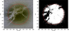Fig. 1 Left: trailing hemisphere of Dione colour map built with images from IR, green, and UV filters of the Cassini/ISS cameras (Schenk et al. 2011). The red perimeter encircles the region where the IR/UV ratio is at least 1.3, corresponding to a latitudinal extension of ~± 65° at longitude 270W. Right: mask of the ROI used to sort both CIRS FP1 observations and the GTM tiles.

2 Region of interest: Properties and observations

The Voyager flybys revealed large geologic scars that indicate a recent resurfacing (Stephan et al. 2010; Plescia 1983). The trailing hemisphere of Dione exhibits geologically younger regions consisting of a network of bright linear or curved lineaments, the wispy chasmata – which may have resulted from tectonic activity – embedded in densely cratered older plains (Stephan et al. 2010). The reddening and darkening of this hemisphere, thought to be linked to the interaction with cold plasma flow, is clearly visible in the IR-green-UV colour map provided by the Cassini/ISS (Imaging Science Subsystem) camera (Fig. 1, left; Schenk et al. 2011).

2.1 Chemical composition from VNIR observations

Newman et al. (2009) analysed some Cassini/VIMS (Visible an Infrared Mapping Subsystem) VNIR reflectance spectra of this hemisphere acquired early in the mission (2004–2005). They found a lower level of crystallinity and shallower water-ice bands in the dark and densely cratered plains compared to the wispy chasmata. This may originate either from the contamination by non-water-ice material or from the existence of smaller grains of pure water ice, the size of which was evaluated at 1–8 μm. Thanks to a spectral classification of VIMS data, Stephan et al. (2010) later found that bombardment by magnetospheric particles is consistent with the concentration of dark material and enhanced CO₂ absorption on this hemisphere, independent of the geology. They identified spectral units #5 and #6 in those plains with spectral slopes of the continuum between 0.5 and 0.35 μm and 0.5 and 2.3 μm and with water-ice BD1 and BD2 at 1.5 and 2 μm, respectively (Table 1). These units exhibit the highest amount of non-ice material and the exclusive presence of the minor compound CO₂. The authors did not propose any estimate of grain size there. Scipioni et al. (2013) also performed a spectral classification on a still wider data set, but limited to the near-IR channels. They characterised these same dark terrains as two end members (spectral units #1 and #2), the BDs of which were found comparable to that produced by pure ice grains of 1–3 μm (which is similar to the Newman et al. (2009) results), or as 25-μm-sized grains intra-mixed with darkening material (AmC at 50–70% levels). The spectral slope VIS3, between 1.1 and 2.25 μm, appears the flattest for these regions (Table 1). Dalle Ore et al. (2021) examined the phase of water ice on this hemisphere and evaluated the amorphous ice fraction from some VIMS spectra. With an intimate mixture of 10–14-μm-sized water ice grains and 20-μm-sized AmC grains with 90–93% and 10–7% volume fractions, respectively, the amorphous water ice fraction was found to be 20% on average and would result from the bombardment by magnetospheric particles and be partially compensated by re-crystallisation during diurnal thermal cycle.

Filacchione et al. (2012) included the VIMS visible channel in their analysis for the leading hemisphere only and proposed an intra-mixture of 59-μm-sized grains made of an intramolecular mixture of crystalline water ice with 99.7% of the ice and 0.3% of the tholins (hereafter Th, to explain the spectral reddening from UV to VNIR), mixed with 11% of the same-sized grains of AmC. The NIR neutral or bluer slope is a function of grain size and amount of darkening contaminant for which AmC is usually used and intimately mixed. As noted by Poulet et al. (2002, 2003) in their study of Saturn’s rings, only a complex carbon compound such as tholins can reproduce the UV-to-NIR reddening. Poulet et al. (2003) reproduced spectra of the main rings with 10 μm-sized AmC grains intimately mixed with water-ice grains of various sizes and intramolecularly mixed with Th at 0.41–0.74% levels. Finally, the bolometric Bond albedo, A, derived by Pitman et al. (2010) with the VIMS-observed NIR geometric albedo and phase integral, is 0.37 ± 0.08, which is consistent with the estimate of A = 0.39 ± 0.13 derived independently from CIRS observations by Howett et al. (2014).

2.2 Topography

The Dione GTM built by Gaskell et al. (2008) was used here to characterise its topography both globally and within the CIRS FP1 footprints. It is organised as a set of 6q²+2 vectors in an implicitly connected quadrilateral form. This corresponds to a ground sample distance (GSD) of $\sim \pi R_D/2\sqrt{3}\mathrm{q}\sim 8\mathrm{k}\mathrm{m}$ for q=64 given Dione’s radius, R_D (Gaskell et al. 2008). Roughness is usually described by a typical slope for a given scale and assessed differently among authors (Shepard & Campbell 1998; Labarre et al. 2017). Here, the slope, θ, relative to the local ellipsoid was estimated for each tile of the tessellated surface for q = 64 and the best available resolution q = 512, i.e. a GSD of ~1 km. Resulting from the tessellation process and the selection of images, the global distribution of slopes is found to be best described by a log-normal probability density function of p_Ln(θ, q) rather than a Gaussian or even a Rayleigh one. This kind of distribution is known to result from a random process where various effects combine multiplicatively, in particular for 2D or 3D processes, and to maximise the entropy (Limpert et al. 2001; Grönholm and Annila 2007). Its global mean ${\overline{\theta }}_{Ln}$ and standard deviation σ_Ln increase with decreasing GSD, typically from ${\overline{\theta }}_{\mathrm{L}\mathrm{n}}$ = 3.7° and σ_Ln = 4.7° for q = 64 to ${\overline{\theta }}_{Ln}$ = 5.8° and σ_Ln = 7.1° for q=512. The mean values are very close to the RMS slope ${\theta }_{\text{RMS}}=\overline{{\theta }^2\cos \theta },{4.1}^{\circ }$ and 6.1°, respectively (Davidsson et al. 2015). Maximum slopes θ_max are 24.2° and 34.8°, respectively. Roughness can be similarly estimated within each FP1 footprint, j, which is the projection of the field of view on the ellipsoid, (hereafter the FOV). The distributions at this scale are also clearly log-normal, so ${\overline{\theta }}_{Ln}$(j) and σ_Ln(j) can also be derived at a given GSD.

2.3 CIRS observations in the region of interest

The CIRS database has been browsed to extract FP1 observations of the trailing hemisphere and retain those that cover a good proportion of the region of interest (ROI) with footprints containing no more than a few thousand tiles overall, i.e. a few tens of degrees with a resolution of 0.8 °/tile (q=64; Table 2), thereby limiting the calculation time in the various steps of this study. These observations cover a wide range of local times at various viewing and illumination geometries over a ten-year period during which the solar distance increases by nearly 1 au. Observations # 2, 3, 8, 10, and 11 were made at approximately dusk or dawn, while # 1, 4, 5, 6, 7, and 9 happened during daytime. Incidence i, emission e and phase α angles relative to the reference ellipsoid at the centre of the FOVs are plotted in Figure 4. Typical average incidence and emission angles relative to tiles normals within footprints and their standard deviations are also plotted.

In order to select FP1 footprints that are filled by at least 90% with this red and dark material, the IR-green-UV colour map produced by Schenk et al. (2011)¹ was used; from this, an IR/UV image was calculated and then set as the threshold at the ratio 1.3, which corresponds to the maximum of this ratio for the leading hemisphere (Schenk et al. 2011). This segmentation clearly isolates a quasi-circular ‘bulls-eye’ shape resulting from the interaction of plasma (Hendrix et al. 2012; Cassidy et al. 2013), with a diameter at the equator at ~± 65° longitude around 270 W (Fig. 1 right). In this mask, the brightest geological structures can be distinguished in black. A 25-pixel median filter was finally applied to the mask to reduce small isolated areas and a salt-and-pepper effect resulting from the threshold.

3 Modelling regolith properties

The temperature, T_S, of any surface element is determined at any time by the energy balance at the surface (z=0) between the absorbed solar spectrum in the VNIR domain, the thermal emission in the IR, and the heat flux from deeper layers: $${\mu }_{0,L}{\int }_{VIS}(1-r_h(\lambda ))\frac{C(\lambda )}{D^2}d\lambda ={\int }_{IR}{\epsilon }_h(\lambda )B(T_S,\lambda )d\lambda -k_E\frac{\mathrm{\partial }T}{\mathrm{\partial }z}{|}_{z=0},$$(1)

where μ_0,L = sin(i_L), i_L is the local solar incidence angle, C(λ) the air-mass zero solar spectrum ASTM-E490 measured at Earth, D the heliocentric distance in astronomical units, B(T, λ) the Planck function, and r_h(λ) and ε_h(λ) the hemispherical reflectance and emissivity, respectively (Eqs. (A.4) and (A.1)). The observed thermal emission within any FOV may indeed differ from a blackbody curve, as many tiles with various thermal histories contribute to it. The thermal conduction, k_E, at depth, z, is expected to essentially depend on the structure of the regolith, i.e. its porosity, the grain size, the ice phase, the contact quality, and the temperature (Ferrari & Lucas 2016). Making the most of the information available a priori concerning ε_h(λ) and r_h(λ) can improve our understanding of this boundary condition and provide an initial assessment of the quality of thermal conduction. Reflectance spectroscopy yields constraints on size in the very upper layers, which absorb solar light (i.e. the bolometric Bond albedo A, Eq. (A.5)). The Hapke formalism used in the model allows for a consistent description of the absorption and emission of the regolith layers (Hapke 2012; Ferrari 2024). A summary can be found in Appendix A.

3.1 Reflectance and bolometric Bond albedo A

The possibility of complying with VNIR spectral constraints exclusively with an intramolecular mixture of water ice, amorphous (AmI) or crystalline (Ih), with Th and/or AmC is explored here, following Filacchione et al. (2012) and Poulet et al. (2003). Spectral slopes and BDs were estimated from the modelled hemispherical reflectance, r_h(λ, a), at reference wavelengths while BDs follow the definition BD = 1 – RB/RC, where RB = r_h(λ_ref) and RC is linearly interpolated from the continuum at λ_ref. The correction for diffraction as proposed by Joseph et al. (1976) is chosen. The reader is referred to Ferrari (2024) for information on the optical constants of the various materials and a commentary on the complexity of developing them consistently over a wide wavelength range from the UV to far-IR. Those used here are listed in Appendix A. Intramolecular mixing with the three compounds is calculated with the Maxwell–Garnett formulation and mixing fraction, f, within the a priori range [0.05–3%] (Wu et al. 2018).

3.2 Infrared emissivity

In Ferrari (2024), the Hapke isotropic multiple scattering approximation (IMSA) model (Hapke 2012) was implemented to study the sensitivity of the hemispherical emissivity ${\epsilon }_h^{\ast }$(w_n, a, ice, ξ) to icy regolith properties and parameters such as types of diffraction correction or of mixing with contaminants with water ice or such as the size a of regolith grains, and the regolith average asymmetry factor, ξ, in case of anisotropic and multiple scattering. The influence of contaminants on the IR spectra only matters above a certain percentage level and most significantly when the mixture takes place on a molecular scale (Ferrari 2024).

Were the regolith considered a blackbody surface, the emitted spectrum measured in the FOV would resume to I(w_n) = B(T, w_n) as a function of wave number, w_n = λ⁻¹, and surface temperature, T. For a smooth regolith, as assumed in the original model M_o (Ferrari 2024), it is written $$I\left(w_n\right)={\epsilon }_h^{\ast }(w_n,a_o,{\xi }_o,ice)\times B(T_o,w_n),$$(2)

following the nomenclature of model factors established in Table 3.

The first inferences of model factors with this model yielded an asymmetry factor of ξ_o correlated with the solar incidence angle, whereas it should not be as it is an intrinsic property of the regolith (Fig. 4c, Sect. 4.2). The underlying dependence of thermal emission at this particular angle led us to consider adding a shadowing function to complete the original model. One may indeed expect roughness at a given spatial scale to affect the thermal emission received from differently oriented and heated slopes. The thermal inertia of Dione being very low, thermal equilibrium may be reached fairly quickly, so the shadowing effect on thermal emission is similar to that influencing reflectance. The scale at which this roughness is active remains unknown, and it may be on the grain scale (Shepard et al. 2001; Labarre et al. 2017). The effect of roughness on thermal emission has been studied for decades on rocky planetary bodies (Smith 1967; Spencer 1990; Lagerros 1996; Davidsson et al. 2015). In the literature, several shadowing functions have been proposed to mimic this effect either in reflectance or in thermal emission (Shepard & Campbell 1998; Davidsson et al. 2009, 2015). Most of the analytical formulations, which are most practical for data inversion, assume a Gaussian distribution of slopes, which appears not to be relevant here (as far as GTMs do correctly reflect real slopes). The Hapke shadowing function, S(i, e, α, ${\overline{\theta }}_H$), is expected to model the effect of shadows in the measured radiance of a surface seen at illumination; emission; and phase angles i, e, and α relative to the reference ellipsoid, depending on the mean slope, ${\overline{\theta }}_H$, averaged over all spatial scales. This model assumes the topography to be Gaussian and slopes to be small, in which case their distribution should tend towards a Rayleigh one (Shiltz & Backman 2023). Despite these limits, it remains a benchmark model for estimating roughness. For this new model, hereafter noted M_H (H for Hapke), the IR emission may be written as $$I\left(w_n\right)={\epsilon }_h^{\ast }(w_n,a_H,{\xi }_H,ice)\times S(i,e,\alpha ,{\overline{\theta }}_H)\times B(T_H,w_n),$$(3)

where ${\overline{\theta }}_H$ is the mean roughness within the FOV. The case of an isotropic scattering was also tested with a model hereafter noted M_iH (iH for isotropic Hapke), adjusting the spectrum by exchanging I(w_n) in Eq. (3) with ξ_H = 0 (Table 3).

Finally, with the help of the NAIF Spice kernel library (Acton et al. 2018; Annex et al. 2020), it was also possible to derive, from the GTM, an estimate of the shadowing function for scale q (noted S_q(i, e, α)) as defined in Hapke (2012) in Eqs. (12.22) and (12.23), based on the probability that a tile is both illuminated and visible, given i, e, and α from ephemeris to date. It can be estimated for each FOV pointing, j, and tiles within. Thus, this M_q model assumes $$I\left(w_n\right)={\epsilon }_h^{\ast }(w_n,a_q,{\xi }_q,ice)\times S_q(i,e,\alpha )\times B(T_q,w_n).$$(4)

The assumptions and nomenclature of factors of models M_o, M_H, M_iH, and M_q are listed in Table 3.

3.3 Metric for comparing models and deriving their factors

Given the j^th spectrum, I_obs,j(w_n), acquired among N_po pointings found in the ROI during an observation (Table 2), the temperature, T_j, for which B(T_j, w_n) best fits I_obs,j(w_n)/ε_a(a, ξ, $\overline{\theta }$, w_n) is determined, where ε_a(w_n) is either ${\epsilon }_h^{\ast }(w_n)$ or ${\epsilon }_h^{\ast }(w_n)\times S(i,e,\alpha ,\overline{\theta })$. The reduced residual is then $${\chi }_R^2(j,a,\xi ,\overline{\theta })=\frac{1}{N_{w_n}}\sum _{w_n}{(\frac{I_{obs,j}\left(w_n\right)}{{\epsilon }_a\left(w_n\right)}-B(T_j,w_n))}^2\frac{1}{NESR{\left(w_n\right)}^2}$$(5)

for each set of factors (a, ξ, $\overline{\theta }$). NESR is the noise equivalent spectral radiance (Flasar et al. 2004), and N_wn is the number of points in the spectrum. The best solution for each spectrum (a_j, ξ_j, ${\overline{\theta }}_j$, T_j) was derived by minimising ${\chi }_R^2$(j, a, ξ, $\overline{\theta }$). A global solution for each observation, i.e. $(\overline{a},\overline{\xi },\overline{\overline{\theta }})$, was inferred by minimizing as follows: $${\overline{\chi }}^2(a,\xi ,\overline{\theta })=\frac{1}{N_{po}}\sum _j{\chi }_R^2(j,a,\xi ,\overline{\theta }).$$(6)

The corresponding spectral residuals, average R²(w_n), or global ${\overline{R}}^2$(w_n), are written as $$R^2\left(w_n\right)=\frac{1}{N_{po}}\sum _j{(\frac{I_{obs,j}\left(w_n\right)}{{\epsilon }_a(a_j,{\xi }_j,{\overline{\theta }}_j,w_n)}-B(T_j,w_n))}^2\frac{1}{NESR{\left(w_n\right)}^2},$$(7) $$R^2\left(w_n\right)=\frac{1}{N_{po}}\sum _j{(\frac{I_{obs,j}\left(w_n\right)}{{\epsilon }_a(\overline{a},\overline{\xi },\overline{\overline{\theta }},w_n)}-B(T_j,w_n))}^2\frac{1}{NESR{\left(w_n\right)}^2}.$$(8)

These spectral residuals can still be averaged over wave numbers as well and provide mean R² and mean global ${\overline{R}}^2$ residuals, respectively. Those quantities are used as a metric to compare the ability of various models to predict observed spectra.

4 Results

4.1 Surface grain size and water-ice contamination

Initially, an intra-molecular mixing of water ice with either Th or AmC alone was considered, before proposing a mixture with the three components. In case of the Th contaminant alone, BD 1, and BD 2 are weakly dependent on f, mainly modulated by grain size; the BD1 value is easily reproduced with grains in the 0.2–3 μm range, and that of BD 2 is either 0.2–0.3 or 4–7 μm. These marginally exclude each other and are thus compatible with the range put forward by Newman et al. (2009) for pure water-ice grains. The Bond albedo A is instead highly sensitive to f, which has to be >3% for the micrometer-sized grains to fit Pitman et al. (2010) values. The VIS1 slope strongly depends on f and remains too high on average for sizes in the 0.1–100 μm range, but for f < 0.1%. The VIS2 slope obeys constraints for f = 0.1% and grains larger than 0.5 μm. The VIS3 slope does not meet requirements, except for centimetre-sized grains. With an AmC contaminant only, an intramolecular mixture with f < 0.1% can reproduce BD1 with 2–6 μm-sized grains and BD2 with grains of <0.2 μm or 7–9 μm, which marginally exclude each other. Albedo A is in the right range with micrometre-sized grains if 0.1% < f < 0.5%. With such a mixing level, the slope of VIS1 can hardly be reproduced with sizes of 0.7 to a few μm, while VIS2 is only within the observed range for sub-micrometre grains. VIS3 can be reproduced with a > 1 μm. For f < 0.5%, an intra-molecular mixture with AmC can satisfy A, BD1, BD2, and VIS3 constraints for micrometer-sized grains, but this is only marginally the case for VIS1 and VIS2.

Mixing finally both contaminants at similar levels within micrometre-sized grains can easily darken the regolith. Even a small fraction – 0.05%<f<0.1% – of AmC impacts the A albedo, slopes, and BDs significantly for a given size (Fig. 2d). It is easy to reach the VIS1 slope with Th (Fig. 2b). Intramolecular mixing with AmC grains at a low fraction (typically 0.1%) can help recover BD 1 and BD 2 (Fig. 2a), VIS 3 or A ones, whereas a small fraction of Th (typically 0.1%) provide the expected VIS1 constraint (Fig. 2b). Slope VIS3 and BD1 constrain the sizes to 2–5 μm with an f of 0.05–0.1% (Fig. 2c), which is compatible with Bond albedo A (Fig. 2d) and VIS1 (Fig. 2b) constraints. BD 2 is marginally compatible with this; the observed slope of VIS2 remains too large compared to the modelled one. The ice phase has some impact on BDs and slopes, but only a weak impact on A. Bearing in mind that these comparisons are made with optical constants at a given temperature (see Appendix A), the order of magnitude on f, sizes (μm), and the nature of contaminants can be considered plausible in an intra-molecular mixing scenario. The sizes are comparable to those obtained through other studies and with the Bond albedo measured by different means both in the near-IR and thermal IR. An equal amount of Th and AmC contamination at intramolecular level is plausible.

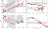Fig. 2 Spectral indicators: VNIR constraints and modelled ones. Constraints from VNIR observations as given in Table 1 correspond to the shaded zones. Modelled indicators are plotted as a function of grain size a, which is composed of an intra-molecular mixture of water ice, either crystalline hexagonal (Ih, solid line) or amorphous (AmI, dashed line), with AmC and Th, with a fraction of f = 0.05% (red) or 0.1% (black). The size is regularly indicated (in μm) along the curves: (a) BD2 versus BD1; (b) VIS2 versus VIS1; (c) VIS3 versus BD1; (d) A versus a. Bolometric Bond albedo constraints inferred from IR observations by Howett et al. (2014) are also plotted (dotted line).

4.2 Properties of a smooth regolith (M_o model)

The observation with the best spectral resolution (#1, 2.85 cm⁻¹, Table 2) was analysed first. It consists of a north-south scan at good spatial resolution between latitudes of ±15° around the equator. With the smooth regolith model, M_o, and assuming a mixture of Ih water ice with f=0.1% Th and AmC, temperatures of T_j, sizes of a_j, and asymmetries of ξ_j were retrieved according to Eq. (5), together with the global average grain size, ${\overline{a}}_o$, and asymmetry factor, ${\overline{\xi }}_o$ (Eq. (6)). The best size is ${\overline{a}}_o$ = ${50}_{-20}^{+49950}$μm at 1σ (or ${\overline{a}}_o$ > 30 μm) and ${\overline{\xi }}_o$ = ${0.9}_{-0.9}^{+0}$ (on the boundary of the allowed range).

An observed mean hemispherical emissivity of ${\overline{\epsilon }}_{obs}$(w_n) with a standard deviation of σ_obs(w_n) can be estimated from the average, $${\overline{\epsilon }}_{obs}(w_n)=\frac{1}{Npo}\sum _j\frac{I_{obs,j}\left(w_n\right)}{B(T_j,w_n)},$$(9)

and compared with the hemispherical emissivity, ${\epsilon }_h^{\ast }({\overline{a}}_o,{\overline{\xi }}_o)$, or the mean hemispherical emissivity, ${\overline{\epsilon }}_{mod}$(w_n), of the best models, ${\epsilon }_h^{\ast }(a_j,{\xi }_j,w_n)$, obtained for each spectrum (Eq. (5), Fig. 3 top) with $${\overline{\epsilon }}_{mod}(w_n)=\frac{1}{Npo}\sum _j{\epsilon }_h^{\ast }(a_j,{\xi }_j,w_n).$$(10)

The presence of the roll-off at w_n < 50 cm⁻¹ favours the predominance of grains larger than 100 μm. The slight rise below 35 cm⁻¹ is indicative of sizes of only a few tens of micrometres (Fig. 3, Ferrari 2024). The best model spectra still present a spectral feature due to peak water-ice absorption near 222 cm⁻¹ due to lattice vibration, which is not present in the observed ones (Fig. 3 top).

The global spectral residual, ${\overline{R}}_o^2$(w_n), is found to be much smaller than the ‘blackbody’ model residual $R_B^2$(w_n) in the roll-off region (w_n < 50 cm⁻¹; Fig. 3, bottom). Part of the error (20%) is due to fluctuation in observed spectra of about 90 cm⁻¹ in observation #1, the source of which seems unrelated to identified noise. The M_o model provides a better prediction with a mean global residual (averaged over w_n) ${\overline{R}}_o^2$ = 2.6 ~ $R_o^2$ against ${\overline{R}}_B^2$ = 5.0. Some residuals appear above noise at low w_n <30 cm⁻¹ or in between 105 and 200 cm⁻¹, a region where superficial grains remain highly absorbent (Fig. 3 bottom). However, caution should be exercised when interpreting these remaining residuals, as variations in optical constants of ice and contaminants and/or other effects, such as variations in geometry from one spectrum to another, were not taken into account at this stage. Decreasing f does not change the result. With amorphous ice AmI, the mean global and average residuals, ${\overline{R}}_o^2$ and $R_o^2$, remain similar (3.14 and 2.9), with a solution ${\overline{a}}_o$ > 0.3 mm at 1σ and ${\overline{\xi }}_o$ = ${0.1}_{-0.6}^{+0.7}$, within the permitted range (Table 4). The fit with the original model M_o and 75% AmC contaminants intimately mixed in water ice as proposed by Carvano et al. (2007) gives worse residuals (${\overline{R}}_o^2$ = 4.3, $R_o^2$ = 4.1), in particular in the roll-off region.

Second, this model was adjusted to all observed spectra according to Eq. (5) (Table 2). The viewing and illumination geometry relative to the reference ellipsoid is plotted in Figures 4 a and 4b. Constraints on the asymmetry factor, ξ_o, were only obtained when the regolith was lit (i < 90°) and, more precisely, when i < 45–60°, for observations # 1, 4, 5, 6, and 7 (Figs. 4a, c, and Fig. B.1 with error bars, Table 2). The thresholds for this factor beyond which the solutions are not physical are set at ±0.9. Its correlation coefficient with i is strong for # 1, 6, and 7, and weaker for # 4 and 5. The correlation looks very similar between # 6 and 7, which share close illumination and viewing geometries. Both consist of north-south scans at almost constant and nearly noon local time (Table 2). Except for i < 35°, temperatures, T_o, for both observations smoothly vary with i and roughly follow a cos(i)^1/4 trend, as expected for a flat surface of low thermal inertia at a given local time (Fig. 4d). This is also the case for the morning observations # 4, 5, and 9. Despite the morning local time, observation #1 exhibits higher T_o when i is similar to noon observations, but it happened when Saturn was closer to the Sun (Table 2). The average difference among pointings of temperatures inferred with model M_o and the blackbody model is $\overline{T_o-T_B}=1.12$ K. The global solutions (${\overline{a}}_o,{\overline{\xi }}_o$) minimising ${\overline{\chi }}^2$ (Eq. (6)) for each observation are given in Table 4 in the case of an AmI mixture with 0.1% AmC and Th. Results are insensitive to the mixing ratio at the levels considered here, as expected (Ferrari 2024). The best residuals, ${\overline{\chi }}_o^2$, obtained with model M_o are two-to-four-times smaller than the residuals obtained assuming blackbody behaviour, ${\overline{\chi }}_B^2$ (Table 4), and they are most often two times smaller with amorphous AmI than with Ih water ice, except for #1 and 9, for which they are similar. This aspect may warrant further study. The grain sizes, ${\overline{a}}_o$, found are relatively well determined, within the 1–3 mm range, which is consistent with the range provided by observation #1.

Fig. 3 Observed and best mean hemispherical emissivities. Top: hemispherical emissivities as a function of wave number for observation #1: mean observed (Eq. (9), red), mean of best models (Eq. (10)) and their standard deviations (dotted lines), and best model across all spectra (black) obtained with model Mo. Bottom: spectral residuals R2(wn) (Eq. (7)) and ${\overline{R}}^2$(wn) (Eq. (8)) obtained with blackbody model ($R_B^2$) or smooth model, Mo($R_o^2$ or ${\overline{R}}_o^2$). Mean and mean-global residuals are plotted as dashed lines. The intra-molecular mixture is AmC and Th at 0.1%, each within a matrix of Ih crystalline ice. The lattice vibration at 222 cm−1 and instrumental fluctuation about 90 cm−1 are indicated (vertical dotted lines).

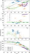Fig. 4 Results with smooth surface model, Mo. (a) Emission, e, versus incidence, i, angles of all pointings for daytime observations as numbered in Table 2. These angles are relative to the normal of the reference ellipsoid at the centre of the FOV. Mean (x symbol) and standard deviation (error bars) of local incidence and emission angles on tiles within footprints at the start, middle, and end of observations are also plotted. (b) Phase angle, α, of pointings versus i. (c) Asymmetry factor, ξo, versus i inferred for each pointing, j. (d) Temperatures of To versus i inferred for each pointing j. Temperature dependences with i such as Tm cos(i)1/4 are plotted for Tm = 98, 106, and 112 K. Error bars on To are plotted and are very small. The intra-molecular mixture of amorphous water ice with 0.1% Th and AmC is assumed.

4.3 Roughness

Considering a smooth surface provides good constraints on grain size and reveals, in daytime observations, an non-physical anti-correlation of the intrinsic regolith property, ξ, with i. An analysis of the sensitivity of the M_o model to its factors shows that it is essentially sensitive to grain size in the roll-off region, while it becomes relatively more sensitive to ξ in the water ice absorbent region about 150–300 cm⁻¹ (Ferrari 2024). The asymmetry factor indeed figures multiple or anisotropic scatterings, which modulate the average scattering albedo and therefore the emissivity. For daytime observations, this anti-correlation suggests an un-modelled effect – which lowers emissivity as the incidence angle increases – and that a shadowing function may simulate in most favourable situations when the observer’s direction is sufficiently far from the Sun’s direction to see the shadows. A known topography can be integrated into a thermal model to estimate its effect on temperature or emissivity in the FP1 FOV (Ferrari et al. 2021). However, this remains a topography on a kilometre scale at best, whereas smaller scales can influence radiative balance and heat flow. Before moving on, for these more time-consuming simulations, it is advisable to explore the ability of simpler models, albeit assuming low thermal inertia and rapid radiative equilibrium, to improve prediction of spectra. The next step is to examine both the local properties in each FOV – i.e. (a_j, ξ_j, ${\overline{\theta }}_{H,j}$, T_j) – when the Hapke shadowing function is included, and the global best solutions $({\overline{a}}_H,{\overline{\xi }}_H,{\overline{\overline{\theta }}}_H)$ for daytime observations.

4.3.1 Properties of a rough regolith (M_iH and M_H models)

The fit with the rough model M_iH, including the Hapke shadowing function, S(i, e, α, ${\overline{\theta }}_{iH}$), and isotropic scattering, ξ_H=0, provides better global fits (${\overline{\chi }}_{iH}^2$) to all observations (Table 4). The grain size, ${\overline{a}}_{iH}$, remains relatively well constrained at about 1–2 mm. Observation #1 differs in geometry, e ≳ i, and small phase angle, α (Fig. 4a). Even though some ${\overline{\theta }}_{iH}$ values remain consistent with observations #6 and 7 at a similar i, several are found to be different at i ~ e ~ 45°. This could be evidence of geographical changes that warrant further detailed investigation (Fig. 5 or Fig. B.1 with error bars). The same roughness of ~17° is measured for observations #4, 5, and 9; it was obtained at very diverse epochs, at higher i, and at lower e for various phase angles, a configuration that is most favourable for constraining shadowing and roughness. A larger one of ~30° is inferred for observations #6 and 7 (Table 4). The roughnesses, ${\overline{\theta }}_{iH}$, are very close and consistent as a function of i for both observations scheduled one hour apart. The error bars are larger when e is close to i and the phase angle small, as shadows disappear and emissivity becomes less sensitive to them. As i increases, errors decrease, and the estimated roughness is almost constant and coherent between both observations. However, the error bars on the values obtained when i ≤ 25° are very large and make them consistent with the other observations. The significance of roughness decreasing with illumination is thus uncertain. The average of differences is $\overline{T_{iH}-T_B}$ ~ 3.3 K, which is significantly higher than for the smooth model (Fig. 5, bottom). A rough model thus significantly improves the prediction of spectra under the assumption of low thermal inertia.

Adding a non-zero asymmetry factor, ξ_H, (M_H model) only marginally improves the overall fit (Table 4). The roughnesses, ${\overline{\theta }}_H$, decrease by about a degree compared to the ${\overline{\theta }}_{iH}$, grain sizes may occasionally increase by one millimetre, which is within error bars. Adding roughness, on the other hand, refocuses the global ${\overline{\xi }}_H$ values around zero, whereas the ${\overline{\xi }}_o$ were stuck at the lower limit of −0.9 (Table 4). The results for the M_H model confirm that the assumption of a zero asymmetry factor is a reasonable one, its cost being low. Temperatures, T_H, are almost similar, and the average difference is $\overline{T_H-T_B}$ ~ 3, 5 K. The results with crystalline water ice are systematically worse by a few ${\overline{\chi }}^2$ units, while the roughness estimates change little, the sizes are often smaller (about a few hundred micrometres sometimes), and the ${\overline{\xi }}_H$ values are larger (and also compatible with ξ_H = 0).

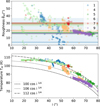Fig. 5 Results with rough model with isotropic scattering MiH. Top: roughness, ${\overline{\theta }}_{iH}$, versus solar incidence, i, inferred for each pointing, j, of daytime observations. Bottom: temperatures, TiH. The shaded zone and horizontal coloured lines correspond to best global fits per observation: ${\overline{\overline{\theta }}}_{iH}\pm \mathrm{\Delta }{\overline{\overline{\theta }}}_{iH}$ (Table 4). The intra-molecular mixture of amorphous water ice with 0.1% Th and AmC is assumed.

4.3.2 Properties of rough regolith on an 8 km scale (M_q model)

The fit using the shadowing function S_q(i, e, α) as derived from the GTM (Eq. (4)) does not provide better results than any other rough model (Table 4). The anti-correlation of ξ_q with i remains, with some values still at the limit of the fitting range mainly for i ≥ 50°, but it appears more consistent between observations compared to the smooth M_o model (Fig. 6b; Fig. B.1 with error bars; Fig. 4c). The derived sizes, ${\overline{a}}_q$, are consistent with the other models, with somewhat smaller error bars (Table 4). The average difference is $\overline{T_q-T_B}$ ~ 2.2K (Fig. 6c). With a different way of evaluating the shadowing function (directly from the GTM and the astrometry, without any assumption on the distribution of slopes), this model is better than the smooth one and remains close to the rough ones, but the anti-correlation persists. The actual origin of this effect does not appear to be on the scale of the 8 km topography. The average slopes, ${\overline{\theta }}_{Ln}$, estimated in each FOV from the 8-km-scale GTM are shown for all daytime observations in Figure 6a. The highest dispersion among them is observed in #1. They are much smaller than the ones derived from the other rough models (Fig. 9 for a direct comparison).

Finally, the superposition (multiplicatively) of both shadowing effects S_q(i, e, α) and S(i, e, α, ${\overline{\theta }}_H$), assuming both overlap at different scales, gives results very close to the M_H model, occasionally slightly better but not significantly. The asymmetry factors ξ_q+H can be seen with error bars in Figure B.1. Here again, the adjustments are less effective with crystalline ice.

4.4 Nighttime, dawn, and dusk observations

Observations at dusk (#2 and 3, Table 2, Fig. 7) provide only weak constraints on grain size, i.e. ${\overline{a}}_o$ ≥ 3–4 mm in the case of a smooth surface, and essentially none on ξ_o. When assuming an isotropic scattering and a rough terrain (M_iH model), the minimum size stays of the order of a millimetre, and roughness is found to be zero, which is compatible with the disappearance of shadows and contrasts in radiance. No constraints can be obtained for spectra measured at dawn (#8, 10, or 11). The fit with a rough surface and isotropic emission also yields null roughness. A temperature can certainly be derived at these local times assuming known regolith properties or at least a blackbody behaviour. In fact, the average residual, $R_B^2$, for a blackbody model is of the same order of magnitude as that of models M_o and M_iH for these observations.

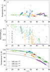Fig. 6 Results with rough model, Mq, for daytime observations. (a) Roughness, ${\overline{\theta }}_{Ln}$(j), as determined a priori from the GTM versus i. (b) Asymmetry factor, ξq, versus i. (c) Temperatures, Tq, versus i. Error bars on Tq are plotted and are very small. The intra-molecular mixture of amorphous water ice with 0.1% Th and 0.1% AmC is assumed.

4.5 Surface temperatures

Above the roll-off region (w_n ≥ 50 cm⁻¹), where the maximum thermal emission of an icy Saturnian regolith is expected to radiate, the emissivity is close to unity (Fig. 3). However, during daytime, if roughness also modulates the emitted spectra, the estimated surface temperatures may be significantly different from the blackbody estimates, T_B. These temperatures, derived from all spectra, and their deviation to the blackbody case, are displayed in Figure 7. The estimates from the M_H model are plotted for daytime observations, while the M_o model (smooth surface) is chosen for the others (#2,3,8,10, and 11). For the latter ones, the deviation, ΔT, is compatible with zero as expected, but it can be as high as 8.5 K in daytime observation # 9, for example, or of the order of 6–7 K around noon. Releasing the blackbody assumption therefore leads, as expected, to some systematic shift of temperatures to higher values and may somewhat alter the previously derived estimate of thermal inertia (Howett et al. 2010, 2014). The apparent diurnal thermal cycle displayed in Figure 7 has to be carefully analysed as it was built here with temperatures estimated at very different epochs and not corrected from solar distances (Table 2).

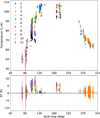Fig. 7 Surface temperatures versus local time. Top: temperatures, TH, for each pointing of observations listed in Table 2, inferred with the model MH for daytime ones or with Mo for the ones left over (Table 4). The blackbody temperatures, TB, estimated for the same spectra are plotted in black (+). Error bars on these estimates are about 1 or 2 K for dawn and dusk observations, and they decrease to 0.3 K at noon. Bottom: deviation ΔT = TH − TB for each pointing and their error bars. Local time is 0° at midnight and 180° at noon.

5 Discussion

5.1 Water-ice contamination

Observational constraints on spectral slopes, BDs, and the bolometric Bond albedo of the trailing hemisphere of Dione can be reasonably well reproduced by the reflectance of micrometresized grains made of water ice–either crystalline or amorphous–mixed at the intra-molecular level with tholins and AmC contaminants. This happens, interestingly, at comparable and low fraction levels of 0.05–0.1% at most. The Th fraction happens to be smaller than the 0.3% found on the leading hemisphere by Filacchione et al. (2012), the authors of which instead mixed those grains intimately with AmC grains. This mixing at the intramolecular scale may indicate a chemical alteration due to radiolysis. Non-water-ice materials detected on Dione include carbon dioxide (a few percent in terms of weight), hydrocarbons, and possibly cyanide compounds, while the presence of ammonia is still debated (Scipioni et al. 2013; Clark et al. 2008). The detected CO₂ may arise from the reaction of OH radicals with CO after the dissociation of H₂O molecules (Teolis and Waite 2016). Radiolysis of carbon-containing compounds, typically hydrocarbons or methane ice, by a variety of ions can yield CO₂ and complex organic material (Cassidy et al. 2010). The irradiation of water ice mixed with CO₂ by 10 keV electrons produces CO and H₂CO₃, with an upper limit of H₂CO, CH₃OH, and CH₄ at less than 0.5% of the remaining CO₂ (Hand et al. 2007). Less than one percent of CO₂ may lead to tenth of a percentage point of darkening carbon compounds and reddening hydrocarbons. The presence of nitrogen compounds may also yield many other products (Delitsky & Lane 2002; Sittler et al. 2006). This kind of contamination is compatible with a very superficial layer of micrometre-sized grains, as already derived from other studies but with other types of mixing. However, as already expressed by Hudson and Moore (2001), the chemistry of a multi-component icy regolith is complex to understand, and the mixing ratio of various components is still difficult to predict, even more so under the effects of sputtering and impact gardening. The proposed substitute of what is undoubtedly a very complex composition might merit a more detailed comparison with VIMS spectra.

5.2 Grain size

The introduction of a hemispherical emissivity depending on an effective grain size into a thermal emission model significantly improves the prediction of Dione’s observed spectra compared to a blackbody model. Its strong dependence on grain size below 50 cm⁻¹ allowed us to constrain it even with spectra of 15.5 cm⁻¹ resolution (Ferrari 2024). The daytime observations presented here, made at very different epochs, show with great consistency that the optimal grain size is approximately 1 or 2 mm. The lowest sized cut-off is 200 μm. The largest size may be a few centimetres (Table 4). Furthermore, this millimetre grain size is entirely compatible with the low thermal inertia observed on Dione, particularly if the water ice is in an amorphous phase and heat conduction happens concurrently through the pores (radiative) and the contacts between grains; this for a ‘normal’ porosity (Ferrari & Lucas 2016). While micrometre-sized grains control the bolometric albedo, the hemispherical emissivity averaged over the emission spectrum plays a role in the energy balance at the surface and depends on the regolith temperature (Eq. (2)). For grains larger than 200 μm, it varies little between 50 and 110 K, i.e. about 0.96–0.97 for grains of 5 cm, 0.95–0.97 for those of 1 mm, and 0.90–0.96 for those of 200 μm.

5.3 Absorption, extinction, and thermal skin depth

The absorption length Λ_c of solar flux can be approximated with the classical formulation for a continuous medium of Λ_c = λ/4πn_k. For the type of mixture and degree of contamination derived here, this length is about 100 μm in the visible domain and oscillates between depths of 10 and 100 μm in the middle IR (Fig. 8). If a regolith structure is assumed, the extinction mean free path, including both scattering and absorption, can be written as Λ_e(a) = 1/K_pE = 4a/3K_p(1 − p)Q_e, where E is the extinction coefficient, p the porosity of the regolith, and K_p the porosity coefficient (Eq. (A.8), Hapke 2012). The grain extinction efficiency, Q_e(a, λ), was corrected here from the diffraction peak. For a porosity, p =0.4, Λ_e(a) ~ a/Q_e(a, λ). For crystalline water ice grains larger than the wavelength, we find Q_e ~ 1 and Λ_e(a) ~ a.

Slightly contaminated micrometre-sized grains remain efficient at scattering solar light and significantly reduce the mean free path to their size range at VNIR wavelengths (Fig. 8). In the middle IR and around the maximum thermal emission of kronian surfaces, their extinction resumes to absorption, within lengths of 10–100 μm. These layers become transparent in the far-IR (λ ≥ 100 μm), so light emitted from greater depths and scattered by grains with sizes comparable to the wavelengths can be observed. Were the regolith isothermal down to this depth, the emissivity of those larger grains would possibly lower the brightness temperature in this roll-off region (Ferrari 2024). Were there a thermal gradient due to diurnal thermal cycle (the thermal skin depth is of the order of 5 mm; e.g. about a few Λ_e(a)), the brightness temperature would either be further amplified or reduced depending on the direction of the heat flux. The general trend does not change that much with the ice phase.

This is the image that can be constructed based on these thermal data and on the hypothesis of a regolith of spherical particles distributed into multiple layers. At this stage, it is difficult to say whether the superficial micrometre particles could constitute either the roughness of millimetre grains or millimetre-sized aggregates. Perhaps including the hemispherical emissivity based on the single scattering albedos of such objects in the models presented here could help. A detailed study of their photometric phase function with observations in the visible range could undoubtedly provide additional constraints on this pending question.

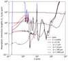Fig. 8 Absorption, Λc (solid line), and extinction, Λe(a), lengths versus wavelength, λ. Λe(a) is plotted for four grain sizes a of 1, 10, 100, and 1000 μm. The composition is Ih water ice, either pure (blue) or mixed on an intra-molecular scale with both AmC and Th contaminants at a fraction of f = 0.05% (red) or f = 1% (black). The porosity p = 0.4.

5.4 Surface roughness

Assuming zero thermal inertia and including roughness effects as a shadowing function described by the Hapke model improves the prediction of spectra (Table 4). The residual asymmetry factor, $\overline{\xi }$, is poorly constrained (M_H model), and assuming it to be zero remains appropriate at this stage (M_iH model). Our estimates of ${\overline{\theta }}_{iH}$ are much larger than the averages of the distribution of slopes within footprints (${\overline{\theta }}_{Ln}$) by at least one order of magnitude (Fig. 9, top). These values may differ because the assumptions made of small slopes and the Gaussian distribution of the Hapke shadowing function are not consistent with what was established from the GTM, or, they could be different because the roughnesses, ${\overline{\theta }}_{iH}$, impacting the thermal emission take place on a smaller scale. This is entirely possible as the study of natural surfaces shows that roughness increases towards smaller scales, by an order of magnitude between metre and centimetre scales (Shepard & Campbell 1998; Labarre et al. 2017). Surface roughness estimates for Dione are scarce in the literature. For Tethys and Rhea, the estimated values are 23 ± 5° and 16 ± 2°, respectively, and the photometric macroscopic roughness is set at 20° in the far-UV (see Verbiscer et al. (2018) for a review). The values derived here from thermal emission with a similar shadowing function are of the same order of magnitude (Fig. 9, top). By exploiting measurements at the nadir of the Diviner instrument aboard the LRO orbiter, Banfield et al. (2015) deduced an RMS slope of 20–35° from variations in lunar brightness temperature with the emission angle. The similarity between visible reflectance and IR emission estimates could indicate that roughness acts at wavelengths greater than 1 mm. It cannot be ruled out that the kilometre-scale roughness has some influence on the values of ${\overline{\theta }}_{iH}$. A correlation between average roughness, ${\overline{\theta }}_{Ln}$, in the footprints (Fig. 9, top) and latitude is high for observations #5, 6, 7, and 9, both visually and quantitatively. It is also true for ${\overline{\theta }}_{iH}$ in observations 5 and 9, and possible within error bars for #6 and 7 (error bars are large at positive latitudes). Secondly, ${\overline{\theta }}_{iH}$ are comparable to the steepest slopes observed at the 8 km scale (q=64; Fig. 9, bottom) and are therefore below the steepest slopes on a kilometre scale (q=512).

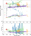Fig. 9 Latitudinal variations of roughnesses. Top: surface roughness, ${\overline{\theta }}_{Ln}$, either derived from GTM (cross) or estimated with the MiH model (${\overline{\theta }}_{iH}$, full circle). Dashed lines mark values derived for Tethys (23.5 ± 5°) and Rhea (16 ± 2°) trailing hemispheres. Bottom: ratio of ${\overline{\theta }}_H$ with the maximum slope of GTM within FOV footprints, i.e. θmax (GSD ~ 8 km).

6 Conclusions

Surface properties on the red and dark trailing hemisphere of Dione such as grain size and roughness were successfully extracted from CIRS observations by relaxing the assumption of blackbody behaviour. With a regolith model composed of multi-layered spherical particles and capable of consistently describing its hemispherical reflectance and emissivity, we found the following:

1. Superficial layers of micrometre-sized grains (2–5 μm) made of water ice contaminated at the molecular level with fractions as low as 0.1% of both amorphous carbon and tholins are shown to be compatible with band depths and slopes observed in reflectance;

2. In the far-IR, these layers are transparent to the radiation emitted by underlying millimetre-sized grains (1–5 mm), as inferred from the analysis of the hemispherical emissivity;

3. The daytime thermal emission is found to be sensitive to illumination and viewing geometry. Mimicking this effect with the Hapke shadowing function yields a better prediction of spectra and first estimates of roughnesses on this hemisphere, which range between 12° and 36° on average. These are larger than roughnesses measured on an 8-km scale in the shape model and may be typical of a smaller spatial scale;

4. Retrieved temperatures are higher when including effects of grain size and roughness. In this case, the asymmetry factor, ξ, is not constrained, and assuming that it is zero is correct. Nighttime observations can still be analysed assuming blackbody behaviour of the regolith;

5. Assuming amorphous water ice in emissivity models systematically provides better prediction.

This model can now be used to compare surface properties between the different hemispheres of Saturn’s icy moons and, when supplemented by IR thermal data, to enhance our understanding of the effects of space weathering at different locations in Saturn’s magnetosphere, all while respecting the constraints imposed by reflectance observations.

Acknowledgements

This work was supported by the Centre National d’Etudes Spatiales and the Programme National de Planétologie of CNRS – INSU through the ADSINTHE and PISTE projects.

References

Appendix A Model summary

What may be useful from Hapke’s theory used to develop the hybrid model in Ferrari (2024) is recalled here. The regolith is assumed to be populated with grains of uniform effective size a and composition (including phase of water ice, nature of contaminants, mixing type, fraction f). In case of isotropic scattering, the hemispherical emissivity of the regolith ε_h(w_n, a) is written at wavenumber w_n = λ⁻¹ as $${\epsilon }_h(w_n,a)\sim \frac{2\gamma (w_n,a)}{1+\gamma (w_n,a)}(1+\frac{r_0(w_n,a)}{6}),$$(A.1)

where $$r_0(w_n,a)=\frac{1-\gamma (w_n,a)}{1+\gamma (w_n,a)}$$(A.2)

and $$\gamma (w_n,a)=\sqrt{1-{\omega }_0(w_n,a)}$$(A.3)

as a function of the single scattering albedo of the grain ω₀(w_n, a), provided possibly by Mie’s theory. The hemispherical reflectance is approximated as follows: $$r_h(w_n,a)\sim 1-{\epsilon }_h(w_n,a)\sim r_0(w_n,a)(1-\frac{\gamma (w_n,a)}{3(1+\gamma (w_n,a))}).$$(A.4)

The bolometric Bond albedo is evaluated over the solar spectrum according to $$A(a)=\frac{{\int }_{\odot }(1-{\epsilon }_h(\lambda ,a))B_{\lambda }(T_{\odot },\lambda )d\lambda }{{\int }_{\odot }{B}_{\lambda }\left(T_{\odot }\right)d\lambda }.$$(A.5)

The delta-Eddington approximation is chosen to estimate the single scattering albedo ω_0,δE(w_n, a) after diffraction removal: $${\omega }_{0,\delta E}(w_n,a)=\frac{1-{\xi }_a^2}{1-{\xi }_a^2{\omega }_0}{\omega }_0,$$(A.6)

where ξ_a ≡ ξ(w_n, a) is the asymmetry factor of the scattering function of isolated grains and ω₀ ≡ ω_Mie(w_n, a) for a grain of size a as calculated with Mie’s theory.

In case of anisotropic and multiple scattering within the regolith and as far as hemispherically averaged quantities are concerned, the solution of radiative transfer equations can be approximated applying the similarity principle, which consists in replacing ω₀ with $${\omega }_0^{\ast }\left(w_n\right)=\frac{1-\xi }{1-\xi {\omega }_0\left(w_n\right)}{\omega }_{0,\delta E}\left(w_n\right),$$(A.7)

where ξ is the regolith average asymmetry factor (Hapke 2012).

The hemispherical emissivity ${\epsilon }_h^{\ast }(w_n)$ can be deduced with Eqs. A.1-A.3 and A.7. If ξ < 0, the regolith is more retro-diffusive and therefore less emissive, if ξ > 0, ${\epsilon }_h^{\ast }(w_n)$ will increase compared to the isotropic case (see Ferrari (2024) for more details).

The porosity coefficient K_p of a particulate medium, which scales the transmission through layers, is written as a function of porosity p as $$K_p=\frac{-ln(1-1.209(1-p{)}^{2/3})}{1.209(1-p{)}^{2/3}}.$$(A.8)

These calculations are performed here using the optical constants provided by various authors listed below. For crystalline water ice, data from Warren & Brandt (2008) and Mishima et al. (1983) at 90 K, Curtis et al. (2005) at 136 K, and Hudgins et al. (1993) at 120 K and have been merged. For amorphous water ice phase, the latest two have been replaced by Hudgins et al. (1993) data at 100 K. The optical constants for contaminants are those of Preibisch et al. (1993) for amorphous carbon (AmC) and of Khare et al. (1984) for tholins (Th).

Appendix B Inferred model factors with error bars

Error bars on inferred model factors are not displayed in the main core of the paper for clarity. The following figure shows asymmetry factors and their error bars as inferred with models M_o and M_q, displayed respectively in figures 4c and 6b, or ${\overline{\theta }}_{iH}$ roughness inferred with the rough surface model M_iH (Fig. 5) and finally the asymmetry factor ξ_q+H inferred by multiplicatively superimposing the two shadowing functions S(i, e, α, ${\overline{\theta }}_H$) × S_q(i, e, α), assuming they play at different spatial scales.

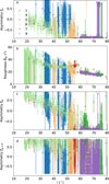Fig. B.1 Results from models presented in the main sections with error bars added. (a) Asymmetry factor ${\overline{\xi }}_o$ versus solar incidence angle, i. (b) Roughness ${\overline{\theta }}_{iH}$ versus i. (c) Asymmetry factor ξq versus i. (d) Asymmetry factor ξq+H versus i combining the shadowing functions of the Mq and MH models.

All Tables

All Figures

	Fig. 1 Left: trailing hemisphere of Dione colour map built with images from IR, green, and UV filters of the Cassini/ISS cameras (Schenk et al. 2011). The red perimeter encircles the region where the IR/UV ratio is at least 1.3, corresponding to a latitudinal extension of ~± 65° at longitude 270W. Right: mask of the ROI used to sort both CIRS FP1 observations and the GTM tiles.
In the text

Fig. 2 Spectral indicators: VNIR constraints and modelled ones. Constraints from VNIR observations as given in Table 1 correspond to the shaded zones. Modelled indicators are plotted as a function of grain size a, which is composed of an intra-molecular mixture of water ice, either crystalline hexagonal (Ih, solid line) or amorphous (AmI, dashed line), with AmC and Th, with a fraction of f = 0.05% (red) or 0.1% (black). The size is regularly indicated (in μm) along the curves: (a) BD2 versus BD1; (b) VIS2 versus VIS1; (c) VIS3 versus BD1; (d) A versus a. Bolometric Bond albedo constraints inferred from IR observations by Howett et al. (2014) are also plotted (dotted line).

In the text

Fig. 3 Observed and best mean hemispherical emissivities. Top: hemispherical emissivities as a function of wave number for observation #1: mean observed (Eq. (9), red), mean of best models (Eq. (10)) and their standard deviations (dotted lines), and best model across all spectra (black) obtained with model Mo. Bottom: spectral residuals R2(wn) (Eq. (7)) and ${\overline{R}}^2$(wn) (Eq. (8)) obtained with blackbody model ($R_B^2$) or smooth model, Mo($R_o^2$ or ${\overline{R}}_o^2$). Mean and mean-global residuals are plotted as dashed lines. The intra-molecular mixture is AmC and Th at 0.1%, each within a matrix of Ih crystalline ice. The lattice vibration at 222 cm−1 and instrumental fluctuation about 90 cm−1 are indicated (vertical dotted lines).

In the text

Fig. 4 Results with smooth surface model, Mo. (a) Emission, e, versus incidence, i, angles of all pointings for daytime observations as numbered in Table 2. These angles are relative to the normal of the reference ellipsoid at the centre of the FOV. Mean (x symbol) and standard deviation (error bars) of local incidence and emission angles on tiles within footprints at the start, middle, and end of observations are also plotted. (b) Phase angle, α, of pointings versus i. (c) Asymmetry factor, ξo, versus i inferred for each pointing, j. (d) Temperatures of To versus i inferred for each pointing j. Temperature dependences with i such as Tm cos(i)1/4 are plotted for Tm = 98, 106, and 112 K. Error bars on To are plotted and are very small. The intra-molecular mixture of amorphous water ice with 0.1% Th and AmC is assumed.

In the text

Fig. 5 Results with rough model with isotropic scattering MiH. Top: roughness, ${\overline{\theta }}_{iH}$, versus solar incidence, i, inferred for each pointing, j, of daytime observations. Bottom: temperatures, TiH. The shaded zone and horizontal coloured lines correspond to best global fits per observation: ${\overline{\overline{\theta }}}_{iH}\pm \mathrm{\Delta }{\overline{\overline{\theta }}}_{iH}$ (Table 4). The intra-molecular mixture of amorphous water ice with 0.1% Th and AmC is assumed.

In the text

	Fig. 6 Results with rough model, Mq, for daytime observations. (a) Roughness, ${\overline{\theta }}_{Ln}$(j), as determined a priori from the GTM versus i. (b) Asymmetry factor, ξq, versus i. (c) Temperatures, Tq, versus i. Error bars on Tq are plotted and are very small. The intra-molecular mixture of amorphous water ice with 0.1% Th and 0.1% AmC is assumed.
In the text

Fig. 7 Surface temperatures versus local time. Top: temperatures, TH, for each pointing of observations listed in Table 2, inferred with the model MH for daytime ones or with Mo for the ones left over (Table 4). The blackbody temperatures, TB, estimated for the same spectra are plotted in black (+). Error bars on these estimates are about 1 or 2 K for dawn and dusk observations, and they decrease to 0.3 K at noon. Bottom: deviation ΔT = TH − TB for each pointing and their error bars. Local time is 0° at midnight and 180° at noon.

In the text

	Fig. 8 Absorption, Λc (solid line), and extinction, Λe(a), lengths versus wavelength, λ. Λe(a) is plotted for four grain sizes a of 1, 10, 100, and 1000 μm. The composition is Ih water ice, either pure (blue) or mixed on an intra-molecular scale with both AmC and Th contaminants at a fraction of f = 0.05% (red) or f = 1% (black). The porosity p = 0.4.
In the text

Fig. 9 Latitudinal variations of roughnesses. Top: surface roughness, ${\overline{\theta }}_{Ln}$, either derived from GTM (cross) or estimated with the MiH model (${\overline{\theta }}_{iH}$, full circle). Dashed lines mark values derived for Tethys (23.5 ± 5°) and Rhea (16 ± 2°) trailing hemispheres. Bottom: ratio of ${\overline{\theta }}_H$ with the maximum slope of GTM within FOV footprints, i.e. θmax (GSD ~ 8 km).

In the text

	Fig. B.1 Results from models presented in the main sections with error bars added. (a) Asymmetry factor ${\overline{\xi }}_o$ versus solar incidence angle, i. (b) Roughness ${\overline{\theta }}_{iH}$ versus i. (c) Asymmetry factor ξq versus i. (d) Asymmetry factor ξq+H versus i combining the shadowing functions of the Mq and MH models.
In the text

References

- Acton, C., Bachman, N., Semenov, B., & Wright, E. 2018, Planet. Space Sci., 150, 9 [Google Scholar]
- Annex, A., Ben Pearson, B., Seignovert, B., et al. 2020, J. Open Source Softw., 5, 2050 [CrossRef] [Google Scholar]
- Banfield, J. L., Hayne, P., Williams, J. P., et al. 2015, Icarus, 248, 357 [Google Scholar]
- Carvano, J. M., Miglioni, A., Barucci, A., et al. 2007, Icarus, 187, 574 [NASA ADS] [CrossRef] [Google Scholar]
- Cassidy, T. A., Coll, P., Raulin, F., et al. 2010, Space Sci. Rev., 153, 299 [Google Scholar]
- Cassidy, T. A., Paranicas, C. P., Shirley, J. H., et al. 2013, Planet. Space Sci., 77, 64 [Google Scholar]
- Clark, R. N., & Lucey, P. 1984, J. Geophys. Res., 89, 6341 [NASA ADS] [CrossRef] [Google Scholar]
- Clark, R., Curchin, J., Jaumann, R., et al. 2008, J. Geophys. Res., 89, 6341 [Google Scholar]
- Cruikshank, D. P., Owen, T. C., Dalle Ore, C., et al. 2005, Icarus, 175, 268 [NASA ADS] [CrossRef] [Google Scholar]
- Curtis, D. B., Rajaram, B., Toon, O. B., et al. 2005, Appl. Opt., 44, 4102 [NASA ADS] [CrossRef] [Google Scholar]
- Dalle Ore, C., Long, C. J., Nichols-Fleming, F., et al. 2021, PSJ, 2, 83 [Google Scholar]
- Davidsson, B. J. R, Gutiérrez, P. J., & Rickman, H. 2009, Icarus, 201, 335 [Google Scholar]
- Davidsson, B. J. R, Rickman, H., Banfield, J. L., et al. 2015, Icarus, 252, 1 [CrossRef] [Google Scholar]
- Delitsky, M. L., & Lane, A. L. 2002, J. Geophys. Res., 107, 5093 [NASA ADS] [Google Scholar]
- Ferrari, C. 2024, A&A, 688, A5 [NASA ADS] [CrossRef] [EDP Sciences] [Google Scholar]
- Ferrari, C., & Lucas, A. 2016, A&A, 588, A133 [NASA ADS] [CrossRef] [EDP Sciences] [Google Scholar]
- Ferrari, C., Lucas, A., & Jacquemoud, S. 2021, A&A, 655, A8 [NASA ADS] [CrossRef] [EDP Sciences] [Google Scholar]
- Filacchione, G., Capaccioni, F., Ciarniello, M., et al. 2012, Icarus, 220, 1064 [NASA ADS] [CrossRef] [Google Scholar]
- Flasar, M., Kunde, V. G., Abbas, M. M., et al. 2004, Space Sci. Rev., 115, 169 [NASA ADS] [CrossRef] [Google Scholar]
- Gaskell, R. W., Barnouin-Jha, O. S., Scheeres, D. J., et al. 2008, Meteor. Planet. Sci., 43, 1049 [NASA ADS] [CrossRef] [Google Scholar]
- Grönholm, T., & Annila, A. 2007, Math. Biosci., 210, 659 [Google Scholar]
- Hand, K. P., Carlson, R. W., & Chyba, C. F. 2007, Astrobiology, 7, 1006 [Google Scholar]
- Hapke, B. 1984, Icarus, 59, 41 [Google Scholar]
- Hapke, B. J. 2012, Theory of Reflectance and Emittance Spectroscopy (Cambridge University Press) [Google Scholar]
- Hendrix, A. R., Cassidy, T. A., Buratti, B. J., et al. 2012, Icarus, 220, 922 [CrossRef] [Google Scholar]
- Howett, C. J. A., Spencer, J. R., & Pearl, J. 2010, Icarus, 206, 573 [CrossRef] [Google Scholar]
- Howett, C. J. A, Spencer, J. R., Schenk, P., et al. 2011, Icarus, 216, 221 [NASA ADS] [CrossRef] [Google Scholar]
- Howett, C. J. A, Spencer, J. R., Hurford, T., et al. 2014, Icarus, 241, 239 [NASA ADS] [CrossRef] [Google Scholar]
- Howett, C. J. A, Hendrix, A. R., Nordheim, T. A., et al. 2018, in Enceladus and the Icy Moons of Saturn, eds. P. M. Schenk, et al. (Tucson: University of Arizona), 343. [Google Scholar]
- Hudgins, D. M., Sandford, S. A., Allamandola, L. J., & Tielens, A. G. 1993, ApJS, 86, 713 [NASA ADS] [CrossRef] [Google Scholar]
- Hudson, R. L., & Moore, M. H. 2001, J. Geophys. Res., 106, 33275 [NASA ADS] [CrossRef] [Google Scholar]
- Johnson, R. E., Carlson, R. W., Cooper, J. F., et al. 2004, in Jupiter – The Planet, Satellites and Magnetosphere, eds. F. Bagenal, T. Dowling, & W. McKinnon (Cambridge, UK: Cambridge University Press), 485 [Google Scholar]
- Joseph, J. H, Wiscombe, W. J., & Weinman, J. A. 1976, J. Atmos. Sci., 33, 2452 [NASA ADS] [CrossRef] [Google Scholar]
- Khare, B. N., Sagan, C., Arakawa, E. T., et al. 1984, Icarus, 60, 127 [CrossRef] [Google Scholar]
- Labarre, S., Ferrari, C., & Jacquemoud, S. 2017, Icarus, 290, 63 [Google Scholar]
- Lagerros, J. S. V. 1996, A&A, 310, 1011 [Google Scholar]
- Limpert, E., Stahel, W. A., & Abbt, M. 2001, BioScience, 51, 341 [Google Scholar]
- Mastrapa, R. M., Sandford, S. A., Roush, T. L., et al. 2009, Astrophys. J., 701, 1347 [Google Scholar]
- Mishima, O., Klug, O. O., & Whalley, E. 1983, J. Chem. Phys., 78, 6399 [NASA ADS] [CrossRef] [Google Scholar]
- Newman, S., Buratti, B., Brown, R., et al. 2009, Icarus, 203, 553 [Google Scholar]
- Nordheim, T. A., Hand, K. P., Paranicas, C., et al. 2017, Icarus 286, 56 [CrossRef] [Google Scholar]
- Pitman, K. M., Buratti, B. J., & Mosher, J. A. 2010, Icarus, 106, 537 [Google Scholar]
- Plescia, J. B. 1983, Icarus, 56, 255 [Google Scholar]
- Poulet, F., Cuzzi, J. N., Cruikshank, D. P., et al. 2002, Icarus, 160, 313 [Google Scholar]
- Poulet, F., Cruikshank, D. P., Cuzzi, J. N., et al. 2003, A&A, 412, 305 [NASA ADS] [CrossRef] [EDP Sciences] [Google Scholar]
- Preibisch, T., Ossenkopf, V., Yorke, H. W., et al. 1993, A&A, 279, 577 [NASA ADS] [Google Scholar]
- Schenk, P. M., Hamilton, D. P., Johnson, R. E., et al. 2011, Icarus, 211, 740 [CrossRef] [Google Scholar]
- Scipioni, F., Tosi, F., Stephan, K., et al., 2013, Icarus, 226, 1331 [NASA ADS] [CrossRef] [Google Scholar]
- Shepard, M. K., & Campbell, B. A. 1998, Icarus, 134, 279 [Google Scholar]
- Shepard, M. K., Campbell, B. A., Bulmer, M. H., et al. 2001, JGR, 106, 32777 [Google Scholar]
- Shiltz, D. J., & Bachman, C. M. 2023, Icarus, 390, 115240 [Google Scholar]
- Sittler, E. C., Johnson, R. E. H., & Smith, T. 2006, J. Geophys. Res. 111, A09223 [Google Scholar]
- Smith, B. G. 1967, J. Geophys. Res., 72, 4059 [Google Scholar]
- Spencer, J. R. 1990, Icarus, 83, 27 [Google Scholar]
- Stephan, K., Jaumann, R., Wagner, R., et al. 2010, Icarus, 206, 631 [NASA ADS] [CrossRef] [Google Scholar]
- Teolis, B. D., & Waite J. H. 2016, Icarus, 272, 277 [NASA ADS] [CrossRef] [Google Scholar]
- Verbiscer A. J., Helfenstein P., Buratti B. J., & Royer E. 2018, in Enceladus and the Icy Moons of Saturn, eds. P. M. Schenk, et al. (Tucson: University of Arizona), 323 [Google Scholar]
- Warren, S. G., & Brandt, R. E. 2008, J. Geohys. Res., 113, D14220 [NASA ADS] [Google Scholar]
- Wu, K., Li, J., Von Salzen, K., & Zhang, F. 2018, JQSRT, 207, 78 [Google Scholar]