| Issue |
A&A
Volume 708, April 2026
|
|
|---|---|---|
| Article Number | A176 | |
| Number of page(s) | 16 | |
| Section | Catalogs and data | |
| DOI | https://doi.org/10.1051/0004-6361/202557974 | |
| Published online | 06 April 2026 | |
Energy spectra of near-relativistic and relativistic electrons
A new data product from SOHO EPHIN
1
Institut für Experimentelle und Angewandte Physik, Christian-Albrechts-Universität zu Kiel,
Germany
2
Max-Planck-Institut für Sonnensystemforschung,
Göttingen,
Germany
3
OHB-Systems AG,
Bremen,
Germany
★ Corresponding author: This email address is being protected from spambots. You need JavaScript enabled to view it.
Received:
4
November
2025
Accepted:
9
February
2026
Abstract
Context. Accurate measurements of the energy spectra of solar energetic particle events are essential for understanding the processes involved in particle acceleration and transport. However, this is particularly difficult for electrons, as they tend to scatter in the instrument, leading to complex response functions.
Aims. We introduce a new electron data product for the EPHIN instrument on board SOHO. It allows the determination of electron spectra in the energy range of about 300 keV to 1 MeV.
Methods. The data product is based on the onboard histogram data of EPHIN. Using a GEANT-4 model, we derived the instrument’s energy response function for electrons. Based on this, we conducted a bow-tie analysis to determine a response factor and an effective energy for each channel, which are independent of the incoming particle spectrum. We then compared the data product with measurements from other instruments such as SolO/EPT, SolO/HET, WIND/3DP, and ACE/EPAM, as well as with a previously published EPHIN energy spectrum of Jovian electrons.
Results. The comparison of the new data product with the other instruments shows a good agreement with HET and with three sectors of EPT. However, the fluxes measured by EPT’s Sun telescope are approximately three times higher than the derived EPHIN flux, which we attribute to anisotropic features of the event. The comparison with the previously published spectrum of Jovian electrons demonstrates that the spectral break previously reported by these authors can be attributed to an incorrect analysis of the instrument data.
Conclusions. The new SOHO/EPHIN electron data product is a unique dataset that allows the extension of energy spectra from instruments such as EPT, EPAM, and 3DP up to energies of 1 MeV. It provides continuous coverage back to 1998, making it a valuable contribution to long-term studies and a significant asset to the scientific community.
Key words: methods: data analysis / Sun: particle emission
© The Authors 2026
 Open Access article, published by EDP Sciences, under the terms of the Creative Commons Attribution License (https://creativecommons.org/licenses/by/4.0), which permits unrestricted use, distribution, and reproduction in any medium, provided the original work is properly cited.
This article is published in open access under the Subscribe to Open model. This email address is being protected from spambots. You need JavaScript enabled to view it. to support open access publication.
1 Introduction
Understanding the mechanisms by which solar eruptions produce solar energetic electrons (SEEs) that propagate throughout the heliosphere remains a key scientific objective in heliophysics. Central to this goal is understanding how and where SEEs are accelerated, as well as how they are subsequently released and transported into the interplanetary medium (see, e.g., Dresing et al. 2014, 2024, and references therein). Accurate measurements of these particles are crucial for identifying connections of their energy spectra with solar phenomena and for testing theoretical acceleration and transport models. Several current space missions are equipped with instruments to observe these electrons. Notably, the Solar Orbiter (SolO) mission, launched on February 10, 2020 (Müller et al. 2020), and Parker Solar Probe (PSP) (see, e.g., Fox et al. 2016; Raouafi et al. 2023, and references therein), enable in situ particle observations at heliocentric distances ranging from 0.28 to 1 AU (see Rodríguez-García et al. 2025; Dresing et al. 2023, and references therein). When combined with measurements from the Solar TErestrial RElations Observatory (STEREO) mission (Kaiser et al. 2008), which provides observations from varying heliolongitudes near 1 AU, and a fleet of spacecraft near Earth, these data enable investigations of the radial and longitudinal evolution of electron fluxes. However, the physical interpretation of such studies utilizing various instruments relies on fluxes that are quantitatively correct, i.e., any systematic offset in the derived fluxes of a given instrument can lead to false conclusions.
In this context, we present a new electron data product derived from the Electron Proton Helium INstrument (EPHIN) instrument on board SOlar and Heliospheric Observatory (SOHO), which is located near Earth (at L1). This data product covers the energy range from approximately 300 keV to 1 MeV. The EPHIN instrument team has communicated flaws in the previously released electron flux data from EPHIN (i.e. Kühl et al. 2020). For example, the response factors used in the previous data were approximated by integrating over the energy-dependent response function. This results in systematic uncertainties that depend on the spectral shape of the particles because of the instrument’s complex electron response function. Furthermore, since 2017, the previous data product has provided only two channels because two of the instrument’s detectors were lost, making it difficult to analyze the spectral shape of the incident electrons.
This new data product overcomes these limitations and, for the first time, provides reliable electron fluxes from EPHIN.
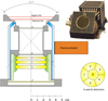 |
Fig. 1 Sketch (left) and photo (right) of the Electron Proton Helium INstrument (EPHIN). Bottom right: segmentation of solid state detectors A and B. |
2 Instrument description
The EPHIN (Müller-Mellin et al. 1995) is part of the Comprehensive Suprathermal and Energetic Particle Analyzer (COSTEP) suite on board SOHO, which was launched in December 1995 and orbits the Lagrangian point L1. Figure 1 shows a sketch and a photograph of the instrument, which consists of six solid-state detectors (SSD-A - SSD-F in Fig. 1) enclosed in a scintillator (G) that acts as an anticoincidence. The first two solid state detectors (SSDs) are segmented, as shown in the lower-right panel. The segmentation was introduced to improve the isotopic resolution and reduce the instrument’s acceptance for high fluxes. It achieves this by electrically and logically deactivating the outer ring segments of SSD-A and SSD-B, which the instrument automatically deactivates when the count rate in the inner segment of the first detector exceeds a threshold (see, e.g., Müller-Mellin et al. 1995).
Table A.1 in the appendix summarizes four electron, proton, and helium channels defined by particle penetration depth. Different thresholds in SSD-A discriminate between electrons, protons, and helium. In 1997 and 2017, electronic noise in SSD-E and SSD-D increased significantly. These detectors were excluded from the coincidence logic by switching the instrument into failure mode (FM) E and D on February 19, 1997 and October 4, 2017, respectively (see Kühl et al. 2020, for details). As a result, EPHIN was limited to three electron channels from 1997 to 2017 and to only two channels after 2017. The covered energy ranges of these two electron channels differ significantly. One channel collects the electrons that stop in SSD-B and the other collects the electrons that pass through SSD-B and do not reach SSD-F (Fig. 1). This results in a wide energy range, making the energy determination of incoming particles difficult.
Various datasets exist for the instrument (see, e.g., Kühl et al. 2020; Kühl & Heber 2019; Kühl et al. 2017, and references therein), with most implemented due to the loss of the two detectors. Up-to-date datasets are only available for ions. Here, we present novel electron flux data products derived from a thorough GEometry ANd Tracking (GEANT)-4 simulation of the instrument, including a detailed analysis of its data processing.
3 Data analysis
The EPHIN provides several datasets (for details see Kühl et al. 2020, and references therein). First, housekeeping data monitor the instrument health, including leakage currents, voltages, and temperatures. Second, coincidence counters separate the incoming particles according to detection thresholds. The counters sort the particles into different channels according to their species (i.e., electrons, protons, and helium ions) and energy, as discussed above. These data provide the instrument’s highest statistical significance, though particle separation and energy determination remain limited. Next, there is the pulse height analysis (PHA) dataset. When a valid coincidence is detected, the energy deposition in the SSDs-A to E is analyzed and stored. However, the time to digitize the energy loss is significantly longer (τd ~ 10 ms) than the time to determine a valid coincidence (τa ~ 3 μs). Consequently, not all particles that produce a valid coincidence can be analyzed for their exact energy loss in the detectors. (Sierks 1997). The PHA dataset provides the measured energy loss in SSD-A to E and allows for particle separation and high energy resolution. However, due to the limited transmission rate, this dataset provides only a statistical sample of the incoming particle distribution. To overcome this limitation, the instrument stores the total deposited energy for each PHA-analyzed particle in one of four histograms, based on its penetration depth. Since a software patch in 1998, this histogram uses only parallel coincidences, i.e., coincidences for which the segment numbers in SSD-A and B are the same. The new data product presented here uses data collected after this software patch; therefore, no data are available for 1995-1997. The histogram data lie between the two datasets described above and provide better statistics than the PHA data and improved energy determination than the coincidence counters. The temporal resolution was eight minutes from 1998 until March 2023. Due to the loss of two SSD in 1997 and 2017, the instrument was reprogrammed in March 2023 to obtain histograms only for particles that stop in the second detector, increasing the temporal resolution to one minute.
Using the histogram dataset for this data product allows us to provide channels at higher energies than would be possible using the PHA dataset. At higher energies, the low instrument response and the greater abundance of lower-energy particles make it unlikely that a high-energy particle is written to the PHA buffer before it fills with low-energy particles. In contrast, the histogram dataset stores every PHA-analyzed particle. Consequently, the higher- energy histogram channels are more likely to be filled than the corresponding PHA channels at the same energy. This partially compensates for the loss of the D and E detectors.
In this study, we systematically evaluate the histogram data for the first time. Using this dataset, we derive electron fluxes with significantly better energy resolution than previously published EPHIN-based results.
In the following, we describe the histogram data in detail (Sect. 3.1) and explain how we determine the electron response functions for the relevant histogram channels. Sect. 3.2 describes how we derive response factors from the electron response functions, accounting for their complex shapes and minimizing spectral dependence. These factors allow us to determine the particle flux in each channel from the corresponding count rates. In Sect. 3.3, we investigate the potential contamination of the electron channels caused by the automatic reduction of the instrument’s geometric factor during events with high particle fluxes and show how we correct this contamination. In Sect. 3.4, we demonstrate how ions contaminate electron channels, particularly those at higher energies. The final section (Sect. 3.5) summarizes the entire processing chain, from the raw histogram counts to the final electron flux in each channel.
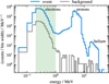 |
Fig. 2 Histograms recorded during a particle event on May 29, 2021 (blue) and the pre-event background (gray), each with an integration time of approximately 24 hours. The green area marks the range of histogram bins used in the data product. |
3.1 The histogram dataset
Each of the four histograms consists of 64 bins with widths that increase at higher energies (see, e.g., Sierks 1997). Table D.1 lists the energy channels for the first histogram, i.e., for particles stopping in SSD-B, where the sum of the energy deposited in SSD-A and SSD-B is recorded. With the loss of the SSDs-D and E, the total energy loss in the instrument is only available for particles stopping in SSD-B. Consequently, this histogram remains the only usable one, because the others are either empty or contain a mixture of particles stopping in SSD-C and particles penetrating SSD-C without reaching SSD-F, which we cannot disentangle.
The major difference from the coincidence and PHA datasets is that the histogram dataset is not based on particle separation by different thresholds in SSD-A (see Table A.1). Instead, the total energy loss for each penetration depth is stored in bins ranging from approximately 100 keV to several tens of MeV. Table D.1 lists the energy range and expected particle type for each histogram channel.
As an example, Fig. 2 shows the histogram of particles stopping in SSD-B during a particle event on May 29, 2021, alongside the corresponding pre-event background. The counts, normalized by the bin widths in MeV, are plotted as a function of the total energy loss in SSD-A and B. Both histograms are integrated over approximately 24 hours. The event histogram reveals three distinct populations, attributed to electrons, protons, and helium particles, whereas the background histogram primarily shows electrons. The green area indicates the range of histogram bins used in the data product presented here. This interval corresponds to the nominal channel energies of the histogram, i.e., the energies measured by the instrument. In contrast, the energy range given in the introduction refers to the primary energy of the particles that causes the measured energy losses in the instrument. Further details are provided in Sect. 3.2.
To determine the incident electron flux from the histogram count rates, we performed extensive Monte Carlo simulations using the GEANT-4 (Agostinelli et al. 2003) toolkit to calculate the response functions for the first 32 channels of the histogram and to identify possible contamination due to protons in these channels. This process involved refining an existing instrument model to more accurately reflect the logic and geometry of the actual instrument, as detailed in Hörlöck et al. (2026).
Following Sullivan (1971), the instrument response functions R(E) for an isotropic spherical particle source can be determined from simulations as follows:
 (1)
(1)
where n(E) is the simulated count rate at an energy E, N(E) denotes the number of simulated particles at this energy, and A is the surface area of the particle source. Valid coincidences are energy losses above the threshold in SSD-A and B with the segment in SSD-A equal to that in B (since the histogram only includes parallel incidences; see Section 2), no signal in SSD-C, and no anticoincidence G. These requirements are solely based on the instrument’s logic, i.e., particles meeting them are sorted into the first histogram by EPHIN.
We simulated 109 electrons emitted isotropically from a hemispherical source with a radius of 12 cm, covering the front of the instrument. We used a hemispherical source instead of a full 4π source to save computing time and storage. Because we considered only stopping particles, entries from the sides or the back of the instrument were rejected by the anti-coincidence logic, so this choice does not affect the resulting response function. The incident particles energies range from 0.1 to 30 MeV and follow a power-law distribution with spectral index γ = −1. The choice of index does not affect the determination of the instrument’s response, as it can be reweighted during postprocessing. However, γ = −1 is a convenient choice, as it yields an equal number of simulated particles per bin for logarithmic energy bins. Since the instrument provides no information on the angular distribution of the incident particles, we assumed isotropic flux within the viewing cone. Consequently, the calculated response functions are strictly valid only under this assumption.
Figure 3 shows the computed electron energy-dependent response functions, defined as the sum of the energy losses in detectors A and B (∆E = EA + EB) between the limits [(∆E)low, (∆E)up] ranging from [200, 250] keV to [700, 750] keV. We chose these ranges because Böhm et al. (2007) found significant electron responses in a similar investigation.
Figure 3 shows that electron response functions have long tails that extend to higher energies. This results from electron scattering within the detectors: an electron with sufficient kinetic energy to reach detector C scatters out of the field of view, depositing its energy in the instrument housing and being falsely identified as stopping in B. This characteristic complicates the determination of the channel’s effective energy, i.e., the expected energy at which the detected particle distribution peaks, since it strongly depends on the spectrum of the incoming particle (see, e.g., Oleynik 2021, and references therein). The arithmetic or geometric mean is often used to estimate the effective energy. However, this approach is only correct if the response is boxlike. To mitigate the dependence of channel effective energy on the incoming particle spectrum, we conducted a bow-tie analysis for each channel, as described in the following section.
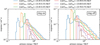 |
Fig. 3 Electron energy dependent response functions. We define these as the sums of the energy losses between a lower and an upper limit [(∆E)low, (∆E)up], ranging from [200, 250] to [700, 750] keV. Left: “Ring on” configuration. Right: “Ring off” configuration. |
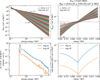 |
Fig. 4 Top left: power-law input spectra with a spectral index ranging from −6.0 to −1.5 in steps of 0.1. Bottom left: response function of the seventh histogram channel. Top right: channels response factors, calculated using Eq. (4), plotted against an energy interval around the channel’s nominal energy range. The effective energy Eeff and characteristic response RBT are indicated by dotted horizontal and vertical lines, respectively. Bottom right: total distance between the response factors (see text), with effective energy corresponding to the minimum of this distance. |
3.2 Bow-tie analysis
The bow-tie method aims to identify an effective energy and characteristic response factor for instrument channels that ideally remain constant across different incident particle spectra. This is particularly important for the electron channels, as their effective energy can vary significantly with the incoming particle spectrum due to the non-box-like shape of the electron response functions (see bottom-left panel of Fig. 4). This method was first introduced by Van Allen et al. (1974).
For an ideal, delta-peak-like response, Oleynik (2021) demonstrates that the characteristic response factor remains constant across different incident power-law spectra. However, for real instruments with non-box-like responses, the characteristic response deviates from a constant factor and depends on the choice of the simulated test spectrum, i.e., under the assumption of power-law spectra, the response factor depends on the spectral index. Next, we describe how we determined the pairs of characteristic response and effective energy for each electron channel.
As an example, we use the histogram channel ch7 (i.e., [(∆E)low, (∆E)up] = [350, 400] keV; Table D.1) to illustrate the method. First, we define a series of power-law test spectra F(E, γ) = A ∙ Eγ. We adapt spectral indices to the expected range of the actual particle spectra. Because the data product focuses primarily on Solar Energetic Particle (SEP) events, we chose a spectral range of γ = −6.0 to γ = −1.5 (see, e.g., Moses 1987; Dresing et al. 2020, and references to it), in steps of 0.1. This set of input spectra is shown in the top-left panel of Fig. 4. We multiply these spectra by the channel response function R(E) (bottom-left panel of Fig. 4). This yields the energy-dependent count rate, C(E, γ), as
 (2)
(2)
where ∆E is the response function bin width. We then sum over all energy bins Ei to obtain the total count rate of the channel,
 (3)
(3)
where n is the total number of bins in R(E). Next, we calculate a response factor Rchan representing the factor needed for the channel to recover the correct simulated differential flux per MeV, F(E, γ), from the calculated counts Cchan(γ):
 (4)
(4)
The top-right panel of Fig. 4 shows the response factors from Eq. (4) for this histogram channel, plotted as a function of energy E. Each curve corresponds to a different spectral index, γ. The combined shape of these curves resembles a bow tie, which gives the method its name. No single point exists where all the curves intersect, as would be the case for an instrument with an ideal narrow, box-like response. Therefore, we define the point at which the distance between the highest and lowest curves is minimal as the channel’s effective energy. We define the distance as
 (5)
(5)
where Γ = {γ0,..., γN} represents the set of spectral indices used (bottom-right panel of Fig. 4). We define the effective energy Eeff such that
 (6)
(6)
The characteristic response is defined as the average of the highest and lowest responses of all spectral indices, γ, at the energy Eeff:
 (7)
(7)
To account for response variation with different spectral indices, we take the distance between the lowest response, min(Rchan(Eeff, Γ)), and the highest response, max(Rchan(Eeff, Γ)), as the systematic uncertainty of the characteristic response. By definition, Eeff has no uncertainty, as its uncertainty is reflected in the characteristic response, RBT.
Using the same methodology, we computed the effective energies and characteristic responses for 15 electron channels, with effective energies ranging from approximately 300 keV to 1 MeV. Table E.1 lists the results. Each channel was computed twice: once under the “ring on” condition and once under the “ring off” condition, as shown in Fig. 5. The discontinuity observed in the characteristic response of the three highest channels arises because, in these channels, the energy width associated with the measured particle energy is twice that of the preceding channels (see Table D.1). Each channel has two characteristic responses, due to the instrument’s automatic ring switch mechanism (see Sect. 2). When the outer rings are turned off, the geometric factor of the histogram channels decreases by a factor of five. This can be seen by comparing the two response functions of the seventh histogram bin for the “ring on” and “ring off” states in the bottom-left panel of Fig. 4. This switching of the geometric factor would result in new effective energy and characteristic response pairs. However, to avoid a change in the channel energy during ring switching, we adopted the effective energy for the “ring on” state for the “ring off” state and determined only a new characteristic response. This increases systematic uncertainty because the channel response deviates more with the incident spectral index γ at that energy. This behavior is illustrated in the bottom right panel of Fig. 4, where the blue and orange curves show the evolution of the total distance between the response functions from the top-right panel, for the “ring on” and “ring off” states, respectively. This systematic uncertainty should not be interpreted in the strict sense. The calculated fluxes are not consistently over- or underestimated; rather, the error depends on the spectrum of the incoming particles. For very hard spectra, the flux is overestimated, whereas for very soft spectra, it is underestimated (see the top-right panel of Fig. 4).
 |
Fig. 5 Computed characteristic responses for E0 to E14 from Table E.1 for “ring on” and “ring off” conditions, in blue and orange, respectively. |
3.3 Ring-switch mechanism
One feature of EPHIN is the automatic reduction of the geometric factor during high-flux events (see instrument description in Sect. 2). For the coincidence channels, the geometric factor decreases by a factor of 25, since only the central segments of detectors A and B are used in this mode, whereas all particles incident within the instrument’s field of view are otherwise recorded. The blue curve in the top panel of Fig. 6 illustrates this effect on the E150 electron channel count rates. The time profiles were recorded during an interplanetary shock event (see Oliveira 2023). The drop in this count rate marks the moment the ring switches off (as indicated by the red and green shaded areas). This drop is expected because of the reduction in the geometric factor. The proton P4GM channel (orange curve), exhibits the opposite behavior. Its count rate increases when the ring is turned off and decreases when it is turned back on. The P4GM channel provides the count rate of low-energy protons for the central segments only. Therefore, its count rate should remain constant during ring switching if the proton flux does not change. Although moderate, gradual increases can be explained by an increased flux during the time of a “ring off” switching, the observed discontinuities, i.e., jump in fluxes, are an unexpected behavior. To better understand the cause of the additional counts during “ring off” times, the bottom panels of Fig. 6 show the energy deposition in the A detector plotted against the energy deposition in the B detector for all three AB coincidence channels (i.e., electrons, protons, and helium particles).
All entries below the A1 threshold are classified as electrons and are counted in the E150 coincidence channel. Entries between A1 and A4 are identified as protons and therefore counted in the P4 channel, while everything above A4 is classified as helium and counted in the H4 channel (see Table A.1).
During the “ring on” phase, the three main populations of electrons, protons, and helium are clearly visible. These populations are well-separated, with only minor contamination between the channels. However, during the “ring off” phase, additional clusters appear in both the electron and proton channels.
The population below the main proton track is most likely attributable to protons with energies similar to those of the main track. This interpretation is supported by the comparable energy distribution in SSD-B for both populations, as shown in the bottom-right panel of Fig. 6. In this panel, the energy spectra corresponding to the main track are shown in orange and red, matching the boxes in the bottom-middle panel, while the brown and violet curves represent the region below the main track.
The key difference between the protons of the main track and those of the lower population lies in their entry point: the latter enter the instrument through the outer ring of SSD-A and hit the middle segment of SSD-B. Since this ring is switched off, the energy deposition in SSD-A is not recorded, and these particles alone cannot trigger a valid coincidence. However, if such a proton arrives within the 2.4 μs coincidence window (Müller-Mellin et al. 1995) together with a low-energy ion that triggers the middle segment of SSD-A, the instrument generates a valid coincidence.
The slight relative enhancement of the brown distribution relative to the orange distribution at energies below 400 keV is attributed to electrons that can also coincide with low-energy protons. The population observed below the brown and violet boxes is most likely caused by electron-proton coincidences for SSD-B energies above 1 MeV and by electron-electron coincidences for energies below 1 MeV.
For the new electron data product, most of the proton contamination is removed, as indicated by the blue curved line in the lower-left and lower-right panels of Fig. 6. This line represents the highest energy value of the histogram used. However, electrons also form random coincidences with other electrons. These events cannot be distinguished from normal electron coincidences, i.e., electrons traversing the middle segment of SSD-A and stopping in the middle segment of SSD-B. Consequently, we underestimate the response for electrons when the ring is switched off and, as a result, the calculation yields fluxes that are too high.
To correct for this, we estimate the number of random coincidences caused by electrons entering through the outer ring of SSD-A using
 (8)
(8)
where nA represents the count rate caused by noise or particles that trigger only the middle segment of SSD-A (A0) without triggering SSD-B (A0B0). Since the instrument data does not directly provide this information, we approximate nA using the single-detector count rate, A0 (see Kühl et al. 2020, and references therein). This approximation is reasonable because, during an event, the count rate in A0 is more than 20 times higher than the count rate in the middle segment of SSD-B (B0); therefore, A0 ≈ A0B0. Similarly, nB represents the count rate in B0 caused by particles entering through the outer ring of detector A (B0A0). However, because the outer ring is electrically turned off, the instrument does not provide this information directly. Therefore, we estimate nB by multiplying the B0 count rate by 0.81. This factor arises from the ratio of the geometric factor for particles entering through the ring of detector A and hitting detector B to that for particles entering through any segment of detector A and hitting detector B. The quantity τ denotes the duration of the digital electronics’ coincidence window, where τ = 2.4μs. Thus, Eq. (8) becomes
 (9)
(9)
The approximation in Eq. (8) is based on the condition that the particle events follow a Poisson distribution and that nA,B ∙ τ << 1.
Equation (8) gives the number of random coincidences, distributed across all penetration depths. To estimate the number of random coincidences specifically for the AB penetration depth, we scale this value by the ratio of the counts in the AB coincidences (CAB) to the total coincidence counts (Call):
 (10)
(10)
Using Eq. (10), the fluxes in the histogram channels (Func) can be corrected as
 (11)
(11)
To test this correction method, we examined approximately 180 ring-switch events over the entire mission duration. For each event, we analyzed the declining phase of the particle flux and calculated the ratio of the eight-minute averaged flux immediately before the ring was turned on to that immediately after. The declining phase was chosen because only small, gradual flux variations occur during this period, in contrast to the flux increase at event onset, when the ring is typically switched off. Without correction, these ratios have a mean of approximately 1.5. Applying the correction reduces the mean ratio to approximately 1.0, indicating that the discontinuities associated with ring switching can, on average, be fully corrected.
However, for some events, this method results in overcorrection, producing small or even negative fluxes. This typically occurs during events with fluxes high enough to saturate the A detector because of its dead time. Consequently, we exclude fluxes from the data product for events in which the correction factor ρAB equals or exceeds the total AB coincidence count, CAB. For these events, we report only the count rates.
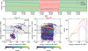 |
Fig. 6 Top: count rates of the E150 and the P4GM coincidence counters during an automatic ring switch event of the instrument. Bottom left and middle: energy deposition in the A detector versus B detector during the “ring off” and “ring on” periods, respectively. The time intervals are highlighted in the top panel, with the “ring on” period in green and the “ring off” period in red. The blue curved line shows the highest measured energy used in this data product. The horizontal lines labeled with A1 and A4 indicate the energy thresholds used by the instrument to distinguish between protons, electrons, and helium particles. Bottom right panel: energy-loss distribution in SSD-B of all entries inside the corresponding boxes in the middle panel. |
3.4 Contamination
One disadvantage of using the histogram dataset is that it considers only the lowest detection thresholds of SSD-A, rather than all five thresholds. These thresholds normally identify and distinguish between electrons, protons, and helium particles. However, because the histogram dataset combines all particle species into a single distribution, the thresholds cannot be applied individually. As a result, particle identification relies solely on the total energy loss in the two detectors, which can lead to misidentification. Consequently, the electron channels can be contaminated by ions in some events.
Fig. 7 shows an example event in which contamination of the higher electron channels occurs. The left panel shows the dynamic spectrum of the event, with channel energy plotted against time. The entries are color-coded according to the counts per MeV accumulated over eight-minute intervals. Dashed and dotted lines indicate the two integration intervals. During the dashed interval (I), the channels above 1 MeV are barely populated. In contrast, during the later phase of the event, a population of particles appears above 1.5 MeV and gradually extends into the lower-energy channels. These entries cannot be caused by electrons and must be ions, as the electron response at these energies is negligible. The right panel shows the integrated spectra for the dashed and dotted time intervals in blue and orange, respectively (gray points also correspond to the dotted interval).
The dashed interval (I) lies outside the ion cloud; therefore, the integrated spectrum exhibits the expected shape, following a power-law function with a negative spectral index. In contrast, the dotted interval (II) falls within the ion cloud, resulting in a spectrum that deviates from the expected shape. Here, the spectrum above 800 keV shows a positive slope. This additional count rate, which is then converted to particle flux, is caused by ion contamination. The contamination is predominantly caused by protons, which are generally the most abundant. However, the channels can also be contaminated by helium and heavier ions (see Appendix C).
Depending on the event, contamination can extend into the lower-energy channels. In this data product, a flag indicates, for each timestamp, the highest channel that is considered to be uncontaminated. Fig. 7 illustrates this: the orange stars indicate uncontaminated channels, while the gray channels are likely contaminated by ions. Because the highest uncontaminated channel reported may fluctuate statistically, we used the minimum flag value over the entire integration period of the spectrum. This example shows that the flag provides a very conservative estimate of the contaminated channels, ensuring that users can be reasonably confident that only channels with negligible contamination are included in their analysis. We include all data used to generate the flag in the data product. This allows users to reproduce the flag and adapt it to their specific problem if necessary. Appendix C describes how we generated this contamination flag.
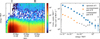 |
Fig. 7 Example event from 29, May 2021 illustrating ion contamination in the higher electron channels. Left: dynamic spectrum of the event. Two time intervals (I) and (II) are indicated by dotted and dashed lines, respectively. Right: corresponding energy spectra. |
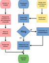 |
Fig. 8 Flow chart of the processing chain from raw data to final electron flux. |
3.5 Summary of the processing chain
Next, we provide an overview of all steps included in the processing chain, from raw data to the final electron fluxes. The processing chain consists of three main branches, illustrated in Fig. 8 in red, blue, and yellow.
The modeling branch (red) determines the response factors for each electron channel. It begins by modeling the instrument’s geometry and simulating its response to electrons. We performed the simulations using the GEANT-4 toolkit. Hörlöck et al. (2026) provide a detailed description of the instrument model. The resulting response functions were then used to perform a bow-tie analysis to determine the response factors and effective energies for each electron channel, as described in Sect. 3.2.
The blue branch represents the processing chain that starts with the raw histogram counts and leads to the final electron fluxes. First, we correct the raw histogram counts for dead time effects, as described in Appendix B. This correction method depends on the instrument’s coincidence counters, which themselves must also be corrected for dead time effects (yellow branch). Appendix B.1 describes the correction of the single and coincidence counters. We then checked each data point to determine whether the outer segments of detectors A and B were switched off. If the ring was switched off, we corrected the data for possible contamination, as described in Sect. 3.3. We then checked the data for potential ion contamination and generated a contamination flag, as described in Appendix C. Finally, we applied the response factors from the red branch to determine the final electron fluxes for each electron channel.
Table 1 summarizes the key characteristics of the existing electron data product (Level 2 electron data) and the newly developed data product (histogram electron data), highlighting the improvements of the present work over previous data.
4 Validation and comparison
To test and validate our data product, we compared it with the instruments SolO / Electron Proton Telescope (EPT), SolO / High Energy Telescope (HET) (Rodríguez-Pacheco et al. 2020), WIND / Three-Dimensional Plasma and Energetic Particle Instrument (3DP) (Lin et al. 1995), and Advanced Composition Explorer (ACE) / Electron Proton Alpha Monitor (EPAM) (Gold et al. 1998). Comparison with the instruments on SolO was possible because, during the Earth gravity assist maneuvers around November 2021, SolO came close to the spacecrafts at L1. The left panel of Fig. 9 shows the flux time profile of the five instruments from December 4 until December 9, 2021, when the spacecraft were still close together. The green profile represents the EPAM DE2 channel, which corresponds to deflected electrons with an energy of about 74 keV. The electron flux between 92 and 102 keV, measured by the EPT instrument, is plotted in blue. The Ch6 channel of the 3DP instrument measures electrons at around 308 keV and is shown in red. The first electron channel of HET and EPHIN’s E1 channel (328 keV) are shown in brown and orange, respectively. All shown fluxes are sector-averaged, except for the EPHIN flux, since EPHIN has only one viewing direction1.
The plot shows three electron events during this period. To compare the instruments, we selected the second event, which took place between December 5 and 6, and integrated the particle spectrum for each instrument. The integration intervals for the spectrum and the pre-event background are shown in green and gray, respectively. We selected this event because it did not show a spectral break between several tens of keV and approximately 1 MeV. This allowed us to include the lower-energy channels of the instruments in the fit method. This was necessary because 3DP, EPAM, and EPT have a relatively high background, and in this event the entries in the higher channels are indistinguishable from the background. This clearly demonstrates the benefits of an active anti-coincidence, as in EPHIN, because the background level is orders of magnitude smaller, making the instrument more sensitive to small events.
The middle panel of Fig. 9 shows the integrated energy spectra of all five instruments on a double-logarithmic scale. To allow a better comparison of the instruments, we scaled the spectrum by a factor of E3∙5 in the right panel, where E is the effective energy of the channels in MeV. This makes it possible to display the y-axis linearly. We subtracted the pre-event background from each spectrum.
When sector data were available, we did not use sector-averaged instrument data for the energy spectra to better account for the anisotropies in particle flux. The measured flux in the EPT north, south, and antisun telescopes is roughly equal, whereas the flux in the Sun telescope is about three times higher, indicating that EPT observes an anisotropic electron flux during this event. To avoid overloading the graph, we plotted only the average value of the sectors in the 3DP data. The range between the highest and lowest sector is shaded red. Two sectors exhibited unphysically high fluxes in only two energy channels. The remaining energy channels in these sectors were consistent with those in the other sectors. Because the exact functioning of the instrument is unknown, we excluded these sectors from the analysis. The measured 3DP fluxes fall between those of the EPT Sun telescope and the other EPT sectors. The plotted EPAM energy spectrum shows the sector-averaged fluxes of the instrument, as flux measurements for individual sectors were not available. The EPAM measurements are consistent with those of 3DP. The fluxes measured by EPHIN are consistent with those of EPT, except for the Sun direction. The outer rings of the detectors were not switched off during the integration interval of the spectrum. A possible explanation for the deviation relative to the EPT Sun telescope is that an anisotropic electron beam hit the EPT Sun telescope but not EPHIN, due to their spatial distance or because they were in different flux ropes. Compared with 3DP and EPAM the fluxes of EPHIN are approximately a factor of two lower. However, the measurements are also consistent with those of the lowest electron channel of HET, which is shown with stars of different colors for each of the four sector telescopes. We did not include the higher channels because they did not rise above the background.
Furthermore, we performed simple power-law (y = a ∙ Eγ) fits to all datasets except the 3DP measurements. Because these data do not provide uncertainties, we fit a linear function (y = γ ∙ E + a) to the logarithmic data to avoid the low-energy channels being weighted too strongly. The resulting spectral indices are listed in the legend of Fig. 9. All spectral indices are consistent within uncertainties, with the exception of the EPT Sun telescope, which measured a somewhat harder spectrum. This deviation may also be caused by the previously mentioned electron beam.
This comparison demonstrates that this new data product produces reliable measurements, as the EPHIN and EPT observations agree within the uncertainties. The measurements from 3DP and EPAM lie between those of EPHIN and three of the EPT telescopes. However, the sectors covered by 3DP do not cover the span between the EPT telescopes. This does not necessarily contradict the other instruments, as the connection of 3DP to the event could be different. A more detailed assessment would require an analysis of the magnetic field and solar wind plasma data. Such an analysis is outside the scope of this work. In a future study, we plan to present a systematic comparison based on multiple events, including the instruments used here, as well as STEREO / Solar Electron Proton Telescope (SEPT) (Kaiser et al. 2008).
In a further comparison, we compared the new data product with previously published EPHIN data. Because published event spectra from EPHIN are scarce, we compared our results with the Jovian electron spectrum published by Kühl et al. (2013). Fig. 10 illustrates this spectrum. It was averaged over seven two-hour time intervals, with good connection to Jupiter, in 2007 and 2008. We excluded the two highest channels from the fit because they were likely contaminated by ions. It should be noted that these channels were not flagged as contaminated because no significant entries were recorded in the proton-proxy channels. However, these channels may still be contaminated because the electron response is very small here (see Fig. 5), and thus contributions from ions strongly affect the calculated flux. This also implies that the contamination flag is reliable for SEP events, but not for the background.
The two spectra differ quite significantly. First, the spectrum determined by Kühl et al. (2013) includes higher and lower energies. This is because their analysis used the PHA dataset without restrictions on the angle of incidence and included coincidences for particles hitting the ABC and ABCD detectors. In contrast, the data product presented here is restricted to particles with parallel incidence and to AB coincidences only. The most significant difference between the spectra is that the previously published spectrum exhibits a spectral break at approximately 500 keV, which we cannot reproduce with our new data product. The authors also noted that the spectral break requires further investigation, as it could arise from either instrumental or transport effects (see page 4, Chap. 6 in Kühl et al. 2013). Using the new data product, we can now confirm that this feature was caused by not accounting for the complex shape of the electron response functions. At higher energies, both spectra agree in absolute flux and slope. From the fit, we obtain a spectral index of γ = −1.36. This value lies slightly outside the initially selected γ range for the bow-tie analysis (see Sect. 3.2). However, extending the bow-tie index range dis-proportionally increases the uncertainty, as the data product is primarily geared toward SEP events. We also evaluated the spectrum using the response factors for a fixed spectral index of γ = −1.3. The resulting flux differences are below 10% for all channels except for the two lowest channels, where the difference is below 30%. Nevertheless, even when these differences are taken into account, the conclusion regarding the spectral shape remains unchanged. These results also demonstrate that no further quiet-time analyses should be performed using this data product.
Key characteristics of existing and new electron data products.
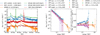 |
Fig. 9 Left: flux time profiles measured by EPT (blue), HET (brown), EPHIN (orange), EPAM (green), and 3DP (red) during the 2021 Earth gravity-assist maneuver of SolO. Middle: integrated spectrum of all five instruments. The integration background intervals are marked in the left panel in green and gray, respectively. 3DP channels with unphysically high fluxes are plotted as red open diamonds. Right: integrated spectrum on a linear scale (fluxes multiplied by E3.5). |
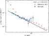 |
Fig. 10 Spectrum of Jovian electrons averaged over seven time intervals with good connection to Jupiter in 2007 and 2008. Red crosses indicate the spectrum determined by Kühl et al. (2013), while blue dots represent the spectrum obtained with our new data product. The black line represents a power-law fit to the blue data points; the solid line indicates the data points used for the fit. |
5 Summary and conclusions
We developed a new data product for SOHO/EPHIN, providing 15 electron channels covering energies from approximately 300 keV to 1 MeV. This data product is based on the instrument’s onboard histograms, enabling the inclusion of higher-energy channels than would be possible using the PHA dataset. As a result, the loss of the D and E detectors can be partially compensated. Using GEANT4 simulations, we determined the response function for each channel. Additionally, we derived effective energies and optimal response values - less dependent on the shape of the incident particle spectrum - using a bow-tie analysis.
We demonstrate that the instrument’s adaptive geometric factor (ring switch) can lead to contamination in all coincidence data during periods when the outer ring segments of detectors A and B are switched off, as particles crossing the ring segments leave a signal in the analog chain coincident with noise or with particles detected in the central detector segment during high-flux conditions. Furthermore, we introduce a method to correct for this effect in the channels included in this data product.
We also show that the data product is susceptible to ion contamination, primarily because particle separation in the histograms is based solely on the total energy loss rather than on energy losses in each detector. To address this, we introduce a flag to identify contaminated channels during periods of significant ion contamination and provide proxy channels that allow users to estimate the level of ion contamination.
However, the contamination flag is only reliable during SEP events, due to the relatively small electron response in the higher channels and the low count statistics of the electron background during quiet times. Furthermore, due to the chosen range of spectral indices used in the bow-tie analysis (see Sect. 3.2), this data product is specifically optimized for SEP events. As discussed in Sect. 4, the provided flux values during quiet times can exhibit large offsets that are not captured by the quoted uncertainties. Consequently, this data product should be used exclusively for studies of SEP events. Finally, it should be noted that the derived responses, and thus the provided flux values, implicitly assume that the incident particles are isotropic.
To validate the data product, we performed a comparison with SolO / EPT, SolO / HET, ACE / EPAM, and WIND / 3DP for one event during the Earth gravity assist maneuver of SolO. This comparison demonstrates that the measurements of EPHIN, HET, and three sectors of EPT agree within the uncertainties. However, the Sun telescope of EPT measured fluxes approximately three times higher, which we attribute to an anisotropic feature of the event.
In addition, we compared the new data product with previously published data for Jovian electrons from Kühl et al. (2013). We show that the spectral break reported in that study was most likely caused by incorrect handling of the instrument data.
With this new data product, it is now possible to extend the energy spectra obtained from instruments such as EPT, EPAM, and 3DP, enabling investigations of SEE spectra up to energies of 1 MeV. Moreover, thanks to SOHO’s long operational duration, this data product provides continuous coverage since 1998, offering a valuable resource for long-term studies and a significant contribution to the scientific community.
Data availability
An archive of this dataset, along with a description of the file structure, is available via Zenodo at https://doi.org/10.5281/zenodo.18225156. This archive will be updated annually. In addition, daily files can be accessed at http://ulysses.physik.uni-kiel.de/costep/level3/hist_electrons/.
Acknowledgements
The SOHO/EPHIN project is supported under Grant 50 OC 2302 by the German Bundesministerium für Wirtschaft through the Deutsches Zentrum für Luft- und Raumfahrt (DLR), Solar Orbiter/EPT is supported under Grant 50 OT 2002. This research benefited from funding provided by the European Union’s Horizon 2020 research and innovation program under grant agreement No. 101004159 (SERPENTINE), which has now concluded.
References
- Agostinelli, S., Allison, J., Amako, K., et al. 2003, Nucl. Instrum. Methods Phys. Res. A, 506, 250 [Google Scholar]
- Böhm, E., Kharytonov, A., & Wimmer-Schweingruber, R. F. 2007, A&A, 473, 673 [NASA ADS] [CrossRef] [EDP Sciences] [Google Scholar]
- Bécares, V., & Blázquez, J. 2012, Sci. Technol. Nucl. Install., 2012, 1 [CrossRef] [Google Scholar]
- Dresing, N., Gómez-Herrero, R., Heber, B., et al. 2014, A&A, 567, A27 [NASA ADS] [CrossRef] [EDP Sciences] [Google Scholar]
- Dresing, N., Effenberger, F., Gómez-Herrero, R., et al. 2020, ApJ, 889, 143 [NASA ADS] [CrossRef] [Google Scholar]
- Dresing, N., Rodríguez-García, L., Jebaraj, I. C., et al. 2023, A&A, 674, A105 [NASA ADS] [CrossRef] [EDP Sciences] [Google Scholar]
- Dresing, N., Yli-Laurila, A., Valkila, S., et al. 2024, A&A, 687, A72 [NASA ADS] [CrossRef] [EDP Sciences] [Google Scholar]
- Fox, N. J., Velli, M. C., Bale, S. D., et al. 2016, Space Sci. Rev., 204, 7 [Google Scholar]
- Gold, R. E., Krimigis, S. M., Hawkins, S. E. I., et al. 1998, Space Sci. Rev., 86, 541 [NASA ADS] [CrossRef] [Google Scholar]
- Hörlöck, M., Heber, B., Jensen, S., Kühl, P., & Sierks, H. 2026, Earth Space Sci., 13, 13 [Google Scholar]
- Kaiser, M. L., Kucera, T. A., Davila, J. M., et al. 2008, Space Sci. Rev., 136, 5 [Google Scholar]
- Kühl, P., & Heber, B. 2019, Space Weather, 17, 84 [CrossRef] [Google Scholar]
- Kühl, P., Dressing, N., Dunzlaff, P., Effenberger, F., et al. 2013, International Cosmic Ray Conference [Google Scholar]
- Kühl, P., Dresing, N., Heber, B., & Klassen, A. 2017, Sol. Phys., 292, 10 [Google Scholar]
- Kühl, P., Heber, B., Gómez-Herrero, R., et al. 2020, J. Space Weather Space Climate, 10, 53 [CrossRef] [EDP Sciences] [Google Scholar]
- Lin, R. P., Anderson, K. A., Ashford, S., et al. 1995, Space Sci. Rev., 71, 125 [CrossRef] [Google Scholar]
- Moses, D. 1987, ApJ, 313, 471 [Google Scholar]
- Müller, D., St Cyr, O. C., Zouganelis, I., et al. 2020, A&A, 642, A1 [Google Scholar]
- Müller-Mellin, R., Kunow, H., Fleißner, V., et al. 1995, Sol. Phys., 162, 483 [Google Scholar]
- Oleynik, P. 2021, PhD thesis, University of Turku, Finland [Google Scholar]
- Oliveira, D. M. 2023, Front. Astron. Space Sci., 10, 1240323 [Google Scholar]
- Raouafi, N. E., Matteini, L., Squire, J., et al. 2023, Space Sci. Rev., 219, 8 [NASA ADS] [CrossRef] [Google Scholar]
- Rodríguez-Pacheco, J., Wimmer-Schweingruber, R. F., Mason, G. M., et al. 2020, A&A, 642, A7 [Google Scholar]
- Rodríguez-García, L., Gómez-Herrero, R., Dresing, N., et al. 2025, A&A, 694, A64 [NASA ADS] [CrossRef] [EDP Sciences] [Google Scholar]
- Sierks, H. 1997, PhD thesis, Christian-Albrechts-University, Germany [Google Scholar]
- Sullivan, J. 1971, Nucl. Instrum. Methods, 95, 5 [Google Scholar]
- Van Allen, J. A., Baker, D. N., Randall, B. A., & Sentman, D. D. 1974, J. Geophys. Res., 79, 3559 [Google Scholar]
Appendix A Detailed instrument logic
Tab. A.1 shows the expected particle species, the name, the nominal energy range and the logical condition for each coincidence channel of the instrument. The coincidence logic specifies, for each coincidence, which detector thresholds must be exceeded and which must not (the latter indicated by letters with an overline).
Appendix B Dead time
The digital signal chain for pulse height analysis of a particle requires approximately 10 to 15 milliseconds. This results in dead time effects for the pulse height analysis during events with higher particle fluxes. These effects must be corrected to determine the true particle fluxes. To quantify the dead time of the PHA chain, we used in-flight data from 1999 to 2023 and calculated the ratios between the total number of histogram entries and the corresponding coincidence counters. This ratio is shown in the left panel of Fig. B.1 as function of the total stopping coincidence counts rate. Low and high count rates on the abscissa correspond to low and high flux rates, respectively. The number of entries in each bin is color-coded, as indicated by the color bar on the right side of the figure. The plot features two curves: The lower curve represents the ratios for the instrument in the "ring on" state, starting at a ratio of approximately 0.2 and decreasing at a count rate of around 25 counts per second. The upper curve, corresponding to the "ring off” state of the instrument, begins at a ratio of 1 and starts to decline at approximately 5 counts per second. The smaller ratio of the "ring on" states compared to the "ring off" states can be attributed to the fact that the on-board histograms only collect the particle events with parallel trajectories. This means that a particle must enter the instrument through segments with matching numbers in both the A and B detectors. In contrast the coincidence counters capture particles with arbitrary trajectories, constrained only by the viewing cone. Consequently, the geometric factor of the coincidence counters is about five times higher than that of the on-board histograms. However during the "ring off" state only particles entering through the center segments are registered, resulting in both the on-board histograms and the coincidence counters having the same geometric factors.
The dependency of the ratio on the count rate is determined by the dead time of the digital processing chain. To analyze the data, slices were made along the x-axis and, for each slice, the mean value and standard deviation of the distribution were determined. The right panel of Fig. B.1 shows these mean values plotted against stopping coincidence counts, with the error bars representing the standard deviation of each distribution. We used the correlation for a non-paralyzable dead time to fit these mean values. A non-paralyzable dead time means that the dead time is not extended if a particle arrives during the dead time of a previous event, for details see Bécares & Blázquez (2012):
 (B.1)
(B.1)
Here, N represents the true number of particles hitting the detector (in our case the coincidence counts), M is the number of particles the detector actually can resolve(in our case the histogram counts) and τ is the time constant of the dead time.
The "ring on" and "ring off" states were fitted individually. The fits also included a scaling parameter a which is about unity for "ring off" and approximately 0.2 for "ring on" due to the difference in geometry factor explained above. The resulting fits are shown as black lines in Fig. B.1. From the fits, we obtain a time constant of τ = 6.67 ms for the "ring on" state and τ = 8.59 ms for the "ring off" state. This means that the time constants differ depending on the operational mode ("ring on" or "ring off") of the instrument. This can be understood by the way the onboard software analyzes the energy losses of the incident particles (see Sierks (1997) and references therein). By applying these time constants, we can scale the entries in the histogram to reflect the actual number of particles that hit the detectors with:
 (B.2)
(B.2)
For N, we use the sum of all coincidence counters for stopping coincidences. These counters were also corrected for dead time effects, making them a reliable representation of the true number of particles reaching the instrument. The correction of the coincidence counters will be explained in Sec. B.1.
B.1 Dead time of single and coincidence counter
The dead time of the single counters is dominated by the time constant of the discriminator τd in the analog signal chain of each detector. Its task is to determine whether the particle’s charge pulse exceeds the detector’s threshold. The time constant of the discriminator is defined by the time it takes for the charge pulse to drop below a certain threshold. The exact time depends on the height of the charge pulse, i.e., on the energy of the incoming particle, but on average it is about τd = 5 μs. However, in contrast to the dead time of the PHA chain, this dead time is paralyzable. This means that if another particle hits the detector during the 5 μs time interval of the discriminator, the charge pulses of the particles are superimposed, thereby extending the discriminator’s dead time.
We built a simulation model that mimics this discriminator logic. When a particle event triggers the discriminator, its state is set to one, a counter is incremented, and a time window of τd = 5 μs is opened. After this time the discriminator state is reset to zero. However, if another particle event triggers the discriminator within τd, the time window τd is extended by 5 μs, and the counter is not incremented. To determine the expected counts M for a given number of particle events, we divided one second into 107 time steps. For each step, we draw from a Poisson distribution to decide whether the discriminator is triggered by a particle event. The mean value λ of the distribution is determined by the number of particle events N and the step size ∆t as follows:
 (B.3)
(B.3)
The results of this simulation are shown in Fig. B.2. The expected count rate M is plotted as a function of the rate of true particle events M. The black line represents the polynomial fit to the simulated data. This fit can be used to correct for the detector dead time by inverting the function, thereby obtaining the true number of particle events N from the measured count rate M.
To correct the coincidence counter, we built a simplified model of the instrument’s coincidence logic. In this model, only the A detector is considered, since it dominates the dead time of the coincidence channels. This is because it is located at the front of the instrument and is therefore exposed to the highest particle flux. Furthermore, its noise level is significantly higher than that of the other detectors. The dead time of the coincidence channels is determined by the coincidence time window τc. During this interval, the instrument waits for all detectors to respond to the incoming particle. After the time window has elapsed, the instrument decides whether the particle event constitutes a valid coincidence. However, if another particle event occurs in a different segment of the A detector during this interval, this event is not valid and therefore not counted. Consequently, this mechanism also contributes to the dead time of the coincidence channels. Our model replicates this behavior. Therefore, we use six of the previously described discriminator models, corresponding to the six segments of the A detector. As before, we draw from a Poisson distribution to decide whether a segment is triggered. This event then starts the discriminator time window τd. If the triggered segment is the first one, a coincidence time window τc = 3 μs is opened as well. After τc the window is closed and the coincidence counter is incremented. However, if another segment is triggered within 2.4 μs, this coincidence is vetoed and therefore not counted. It should be noted, that this 2.4 μs is the actual duration of the coincidence window, i.e.,during that time the instruments listens for detector signals. However, resetting the electronic chain also takes time and therefore the instrument is only ready for further events after τc = 3 μs.
Predefined coincidence channels used by EPHIN.
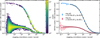 |
Fig. B.1 Left: A two-dimensional histogram showing the ratio between the counts in the first histogram and the coincidence counters for particles stopping in the B detector. The bottom curve represents data taken during the "ring on" state, while the top curve corresponds to the "ring off" state. Right: Mean values of slices taken from the 2D histogram shown in the left panel. The error bars indicate the standard deviation within each slice. |
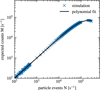 |
Fig. B.2 Simulation results for the single detector dead time. This plot shows the expected count rate M for a given rate of particle events N. The data points were fitted with a polynomial function, which is shown with the black line. |
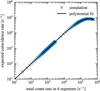 |
Fig. B.3 Simulation results for the dead time of the coincidence channels. Plotted is the expected coincidence rate against the total count rate in all six segments of the A detector. The black line represents a polynomial fit to the data. |
The results of this simulation are shown in Fig. B.3. The figure displays the expected coincidence rate as a function of the total count rate across all six segments. The black line represents a polynomial fit to the simulation data. This fit can then be used to correct for the dead time of the coincidence counter.
Appendix C Determination of the contamination flag
The data product provides both a flag and dedicated channels (proton proxy) that indicate the current level of proton contamination in the electron channels. Fig. C.1 shows the GEANT-4 simulation results for electrons (0.1-30 MeV), protons (0.1 −500 MeV) and helium particles (0.1-500 MeV). The flux in each bin is plotted as a function of the total energy deposited in the A and B detectors. The binning reflects the actual binning of the instrument’s first histogram. The spectra of the incident particles follow a power-law with a spectral index of γ = −3, which serves as a good approximation for typical event spectra.
As can be seen, at energies around 2 MeV and above the main contribution to the channel fluxes comes from protons (blue curve), and at even higher energies, from helium particles (orange curve). Furthermore the proton flux at these energies is of the same order of magnitude as the proton flux at the lower energies, where the electron channels are located (green curve). Therefore, we can use these channels (ch24, ch25, ch26) to estimate the proton contamination in the electron channels. These channels are also sensitive for helium particles and can therefore be used to indicate helium contamination. However, the contribution of the particle species can not be disentangled and since protons are in general more abundant in SEP events, we are mainly considering protons.
The flag provided in this data product indicates for every time stamp the highest channel that is considered as uncontaminated. The flag is determined as follows: First, we divide the 15 electron channels into groups of three, such that the first group consists of channels E0, E1 and E2, the second group of channels E3, E4 and E5, and so on. The total count rate of each group is then divided by the total count rate of the proxy channels. Groups of channels are used instead of individual channels to reduce statistical fluctuations. A group of channels is considered as contaminated, when the calculated ratio gets below 2.0. This is a empirical threshold based on the investigation of about 60 events.
It should be noted that the described method provides only a rough estimation for the contamination of the electron channels. However, empirical studies have shown that this flag gives a reliable and conservative indication of contamination.
Appendix D EPHIN histogram energy ranges
Tab. D.1 lists the lower and upper energy thresholds for the different histogram channels of the instrument. It should be noted that these energies represent the measured energy losses in the detectors, which can differ from the actual primary energy of the incoming particle (for further details, see Sec. 3.2). The table also includes the expected particle types as given by Sierks (1997).
Appendix E Histogram electron channels
Tab. E.1 lists all electron channels defined in this data product. For each channel, the corresponding histogram channel from which it was derived is given, along with the effective energy and characteristic response. The latter is provided for both the "ring on" and "ring off" states.
Energy bands of the different histogram channels.
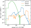 |
Fig. C.1 Results of a GEANT-4 simulation for electrons, protons and helium particles. Shown is the particle flux as a function of the total energy deposited in the A and B detectors. |
Effective energies and characteristic responses for the electron channels of the histogram data.
All Tables
Effective energies and characteristic responses for the electron channels of the histogram data.
All Figures
|
Fig. 1 Sketch (left) and photo (right) of the Electron Proton Helium INstrument (EPHIN). Bottom right: segmentation of solid state detectors A and B. |
| In the text | |
|
Fig. 2 Histograms recorded during a particle event on May 29, 2021 (blue) and the pre-event background (gray), each with an integration time of approximately 24 hours. The green area marks the range of histogram bins used in the data product. |
| In the text | |
|
Fig. 3 Electron energy dependent response functions. We define these as the sums of the energy losses between a lower and an upper limit [(∆E)low, (∆E)up], ranging from [200, 250] to [700, 750] keV. Left: “Ring on” configuration. Right: “Ring off” configuration. |
| In the text | |
|
Fig. 4 Top left: power-law input spectra with a spectral index ranging from −6.0 to −1.5 in steps of 0.1. Bottom left: response function of the seventh histogram channel. Top right: channels response factors, calculated using Eq. (4), plotted against an energy interval around the channel’s nominal energy range. The effective energy Eeff and characteristic response RBT are indicated by dotted horizontal and vertical lines, respectively. Bottom right: total distance between the response factors (see text), with effective energy corresponding to the minimum of this distance. |
| In the text | |
|
Fig. 5 Computed characteristic responses for E0 to E14 from Table E.1 for “ring on” and “ring off” conditions, in blue and orange, respectively. |
| In the text | |
|
Fig. 6 Top: count rates of the E150 and the P4GM coincidence counters during an automatic ring switch event of the instrument. Bottom left and middle: energy deposition in the A detector versus B detector during the “ring off” and “ring on” periods, respectively. The time intervals are highlighted in the top panel, with the “ring on” period in green and the “ring off” period in red. The blue curved line shows the highest measured energy used in this data product. The horizontal lines labeled with A1 and A4 indicate the energy thresholds used by the instrument to distinguish between protons, electrons, and helium particles. Bottom right panel: energy-loss distribution in SSD-B of all entries inside the corresponding boxes in the middle panel. |
| In the text | |
|
Fig. 7 Example event from 29, May 2021 illustrating ion contamination in the higher electron channels. Left: dynamic spectrum of the event. Two time intervals (I) and (II) are indicated by dotted and dashed lines, respectively. Right: corresponding energy spectra. |
| In the text | |
|
Fig. 8 Flow chart of the processing chain from raw data to final electron flux. |
| In the text | |
|
Fig. 9 Left: flux time profiles measured by EPT (blue), HET (brown), EPHIN (orange), EPAM (green), and 3DP (red) during the 2021 Earth gravity-assist maneuver of SolO. Middle: integrated spectrum of all five instruments. The integration background intervals are marked in the left panel in green and gray, respectively. 3DP channels with unphysically high fluxes are plotted as red open diamonds. Right: integrated spectrum on a linear scale (fluxes multiplied by E3.5). |
| In the text | |
|
Fig. 10 Spectrum of Jovian electrons averaged over seven time intervals with good connection to Jupiter in 2007 and 2008. Red crosses indicate the spectrum determined by Kühl et al. (2013), while blue dots represent the spectrum obtained with our new data product. The black line represents a power-law fit to the blue data points; the solid line indicates the data points used for the fit. |
| In the text | |
|
Fig. B.1 Left: A two-dimensional histogram showing the ratio between the counts in the first histogram and the coincidence counters for particles stopping in the B detector. The bottom curve represents data taken during the "ring on" state, while the top curve corresponds to the "ring off" state. Right: Mean values of slices taken from the 2D histogram shown in the left panel. The error bars indicate the standard deviation within each slice. |
| In the text | |
|
Fig. B.2 Simulation results for the single detector dead time. This plot shows the expected count rate M for a given rate of particle events N. The data points were fitted with a polynomial function, which is shown with the black line. |
| In the text | |
|
Fig. B.3 Simulation results for the dead time of the coincidence channels. Plotted is the expected coincidence rate against the total count rate in all six segments of the A detector. The black line represents a polynomial fit to the data. |
| In the text | |
|
Fig. C.1 Results of a GEANT-4 simulation for electrons, protons and helium particles. Shown is the particle flux as a function of the total energy deposited in the A and B detectors. |
| In the text | |
Current usage metrics show cumulative count of Article Views (full-text article views including HTML views, PDF and ePub downloads, according to the available data) and Abstracts Views on Vision4Press platform.
Data correspond to usage on the plateform after 2015. The current usage metrics is available 48-96 hours after online publication and is updated daily on week days.
Initial download of the metrics may take a while.