| Issue |
A&A
Volume 708, April 2026
|
|
|---|---|---|
| Article Number | A84 | |
| Number of page(s) | 24 | |
| Section | Planets, planetary systems, and small bodies | |
| DOI | https://doi.org/10.1051/0004-6361/202558210 | |
| Published online | 30 March 2026 | |
Inhomogeneous magnetic coupling in exoplanets: The stop and go of WASP-18 b’s atmospheric flows
1
Space Research Institute, Austrian Academy of Sciences, Schmiedlstrasse 6, 8042 Graz, Austria
2
Institute for Theoretical Physics and Computational Physics, Graz University of Technology, Petersgasse 16, 8010 Graz, Austria
★ Corresponding author: This email address is being protected from spambots. You need JavaScript enabled to view it.
Received:
21
November
2025
Accepted:
16
February
2026
Abstract
Context. Early studies of ionization in hot Jupiter atmospheres suggest that magnetic coupling may affect their dynamics, and hence their weather and climate states. These effects may be most pronounced in ultrahot gas giants, assuming they generate their own global magnetic field. WASP-18 b, one of the best studied ultrahot Jupiters, hosts a highly ionized dayside atmosphere extending deep enough to be strongly influenced by magnetic forces. Phase curve observations suggest an effective magnetic drag, yet its impact on the atmospheric circulation remains poorly constrained.
Aims. The aim is to explore the effect of magnetic drag in atmospheres with an inhomogeneous ionization on the local and global dynamics to ultimately provide a pathway to constrain the planet’s magnetic field strength.
Methods. An analytical parameterization for anisotropic magnetic drag, including both Pedersen and Hall drag components, and associated frictional heating in the globally neutral atmosphere, was implemented in the 3D general circulation model ExoRad to study WASP-18 b. Fundamental plasma parameters were analyzed to explore where magnetic coupling becomes important in the atmosphere, depending on the dipolar field geometry, the ionization fraction, and the collisional coupling between charged particles and neutrals. Climate characteristics were compared for different drag formulations, to assess whether anisotropic drag physics is required to accurately capture magnetic coupling effects.
Results. Anisotropic magnetic drag and frictional heating, both shaped by local ionization, strongly affect wind strength and direction in the upper atmosphere, modifying the day-night circulation and producing observable temperature asymmetries. Anisotropic drag enhances the evening-morning terminator temperature difference at 0.1 bar, and generates two off-equator hotspots with reduced eastward shift. The terminator regions are in particular susceptible to how magnetic drag is described in the model.
Conclusions. Anisotropic magnetic drag damps and redirects the dayside-to-nightside winds, partially decoupling the equatorial flow at the morning terminator while maintaining the nightside jet. Locally changing drag forces and frictional heating create asymmetric temperature patterns that manifest as primary and secondary hotspot regions.
Key words: planets and satellites: atmospheres / planets and satellites: gaseous planets / planets and satellites: magnetic fields
© The Authors 2026
 Open Access article, published by EDP Sciences, under the terms of the Creative Commons Attribution License (https://creativecommons.org/licenses/by/4.0), which permits unrestricted use, distribution, and reproduction in any medium, provided the original work is properly cited.
This article is published in open access under the Subscribe to Open model. This email address is being protected from spambots. You need JavaScript enabled to view it. to support open access publication.
1 Introduction
Ultrahot Jupiters (UHJs) are tidally locked gas giants with day-side gas temperatures that exceed 2000–3000 K, resulting in partially ionized atmospheres under intense stellar irradiation (e.g., Helling et al. 2019b). At sufficiently high gas temperatures, alkali metals and other species thermally ionize, leading to a weakly ionized plasma in the atmosphere (Lodders 2003; Rodríguez-Barrera et al. 2015; Helling et al. 2019b; Dietrich et al. 2022). Since the atmospheric gas behaves as a plasma on the dayside, it interacts electromagnetically with the planetary magnetic field. The resulting magnetic drag force has been suggested as a key mechanism for damping zonal jets and contributing to localized heating in these atmospheres (e.g., Perna et al. 2010a; Batygin et al. 2013). The role of magnetic fields in shaping the atmospheric circulation of UHJs remains a challenging problem and has significant implications for the (U)HJ’s climate dynamics and wind patterns.
A major uncertainty is the knowledge about the actual magnetic field strengths of (U)HJs. While scaling laws based on self-sustained dynamo simulations can predict fields of a few to hundreds of Gauss, these are very rough estimates due to limited knowledge of planetary interiors and dynamo processes (see, e.g., Christensen & Aubert 2006; Christensen et al. 2009; Yadav et al. 2013; Reiners & Christensen 2010; Kilmetis et al. 2024; Elias-López et al. 2025). Indirect observational estimates of hot Jupiter magnetic fields from star-planet interactions suggested magnetic field strengths of 20 G to 120 G (Scharf 2010; Vidotto et al. 2010, 2011; Cauley et al. 2019; Savel et al. 2024).
Several studies addressed magnetic drag in general circulation models (GCMs) using a universal drag timescale applied throughout the planetary atmosphere (e.g., Komacek & Showman 2016; Tan & Komacek 2019; Carone et al. 2020) or simplified diffusivity-based descriptions: Perna et al. (2010a,b) parametrized the Lorentz force acting on the plasma with a drag timescale and estimated a uniform Rayleigh friction at each pressure level, neglecting horizontal variations of the diffusivity in the atmosphere. The scalar drag timescale was applied as a Rayleigh friction term on the horizontal winds. This constant Rayleigh friction term is referred to as “uniform drag” throughout this work. These models do not capture the different conditions of the day- and nightside, with the nightside possibly being much less ionized and decoupled from the magnetic field and the dayside being partially coupled to the field.
Rauscher & Menou (2013) and Beltz et al. (2022b) improved this model by introducing a spatially varying but directionally isotropic drag coefficient, calculated from local thermodynamic conditions (e.g., gas temperature and density) and updated at each time step. Beltz et al. (2022b) referred to this as “active magnetic drag,” a term that is used throughout this work. In these models, the drag is implemented as a scalar damping term in the momentum equation and is applied only to the zonal (east–west) wind component. In several follow-up studies, Beltz and collaborators explored the dynamical and observational consequences of magnetic drag in (U)HJ atmospheres using the spatially varying drag description in their GCM (Beltz et al. 2022a, 2023; Beltz & Rauscher 2024; Beltz et al. 2025). These studies extensively investigate the effect of planetary magnetic fields on atmospheric circulation, phase curves, high-resolution emission, and transmission spectra for different (U)HJs, as well as the effects on HJs with eccentric orbits. While these models have provided valuable insight into the importance of magnetic field effects, they neglect the anisotropic response of the partially ionized gas to magnetic fields. Based on the work of Rauscher & Menou (2013) and Beltz et al. (2022b), Christie et al. (2025) derived a drag parametrization from an explicit calculation of the Lorentz force in a dipolar field geometry and showed that including anisotropic drag in the zonal, meridional, and vertical direction (due to Hall and Pedersen currents) modifies the flow in HJ atmospheres differently compared with models that only apply zonal drag. Furthermore, Rogers (2017) demonstrated the effects of magnetic fields on the winds of HAT-P-7 b using spherical 3D anelastic magnetohydrodynamic (MHD) code with the same spatially varying resistivity that is linked to temperature-dependent ionization as Rauscher & Menou (2013). Their simulations showed that wind variability in the atmosphere is linked to the magnetic field strength and coincides with the position of the hotspot in the atmosphere. Assuming that the observed variable winds on HAT-P-7 b are due to magnetism, a minimum magnetic field strength of 6 G can be constrained.
In the study presented here, the parametrized magnetic drag from the differences between the charged particle velocity and the neutral wind velocity is derived. The magnetic drag on the atmospheric gas bulk arises from collisions between the bulk neutral flow and the ionized component in the atmospheric gas under the influence of a magnetic field. While ions and electrons experience electromagnetic forces (Lorentz forces), neutrals do not, leading to momentum transfer that can act as a drag force on the flow. Both Pedersen and Hall drag components are included and applied as momentum sink terms in the horizontal wind equations. The corresponding frictional heating is computed self-consistently from the work done by the drag force on the neutral flow. This approach enables a more straightforward and physically motivated way to implement the magnetic drag within the GCM code ExoRad (Carone et al. 2020; Schneider et al. 2022b; Baeyens et al. 2024). This work adapts ionospheric MHD formulations to the exoplanet hot Jupiter regime, where weak ionization, rapid rotation, and strong irradiation combine to produce a unique plasma environment. The approach of Christie et al. (2025) and the one presented in this work are based on the same underlying non-ideal MHD framework for weakly ionized atmospheres and rely on Pedersen and Hall conductivities or drags to describe magnetic coupling in weakly ionized atmospheres. However, they differ in their formulation and implementation way within the GCM. Christie et al. (2025) describe the magnetic coupling as a drag on the neutral flow based on the Lorentz force, whereas here it is implemented via Pedersen and Hall drag terms derived from drift velocities between the charged particles and the neutrals. Furthermore, in both approaches, the energy equation for the neutral gas takes into account the corresponding feedback, where the kinetic energy dissipated by the drag terms is introduced as a local heating source. The two approaches lead to similar parametrizations of the anisotropic drag for the parameter space considered. The ultrahot regime of WASP-18 b explored in this work allows the Hall term to become significant, leading to flow asymmetries that were not seen in the parameter space considered by Christie et al. (2025).
The physical basis for separating magnetic drag into Pedersen and Hall components is well established in terrestrial and planetary ionospheric electrodynamics. The modeling of MHD and electrodynamic coupling between neutral atmospheres and ionospheric currents has been a central topic in the Solar System atmospheric modeling. The thermo-sphere–ionosphere–electrodynamics general circulation model (TIE-GCM; Richmond et al. 1992; Richmond & Thayer 2000) and related thermosphere-ionosphere GCMs (e.g., Rees 1989; Wang et al. 2004) solve the coupled neutral-ion dynamics and electrodynamics self-consistently and include ion drag and frictional heating in the momentum and energy equations. Additionally, Zhu et al. (2005) derived expressions for the ion drag and Joule heating for the neutral atmosphere in the thermosphere dependent on the magnetic field, the Pedersen and Hall conductivities, the ion cyclotron frequency, and the ion-neutral collision frequency. These approaches show how ionospheric currents create frictional forcing on neutral winds and localized heating in planetary upper atmospheres. Similar studies with coupled magnetosphere–ionosphere–thermosphere systems for Jupiter and Saturn demonstrate that field-aligned currents and ionospheric torques can reshape thermospheric winds and energetics, and that the spatial variations of conductivity and currents are important for the resulting drag distribution (Bougher et al. 2005; Yates et al. 2020; Müller-Wodarg et al. 2012). Neither the model presented here nor the model of Christie et al. (2025) explicitly solve the charged particle dynamics or couples the atmosphere to the magnetosphere, as was done for Earth and for Solar System giant planet GCMs. Nevertheless, these parameterizations are crucial, since they provide a computationally feasible way to capture the main effects of a planetary magnetic field on the wind structures and heat transport in the (U)HJ atmospheres, and allow for a direct comparison to observations. Such models are hence more advanced than simplified Rayleigh drag approaches and represent an important step toward coupled neutral–plasma GCMs for exoplanets.
The study and analysis of the magnetic drag and frictional heating is presented for the atmosphere of UHJ WASP-18 b. WASP-18 b is used as an example to present and discuss a new modeling approach that enables one to consider anisotropic magnetic drag and its resulting effect on the exoplanet climate state. The ultimate aim is to provide a model that allows one to derive the global magnetic field strength, which is otherwise inaccessible for extrasolar planets. WASP-18 b is an UHJ with an equilibrium temperature of 2400 K and a mass of ∼10 Jupiter masses. It orbits an F6-type star at a close distance of 0.02 AU (Hellier et al. 2009; Southworth 2010). Recent Hubble Space Telescope (HST) and Transiting Exoplanet Survey Satellite (TESS) phase-curve observations revealed an inefficient day–night heat circulation (≳96% of the heat remains on the dayside) and a small hotspot offset 3◦–5◦ eastward (Arcangeli et al. 2019; Shporer et al. 2019). Dayside thermal emission spectrum obtained with the Near-Infrared Imager and Slitless Spectrograph (NIRISS) on the James Webb Space Telescope (JWST) further exposed water emission features (Coulombe et al. 2023). These observed features suggest the presence of an effective magnetic drag and super-solar metallicity (Deline et al. 2025; Arcangeli et al. 2019) and makes it a suitable laboratory for studying magnetic effects in exoplanet atmospheres. The approach presented here offers a more accurate parametrization of the magnetic drag and heating, and opens the way for more accurate predictions of circulation patterns, temperature distributions, and potentially observable signatures such as phase curves and wind speeds. Magnetic drag on UHJs not only affects winds and temperatures but also where and how clouds may form, and can be observed in these extreme atmospheres (see, e.g., Helling et al. 2021; Kennedy et al. 2025). This study investigates the following research questions:
To what extent disrupts magnetic drag the equatorial super-rotation of gas giants? Can it change the overall flow pattern?
How does magnetic drag modify the heat redistribution between the day- and nightsides?
At which gas pressures does magnetic drag become dynamically important for the atmosphere?
The results show that the equatorial jet is weakened by a magnetically coupled atmosphere (independent of the details of magnetic drag treatments), anisotropic drag that traces the locally changing ionization in particular may lead to a partial decoupling of the day-night flow on the morning terminator in the upper atmosphere.
The paper is organized as follows. Section 2 summarizes the approach that addresses the research questions, and gives an overview of the GCM code ExoRad, which physics is implemented, and the physical and numerical parameters (including boundary layers and magnetic drag implementation) used for the WASP-18 b simulations. Section 4 presents the analysis of the plasma parameters (including the degree of ionization, magnetic Reynolds number) and the detailed derivation of the anisotropic drag parametrization, which is implemented in ExoRad. In Sects. 5 and 6, the results of the simulations with different drag treatments are shown and their influence on the wind pattern and gas temperature distribution are compared, and the limitations of the model are discussed. The effect on the climate parameters such as the day-night gas temperature difference, terminator temperature difference, jet spread, and width are explored. In Sect. 7, a summary of this study is presented. In the appendix, an overview is given of the active drag treatment based on the models of Perna et al. (2010a) and Rauscher & Menou (2013) and the drag treatment of Christie et al. (2025).
2 Approach
This study investigates how magnetic drag affects the atmospheric dynamics of UHJs that show extreme day and night differences, exploring the example of WASP-18 b. WASP-18 b was chosen for this study because it is one of the hottest close-in extrasolar gas giants (Parmentier et al. 2018) with an extreme irradiation environment. The high dayside temperatures reaching a maximum brightness temperature of about 3000 K between 1 bar and 10−2 bar (Coulombe et al. 2023) lead to high thermal ionization of alkali metals and other species (including Al, Fe, and Ti; see Helling et al. 2019a), resulting in noticeable electrical conductivities, and thus strong magnetic coupling in the atmosphere. Furthermore, its high mass and short orbital period hint at the presence of a strong planetary dipole magnetic field (Elias-López et al. 2025), making it a useful test case for studying magnetic drag effects on atmospheric circulation. Our approach to answer our research question was divided into four steps: (1) The atmospheric thermal structure of WASP-18 b obtained from ExoRad simulations was analyzed to evaluate where magnetic effects are expected to be significant. Therefore, the ionization fraction (Eq. (23)) was calculated from equilibrium chemistry using ExoRad gas temperature and gas pressure profiles, and it was applied to evaluate magnetic coupling through plasma parameters such as the magnetic Reynolds number (Eq. (22)) and the electron plasma frequency (Eq. (19)). Furthermore, the analysis allowed us to identify where nonideal MHD effects such as the Hall effect might become important (Sect. 6). (2) From the three-fluid description of the atmospheric gas (Eqs. (24)–(26)), including electrons, ions, and neutral particles coupled through neutral-plasma collisions (Eqs. (41) and (42)), a parameterization of the magnetic drag in a partially ionized atmosphere was derived that can be used in a GCM. The parameterization separates between Pedersen (dissipative) and Hall (non-dissipative) components, leading to an anisotropic drag (Eq. (36)). The derivation allows one to couple local plasma properties (ionization fraction, collision frequencies, and magnetic field strength) to momentum exchange with the neutral atmosphere. (3) The anisotropic drag parameterization was implemented in ExoRad. For comparison, other known magnetic drag models are summarized (Appendices A and B) and runs with no drag and with simplified drag parameterizations (“uniform” and “active drag”) were performed to analyze the consequences of different magnetic drag treatments on the atmospheric dynamics, using WASP-18 b as example. (4) Finally, the atmospheric dynamics, wind speeds, and gas temperatures across the different drag treatments were compared. These results were analyzed further through parameters that characterize the planet’s climate state as introduced by Plaschzug et al. (2026): the day–night and evening-morning terminator temperature difference, wind jet speed, and width. Additionally, a scale analysis of Ohm’s law was performed to evaluate the relative importance of Pedersen and Hall currents and ambipolar diffusion at different gas pressure levels. This is important to determine whether the drag is isotropic or directionally dependent, and at what altitudes magnetic forces can modify the large-scale circulation. In weakly ionized atmospheres, ions and electrons drift relative to the neutrals because only the charged species are directly affected by the magnetic field. This mechanism is usually referred to as ambipolar diffusion in astrophysics, and it allows the magnetic field to slip through neutral gas via collisions between charged and neutral particles, which transfer momentum between the plasma and the neutrals. The collisional momentum exchange can result in frictional heating and may be important for energy dissipation (e.g., Khomenko & Collados 2012; Hillier 2024). Identifying which magnetic process dominates is important for understanding the physical regime of the atmosphere and the effect of magnetic forces on the atmospheric flow.
3 3D atmosphere model: ExoRad
To model the 3D atmospheric hydro- and thermodynamics of WASP-18 b under different magnetic drag treatments, the 3D GCM ExoRad (Carone et al. 2020; Schneider et al. 2022b) was employed. It uses the hydrodynamical core MITgcm (Adcroft et al. 2004) to solve the Navier-Stokes equations for a hydrostatic atmosphere on a rotating sphere, complementing it with physical parametrizations suitable for a highly irradiated, tidally locked gas giant.
Model setup. An outline of the MITgcm used here is in place, given that various papers are applying the same core with their individual developments (see, e.g., Steinrueck et al. 2025). The MITgcm model applied here solves the hydrostatic primitive equations (HPEs; Showman et al. 2009) using the finite-volume method to discretize the momentum equations in space and the second-order Adams-Bashforth time integration scheme (Lilly 1965) for explicit time stepping on a rotating sphere in a C32 cubed-sphere grid, corresponding to a horizontal resolution of 128 × 64 in longitude (ϕ) and latitude (θ; 2.8◦ × 2.8◦). The dynamical core uses a staggered Arakawa C grid (Arakawa & Lamb 1977; Showman et al. 2009). The equation of state is the ideal gas law. The vertical coordinate is defined as the gas pressure, pgas (computed in Pa). However, for clarity, all pressure values discussed in the text and shown in figures are expressed in bar. The modeled atmosphere extends from 10−5 bar to 700 bar. Pressure (p) coordinates are preferred in atmospheric modeling because they align better with hydrostatic balance. The full set of equations (horizontal momentum, vertical momentum under hydrostatic equilibrium, mass continuity, and thermodynamic energy equations) in p coordinates, which are solved in ExoRad, are
 (1)
(1)
 (2)
(2)
 (3)
(3)
 (4)
(4)
with the time, t [s], the horizontal velocity component of the neutral gas on pressure surfaces, vh = (u, v, 0), the zonal velocity, u [m/s], the meridional velocity, v [m/s], the gas temperature, Tgas [K], the mass density of the neutral gas, ρn [kg m−3], the horizontal gradient,  evaluated on constant pressure surfaces, the vertical velocity in pressure coordinates,
 ![Mathematical equation: $\omega = {{d{p_{{\rm{gas}}}}} \over {dt}}[{\rm{Pa}}/{\rm{s}}]$](/articles/aa/full_html/2026/04/aa58210-25/aa58210-25-eq6.png) , the geopotential on constant-pressure surfaces, Φ [m2s−2], the Coriolis parameter, f = 2Ω sin ϕ [s−1], the planetary rotation rate, Ω [rad s−1], the local vertical unit,
, the geopotential on constant-pressure surfaces, Φ [m2s−2], the Coriolis parameter, f = 2Ω sin ϕ [s−1], the planetary rotation rate, Ω [rad s−1], the local vertical unit,  , and the external sink term in the horizontal momentum, Fv, which comprises Rayleigh damping (see Eqs. (7) and (9)) and frictional drag (Eq. (36)). In the MITgcm, the gas temperature is represented by the potential temperature, Θ [K], which is a measure of entropy1 (Showman et al. 2009):
 (5)
(5)
where Rd [J kg−1K−1] is the specific gas constant, cp [J kg−1K−1] is the specific heat at constant pressure, and p0 [Pa] the reference pressure (p0 = 7 × 10⁷ Pa). The thermodynamic energy equation includes the total heating rate per unit mass, q = qrad + qfric,deep + qfric [W kg−1]. ![Mathematical equation: ${q_{{\rm{rad}}}} = g{{\partial {F^{{\rm{net}}}}} \over {\partial {p_{{\rm{gas}}}}}}\left[ {{\rm{Wk}}{{\rm{g}}^{ - 1}}} \right]$](/articles/aa/full_html/2026/04/aa58210-25/aa58210-25-eq9.png) , where g [ms−2] is gravity and Fnet [Wm−2] the total bolometric flux (Eq. (18)), represents radiative heating and cooling, calculated from the stellar irradiation by solving the radiative transfer equation. qfric,deep [W kg−1] is the frictional heating due to deep friction (Eq. (11)). qfric [W kg−1] accounts for frictional heating resulting from the dissipation of kinetic energy into thermal energy (Eq. (43) for anisotropic drag, Eq. (A.16) for active drag, and Eq. (6) for the uniform drag approach). The total (or Lagrangian) derivative is here defined by
, where g [ms−2] is gravity and Fnet [Wm−2] the total bolometric flux (Eq. (18)), represents radiative heating and cooling, calculated from the stellar irradiation by solving the radiative transfer equation. qfric,deep [W kg−1] is the frictional heating due to deep friction (Eq. (11)). qfric [W kg−1] accounts for frictional heating resulting from the dissipation of kinetic energy into thermal energy (Eq. (43) for anisotropic drag, Eq. (A.16) for active drag, and Eq. (6) for the uniform drag approach). The total (or Lagrangian) derivative is here defined by  .
.
The conservation of radiative energy – the balance between incoming stellar flux and outgoing planetary flux – was tested for ExoRad in Schneider et al. (2022a) for the UHJ WASP-76 b assuming no interior heat flux (Tint = 0 K). The model was found to preserve radiative energy conservation to 99.9% even for very long simulation times (86 000 days). Kinetic energy and angular momentum was found to be conserved within 0.5% accuracy for a simulation time of 2000 days (Carone et al. 2020).
Different drag treatment configurations. The effect of magnetic drag was explored and different parameterizations were compared: “no drag,” uniform drag, active drag, and anisotropic drag. The no drag model represents a purely hydrodynamic atmosphere, where magnetic effects are neglected and the flow evolves freely under the balance between radiation, pressure gradients, and planetary rotation. In the uniform drag model, a constant drag timescale of τdrag,uniform = 104 s is applied to both the horizontal momentum equation via Fv=−vh/τdrag,uniform and energy equation with the heating rate per unit mass given by
 (6)
(6)
(see e.g., Tan & Komacek 2019). This simplification represents a spatially uniform magnetic coupling between the atmospheric flow and the planetary interior. Such uniform drag approaches are commonly used in HJ atmospheric circulation studies as a phenomenological representation of magnetic effects, often without specifying the underlying physical damping mechanism. Using the inverted form of Eq. (A.15), we can estimate the effective local field strength that is required to achieve the prescribed τdrag,uniform = 104 s, given the local gas density, ρn, and the magnetic diffusivity, η:  . Since ρn and η vary with pgas, ϕ, and θ, Beffective is likewise spatially variable. For example, Beffective = 0.1 G is obtained at pgas = 10−3 bar and Beffective = 19 G at pgas = 1 bar (for ϕ = 0◦ and θ = 0◦). Physically, the fixed uniform drag acts as a steady resistivity that slows down the horizontal flow everywhere, on both the hot, partially ionized dayside and the cooler, weakly ionized nightside. In reality, however, magnetic effects should vary strongly with temperature and ionization. In contrast, the active and anisotropic drag models take into account a more realistic, spatially dependent treatment of magnetic coupling. The drag strength depends on the local ionization fraction, xe (Fig. 4, right), and magnetic field geometry, representing how magnetic forces interact more efficiently in hotter, more ionized regions (Sect. 4 and Appendix A). The active drag was derived from the assumption that the weakly ionized atmospheric winds experience a bulk Lorentz force drag (with the detailed formulation given in Appendix A) and this effect is parameterized with a drag timescale that is described here by
  with the radial component of the dipolar magnetic field, Bdip,r (Eq. (29)). The external sink term in the zonal momentum is implemented in ExoRad as Fv,ϕ = −u/τdrag,active and the frictional heating as qfric,active = u2/τdrag,active. In the active drag case, the magnetic coupling acts only on the zonal winds, under the assumption that these dominate the large-scale circulation. However, because meridional winds can be comparable in magnitude, this simplification may miss important effects. The potential limitation of the active drag was discussed in Rauscher & Menou (2013) and was investigated further in Christie et al. (2025). The anisotropic drag model, which is described in Sect. 4.2, includes drag in zonal and meridional directions, creating a more complete representation of how magnetic drag modifies the flow across field lines and determines the global wind pattern. In the anisotropic drag approach, the drag is decomposed into Pedersen and Hall components, resulting in the drag force that both damps and redirects the flow relative to the magnetic field geometry
Numerical parameters. The vertical space covers 47 vertical cells. A logarithmic spacing with 41 grid cells was applied between 10−5 bar and 100 bar to resolve the radiative and dynamically active regions, while linear spacing with six grid cells was used between 100 bar and 700 bar with a step size of 100 bar. The vertical resolution of the model resolves the atmosphere with about two vertical grid layers per scale height, which is important to accurately capture vertical dynamics. The dynamical time step ∆t =25 s was chosen in the model to satisfy both the Courant–Friedrichs–Lewy (CFL) condition (set by horizontal advection and grid spacing) and the shortest physical timescales introduced by parameterized source terms. Furthermore, a fourth-order Shapiro filter (Shapiro 1970) with a dampening timescale of 25 s was applied that horizontally smooths grid-scale noise (Showman et al. 2009; Carone et al. 2020). Although the application of smoothing methods is routinely used in GCMs, they still might have a non-negligible effect on the atmospheric dynamics (e.g., Heng et al. 2011; Polichtchouk et al. 2014; Skinner & Cho 2021). The simulations ran for a total of 1000 planetary days to allow the temperature structure to stabilize and the system to approach a steady-state solution.
Boundary conditions. The top boundary of the computational domain acts as a solid boundary (ω = 0 Pa/s), while the bottom boundary is an impermeable surface placed at pbottom = p0 = 700 bar located below the region of interest. At both the top and bottom boundaries, a free slip boundary condition was applied to the horizontal velocity. To dampen nonphysical gravity wave reflection at the top of the computational volume, a sponge layer (ghost cells) was applied between pgas = 10−4 bar and pgas = 10−5 bar (Carone et al. 2020; Beltz et al. 2022b; Schneider et al. 2022b). Within this layer, Rayleigh friction was applied to the zonal velocity, u, which acted to bring u closer to its longitudinal mean ū [m/s] via
 (7)
(7)
where the strength parameter ![Mathematical equation: $\tilde k\left[ {{{\rm{s}}^{ - 1}}} \right]$](/articles/aa/full_html/2026/04/aa58210-25/aa58210-25-eq15.png) is a function of pgas:
is a function of pgas:
![Mathematical equation: $\tilde k\left( {{p_{{\rm{gas }}}}} \right) = {k_{{\rm{top }}}}\max {\left[ {0,1 - {{p_{{\rm{gas }}}^2} \over {p_{{\rm{sponge }}}^2}}} \right]^2}.$](/articles/aa/full_html/2026/04/aa58210-25/aa58210-25-eq16.png) (8)
(8)
The parameters ktop [s−1] and psponge [Pa] determine the intensity and the location of the Rayleigh friction in the sponge layer. The default values in this model are ktop = 1728 × 103 s−1 and psponge = 10 Pa (Deline et al. 2025). Since the domain uses a cubed sphere grid, Eq. (7) was computed by first converting the cubed sphere grid values to geographic coordinates, averaging the deprojected u within 20 latitude bands, and finally mapping the resulting ū back onto the cubed sphere grid (Schneider et al. 2022b). This upper sponge layer isolates potentially nonphysical solutions caused by unresolved boundary effects from the interior test volume (see, e.g., also Sect. 2.3. in Helling et al. 2004). Consequently, the numerical solution in the region pgas < 10−4 bar was excluded from the analysis of the atmospheric dynamics presented in Sect. 5. Similarly, a deep-layer sponge drag was applied at the bottom boundary to ensure numerical stability, following Carone et al. (2020). With this method shear flow instabilities and nonphysical changes in the flow pattern of the simulation domain are avoided without directly affecting the observable atmosphere because the drag only modifies the winds in the deepest layers (pgas > 490 bar). This deep-layer sponge drag dissipates the horizontal wind, vh, via
 (9)
(9)
The parameter kdeep [s−1] is defined by
![Mathematical equation: ${k_{{\rm{deep}}}} = {k_{{\rm{bottom}}}}\max \left[ {0,{{{p_{{\rm{gas}}}} - 4.9 \times {{10}^7}{\rm{Pa}}} \over {{p_0} - 4.9 \times {{10}^7}{\rm{Pa}}}}} \right],$](/articles/aa/full_html/2026/04/aa58210-25/aa58210-25-eq18.png) (10)
(10)
with the control parameter kbottom = 86 400 s−1, which dissipates fast wind jets at depth (Carone et al. 2020). The kinetic energy dissipated at the bottom via friction is converted into thermal energy, approximating Ohmic dissipation (Rauscher & Menou 2013; Carone et al. 2020). The corresponding heating rate per unit mass of the neutral gas is given by
 (11)
(11)
Simulation tests for the sponge layer are discussed in detail in Carone et al. (2020).
Atmospheric initialization. The atmosphere was initialized using the analytic temperature profile of Parmentier et al. (2015). Therefore, the interior and equilibrium temperatures were used. The equilibrium temperature for zero albedo,
![Mathematical equation: ${T_{{\rm{eq}},0}} = {T_ \star }[{\rm{K}}]\sqrt {{{{R_ \star }[{\rm{m}}]} \over {2{a_p}[{\rm{m}}]}}} ,$](/articles/aa/full_html/2026/04/aa58210-25/aa58210-25-eq20.png) (12)
(12)
was computed from stellar and orbital parameters (see Table 1). For WASP-18 b, adopting a stellar effective temperature of T⋆ = 6400 K, stellar radius of R⋆ = 1.23 R⊙, and semimajor axis of ap = 0.0203 AU yields Teq,0 ≈ 2402 K. Teq,0 was then applied to estimate the corresponding interior temperature of Tint ≈ 573 K following Thorngren et al. (2019). These temperatures define the initial radiative–convective profile using the analytical model of Parmentier et al. (2015), which yields a potential temperature of the hot adiabat of Θad = 6940 K at 1 bar. Synchronous rotation and a surface gravity of g = 190 m s−2 are assumed. This setup provides a hot, physically consistent initial state in the deep layers. Sainsbury-Martinez et al. (2019) have shown that the time required for the deep atmosphere to reach equilibrium after cooling from a hot initial condition is less than the time required for heating it from a cold initial state to a hotter one.
Radiative transfer treatment. The ExoRad framework uses the full radiative transfer treatment expeRT/MITgcm (Carone et al. 2020; Schneider et al. 2022b) based on petitRADTRANS (Mollière et al. 2019, 2020). The implementation of radiative transfer in ExoRad is described in detail in Sect. 2.2 of Schneider et al. (2022b). The model solves the radiative transfer equation
 (13)
(13)
with the unit vector, n, the intensity, Iν [Wm−2sr−1Hz−1], the frequency, ν [Hz], the source function, Sν [W m−2 sr−1 Hz−1], and the inverse mean-free path of the light beam, ![Mathematical equation: $\alpha _v^{{\rm{tot}}}\left[ {{{\rm{m}}^{ - 1}}} \right]$](/articles/aa/full_html/2026/04/aa58210-25/aa58210-25-eq22.png) . Equation (13) describes how a beam of radiation traveling through a planetary atmosphere loses energy through absorption, gains energy through emission, and redistributes energy through scattering. The equation was solved for photons originating in the planetary atmosphere or scattered from incoming stellar radiation. Direct stellar intensity extinction was modeled separately using exponential decay, and the total intensity was obtained by summing all contributions (intensities of planetary and scattered stellar photons, and attenuated stellar intensity). The mean stellar attenuated intensity in a plane-parallel atmosphere is
. Equation (13) describes how a beam of radiation traveling through a planetary atmosphere loses energy through absorption, gains energy through emission, and redistributes energy through scattering. The equation was solved for photons originating in the planetary atmosphere or scattered from incoming stellar radiation. Direct stellar intensity extinction was modeled separately using exponential decay, and the total intensity was obtained by summing all contributions (intensities of planetary and scattered stellar photons, and attenuated stellar intensity). The mean stellar attenuated intensity in a plane-parallel atmosphere is
 (14)
(14)
with the stellar intensity at the top of the atmosphere  , calculated using the PHOENIX stellar model spectrum (Husser et al. 2013) via petitRADTRANS. For a tidally locked planet, the cosine of the zenith angle – that is, the angle between the normal vector on top of a given atmospheric column on the planet and the incoming stellar light – is µ⋆ = cos θ cos ϕ, with latitude θ and longitude ϕ, when the origin of the coordinate system is set to the substellar point. The optical depth is
 (15)
(15)
where ![Mathematical equation: $\kappa _v^{{\rm{tot}}} = \alpha _v^{{\rm{tot}}}{\rho _n}\left[ {{{\rm{m}}^2}{\rm{k}}{{\rm{g}}^{ - 1}}} \right]$](/articles/aa/full_html/2026/04/aa58210-25/aa58210-25-eq26.png) is the total gas-phase opacity given from absorption and scattering coefficients. The received bolometric stellar flux was computed via
is the total gas-phase opacity given from absorption and scattering coefficients. The received bolometric stellar flux was computed via
![Mathematical equation: ${F^ \star } = 4\pi {\mu _ \star }\int_v {J_v^ \star } dv\left[ {{\rm{W}}{{\rm{m}}^{ - 2}}} \right].$](/articles/aa/full_html/2026/04/aa58210-25/aa58210-25-eq27.png) (16)
(16)
The radiative transfer equation (Eq. (13)) was solved using the Feautrier method (Feautrier 1964) with accelerated lambda iteration (Olson et al. 1986) to obtain the planetary flux and iterated to convergence of the planetary intensity field. Convergence is achieved when the relative change in the source function falls below 2% of the reciprocal local lambda operator, providing a good balance between accuracy and performance (Schneider et al. 2022b). The previous radiative time step’s source function serves as the initial guess, allowing later time steps to converge in only a few iterations (fewer than three), compared to 50–100 iterations in the beginning (the first 100 time steps).
Then the bolometric flux, Fpla [Wm−2], was computed by integrating the radiation field,  :
:
 (17)
(17)
 is the directional flux of radiation at frequency ν emerging from the planet. The total bolometric flux, Fnet [Wm−2], was then obtained as
 (18)
(18)
Following Showman et al. (2009), Fnet was evaluated on vertically staggered cell interfaces, using quadratic Bézier interpolation for temperature profiles (Lee et al. 2022) to enhance accuracy and stability in particular at the terminators, where the zenith angle of incoming radiation is approaching zero. Fnet was computed for every second grid column, with linear interpolation between columns and direct computation at tile borders due to the C32 grid geometry.
The total gas-phase opacity,  , is represented by correlated-k tabulated line gas opacities2 resolved into 11 wavelength bins from 0.26 µm to 300 µm (Kataria et al. 2013; Schneider et al. 2022b) corresponding to the S1 resolution for the following species: H2O (Barber et al. 2006), Na, and K including pressure broadening (Allard et al. 2019), CO2 (Yurchenko et al. 2020), CH4 (Yurchenko et al. 2017), NH3 (Coles et al. 2019), CO (Li et al. 2015), H2S (Azzam et al. 2016), HCN (Barber et al. 2014), SiO (Barton et al. 2013), PH3 (Khomenko et al. 2014), FeH (Wende et al. 2010), TiO (McKemmish et al. 2019), and VO (McKemmish et al. 2016), as well as H− scattering suitable for an ionized atmosphere (see Table 1 in Schneider et al. 2022b). The gas line opacities were pre-calculated on a grid of gas pressure and temperature (Tgas = 100 K … 4000 K with linear spacing ∆T = 3.9 K and pgas = 700 bar … 10−5 bar as set by the vertical atmospheric pressure grid), assuming local chemical equilibrium using easyCHEM (Lei & Mollière 2025). Furthermore, the opacities also include collision-induced absorption from H2-H2 (Borysow et al. 2001; Borysow 2002; Richard et al. 2012) and H2-He (Borysow et al. 1988; Borysow & Frommhold 1989; Borysow et al. 1989), Rayleigh scattering by H2 (Dalgarno & Williams 1962) and He (Chan & Dalgarno 1965), and opacities for H− free-free and bound-free photon absorption in the presence of free electrons (Gray 2008; Jacobs et al. 2022). Atmospheric chemistry assumes solar metallicity ([Fe/H] = 0) and a solar C/O ratio of 0.55 under local thermodynamic equilibrium (LTE) conditions (Asplund et al. 2009).
As the upper (pgas < 1 bar) atmospheric temperatures can evolve significantly, radiative fluxes were recalculated every fourth dynamical time step; that is, a radiative time step of τrad = 100 s was used.
Planetary system properties. For the equatorial magnetic field strength at the reference radius Rref [m], B0 = 5 G was chosen (Coulombe et al. 2023). Coulombe et al. (2023) showed that an internal magnetic field of at least 5 G is required within the framework of a GCM with active magnetic drag (Beltz et al. 2022b) to reproduce the observed white light curve, as such a field effectively suppresses any noticeable longitudinal shift of the hotspot from the substellar point. However, this threshold is likely model-dependent and may vary with the adopted drag formulation and atmospheric conductivity profile.
For Rref, the transit radius of Rp,obs = 1.19 RJup (Table 1) was adopted, which was derived from optical light curves corresponding to the altitude where the slant optical depth reaches unity (e.g., Fortney 2005). This contrasts with Jupiter, where the radius is conventionally defined at pgas = 1 bar (Seidelmann et al. 2007). The optical transit radius is wavelength-dependent and sensitive to clouds and hazes, affecting atmospheric opacities and possibly leading to an overestimated radius (see, e.g., Burrows et al. 2007). Unlike at Jupiter, there is no fixed physical pressure level for the radius across different exoplanets due to their large diversity. However, the transit radius is the directly observable radius and is consistent with the observed transit depth and the derived planetary mass–radius relation. Using representative parameters for WASP-18 b (Rd = 4343 J kg−1 K−1, g = 190 m s−2; see Table 1) and the Tgas(pgas) profile at ϕ = 0◦ and θ = 0◦ from ExoRad, the geometric height difference, ∆z, can be calculated by integrating the hydrostatic equation  between pobs = 10−3 bar and ptarget = 1 bar. Mapping Rp,obs at pobs = 10−3 bar to ptarget = 1 bar gives ∆z ≈ 467 km, which results in less than 0.6% of Rp,obs. The overview of the simulation parameters and the setup of the different drag treatments in the performed simulations is given in Tables 1 and 2.
Numerical stability and drag implementations. In all simulations with active or anisotropic magnetic drag, it was found that numerical stability imposes a lower limit on the drag timescale, τdrag [s]. The drag timescale is defined by τdrag = min(ρn/KH , ρn/KP), where ρn [kg m−3] is the gas density, and Kp [kg m−3 s−1] and KH[kg m−3 s−1] are the total Pedersen and Hall drag coefficients (Eqs. (39), (40)). Specifically, when τdrag < 100 s, the model becomes unstable and crashes due to the strong damping in the low-pressure upper atmosphere. Such short timescales are often reached on the dayside at pgas < 10−2 bar, where ionization is high and diffusivity is low (gray line in Fig. 3). To maintain numerical stability across the simulation runs, a global lower bound of τdrag ≥ 100 s is imposed, which corresponds to four times the model time step (∆t = 25 s). Similar lower bounds of τdrag are commonly used in GCMs with active drag (e.g., Rauscher & Menou 2013; Coulombe et al. 2023).
Physical (top) and numerical (bottom) parameters for WASP-18 b ExoRad simulations.
Drag scheme configurations in WASP-18b simulations.
4 Modeling the magnetic drag in the changing ionization environments of exoplanet atmospheres
The differing stellar irradiation between the dayside and night-side of WASP-18 b introduces a strong horizontal pressure gradient in the upper atmosphere. This gradient drives fast zonal winds from the hot to the cold hemispheres, with speeds reaching several kilometers per second. High temperatures in the day-side atmosphere lead to thermal ionization of alkali metals (e.g., Na, K) and other species (e.g., Al, Ti; Helling et al. 2019a), which create a partially ionized plasma. Figure 1b illustrates the thermal ionization fraction, xe, for WASP-18 b based on the 3D ExoRad results. Rodríguez-Barrera et al. (2015) consider xe > 10−7 as a threshold when the gas starts to experience plasma behavior. The calculated xe in Fig. 1b indicates significant ionization already for upper atmospheric regions where pgas < 1 bar. Furthermore, the electron plasma frequency exceeds the electron-neutral collision frequency on the dayside for pgas < 0.1 bar (dotted blue line in Fig. 2), indicating that the ionized medium behaves as a plasma in this area (e.g., Baumjohann & Treumann 1996). In the partially ionized upper atmosphere, frictional heating may arise from collisions between the charged particles (ions, electrons) and the dominant neutrals due to their relative drift velocity.
The importance of the effect of anisotropic drag on the atmospheric flows of (U)HJs has also been recently highlighted by Christie et al. (2025). Their work, in which the anisotropic drag is directly derived from the generalized Ohm’s law (see Appendix B), similarly demonstrates that the Hall effect can alter global atmospheric dynamics. Our work provides an alternative derivation starting from the fundamental equations of motion for the coupled ion, electron, and neutral fluids. This approach, which is based on the framework established for studying Earth’s ionosphere-thermosphere system (e.g., Rees 1989; Song et al. 2001; Zhu et al. 2005; Schunk & Nagy 2009), explicitly parametrizes the drag in terms of the collision frequencies and gyrofrequencies of the existent particle species. This formulation represents an alternative presentation of the same underlying physics that emphasizes the role of anisotropic, collisionally driven transport and provides a physically motivated drag parametrization suitable for the implementation in GCMs.
In this section, different magnetic coupling regimes are discussed through the magnetic Reynolds number and a parametrized form of the anisotropic magnetic drag suitable for implementation in ExoRad is derived. In ExoRad, similar to many other GCMs (SPARC/MITgcm (Showman et al. 2009), THOR (e.g., Mendonça et al. 2016), RM-GCM (Rauscher & Menou 2010), and the Met Office Unified Model (UM; e.g., Wood et al. 2014; Edwards 1996; Drummond et al. 2018)), only the neutral fluid dynamics is evolved and the momentum equations for charged species are not solved explicitly. Instead, an additional source term representing the coupling effect through locally changing ionization is derived.
Before the model is presented, the key plasma parameters that are relevant for the characterization of the magnetic coupling are provided here calculated from the simulation without magnetic drag for the benefit of the reader. The electron plasma frequency, ωpe [Hz], describes the rate at which electrons oscillate and is given by
 (19)
(19)
with the vacuum permittivity, ϵ0 [C2kg−1m−3s2], the elementary charge, e [C], and the electron number density, ne [m−3]. ωpe ranges from 5 × 10⁶ … 9 × 10¹¹ Hz on the dayside atmosphere of WASP-18 b. The relation ωpe/νen between ωpe and the electron–neutral collision frequency, νen (Eq. (42)), describes whether the plasma behaves more as a collisionless fluid (ωpe/νen > 1) or a collisional fluid (ωpe/νen < 1). It ranges from 6 × 10⁻⁴ to 50 in the dayside atmosphere. The gyrofrequency, ωcs [Hz], gives the rate at which charged particles (index s = i for ions and s = e for electrons) gyrate around magnetic fields and is given by
 (20)
(20)
with qs [As] the charge of species s, ms [kg] the mass of species, s, and |Bdip| the magnitude of the dipolar field (Eq. (28)). ωce ranges from 9×10⁷ … 2×10⁸ Hz and ωci from 1.5×10³ … 3×10³ Hz. The magnetization parameter, ks (Leake et al. 2014; also called Hall parameter), describes the degree to which a charged species is magnetized and is given by
 (21)
(21)
with νsn the collision frequency between species s and neutrals (Eqs. (41), (42)). ki ranges from 2 × 10⁻⁹ to 2 × 10⁻² and ke from 4 × 10⁻⁷ to 3.8 on the dayside atmosphere of WASP-18 b. The efficiency of magnetic induction relative to diffusion is quantified by the magnetic Reynolds number, RM, shown in Fig. 1a. RM compares the timescale of magnetic field advection by the flow to the timescale of magnetic diffusion (see Eq. (A.4)) and is specifically adopted here as
 (22)
(22)
with the pressure scale height, ![Mathematical equation: ${H_p} = {{{R_d}{T_{{\rm{gas}}}}} \over g}[{\rm{m}}]$](/articles/aa/full_html/2026/04/aa58210-25/aa58210-25-eq39.png) , the magnetic permeability,
, the magnetic permeability, ![Mathematical equation: ${\mu _0}\left[ {{N \over {{A^2}}}} \right]$](/articles/aa/full_html/2026/04/aa58210-25/aa58210-25-eq40.png) , and the Pedersen conductivity, σP [S/m] (Eq. (B.2)).
, and the Pedersen conductivity, σP [S/m] (Eq. (B.2)).
The ionization fraction, xe, quantifies the proportion of particles that are ionized compared to the total number of particles in the gas and is defined as
 (23)
(23)
with the gas and electron pressure pgas [Pa] and pel [Pa] and assuming an electron temperature of Te ≈ Tgas, pgas ≫ pel, and quasi-neutrality (ne ≈ ni). In the 3D GCM model it is assumed that all species (electrons, ions, and neutrals) have the same temperature. The electron pressure, pel, is calculated with the code GGchem (Woitke et al. 2018). GGchem calculates the gas-phase chemical equilibrium using elemental abundances, the local gas temperature, and gas pressure to determine the number densities of all atomic and molecular species, including their ions and the electron pressure. The ionization fraction is then interpolated to the gas pressure-temperature profile in ExoRad for further use in computing magnetic drag forces at each grid point in the simulation. This is faster than re-running GGchem.
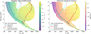 |
Fig. 1 (a) Spatial variations in magnetic Reynolds number (RM (Eq. (22)), left) and (b) thermal ionization fraction (xe, right) for WASP-18 b. Large areas of the dayside are in the intermediate and high-RM regimes, while ionization varies over many orders of magnitude, motivating an anisotropic drag treatment that accounts for local conductivity and magnetic geometry. The lines show gas temperature-pressure profiles averaged over all latitudes and over different regions in the atmosphere: dayside (−90◦< ϕ ≤ 90◦), nightside (|ϕ| > 90◦), morning (−97.5◦≤ ϕ ≤ −82.5◦) and evening terminator (82.5◦≥ ϕ ≥ 97.5◦). The results of the simulation with anisotropic drag were used in the calculation of RM, xe, and the averaged temperature-pressure profiles shown here. |
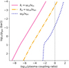 |
Fig. 2 Magnetization parameter (Eq. (21)) profiles for ions (ki) and electrons (ke) averaged over all latitudes and over dayside atmosphere (−90◦< ϕ ≤ 90◦). The dotted blue line (ωpe/νen) shows the relation between the electron plasma frequency and the electron–neutral collision frequency averaged over the dayside atmosphere. The plasma coupling ratios were calculated from the ExoRad simulation for WASP-18 b with anisotropic drag. The dashed gray line shows where the plasma coupling ratio reaches unity. |
4.1 Where does magnetic drag affect atmosphere environments?
The efficiency and geometry of the momentum exchange strongly depend on xe, the local magnetic field orientation, and the relative importance of inductive and diffusive processes. The existing active drag parameterization used in GCM studies of hot Jupiters (e.g., Rauscher & Menou 2013) scales with the local magnetic diffusivity, η (Eq. (A.21)). While this approach captures the braking of the wind flow on the dayside, it treats the drag as isotropic, only affecting the zonal component of the wind velocity but taking into account the variations in the ionization on the day- and nightside. This approach is valid only for RM ≪ 1 (e.g., Dietrich et al. 2022), where the plasma is only weakly coupled to the field, the magnetic diffusion dominates, and the field lines move freely through the gas. In this case the magnetic field only weakly affects the flow. However, this model does not take into account that the interaction between a conducting fluid and a magnetic field is anisotropic, which becomes important for the intermediate RM regime (RM ≈ 1). Charged particles are constrained to move along magnetic field lines, while their movement perpendicular to the field is restricted. This leads to an anisotropic drag force on the neutral gas. In Fig. 1a, a map of the Reynolds number for the modeled atmospheric structure shows that large regions of the dayside extend into the intermediate-to-high RM regime. Inductive effects become important where RM > 1 and drag is anisotropic, while the cooler nightside and deeper layers have RM ≪ 1. The anisotropic magnetic drag is represented by separating the Pedersen and Hall contributions, which are the dissipative and non-dissipative components of the magnetic drag, respectively. The Pedersen component corresponds to drag perpendicular to the magnetic field, leading to flow damping and kinetic energy loss, whereas the Hall component corresponds to drag perpendicular to both the magnetic field and the flow velocity, modifying the flow direction without energy dissipation. As the starting point, the momentum equations for ions, electrons, and neutrals were taken (Eqs. (24)–(26)). Then drift velocities of the charged particles with respect to the neutrals were derived (Eq. (31)) and were used to parametrize the magnetic drag force (Eq. (36)) acting on the neutral gas. This formulation of the anisotropic drag is applicable across low and intermediate RM regimes and is a significant physical improvement over isotropic drag models, providing a more realistic representation of the directional property of the Lorentz force in the large areas of the atmosphere where the low and intermediate RM approximation is valid. In the region where RM ≫ 1, the magnetic field lines are frozen into the plasma and advection dominates over diffusion. Here, the atmospheric gas and magnetic field are fully coupled: the gas and field move together, inducing strong currents and feedback reactions on the flow Rogers (2017). For this, a fully self-consistent MHD treatment would be required for accuracy. However, it should be noted that RM must be interpreted carefully in the presence of strong magnetic drag. Strong drag can suppress the horizontal flow, resulting in small values of RM that represent a reduced velocity rather than weak magnetic coupling. Therefore, a small RM does not necessarily demonstrate if a magnetic drag parametrization is valid in this regime, as the flow might be in the ideal MHD limit. To analyze the system properly, not only RM but the plasma parameters introduced before need to be considered (Eqs. (19)–(23)).
4.2 Momentum exchange between charged and neutral species and frictional heating
The following derivations are described in a right-handed spherical coordinate system defined by the radial distance, r [m], latitude, θ [◦], and longitude, ϕ [◦], with the corresponding unit vectors,  (radially outward),
  (positive northward), and
  (positive eastward). This coordinate system, which is in height coordinates, differs from the p coordinates in which the HPEs (Eqs. (1)–(4)) are solved primarily because the vertical coordinate itself changes the meaning of vertical derivatives and the different surfaces (gas pressure vs. geometric height) on which the horizontal gradients of fields are defined.
In the planet’s rotating reference frame, the momentum equation for the neutral species is given by (see Song et al. 2001)
 (24)
(24)
where  is the velocity vector of the neutral species with the radial velocity, vn,r [m s−1], the zonal velocity, vn,ϕ [m s−1], and the meridional velocity, vn,θ [m s−1], pgas [Pa] the gas pressure of the neutral species, Fn the sum of external forces acting on the neutrals (e.g., gravity, Coriolis, centrifugal), ρi [kg m−3] the ion mass density, ρe [kg m−3] the electron mass density, and ρn [kg m−3] the neutral mass density, and νin, νen [s−1] the ion-neutral and electron-neutral collision frequencies, respectively. The last two terms on the right-hand side represent the frictional drag resulting from the relative motion between charged and neutral species. In this paper, only gas species are considered. The momentum Eq. (24) without the frictional terms in height coordinates is equivalent to the horizontal and vertical momentum (Eqs. (1) and (2)) in p coordinates using the hydrostatic balance assumption in the vertical direction.
The momentum equations for electrons (subscript s = e) and ions (s = i) are given by (see, e.g., Song et al. 2001)
 (25)
(25)
 (26)
(26)
where e [C] is the elementary charge, Fs the external forces exerting on the charged species, s, and ns [m−3], Ps [Pa], and ms [kg] the number density, pressure, and mass of each charged species, respectively. E and B are the electric and magnetic fields. Here, the terms with electron-ion collision frequency, νei, and ion-electron collision frequency, νie, were neglected, since our estimates have shown that for our parameter regime νen ≫ νei and νin ≫ νie. Since ExoRad does not evolve ion or electron dynamics, a steady-state approximation  for their drift velocities was derived using a reduced momentum balance equation for electrons and ions, assuming singly charged ions, quasi-neutrality, and neglecting pressure gradients and inertial terms (e.g., Schunk & Nagy 2009):
 (27)
(27)
We further assumed that the large-scale electric field in the planetary rest frame is negligible (E ≈ 0). This implies that the electric field in the local frame of the neutral fluid is E′ = E+ vn × B ≈ vn× B. This approach does not take into account the feedback from the global current system, which would modify the large scale electric field and currents. The main limitation of the model is that it neglects the polarization electric field and therefore does not ensure current closure. In a partially ionized atmosphere, collisions between neutrals and charged particles introduce charge separation, which creates a polarization electric field. This field is built up until it balances the differential drifts of ions and electrons, though it maintains current continuity by diverting currents within the ionosphere. By neglecting the polarization field, the model only describes the local Lorentz force component of the coupling between charged particles and neutrals, without taking into account any self-consistent electrodynamic feedback in the ionosphere. Therefore, the calculated magnetic drag describes a local forcing approximation rather than the global response of an ionospheric current system. However, this parametrization provides a physically based and computationally efficient method of studying the main large-scale effects of magnetic coupling on the atmospheric dynamics and thermal structure. The model separates the impact of direct collisional drag between charged particles and neutrals, which dominates in the upper atmosphere. Nevertheless, a more complete approach, i.e., solving the Poisson’s equation, would enable global current closure and feedback from large-scale electric fields (see Sect. 6). These effects could modify the magnitude and spatial distribution of the frictional drag and heating. This, however, is outside the scope of the present paper.
We further assumed a dipolar large-scale planetary magnetic field anti-aligned with the planetary rotation axis. The field is purely poloidal, with the magnetic flux density given by
 (28)
(28)
To calculate the dipolar magnetic field, the equatorial magnetic field strength, B0 [T], was defined at the reference radius, Rref [m] (Sect. 2). The northward component, Bdip,θ [T], is positive in the direction of increasing θ. The magnitude of the magnetic field, |Bdip|, and its unit vector,  , are
, are
 (29)
(29)
 (30)
(30)
To simplify the implementation, the r dependence of the magnetic field is neglected in the simulations of ExoRad. Treating Bdip as constant with altitude introduces only a small error of less than 4% in |Bdip| in the modeled atmospheric region of WASP-18 b, corresponding to a radial extent of ∆z ≈ 1075 km. This estimate is specific to the geometry and scale height of WASP-18 b. In (U)HJs with more extended atmospheres or smaller radii, the variation in Bdip with altitude could be more pronounced and should be accounted for in the analysis. Additionally, it is assumed for the drag calculation that the neutral wind has no radial component (vn,r ≈ 0 m/s), as vertical winds are weak compared to horizontal winds. Solving Eq. (27) for the drift velocity Δvs = vs −vn yields
 (31)
(31)
where the upper sign applies to ions (s = i) and the lower one to electrons (s = e). The velocity of the neutrals perpendicular to Bdip is given by
 (32)
(32)
Equation (31) shows that if ks ≪ 1, collisions dominate and the charged species are strongly coupled to the neutrals. In this regime, magnetic drag is weak. For ks ≫ 1, the charged particles complete many gyro-orbits before being deflected by collisions. They are magnetized and coupled primarily to the magnetic field, leading to significant relative drift and enhanced magnetic drag on the neutrals. Substituting Eq. (31) into the momentum exchange terms of Eq. (24), the total drag force density exerted by charged particles on the neutral fluid is
 (33)
(33)
To estimate the contributions from ion and electron drag, the Pedersen KP,s [kg m−3s−1] and Hall drag coefficients, KH,s [kg m−3s−1], for each species are introduced:
 (34)
(34)
 (35)
(35)
so that the total drag force density simplifies to
 (36)
(36)
The first term represents the Hall drag, which acts perpendicular to both vn and Bdip, while the second term corresponds to the Pedersen drag, which opposes the perpendicular motion of the neutrals to Bdip. Although ion and electron velocities are not evolved dynamically, their influence is included through the Hall and Pedersen coefficients, which depend on local xe, plasma parameters, and magnetic field strength of the dipolar field. With Eq. (23) the electron and ion mass density (ρs = msxenn) can be calculated.
ExoRad assumes vertical hydrostatic equilibrium, employing gas pressure as the vertical coordinate. It does not explicitly solve the vertical momentum equation. Instead, vertical velocities are derived to ensure mass continuity. While vertical magnetic drag forces can occur (e.g., Christie et al. 2025), their inclusion would violate the vertical hydrostatic equilibrium. However, the resulting vertical acceleration is expected to be negligibly small compared to gravity in the weakly ionized regime considered here. Therefore, the radial drag is neglected and only the meridional and zonal components of the drag force density are computed:
 (37)
(37)
 (38)
(38)
where
![Mathematical equation: ${K_H} = {K_{H,i}} - {K_{H,e}}\left[ {{\rm{kg}}{{\rm{m}}^{ - 3}}{{\rm{s}}^{ - 1}}} \right],$](/articles/aa/full_html/2026/04/aa58210-25/aa58210-25-eq63.png) (39)
(39)
![Mathematical equation: ${K_P} = {K_{P,e}} + {K_{P,i}}\left[ {{\rm{kg}}{{\rm{m}}^{ - 3}}{{\rm{s}}^{ - 1}}} \right],$](/articles/aa/full_html/2026/04/aa58210-25/aa58210-25-eq64.png) (40)
(40)
are the total Hall and Pedersen coefficients, respectively. The geometric relation  was used, assuming the azimuthal component of the magnetic field to be negligible
  . The expression in Eqs. (37) and (38) was implemented in ExoRad as an external drag force acting on the horizontal momentum Eq. (1) via
  and νen are
 (41)
(41)
 (42)
(42)
where nn [m−3] is the neutral number density. The electron-H collision rate follows Koskinen et al. (2010), based on Danby et al. (1996). The chemical atmosphere gas composition strongly varies between the day- and nightside. While the dayside is dominated by atomic H, the nightside is dominated by H2 (Fig. 8 of Helling et al. 2019a). In this work, νen was computed assuming atomic hydrogen as the dominant neutral species, which is justified on the dayside of WASP-18 b. On the nightside, where molecular hydrogen dominates, νen might be underestimated, as collision frequencies differ (Eq. (12) in Koskinen et al. 2010). However, the electron density and therefore the magnetic coupling strongly decrease on the nightside and the resulting impact on the magnetic drag is small. The ion-neutral rate is based on a rigid-sphere model for non-resonant collisions (Chapman 1956; Günzkofer et al. 2023), assuming a mean atomic mass number of 32 that was estimated by summing the relevant atomic masses that make up an ion as given in GGchem. However, the effective ion mass may vary with altitude and longitude as the dominant ion species is determined by the gas temperature and elemental abundances. In the plasma regime considered here, ions are collisionally coupled to the neutrals (ki ≪ 1; Fig. 2), so the resulting variations in ion mass have a comparatively weak effect on the conductivities relative to the dominant dependence on electron density. Therefore, the assumed constant mass number is sufficient for the present work; however, future studies including altitude-dependent ion composition would be valuable. Resonant collisions (e.g., Na+–Na) are negligible due to the dominance of hydrogen in the neutral atmosphere.
The total drag force density (Eq. (36)) provides both a sink of momentum and a source of frictional heating, and is particularly important where the magnetization parameters, ki and ke, are large. In Fig. 3, the Hall and Pedersen drag coefficients according to Eqs. (34) and (35) were calculated using the gas pressure (pgas) and temperature (Tgas) output from the ExoRad simulation of the WASP-18 b atmosphere with anisotropic magnetic drag, as well as xe output from GGchem. The coefficients shown are averaged over all latitudes and over the dayside atmosphere (−90◦< ϕ ≤ 90◦). For pgas ≥ 10−3 bar, KH,e and KH,i (orange lines) are of similar magnitude and largely cancel out due to opposite signs (KH, magenta line), making the electron Pedersen drag (KP,e, dotted cyan line) the dominant contributor. At higher altitudes where pgas < 10−3 bar, ke > 1 and ki < 1 (see Fig. 2) but the small electron mass suppresses KH,e, so KH,i dominates the total Hall drag (KH) and the Hall drag dominates the total Pedersen drag (KP). To maintain the numerical stability in ExoRad (Sect. 2), the drag timescale is constrained to τdrag = min(ρn/KH, ρn/KP) ≥ 100 s. Consequently, the imposed lower limit reduces the effective drag strength at low pressures. Therefore, the dayside-averaged KP deviates from its physically expected value at pgas < 10−2 bar (gray line in Fig. 3), and KH at pgas ≲ 10−3 bar.
In addition to affecting neutral momentum, magnetic drag contributes to energy dissipation via frictional heating. The heating of the neutral atmosphere due to magnetic drag is often referred to as Joule or Ohmic heating, but it is more accurately described as frictional heating resulting from momentum exchange between drifting charged particles and neutrals and not electromagnetic dissipation, which results from electric currents interacting with the electrical resistivity of the gas (Vasyliūnas & Song 2005). For energy to be conserved, the corresponding rate at which energy is dissipated into heat per unit mass of the neutral gas is equal to the rate at which Pedersen drag force works on the fluid, given by
 (43)
(43)
qfric is always positive, as it represents a conversion of neutral kinetic energy into thermal energy. The Hall drag force is a deflective force: it changes the direction of the flow but does not remove kinetic energy from the flow. The Pedersen drag component is frictional and removes kinetic energy from the flow, which is converted into heat. To include the frictional heating in the energy equation in ExoRad, qfric is evaluated at each time step and added to the potential temperature tendency equation.
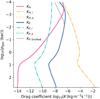 |
Fig. 3 Hall (KH,s) and Pedersen (KP,s) drag coefficients for electrons (s = e) and ions (s = i) averaged over all latitudes and over dayside atmosphere (−90◦< ϕ ≤ 90◦). KH = KH,i − KH,e and KP = KP,i + KP,e are the total Hall and Pedersen coefficients. The coefficients were calculated using the gas pressure-temperature profile from the ExoRad simulation run of WASP-18 b with anisotropic drag. The gray line shows KP obtained directly from ExoRad. It diverges from the calculated KP (blue line) in the upper atmosphere because the drag timescale in ExoRad is limited to τdrag ≥ 100 s. The same applies for KH from ExoRad (not shown here). |
5 Impact of magnetic drag on winds and temperatures in the atmosphere of WASP-18 b
Magnetic drag is expected to be crucial in shaping UHJs atmospheres, yet its effects remain insufficiently studied and constrained. Here, it is shown how magnetic drag modifies the wind pattern and thermal structure in the atmosphere of WASP-18 b and how different magnetic drag models compare to each other. The extent to which the magnetic drag disrupts the equatorial super-rotation, how it modifies heat redistribution between day and night, and whether it can change the flow pattern will be explored. The results show that magnetic drag generally weakens equatorial super-rotation, and that anisotropic drag can lead to a flow decoupling and deflection between the day- and nightside.
5.1 Atmospheric circulation and different drag treatments
Figure 4 shows the horizontal wind speeds and streamlines for the different drag treatments (no drag, uniform drag, active drag, and anisotropic drag) for WASP-18 b as a test case planet. Figure 5 shows the corresponding mean zonal wind structures. In the absence of magnetic drag (when momentum and energy transfers are unaffected by the magnetic drag), the circulation is dominated by a pronounced eastward (super-rotating) equatorial jet extending across the planet. However, the strength of the jet is weakened in the upper dayside atmosphere (pgas ≤ 10−3 bar: Figs. 4a, 5a), likely as a result of radiative cooling and heating or vertical wind shear. The upper atmosphere is more strongly affected by direct stellar irradiation and less by advection compared to the denser lower atmosphere. The strong irradiation then heats the lower atmosphere and determines the thermal structure via radiative processes. Steep thermal gradients from irradiation create vertical wind shear of the zonal wind. Such shear leads to momentum redistribution and weakening of the zonal jet in the upper atmosphere. Thus, radiative processes play an important role in the upper atmosphere, while advective heat redistribution is more dominant in the lower atmosphere. This circulation pattern is common in hot Jupiter simulations without magnetic drag (e.g., Showman et al. 2009; Showman & Polvani 2010, 2011), driven by a Matsuno–Gill–type response (Matsuno 1966; Gill 1980). Peak horizontal wind speeds exceed 10 km/s.
If a constant magnetic drag acts uniformly on the horizontal momentum and energy transfer (uniform drag), the equatorial super-rotating jet is largely suppressed (Figs. 4b, 4f, and 5j). The circulation is instead dominated by eastward and westward flows of comparable magnitude, which mostly cancel in the zonal mean (Fig. 5j). Similar to Beltz et al. (2022b, see their Fig. 8 for the total atmosphere), a weaker eastward jet is present at pgas < 1 bar in higher latitudes (|ϕ| > 50◦) on the day-side atmosphere (Fig. 5b). On the nightside (Fig. 5f), a weak and narrow equatorial jet is visible for pgas < 10−3 bar. The circulation is concentrated near the day–night terminators (longitudes ≈ ± 90◦), with enhanced horizontal wind speeds. The flow diverges out of the substellar region. Uniform drag removes momentum throughout the atmosphere uniformly, damping the wave–driven feedback that sustains the equatorial super-rotation. Hence, a strong global uniform drag damps the equatorial jet throughout the entire atmosphere. However, such a model does not capture the underlying physics, since it neglects the strong spatial variability of the ionization fraction, particularly on the day- and nightside, resulting in magnetic coupling of both the dayside and nightside.
A drag confined only to the zonal direction (active drag; Figs. 4c and 4g) opposes the zonal flow and decouples the day-to nightside flow completely (at pgas < 10−3 bar), and therefore suppresses the equatorial jet on the dayside (Fig. 5c). At low pressures higher in the atmosphere, where drag timescales are extremely short, the zonal (east–west) flow is efficiently damped and the flow on the dayside is redirected toward the poles, producing a largely meridional (north–south) circulation on the dayside (Figs. 4c and 5c), consistent with previous studies (e.g., Beltz et al. 2022b). A zonal magnetic drag is based on the assumption that only meridional currents affect the atmospheric dynamics. The vanishing of the zonal magnetic drag at the equator due to the sin θ dependence in Eqs. (A.14) and (A.15) has previously been discussed by Christie et al. (2025) and is visible in the streamline in the zonal direction at θ = 0◦ on the dayside in the upper atmosphere (Fig. 4c. At higher pressures (pgas = 10−1 bar; Fig. 4g), where drag is weaker, zonal flow partially recovers, but meridional flow remains the dominant component.
A more complete representation of the effect of a planetary dipole magnetic field is achieved with a magnetic drag force acting in both the zonal and meridional directions (anisotropic drag). The drag strongly damps the flow, especially at low gas pressures (pgas = 10−3 bar) on the dayside (Figs. 4d and 5d).
The resulting magnetic drag forces effectively isolate the day-side from the nightside circulation at the equatorial region at the morning terminator (ϕ ≈ −90◦; Fig. 4d). At higher latitudes (ϕ > |30◦|) at the morning terminator, the gas flow is restored from the dayside to the nightside. At the evening terminator (ϕ ≈ 90◦), the streamlines are directed from the dayside to the nightside. Despite this strong damping, an eastward equatorial jet remains on the nightside and extends over a broader latitude range than in the active drag case (Fig. 5h). The wind speed shows dayside stagnation with limited redistribution, coupled to a nightside jet sustained by momentum convergence from deeper levels. This indicates that anisotropic drag firstly acts to dissipate kinetic energy, slow down, and deflect the flow on the dayside, while still allowing the equatorial jet to be maintained on the nightside. The Pedersen drag primarily suppresses zonal winds, producing significantly reduced flow speeds on the dayside, and the Hall drag generates a non-dissipative magnetic coupling between the meridional and zonal flow components (Eqs. (37) and (38)). In the upper atmosphere, where the Hall drag strength becomes comparable to the Pedersen drag, the Hall drag introduces an asymmetry in the flow pattern. This asymmetry is visible in Fig. 4d in the dayside streamlines between −90◦ < ϕ < 0◦ and 0◦ < ϕ < 90◦. In the longitude range −90◦ < ϕ < 0◦, the Hall drag deflects the flow toward more polar-directed motion, whereas in 0◦ < ϕ < 90◦ the stream lines show increased curvature and are redirected toward the evening terminator. If the magnetic dipole is aligned with the planetary rotation axis (not shown here),  (Eq. (30)) changes sign while maintaining the same magnitude. In that case, the Pedersen damping does not change, but the magnetic coupling produced by the Hall drag between vn,θ and vn,ϕ reverses sign, leading to a circulation pattern, which is mirrored on the day-side with enhanced curvature occurring in −90◦ < ϕ < 0◦ and more meridional flow in 0◦ < ϕ < 90◦. This behavior demonstrates the strong dependence of the atmospheric flow on the magnetic field geometry in the upper atmosphere. The resulting flow asymmetry determines the distribution of momentum across the terminator regions and indirectly affects the flow on the nightside. The flow perturbations due to the Hall effect on the nightside do not arise from strong local Hall drag, which is weak due to low ionization fraction, but are instead a nonlocal response from the redirected momentum on the dayside. At the poles on the dayside where the magnetic field lines are nearly vertical, the flow experiences a stronger drag in the meridional direction than at the equator where the field lines are horizontal, meridional magnetic drag force vanishes, and only the zonal velocity is damped by the Pedersen drag component. This is seen in Eqs. (37) and (38), where the polar flow structure is produced by the dominance of the radial magnetic field component, which reaches
  at the poles. Both Pedersen (in the meridional direction of the magnetic drag force) and Hall drag terms are increased in the polar regions. The Pedersen drag provides strong damping, particularly in the meridional direction, where the damping scales as
  , producing strong suppression of polar motions. On the other hand, the Hall drag couples the zonal and meridional velocity components through terms proportional to
  , creating a rotation of the horizontal momentum. The Hall term rotates the velocity vector against strong Pedersen damping, producing the flow curvature and directional asymmetry seen in the polar regions (Fig. 4d). At gas pressures of 1 mbar, the overall wind structure is similar to that shown by Christie et al. (2025, their Fig. 13). However, unlike in the results shown here, the wind flow in Christie et al. (2025) for their anisotropic approach does not experience longitudinal asymmetries due to the Hall drag and the partial decoupling of the equatorial jet at the morning terminator. The hottest planet considered in Christie et al. (2025) reaches lower dayside temperatures than WASP-18 b, resulting in a negligible contribution of the Hall term in the drag force.
In both the active drag and anisotropic drag cases, the equatorial jet reestablishes on the dayside for pgas > 10−2 bar (active drag, Fig. 5c) and pgas > 10−1 bar (anisotropic drag, Fig. 5d). While the variation in jet width with pressure is similar in the anisotropic drag and no drag cases (compare Figs. 5e and 5h), the jet in the active drag case is narrower. Plaschzug et al. (2026) introduced the width of the equatorial jet as well as the wind speed as two of four climate characteristics to help characterize the potential diversity of climate regimes in the ensemble of gas giant exoplanets (see their Fig. 5). Table 3 shows how jet width and wind speeds are affected by magnetic drag. The comparison between the parameters of a planet with an F host star and a global temperature of 2400 K from Fig. 5 of Plaschzug et al. (2026) and the calculated parameters from this study for the case in which magnetic effects are absent (no drag; Table 3) shows that the wind jet width is significantly larger, the evening-morning temperature difference is smaller, and the day-nightside temperature difference is larger in this study. This discrepancy might come from different initial conditions for the planet and the exclusion of TiO and VO in the simulations for UHJs in Plaschzug et al. (2026). Including TiO and VO leads to upper dayside atmosphere thermal inversion, as is seen for example in the red line of Fig. 1. Deline et al. (2025) have shown that including magnetic drag and the strong local gas-phase absorber TiO and VO are important to fit the data from optical to IR wavelengths for WASP-18 b. The wind velocity is the highest when the magnetic drag is absent and lowest when the drag force acts uniformly on the horizontal flow, implying that the magnetic drag significantly reduces the maximum wind speeds.
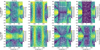 |
Fig. 4 Maps of horizontal wind speed |vh| and streamlines (white lines) at two pressure levels (pgas =0.1 bar and pgas =0.001 bar) for the four different magnetic drag treatments (no drag, uniform drag, active drag, and anisotropic drag). The substellar point is centered at each map. The vertical dashed black lines mark the area at longitude ±90◦. The output of each velocity component is time-averaged over 100 days of simulation time to eliminate the small-scale fluctuations. |
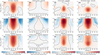 |
Fig. 5 Mean zonal wind for the four different magnetic drag treatments in different regions of the atmosphere: dayside atmosphere (first row), nightside atmosphere (second row), and total atmosphere (third row). The zonal wind velocity, u, is averaged at a specific latitude, and pressure level across longitudes on the dayside (−90◦≤ ϕ ≤ 90◦), on the nightside (|ϕ| > 90◦), and all longitudes. The black line shows the zero-wind contour, the boundary between super-rotation and counter-rotation. The output of the zonal wind velocity is time-averaged over 100 days of simulation time to eliminate the small-scale fluctuations. |
5.2 Gas temperature and different drag treatments
In Fig. 6, horizontal temperature maps for different drag treatments and pressure levels and the hotspot regions are shown. When active drag, anisotropic drag, or no drag is applied to the atmospheric flow, a hotspot splitting in the upper atmosphere (pgas = 10−3 bar) is observed almost symmetric around the equator where two distinct temperature maxima regions instead of one appear. This kind of splitting was also seen in other models (e.g., Carone et al. 2020; Komacek & Showman 2016). In Fig. 6e, a strong eastward equatorial jet is visible (see white arrows), which transports heat efficiently from the substellar point eastward, resulting in an eastward shift of the peak temperature (see cyan contours). The wind direction around the equator is almost purely zonal. When this wind flow slightly changes so that wind also points in the meridional direction, these winds shear the hottest region apart and redistribute it meridionally (Fig. 6a). The hotspots can be seen then as two symmetric lobes around the equator. If magnetic drag acts uniformly in the atmosphere, the hotspot area is almost centered at the substellar point because the equatorial jet is suppressed (Figs. 6b and 6f). Here, the momentum damping is constant.
The active and anisotropic drag introduce a nonlinear feedback that arises because neutral winds adjust the induced electric field  , which drives currents. These currents depend on the locally varying conductivities. Then they act back on the winds via damping and Hall deflection (only in the anisotropic drag case). Therefore, these cases suppress equatorial super-rotation on the dayside at low pressures (Figs. 5c, d) and distort zonal flows, leading to no efficient eastward advection of heat. When strong magnetic drag (Pedersen + Hall) acts on the flow, it damps the wave response. The circulation then becomes less wave-driven and more controlled by pressure-gradient forces. In Table 3 the location of the maximum temperatures for the different drag treatments at pgas = 10−1 bar is summarized. In the case of active and anisotropic drag, a shift of Tmax eastward of the substellar point by 7.5◦ is seen, which is less compared to the case in which no magnetic drag is applied to the atmosphere (12.5◦). The reason is that the magnetic drag suppresses or reduces the eastward equatorial jet. This was also proposed by previous studies; for example, Rogers & Komacek (2014) and Kataria et al. (2015). In the active drag and anisotropic drag cases, an asymmetry of the hotspot regions emerges (Figs. 6c, 6d, 6g, 6h). In the active drag model, the primary hotspot region is displaced by ∼20◦ south of the equator. A secondary hotspot region develops ∼20◦ north of the equator, but its temperature remains about 10 K cooler than the southern hotspot at pgas = 10−1 bar. Hence, locally changing drag forces and energy inputs may introduce another level of observable asymmetries; namely, in the form of a primary and a secondary hotspot region. Furthermore, the transition region between the cooler nightside and hot dayside at the morning terminator is shifted eastward at pgas = 10−1 bar around the equatorial region for the no drag, active drag, and anisotropic drag cases, with the shift in the no drag being the strongest and the one in the anisotropic drag being the weakest (compare the transition region to the position of the dashed black line at ϕ = −90◦ in Figs. 6e, 6g, and 6h). A similar eastward shift is observed at the evening terminator. This eastward shift of the day–night boundary appears due to the zonal advection of heat by the equatorial jet, which transports the thermal hotspot downstream of the substellar point. When magnetic drag is introduced, Lorentz forces act against the zonal flow and dissipate kinetic energy, thereby weakening the jet and reducing the longitudinal offset of the thermal transition region. Consequently, stronger or more spatially extended drag (anisotropic drag) suppresses the eastward shift of the terminator.
Figure 7 shows the gas temperature-pressure profiles averaged across all latitudes within different longitude regions for the four drag treatments. All models show a strong difference between the day- and nightside in the upper atmosphere, with the dayside reaching almost 3000 K and the nightside remaining below 1100 K. The profiles of the terminator regions lie in between, with the evening terminator being warmer than the morning terminator for the no drag, active drag, and anisotropic drag models, consistent with the eastward-directed flow that advects hot material. When a spatially uniform magnetic drag is applied, the terminator profiles almost overlap for pgas < 10−1 bar. The temperature differences between the day- and night-side and between the evening and morning terminator, the two remaining climate characteristics (Plaschzug et al. 2026), are displayed in Table 3. It shows that the difference between the averaged temperatures on the morning and evening terminator at pgas = 10−1 bar is strongest in the anisotropic drag case, with the evening terminator being 20% hotter than the morning terminator, and weakest in the uniform drag treatment. Temperature inversions are present on the dayside and absent on the nightside. On the nightside, the magnetic drag also affects the temperature profiles. The temperatures are lower when magnetic drag is acting on the atmospheric dynamics (active drag and anisotropic drag) compared to the case in which magnetic field does not affect the dynamics (no drag). The nightside temperature of the uniform drag model is larger than for the other cases and almost constant for pgas < 10−1 bar, which is due to the suppression of zonal heat redistribution. In the uniform drag case, the temperature inversion at the dayside is stronger and lies deeper in the atmosphere (pgas = 10 bar) than for the other drag treatments. This is also the case for the evening and morning terminator regions. At pgas > 10 bar, the profiles converge across the regions for all drag treatments, indicating that the deeper atmosphere is much less affected by the drag.
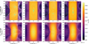 |
Fig. 6 Maps of gas temperature and velocity field at two gas pressure levels (pgas = 0.1 bar and pgas = 0.001 bar) for the four different magnetic drag treatments. The substellar point is centered at each map and is marked with a white star. The velocity field is shown by the white arrows. The length of the arrow scales with the relative wind velocity. The vertical dashed black lines mark the area at longitude ±90◦. The cyan contours represent the hotspot region (Tgas,max, Tgas,max − 1K) with Tgas,max being the largest temperature for the chosen pressure level. The temperature is time-averaged over 100 days of simulation time to eliminate the small-scale fluctuations. |
ExoRad results: Effect of magnetic drag on WASP-18 b’s climate state characteristics.
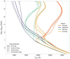 |
Fig. 7 Gas temperature-pressure profiles for four different drag treatments averaged over all latitudes and over different regions in the atmosphere: dayside (−90◦< ϕ ≤ 90◦), nightside (|ϕ| > 90◦), morning terminator (−97.5◦≤ ϕ ≤ −82.5◦), and evening terminator (82.5◦≥ ϕ ≥ 97.5◦). All drag treatments show pronounced day-night differences and temperature inversions in the upper atmosphere. Nightside temperatures are cooler when active or anisotropic magnetic drag is applied compared to no drag. |
6 Discussion
The implementation of the anisotropic magnetic drag demonstrates that magnetic effects can significantly reshape the atmospheric circulation of UHJs. The main outcome is that the magnetic drag disrupts the equatorial super-rotation on the day-side, thereby decoupling the dayside and nightside circulations at the equatorial region in the upper atmosphere, deflecting the flow on the dayside, and altering the efficiency of heat redistribution. The drag dissipates kinetic energy and dampens the flow, while maintaining an eastward jet of similar width on the nightside compared to an atmosphere that is not affected by the magnetic drag. Additionally, the dayside–nightside temperature difference increases and the hotspot and terminator shift toward the east becomes weaker. The implementation of anisotropic magnetic drag demonstrates an important step toward including plasma-neutral interactions in ExoRad, but several model limitations affect the interpretation of the simulation results.
Large-scale planetary electric field. A main simplification in the present model is the assumption of a negligible large-scale planetary electric potential  in the planetary rest frame. In reality, both dynamo-generated and polarization electric fields can arise from charge separation and currents. These fields influence the charged particle velocities, and hence the collisional drag felt by neutrals. By enforcing
  , the charged particle’s motion is controlled by
  . This includes the direct collisional drag but excludes feedback from electric fields. A self-consistent approach of the electric field would require one to solve a complex elliptic equation (Poisson’s equation) for the global polarization electric field across the atmosphere at every time step (e.g., Koskinen et al. 2014). Therefore, the current continuity equation (
 with the current density,
  , the conductivity tensor,
  , and the electric field seen in the frame of the neutrals,
  has to be solved and the equation to be calculated then becomes
  , where
  , which is electrostatic, is expressed as a gradient of a scalar potential
  . To solve the Poisson equation is computationally expensive and beyond the scope of the present work.
To make a rough estimate of the error that is made by neglecting  , Ohm’s law was considered:
  , where σP is the Pedersen (Eq. (B.2)), σH is the Hall (Eq. (B.3)), and σ∥ is the parallel conductivity (Eq. (A.23)), and the different components of the electric field are parallel
  and perpendicular
  to the magnetic field.
  arises from charge separation. The initial motional electric field,
  , drives two primary currents (Pedersen:
  , Hall:
  and causes charges to build up at the insulating boundaries (non-conducting nightside at terminator region, non-conducting gas above and below the ionosphere). The charge build-up creates
  opposing the initial charge flow. This means that
  drives a secondary Pedersen current
  that cancels out the primary Hall current
  to ensure
  . A simplified calculation of the polarization electric field with approximately uniform conductivities would require one to calculate
  , which gives
  drives a secondary Hall current
  . These currents flow in the same direction as the initial Pedersen drag current. The total drag current is then
  . The concept described here is analogous to the Earth’s equatorial electojet current system (e.g., Baumjohann & Treumann 1996; Muralikrishna & Kulkarni 2006). In this very simplified calculation, it was shown that neglecting
  , the anisotropic drag model underestimates both the magnetic drag force
  and the frictional heating rate by a factor of
  is shown in Fig. 2. So if ke ≈ 1 for pgas < 10−3 bar on the dayside atmosphere, then the magnetic drag force and the frictional heating are underestimated by a factor of 2. The model with anisotropic drag includes the initial electric field allowing the calculation of the primary magnetic drag but it neglects the secondary fields to ensure current closure. Therefore, the model underestimates the magnetic drag and frictional heating in the upper dayside atmosphere.
Nonideal MHD effects. Other magnetic effects such as ambipolar diffusion have also been neglected. The nonideal MHD effects can modify  and lead to modifications of the local Joule heating. To evaluate their relative importance, which influences the evolution of the magnetic field, the prefactors of the low-frequency Ohm’s law in the neutral frame, which is derived from the momentum equations of the electrons, ions, and the neutrals, can be approximated by (Leake et al. 2014; Ballester et al. 2018; Khomenko et al. 2014; Forteza et al. 2007)
 (44)
(44)
where  is the electric field in the neutral rest frame and
  is the electric current density. The terms on the right-hand side correspond to Ohmic diffusion, Hall effect, ambipolar diffusion, Biermann battery, and pressure-gradient contributions. The diffusion coefficients, scaled to units of m2 s−1, are given by
 (45)
(45)
Here the assumptions ke ≫ ki, mi ≫ me, ne ≈ ni = n, with the plasma number density, n [m−3], and the plasma pressure, p = pi + pe ≈ 2pe [Pa], have been applied. Note that in the estimation shown here, there is no difference made between the magnetic dipole field and the induced field, so B = Bdip. Effective diffusivities were introduced for the battery and pressure-gradient terms to enable a comparison with the diffusive terms: ![Mathematical equation: $\eta _{pe}^{{\rm{eff }}} = {{{p_e}} \over {|B|ne}}\left[ {{{\rm{m}}^2}{{\rm{s}}^{ - 1}}} \right]$](/articles/aa/full_html/2026/04/aa58210-25/aa58210-25-eq111.png) ,
, ![Mathematical equation: $\eta _{G,1}^{eff} = {{2{p_e}} \over {{\rho _i}{v_{in}}}}\left[ {{{\rm{m}}^2}{{\rm{s}}^{ - 1}}} \right]$](/articles/aa/full_html/2026/04/aa58210-25/aa58210-25-eq112.png) , and
, and ![Mathematical equation: $\eta _{G,2}^{eff} = {{{p_n}} \over {{\rho _n}{v_{in}}}}\left[ {{{\rm{m}}^2}{{\rm{s}}^{ - 1}}} \right]$](/articles/aa/full_html/2026/04/aa58210-25/aa58210-25-eq113.png) . As is shown in Fig. 8, the Hall effect and Ohmic diffusion dominate in the upper dayside atmosphere (pgas < 10−3 bar), with the Hall diffusivity exceeding the Ohmic diffusivity at the upper atmosphere. The other effects remain several orders of magnitude smaller than the Hall effect and Ohmic diffusion in the region of interest. Ambipolar diffusion has only a minor influence in the WASP-18 b case with a magnetic field strength of 5 G but possibly becomes relevant at pgas < 10−4 bar compared to Ohmic diffusion and Hall effects due to the decreasing gas number density. Since ηA is dependent on |B|2, increasing the magnetic field strength would enhance the effect of the ambipolar diffusion and it could become of a similar magnitude to the Ohmic diffusion at, for example, pgas < 10−3 bar for |B| = 50 G. However, ambipolar diffusion is linked to the feedback of the other MHD effects as well as the configuration of the dipolar and induced magnetic fields, and therefore the effect of the ambipolar diffusion might be different. Savel et al. (2024) proposed a new method of constraining the planetary magnetic field by measuring the ambipolar velocity in the photosphere via comparing heavy ion velocity with the neutral gas velocity using high-resolution spectroscopy. Therefore, this ambipolar diffusion effect can be relevant for studying the potential spectroscopical detectability of the ion-neutral velocity in the photosphere (Soriano-Guerrero et al. 2025). However, the interpretation of the results of this method strongly relies on the underlying model of the drift velocity between ions and neutrals (Christie et al. 2025, Appendix C). Pressure-gradient terms are negligible for the conditions applied here.
. As is shown in Fig. 8, the Hall effect and Ohmic diffusion dominate in the upper dayside atmosphere (pgas < 10−3 bar), with the Hall diffusivity exceeding the Ohmic diffusivity at the upper atmosphere. The other effects remain several orders of magnitude smaller than the Hall effect and Ohmic diffusion in the region of interest. Ambipolar diffusion has only a minor influence in the WASP-18 b case with a magnetic field strength of 5 G but possibly becomes relevant at pgas < 10−4 bar compared to Ohmic diffusion and Hall effects due to the decreasing gas number density. Since ηA is dependent on |B|2, increasing the magnetic field strength would enhance the effect of the ambipolar diffusion and it could become of a similar magnitude to the Ohmic diffusion at, for example, pgas < 10−3 bar for |B| = 50 G. However, ambipolar diffusion is linked to the feedback of the other MHD effects as well as the configuration of the dipolar and induced magnetic fields, and therefore the effect of the ambipolar diffusion might be different. Savel et al. (2024) proposed a new method of constraining the planetary magnetic field by measuring the ambipolar velocity in the photosphere via comparing heavy ion velocity with the neutral gas velocity using high-resolution spectroscopy. Therefore, this ambipolar diffusion effect can be relevant for studying the potential spectroscopical detectability of the ion-neutral velocity in the photosphere (Soriano-Guerrero et al. 2025). However, the interpretation of the results of this method strongly relies on the underlying model of the drift velocity between ions and neutrals (Christie et al. 2025, Appendix C). Pressure-gradient terms are negligible for the conditions applied here.
Self-excited atmospheric dynamo. Another limitation of the drag parameterization is the neglect of the effect of the atmospheric dynamo. For RM ≫ 1 (Fig. 4), atmospheric flows can produce toroidal fields comparable in strength to the imposed dipole field (Rogers & Komacek 2014). Several possible scenarios for atmospheric magnetic induction were explored by Dietrich et al. (2022), indicating that both the strength and geometry of the Lorentz force could show large variation from a static dipole configuration. In the present simulations, RM exceeds unity at pgas < 2 bar and peaks near RM ≈ 70 at ∼0.3 bar, suggesting that MHD effects could be dynamically important in this region. An approximate representation of these effects could be added in the model by modifying the magnitude of the magnetic field by a first-order correction; for example,  , where ϵ (0 < ϵ ≤ 1) is a parametrization that captures the enhancement of magnetic coupling when atmospheric induction becomes important. Here the balance between induction and diffusion was applied to estimate the induced magnetic field, Bind ∼ ϵRMBdip. ϵ can be calibrated by comparing the magnetic field profiles to MHD results (e.g., Rogers & Komacek 2014; Soriano-Guerrero et al. 2025).
Dipole magnetic field. The assumption of a dipolar planetary field remains reasonable as a first-order approximation for WASP-18 b. The morphology of the magnetic field depends on the balance between Coriolis and inertial forces in the convecting interior, characterized by the Rossby number  (Christensen & Aubert 2006). Taking characteristic values of U ∼ 0.1 m s−1 for the convective velocity, L ∼ 5 × 10⁷ m for the Jupiter-like shell thickness (Elias-López et al. 2025), and Ω = 7.7 × 10⁻⁵ rad s−1 for the angular velocity of WASP-18 b yields Ro ∼ 3 × 10⁻⁵. This value lies below the critical threshold of Ro ∼ 0.1, consistent with a dipole-dominated dynamo regime. Higher Rossby numbers (Ro > 0.1) indicate weaker, multipolar fields. However, U and L are uncertain and model-dependent, and the dynamo region of WASP-18 b is not directly constrained. Internal heating due to tides or Ohmic dissipation may affect the thickness and structure of the dynamo shell, which potentially favors a multipolar field (see, e.g., Stanley & Bloxham 2006). While the dipole assumption is reasonable for modeling atmospheric drag, the possibility of a multipolar magnetic field cannot be ruled out.
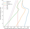 |
Fig. 8 Diffusion coefficients from the Ohm’s law (Eq. (6)) averaged over all latitudes and over dayside atmosphere (−90◦< ϕ ≤ 90◦). The coefficients were calculated from the output of the ExoRad simulation with anisotropic drag for the atmosphere of WASP-18 b. |
7 Summary
In this study, a physically motivated model for the anisotropic magnetic drag is presented to investigate how an anti-aligned planetary dipole magnetic field influences the atmospheric circulation of (U)HJs. This approach addresses the main research questions of (1) how magnetic coupling and the resulting drag modifies the wind circulation and hotspot shift, (2) to what extent the magnetic drag disrupts the equatorial super-rotation, and (3) how it alters heat distribution between the day- and nightside and the climate characteristics. By connecting the anisotropic drag approach to ionospheric conductivities and magnetization, the approach provides a theoretical framework for linking MHD processes to climate characteristics in UHJ atmospheres. Therefore, the magnetic drag parametrization was derived from a multi-fluid description in which electrons and ions are treated as magnetized species in steady-state momentum balance, collisionally coupled to the neutrals. The resulting ion and electron drift velocities relative to the neutrals were used to determine anisotropic drag in terms of Hall and Pedersen components acting on the neutral flow. The parametrization was implemented in the meridional and zonal momentum equations as well as in the temperature evolution equation of the cloud-free 3D GCM ExoRad, and applied to WASP-18 b. The results were compared with previously published drag treatments (uniform drag and active drag) and with simulations with an absent magnetic field influence. They demonstrate that the atmospheric circulation, in particular the presence and width of the equatorial super-rotating jet, strongly depend on the magnetic drag. The main findings are:
Anisotropic drag primarily dissipates kinetic energy and slows the flow on the dayside, while still allowing an efficient eastward equatorial jet to be maintained on the nightside, in contrast to uniform drag that suppresses overall wind flow. The presence or absence of anisotropic drag does not affect the width of the nightside jet but does affect the horizontal velocity of the jet;
Active drag completely decouples the dayside and night-side circulation in the upper atmosphere, leading to a slower nightside jet, a polar flow at the dayside, and a weaker eastward shift of the day–night boundary compared to the case in which the magnetic field is absent;
Anisotropic drag changes the dayside flow in particular for pgas ≤ 10−3 bar. The inclusion of the Hall term and the meridional drag component (Pedersen) leads to a deflection of the flow perpendicular to the dipole field. The result is a direct flow (albeit at a weaker level compared to uniform drag) from the dayside toward the nightside at the evening terminator at all latitudes and at the morning terminator at high latitudes (> |30◦|);
Identifying the wind flow direction over the terminators is thus important to identify the coupling regime (uniform: diverging flow from the substellar point, active: strong decoupling at terminator regions, anisotropic: only decoupled at equatorial morning terminator, otherwise dayside-to-nightside flow);
Because anisotropic drag includes more drag effects, this leads to an overall stronger damping of wind flow with smaller maximum velocities compared to the active drag;
With anisotropic drag the evening–morning terminator averaged temperature difference at pgas = 10−1 bar is stronger compared to the case without magnetic drag, with the evening terminator being 20% hotter than the morning terminator;
Both active and anisotropic drag reshape the circulation such that two hotspots appear north and south of the equator, with smaller eastward shifts compared to the case in which magnetic drag is absent. The results show that local variations in drag forces and energy can create observable asymmetries, producing both primary and secondary hotspot regions;
The morning-to-evening terminator gas temperature difference, ∆Tgas, at pgas = 10−3 bar (Table 3), is crucial to identify day-to-night side flow patterns arising with different drag treatments. Uniform drag with radial flow exhibits almost no contrast (∆Tgas ≈ 0 K), active drag with polar flow exhibits high contrast (∆Tgas = 145 K), and anisotropic drag due to partial horizontal flow toward the nightside exhibits lower contrast (∆Tgas ≈ 100 K).
While the parametrization of the magnetic drag includes the influence of Pedersen and Hall drag, it neglects several induction processes such as dynamo action, ambipolar diffusion, and ion and electron pressure effects. These processes likely become important in the partially ionized upper atmosphere, where RM ≳ 1, and may strongly determine both the efficiency and anisotropy of magnetic drag. Observationally, such uncertainties might impact predictions of phase curve amplitudes, hotspot offsets, transit asymmetries, and Doppler wind signatures. Because the model does not include the self-consistent evolution of the magnetic field, and thus neglects inductive feedback, it likely underestimates magnetic stresses. It is therefore not valid in atmospheric regions where RM ≫ 1. However, for RM ≲ 1, the parametrization provides reasonable estimates of the magnitude and direction of magnetic drag. Although the approach neglects the polarization electric field which arise to ensure global current closure, it remains a suitable and computationally efficient method of calculating the first-order effects of magnetic fields in a GCM. Understanding these effects and the extent to which they affect observations can provide a constraint on the magnetic field strengths of specific UHJs in future work.
Acknowledgements
A.B. thanks Maxim Khodachenko for useful discussions. The post-processing of GCM data has been performed with gcm-toolkit (Schneider et al. 2022b). The simulations (project id 72245) were performed on the Austrian Scientific Computing (ASC) infrastructure, in particular the Vienna Science Cluster (VSC). We thank the referee for very useful comments that improved this manuscript.
References
- Adcroft, A., Campin, J.-M., Hill, C., & Marshall, J. 2004, MWR, 132, 2845 [Google Scholar]
- Allard, N. F., Spiegelman, F., Leininger, T., & Molliere, P. 2019, A&A, 628, A120 [NASA ADS] [CrossRef] [EDP Sciences] [Google Scholar]
- Arakawa, A., & Lamb, V. R. 1977, in Methods in Computational Physics: Advances in Research and Applications, 17, General Circulation Models of the Atmosphere, ed. J. CHANG (Elsevier), 173 [Google Scholar]
- Arcangeli, J., Désert, J.-M., Parmentier, V., et al. 2019, A&A, 625, A136 [NASA ADS] [CrossRef] [EDP Sciences] [Google Scholar]
- Asplund, M., Grevesse, N., Sauval, A. J., & Scott, P. 2009, ARA&A, 47, 481 [NASA ADS] [CrossRef] [Google Scholar]
- Asplund, M., Amarsi, A. M., & Grevesse, N. 2021, A&A, 653, A141 [NASA ADS] [CrossRef] [EDP Sciences] [Google Scholar]
- Azzam, A. A. A., Tennyson, J., Yurchenko, S. N., & Naumenko, O. V. 2016, MNRAS, 460, 4063 [NASA ADS] [CrossRef] [Google Scholar]
- Baeyens, R., Désert, J.-M., Petrignani, A., Carone, L., & Schneider, A. D. 2024, A&A, 686, A24 [NASA ADS] [CrossRef] [EDP Sciences] [Google Scholar]
- Ballester, J. L., Alexeev, I., Collados, M., et al. 2018, Space Sci. Rev., 214, 58 [Google Scholar]
- Barber, R. J., Tennyson, J., Harris, G. J., & Tolchenov, R. N. 2006, MNRAS, 368, 1087 [Google Scholar]
- Barber, R. J., Strange, J. K., Hill, C., et al. 2014, MNRAS, 437, 1828 [CrossRef] [Google Scholar]
- Barton, E. J., Yurchenko, S. N., & Tennyson, J. 2013, MNRAS, 434, 1469 [NASA ADS] [CrossRef] [Google Scholar]
- Batygin, K., Stanley, S., & Stevenson, D. J. 2013, ApJ, 776, 53 [Google Scholar]
- Baumjohann, W., & Treumann, R. A. 1996, Basic Space Plasma physics Beltz, H., & Rauscher, E. 2024, ApJ, 976, 32 [Google Scholar]
- Beltz, H., Rauscher, E., Kempton, E. M.-R., et al. 2022a, AJ, 164, 140 [Google Scholar]
- Beltz, H., Rauscher, E., Roman, M. T., & Guilliat, A. 2022b, AJ, 163, 35 [Google Scholar]
- Beltz, H., Rauscher, E., Kempton, E. M.-R., Malsky, I., & Savel, A. B. 2023, AJ, 165, 257 [NASA ADS] [CrossRef] [Google Scholar]
- Beltz, H., Houck, W., Mayorga, L. C., et al. 2025, ApJ, 984, 90 [Google Scholar]
- Borysow, A. 2002, A&A, 390, 779 [NASA ADS] [CrossRef] [EDP Sciences] [Google Scholar]
- Borysow, A., & Frommhold, L. 1989, ApJ, 341, 549 [NASA ADS] [CrossRef] [Google Scholar]
- Borysow, J., Frommhold, L., & Birnbaum, G. 1988, ApJ, 326, 509 [NASA ADS] [CrossRef] [Google Scholar]
- Borysow, A., Frommhold, L., & Moraldi, M. 1989, ApJ, 336, 495 [NASA ADS] [CrossRef] [Google Scholar]
- Borysow, A., Jorgensen, U. G., & Fu, Y. 2001, J. Quant. Spec. Radiat. Transf., 68, 235 [NASA ADS] [CrossRef] [Google Scholar]
- Bougher, S. W., Waite, J. H., Majeed, T., & Gladstone, G. R. 2005, J. Geophys. Res.(Planets), 110, E04008 [Google Scholar]
- Burrows, A., Hubeny, I., Budaj, J., & Hubbard, W. B. 2007, ApJ, 661, 502 [NASA ADS] [CrossRef] [Google Scholar]
- Carone, L., Baeyens, R., Mollière, P., et al. 2020, MNRAS, 496, 3582 [NASA ADS] [CrossRef] [Google Scholar]
- Cauley, P. W., Shkolnik, E. L., Llama, J., & Lanza, A. F. 2019, Nat. Astron., 3, 1128 [NASA ADS] [CrossRef] [Google Scholar]
- Chan, Y. M., & Dalgarno, A. 1965, Proc. Phys. Soc., 85, 227 [NASA ADS] [CrossRef] [Google Scholar]
- Chapman, S. 1956, Il Nuovo Cimento, 4, 1385 [Google Scholar]
- Christensen, U. R., & Aubert, J. 2006, Geophys. J. Int., 166, 97 [NASA ADS] [CrossRef] [Google Scholar]
- Christensen, U. R., Holzwarth, V., & Reiners, A. 2009, Nature, 457, 167 [Google Scholar]
- Christie, D. A., Evans-Soma, T. M., Mayne, N. J., & Kohary, K. 2025, MNRAS, 541, 2773 [Google Scholar]
- Coles, P. A., Yurchenko, S. N., & Tennyson, J. 2019, MNRAS, 490, 4638 [CrossRef] [Google Scholar]
- Coulombe, L.-P., Benneke, B., Challener, R., et al. 2023, Nature, 620, 292 [NASA ADS] [CrossRef] [Google Scholar]
- Dalgarno, A., & Williams, D. A. 1962, ApJ, 136, 690 [NASA ADS] [CrossRef] [Google Scholar]
- Danby, G., Elza, B. K., Morrison, M. A., & Trail, W. K. 1996, J. Phys. B At. Mol. Phys., 29, 2265 [Google Scholar]
- Deline, A., Cubillos, P. E., Carone, L., et al. 2025, A&A, 699, A150 [NASA ADS] [CrossRef] [EDP Sciences] [Google Scholar]
- Dietrich, W., Kumar, S., Poser, A. J., et al. 2022, MNRAS, 517, 3113 [NASA ADS] [CrossRef] [Google Scholar]
- Draine, B. T., Roberge, W. G., & Dalgarno, A. 1983, ApJ, 264, 485 [CrossRef] [Google Scholar]
- Drummond, B., Mayne, N. J., Baraffe, I., et al. 2018, A&A, 612, A105 [NASA ADS] [CrossRef] [EDP Sciences] [Google Scholar]
- Edwards, J. M. 1996, J. Atmos. Sci., 53, 1921 [Google Scholar]
- Elias-López, A., Cantiello, M., Viganò, D., et al. 2025, ApJ, 990, 38 [Google Scholar]
- Feautrier, P. 1964, Comptes Rend. Acad. Sci.(serie non specifiee), 258, 3189 [Google Scholar]
- Forteza, P., Oliver, R., Ballester, J. L., & Khodachenko, M. L. 2007, A&A, 461, 731 [NASA ADS] [CrossRef] [EDP Sciences] [Google Scholar]
- Fortney, J. J. 2005, MNRAS, 364, 649 [Google Scholar]
- Gill, A. E. 1980, Q. J. R. Meteorol. Soc., 106, 447 [NASA ADS] [CrossRef] [Google Scholar]
- Gordon, S., & McBride, B. J. 1994, National Aeronautics and Space Administration (Washington, D.C., USA: NASA), 20546-0001 [Google Scholar]
- Gray, D. F. 2008, The Observation and Analysis of Stellar Photospheres [Google Scholar]
- Günzkofer, F., Stober, G., Pokhotelov, D., Miyoshi, Y., & Borries, C. 2023, AMT, 16, 5897 [Google Scholar]
- Hellier, C., Anderson, D. R., Collier Cameron, A., et al. 2009, Nature, 460, 1098 [NASA ADS] [CrossRef] [Google Scholar]
- Helling, C., Klein, R., Woitke, P., Nowak, U., & Sedlmayr, E. 2004, A&A, 423, 657 [NASA ADS] [CrossRef] [EDP Sciences] [Google Scholar]
- Helling, C., Gourbin, P., Woitke, P., & Parmentier, V. 2019a, A&A, 626, A133 [NASA ADS] [CrossRef] [EDP Sciences] [Google Scholar]
- Helling, C., Iro, N., Corrales, L., et al. 2019b, A&A, 631, A79 [NASA ADS] [CrossRef] [EDP Sciences] [Google Scholar]
- Helling, C., Worters, M., Samra, D., Molaverdikhani, K., & Iro, N. 2021, A&A, 648, A80 [NASA ADS] [CrossRef] [EDP Sciences] [Google Scholar]
- Heng, K., Menou, K., & Phillipps, P. J. 2011, MNRAS, 413, 2380 [NASA ADS] [CrossRef] [Google Scholar]
- Hillier, A. S. 2024, Philos. Trans. R. Soc. Lond., Ser. A, 382, 20230229 [Google Scholar]
- Husser, T. O., Wende-von Berg, S., Dreizler, S., et al. 2013, A&A, 553, A6 [NASA ADS] [CrossRef] [EDP Sciences] [Google Scholar]
- Jacobs, B., Désert, J. M., Pino, L., et al. 2022, A&A, 668, L1 [NASA ADS] [CrossRef] [EDP Sciences] [Google Scholar]
- Kataria, T., Showman, A. P., Lewis, N. K., et al. 2013, ApJ, 767, 76 [NASA ADS] [CrossRef] [Google Scholar]
- Kataria, T., Showman, A. P., Fortney, J. J., et al. 2015, ApJ, 801, 86 [NASA ADS] [CrossRef] [Google Scholar]
- Kennedy, T. D., Rauscher, E., Malsky, I., Roman, M. T., & Beltz, H. 2025, ApJ, 978, 82 [Google Scholar]
- Khomenko, E., & Collados, M. 2012, ApJ, 747, 87 [Google Scholar]
- Khomenko, E., Collados, M., Díaz, A., & Vitas, N. 2014, Phys. Plasmas, 21, 092901 [Google Scholar]
- Kilmetis, K., Vidotto, A. A., Allan, A., & Kubyshkina, D. 2024, MNRAS, 535, 3646 [Google Scholar]
- Komacek, T. D., & Showman, A. P. 2016, ApJ, 821, 16 [CrossRef] [Google Scholar]
- Koskinen, T. T., Cho, J. Y. K., Achilleos, N., & Aylward, A. D. 2010, ApJ, 722, 178 [NASA ADS] [CrossRef] [Google Scholar]
- Koskinen, T. T., Yelle, R. V., Lavvas, P., & Y-K. Cho, J. 2014, ApJ, 796, 16 [NASA ADS] [CrossRef] [Google Scholar]
- Leake, J. E., DeVore, C. R., Thayer, J. P., et al. 2014, Space Sci. Rev., 184, 107 [Google Scholar]
- Lee, E. K. H., Lothringer, J. D., Casewell, S. L., et al. 2022, arXiv e-prints [arXiv:2203.09854] [Google Scholar]
- Lei, E., & Mollière, P. 2025, JOSS, 10, 7712 [Google Scholar]
- Li, G., Gordon, I. E., Rothman, L. S., et al. 2015, ApJS, 216, 15 [NASA ADS] [CrossRef] [Google Scholar]
- Lilly, D. K. 1965, MWR, 93, 11 [Google Scholar]
- Liu, J., Goldreich, P. M., & Stevenson, D. J. 2008, Icarus, 196, 653 [NASA ADS] [CrossRef] [Google Scholar]
- Lodders, K. 2003, ApJ, 591, 1220 Matsuno, T. 1966, JMSJ, 44, 25 [Google Scholar]
- McKemmish, L. K., Yurchenko, S. N., & Tennyson, J. 2016, MNRAS, 463, 771 [NASA ADS] [CrossRef] [Google Scholar]
- McKemmish, L. K., Masseron, T., Hoeijmakers, H. J., et al. 2019, MNRAS, 488, 2836 [Google Scholar]
- Mendonça, J. M., Grimm, S. L., Grosheintz, L., & Heng, K. 2016, ApJ, 829, 115 [CrossRef] [Google Scholar]
- Menou, K. 2012, ApJ, 745, 138 [NASA ADS] [CrossRef] [Google Scholar]
- Mollière, P., Stolker, T., Lacour, S., et al. 2020, A&A, 640, A131 [Google Scholar]
- Mollière, P., Wardenier, J. P., van Boekel, R., et al. 2019, A&A, 627, A67 [Google Scholar]
- Müller-Wodarg, I. C. F., Moore, L., Galand, M., Miller, S., & Mendillo, M. 2012, Icarus, 221, 481 [Google Scholar]
- Muralikrishna, P., & Kulkarni, V. H. 2006, Ann. Geophys., 24, 2949 [Google Scholar]
- Olson, G. L., Auer, L. H., & Buchler, J. R. 1986, J. Quant. Spec. Radiat. Transf., 35, 431 [NASA ADS] [CrossRef] [Google Scholar]
- Parmentier, V., Guillot, T., Fortney, J. J., & Marley, M. S. 2015, A&A, 574, A35 [NASA ADS] [CrossRef] [EDP Sciences] [Google Scholar]
- Parmentier, V., Line, M. R., Bean, J. L., et al. 2018, A&A, 617, A110 [NASA ADS] [CrossRef] [EDP Sciences] [Google Scholar]
- Perna, R., Menou, K., & Rauscher, E. 2010a, ApJ, 719, 1421 [Google Scholar]
- Perna, R., Menou, K., & Rauscher, E. 2010b, ApJ, 724, 313 [Google Scholar]
- Plaschzug, A., Reza, A., Carone, L., Gernjak, S., & Helling, C. 2026, A&A, 706, A157 [NASA ADS] [CrossRef] [EDP Sciences] [Google Scholar]
- Polichtchouk, I., Cho, J. Y. K., Watkins, C., et al. 2014, Icarus, 229, 355 [NASA ADS] [CrossRef] [Google Scholar]
- Rauscher, E., & Menou, K. 2010, ApJ, 714, 1334 [NASA ADS] [CrossRef] [Google Scholar]
- Rauscher, E., & Menou, K. 2013, ApJ, 764, 103 [NASA ADS] [CrossRef] [Google Scholar]
- Rees, M. H. 1989, Physics and Chemistry of the Upper Atmosphere Reiners, A., & Christensen, U. R. 2010, A&A, 522, A13 [Google Scholar]
- Richard, C., Gordon, I. E., Rothman, L. S., et al. 2012, J. Quant. Spec. Radiat. Transf., 113, 1276 [NASA ADS] [CrossRef] [Google Scholar]
- Richmond, A. D., & Thayer, J. P. 2000, Geophys. Monogr. Ser., 118, 131 [Google Scholar]
- Richmond, A. D., Ridley, E. C., & Roble, R. G. 1992, Geophys. Res. Lett., 19, 601 [Google Scholar]
- Rodríguez-Barrera, M. I., Helling, C., Stark, C. R., & Rice, A. M. 2015, MNRAS, 454, 3977 [Google Scholar]
- Rogers, T. M. 2017, Nat. Astron., 1, 0131 [Google Scholar]
- Rogers, T. M., & Komacek, T. D. 2014, ApJ, 794, 132 [NASA ADS] [CrossRef] [Google Scholar]
- Sainsbury-Martinez, F., Wang, P., Fromang, S., et al. 2019, A&A, 632, A114 [NASA ADS] [CrossRef] [EDP Sciences] [Google Scholar]
- Sato, M. 1991, Contrib. Plasma Phys., 31, 331 [Google Scholar]
- Savel, A. B., Beltz, H., Komacek, T. D., Tsai, S.-M., & Kempton, E. M. R. 2024, ApJ, 969, L27 [Google Scholar]
- Scharf, C. A. 2010, ApJ, 722, 1547 [NASA ADS] [CrossRef] [Google Scholar]
- Schneider, A. D., Carone, L., Decin, L., Jørgensen, U. G., & Helling, C. 2022a, A&A, 666, L11 [NASA ADS] [CrossRef] [EDP Sciences] [Google Scholar]
- Schneider, A. D., Carone, L., Decin, L., et al. 2022b, A&A, 664, A56 [NASA ADS] [CrossRef] [EDP Sciences] [Google Scholar]
- Schunk, R., & Nagy, A. 2009, Ionospheres: Physics, Plasma Physics, and Chemistry [Google Scholar]
- Seidelmann, P. K., Archinal, B. A., A’Hearn, M. F., et al. 2007, Celest. Mech. Dyn. Astron., 98, 155 [NASA ADS] [CrossRef] [Google Scholar]
- Shapiro, R. 1970, Rev. Geophys., 8, 359 [Google Scholar]
- Showman, A. P., & Polvani, L. M. 2010, Geophys. Res. Lett., 37, L18811 [Google Scholar]
- Showman, A. P., & Polvani, L. M. 2011, ApJ, 738, 71 [Google Scholar]
- Showman, A. P., Fortney, J. J., Lian, Y., et al. 2009, ApJ, 699, 564 [NASA ADS] [CrossRef] [Google Scholar]
- Shporer, A., Wong, I., Huang, C. X., et al. 2019, AJ, 157, 178 [Google Scholar]
- Skinner, J. W., & Cho, J. Y. K. 2021, MNRAS, 504, 5172 [NASA ADS] [CrossRef] [Google Scholar]
- Song, P., Gombosi, T. I., & Ridley, A. J. 2001, J. Geophys. Res., 106, 8149 [Google Scholar]
- Soriano-Guerrero, C., Viganò, D., Perna, R., Elias-López, A., & Beltz, H. 2025, MNRAS, 540, 1827 [Google Scholar]
- Southworth, J. 2010, MNRAS, 408, 1689 Southworth, J., Hinse, T. C., Dominik, M., et al. 2009, ApJ, 707, 167 [NASA ADS] [CrossRef] [Google Scholar]
- Stanley, S., & Bloxham, J. 2006, Icarus, 184, 556 [NASA ADS] [CrossRef] [Google Scholar]
- Steinrueck, M. E., Savel, A. B., Christie, D. A., et al. 2025, arXiv e-prints [arXiv:2509.21588] [Google Scholar]
- Tan, X., & Komacek, T. D. 2019, ApJ, 886, 26 [Google Scholar]
- Tennyson, J., Yurchenko, S. N., Al-Refaie, A. F., et al. 2016, J. Mol. Spectrosc., 327, 73 [Google Scholar]
- Tennyson, J., Yurchenko, S. N., Al-Refaie, A. F., et al. 2020, J. Quant. Spec. Radiat. Transf., 255, 107228 [NASA ADS] [CrossRef] [Google Scholar]
- Thorngren, D., Gao, P., & Fortney, J. J. 2019, ApJ, 884, L6 [Google Scholar]
- Vasyliūnas, V. M., & Song, P. 2005, J. Geophys. Res., 110, A02301 [Google Scholar]
- Vidotto, A. A., Jardine, M., & Helling, C. 2010, ApJ, 722, L168 [NASA ADS] [CrossRef] [Google Scholar]
- Vidotto, A. A., Jardine, M., & Helling, C. 2011, MNRAS, 411, L46 [Google Scholar]
- Wang, W., Wiltberger, M., Burns, A. G., et al. 2004, J. Atmos. Sol.-Terr. Phys., 66, 1425 [Google Scholar]
- Wende, S., Reiners, A., Seifahrt, A., & Bernath, P. F. 2010, A&A, 523, A58 [NASA ADS] [CrossRef] [EDP Sciences] [Google Scholar]
- Woitke, P., Helling, C., Hunter, G. H., et al. 2018, A&A, 614, A1 [NASA ADS] [CrossRef] [EDP Sciences] [Google Scholar]
- Wood, N., Staniforth, A., White, A., et al. 2014, Q. J. R. Meteorol. Soc., 140, 1505 [NASA ADS] [CrossRef] [Google Scholar]
- Yadav, R. K., Gastine, T., & Christensen, U. R. 2013, Icarus, 225, 185 [Google Scholar]
- Yates, J. N., Ray, L. C., Achilleos, N., Witasse, O., & Altobelli, N. 2020, J. Geophys. Res., 125, e26792 [Google Scholar]
- Yurchenko, S. N., Amundsen, D. S., Tennyson, J., & Waldmann, I. P. 2017, A&A, 605, A95 [NASA ADS] [CrossRef] [EDP Sciences] [Google Scholar]
- Yurchenko, S. N., Mellor, T. M., Freedman, R. S., & Tennyson, J. 2020, MNRAS, 496, 5282 [NASA ADS] [CrossRef] [Google Scholar]
- Zhu, X., Talaat, E. R., Baker, J. B. H., & Yee, J. H. 2005, Ann. Geophys., 23, 3313 [Google Scholar]
Appendix A Active magnetic drag treatment
Here, the active magnetic drag treatment is reviewed, in which the interaction between atmospheric winds and magnetic fields is modeled by calculating the induced currents and resulting Lorentz forces. This approach was suggested by Perna et al. (2010a) and first implemented in hot Jupiter simulations by Rauscher & Menou (2013). It was later extended to UHJs by Beltz et al. (2022b). In contrast to the uniform drag treatment, the active drag approach incorporates spatially and temporally varying diffusivity, providing a more physically realistic representation of magnetic drag in atmospheres that are only partially ionized. The model is based on the following assumptions: (a) The planetary magnetic field is a dipole aligned with the planet’s rotation axis. (b) Zonal winds dominate the atmospheric circulation. (c) The magnetic Reynolds number is small (RM ≪ 1), so the field is not significantly distorted by magnetic advection and is diffusion-dominated. (d) Since the system is diffusion-dominated other effects such as Hall and ambipolar diffusion are neglected. Under these assumptions, the nonideal MHD induction equation simplifies to
 (A.1)
(A.1)
where ![Mathematical equation: $\underline B [{\rm{T}}]$](/articles/aa/full_html/2026/04/aa58210-25/aa58210-25-eq117.png) is the magnetic field,
is the magnetic field, ![Mathematical equation: $\underline v \left[ {{m \over s}} \right]$](/articles/aa/full_html/2026/04/aa58210-25/aa58210-25-eq118.png) the plasma bulk velocity, and
the plasma bulk velocity, and ![Mathematical equation: $\eta (r,\theta ,\phi ) = {1 \over {{\mu _0}\sigma (r,\theta ,\phi )}}\left[ {{{{m^2}} \over s}} \right]$](/articles/aa/full_html/2026/04/aa58210-25/aa58210-25-eq119.png) is the magnetic diffusivity with the magnetic permeability
is the magnetic diffusivity with the magnetic permeability ![Mathematical equation: ${\mu _0}\left[ {{N \over {{A^2}}}} \right]$](/articles/aa/full_html/2026/04/aa58210-25/aa58210-25-eq120.png) and the electrical conductivity
and the electrical conductivity ![Mathematical equation: $\sigma \left[ {{S \over m}} \right]$](/articles/aa/full_html/2026/04/aa58210-25/aa58210-25-eq121.png) . Here, σ corresponds to the parallel conductivity σ∥ in the model of Perna et al. (2010a, see also Christie et al. 2025). For the model atmosphere used here, this agrees well with the Pedersen conductivity σP on the dayside at higher pressure levels (pgas > 10−3 bar), but σP starts to deviate from σ∥ at lower pressures (pgas ≤ 10−3 bar). Therefore, using σ = σP is more appropriate for capturing the resistive effect that occurs when the gyrofrequency exceeds the collision frequency. Perna et al. (2010a) uses the velocity of neutrals rather than the plasma bulk velocity
. Here, σ corresponds to the parallel conductivity σ∥ in the model of Perna et al. (2010a, see also Christie et al. 2025). For the model atmosphere used here, this agrees well with the Pedersen conductivity σP on the dayside at higher pressure levels (pgas > 10−3 bar), but σP starts to deviate from σ∥ at lower pressures (pgas ≤ 10−3 bar). Therefore, using σ = σP is more appropriate for capturing the resistive effect that occurs when the gyrofrequency exceeds the collision frequency. Perna et al. (2010a) uses the velocity of neutrals rather than the plasma bulk velocity  , because the plasma is weakly ionized and collisions between charged particles and neutrals are frequent. The neutral gas dominates the mass and momentum budget which leads to charged particles being strongly coupled to the neutrals through collisions. The diffusive term introduces spatial gradients of η, which must be carefully treated in planetary atmospheres where conductivity varies both radially and horizontally (Perna et al. 2010a). All vector components and derivatives are expressed within the right-handed spherical coordinate system defined in Sect. 4.2. Note that this approach differs from standard formulations, in which colatitude is often used. The diffusive term is given by
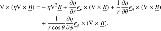 (A.2)
(A.2)
It is useful to introduce the radial, meridional, and zonal magnetic diffusivity scale heights:
 (A.3)
(A.3)
These scales can be used to evaluate whether horizontal gradients can be neglected relative to the radial one. The calculated scale heights from the model atmosphere showed that the horizontal scale heights dominate the radial scale height (i.e.,  ) and therefore horizontal diffusivity gradients in Eq. A.2 can be neglected. In order to estimate the relative importance of the advective (first term on the right-hand side of Eq. A.1) and diffusive terms (second term on the right-hand side of Eq. A.1) the magnetic Reynolds number RM is used for dimensional analysis. The typical length scale for RM has to be chosen carefully (see therefore, e.g., Liu et al. 2008 and Perna et al. 2010a). The pressure scale height
 ![Mathematical equation: ${H_p} = {{{R_d}{T_{{\rm{gas }}}}} \over g}[{\rm{m}}]$](/articles/aa/full_html/2026/04/aa58210-25/aa58210-25-eq126.png) is smaller than Hη,r for most of the upper model atmosphere (pgas < 0.1 bar) and similar in magnitude in the lower atmosphere, therefore Hp is used to calculate the magnetic Reynolds number:
is smaller than Hη,r for most of the upper model atmosphere (pgas < 0.1 bar) and similar in magnitude in the lower atmosphere, therefore Hp is used to calculate the magnetic Reynolds number:
 (A.4)
(A.4)
Note that RM may exceed unity in the model atmosphere showing that this approach is not suitable to model such hot atmospheres. When RM ≪ 1, the system is in quasi-steady-state and time derivatives can be neglected (∂t = 0). Assuming negligible dynamo action, the magnetic field is decomposed into a dipolar background  and an induced component (
 ; see, e.g., Batygin and Stevenson 2010):
 (A.5)
(A.5)
Since the induced field is typically small when RM ≪ 1, the induction equation is linearized around the background field:
 (A.6)
(A.6)
Using Ampère’s law  , the induction equation becomes
 (A.7)
(A.7)
Focusing on the zonal (ϕ) component and assuming dominant horizontal currents (i.e., jr ≪ jθ), the dominant balance becomes
 (A.8)
(A.8)
Integrating over radius from the layer of interest to the model top at radius R, an expression for the meridional current is obtained:
 (A.9)
(A.9)
The first term on the right-hand side is a boundary current in the uppermost modeled level and is set to zero for simplicity (Perna et ail 2010). Furthermore, it is assumed that the radial length scale of diffusivity variations (Hη(r)), is smaller than the characteristic meridional length scales of the zonal wind and magnetic field. As a result, radial gradients dominate over meridional ones, allowing to neglect  terms in comparison to ∂/∂r in the equation above. Assume that
  slowly varies with radius and that the atmosphere is very thin compared to the radius of the planet, then it can be approximated by
 (A.10)
The resulting Lorentz force appears in the zonal momentum equation (where for the mass density ρ the neutral gas mass density ρn was assumed) as
 (A.11)
Substituting the idealized expression for the meridional current jind,θ = −vϕBdip,r/(µ0η) gives a drag force proportional to the zonal wind velocity:
 (A.12)
Assuming a dipolar field with radial component  the equation becomes
 (A.13)
Furthermore, the magnetic field strength is assumed to be independent of radius, simplifying the radial variation of τdrag. This yields a magnetic drag timescale of the form
 (A.14)
τdrag3 is used in this study for the "active drag" treatment. Note that this approach differs from the parametrized model used in Rauscher & Menou (2013) and Beltz et al. (2022b), where the drag force is based on local flow geometry, magnetic field strength, and diffusivity via
 (A.15)
The latitudinal dependence of the radial magnetic flux density is not fully maintained in their formulation of the drag timescale and interprets drag as being proportional to the component of the wind perpendicular to the magnetic field lines. At the equator (θ = 0◦), the magnetic drag vanishes (τdrag = τdrag,Perna → ∞).
The energy equation is also modified by the kinetic energy which is lost due to the magnetic drag and returned to the atmosphere in form of localized ohmic heating with
 (A.16)
While the active drag approach is more physically motivated than the empirical Rayleigh drag, it is still an approximation. In particular, the assumption of dominant zonal winds, weak induced fields, and RM ≪ 1 may not hold in all regions of the atmosphere as shown for WASP-18 b. However, this model was still used for simulations of (U)HJs where the condition of RM ≪ 1 was not given (e.g., Beltz et al. 2022b; Coulombe et al. 2023).
A.1 Thermal ionization
Due to extreme temperatures on the dayside (> 3000 K), thermal collisions are sufficiently energetic to ionize atoms and molecules and form an ionosphere. Thermal ionization rather than photoionization is the dominant process creating strong ionospheric effects in our model, influencing the atmospheric dynamics and magnetic interactions. However, Koskinen et al. (2014) showed that photoionization can dominate over thermal ionization on the dayside atmosphere above the 100 mbar level. In order to determine the thermal ionization fraction xe,Saha in a gas in LTE, models of Menou (2012), Rauscher & Menou (2013) and others adopted the approximate solution of the Saha equation from Sato (1991). Furthermore, they assumed that the ionization fraction is small (xe,Saha ≪ 1). Therefore, only single ionization from the ground state is considered (Menou 2012). The Saha equation for a plasma in thermodynamic equilibrium is given by
 (A.17)
with the electron mass me [kg], the Boltzmann’s constant ![Mathematical equation: ${k_B}\left[ {{J \over K}} \right]$](/articles/aa/full_html/2026/04/aa58210-25/aa58210-25-eq147.png) , the gas temperature Tgas [K], the reduced Plank’s constant ℏ[Js], the electron number density ne [m−3], the ionized number density of the jth chemical species
, the gas temperature Tgas [K], the reduced Plank’s constant ℏ[Js], the electron number density ne [m−3], the ionized number density of the jth chemical species ![Mathematical equation: $n_{i,j}^ + \left[ {{{\rm{m}}^{ - 3}}} \right]$](/articles/aa/full_html/2026/04/aa58210-25/aa58210-25-eq148.png) , the atom number density nn,j [m−3] of the jth species, their partition functions Zi,j and Zn,j, and the first ionization potential Ii,j [J] of the jth species. For the calculation of xe the first 28 elements from the periodic table (hydrogen to nickel) are taken into account (Menou 2012; Rauscher & Menou 2013). The first ionization potential Ii,j ranges from 7×10⁻¹⁹ J (for K) to 4×10⁻¹⁸ J (for He) The partition functions Zi,j and Zn,j depend on the temperature in a complex way (Sato 1991). For simplicity, Zi,j and Zn,j are set to unity according to Menou (2012) since the specific atmospheric composition is unknown. Menou (2012) and Rauscher & Menou (2013) use a sum of approximate Saha expressions across multiple elements. They evaluate ionization fractions for each element
, the atom number density nn,j [m−3] of the jth species, their partition functions Zi,j and Zn,j, and the first ionization potential Ii,j [J] of the jth species. For the calculation of xe the first 28 elements from the periodic table (hydrogen to nickel) are taken into account (Menou 2012; Rauscher & Menou 2013). The first ionization potential Ii,j ranges from 7×10⁻¹⁹ J (for K) to 4×10⁻¹⁸ J (for He) The partition functions Zi,j and Zn,j depend on the temperature in a complex way (Sato 1991). For simplicity, Zi,j and Zn,j are set to unity according to Menou (2012) since the specific atmospheric composition is unknown. Menou (2012) and Rauscher & Menou (2013) use a sum of approximate Saha expressions across multiple elements. They evaluate ionization fractions for each element  independently using uncoupled Saha equations. The total number density of the jth element is given by
  . They assume that only the jth species contributes to the electrons and therefore use
  , which is not mathematically consistent, but here a useful simplification in a weakly ionized plasma in order to derive xe,Saha. The Saha equation (Eq. A.17) can be described in terms of the ionization fraction for each ion species:
 (A.18)
where  is the number density of the element j, which is calculated by assuming solar abundance (aj) for element j and the hydrogen abundance (aH), nn is the total number density of the neutrals. The numbers for the solar abundances were taken from Asplund et al. (2021). Then the total ionization fraction can be described as
 (A.19)
with the total number density of atoms/particles in all ionization states (not including electrons as independent atoms):
 (A.20)
It was assumed here that the plasma is weakly ionized  . Note that Eq. A.18 is slightly different from the derived equations in, for example, Rauscher & Menou (2013).
A more self-consistent treatment of the ionization balance is adopted for the anisotropic drag formulation using the GGchem model, compared to the approximation used by Rauscher & Menou (2013, see Sect. 4.2). The difference between the two approximations (simplified Saha and GGchem approximation) is small for pgas < 0.03 bar, deeper in the atmosphere it starts to deviate with the largest deviation around 6 bar by a factor larger than 10 for the GGchem approach.
A.2 Magnetic diffusivity
The calculation of the ionization fraction xe allows to evaluate the magnetic diffusivity η in the atmosphere via (Perna et al. 2010a; Menou 2012)
![Mathematical equation: $\eta = {1 \over {{\mu _0}{\sigma _}}} \approx 0.023{{\sqrt {{T_{{\rm{gas}}}}} } \over {{x_e}}}\left[ {{{\rm{m}}^2}{{\rm{s}}^{ - 1}}} \right].$](/articles/aa/full_html/2026/04/aa58210-25/aa58210-25-eq157.png) (A.21)
(A.21)
This expression was derived from the approximated momentum transfer due to collisions between the electrons and the neutrals with the collision rate (Draine et al. 1983)
![Mathematical equation: ${\langle \sigma v\rangle _e} \approx {10^{ - 19}}\sqrt {{{128{k_B}{T_{{\rm{gas}}}}} \over {9\pi {m_e}}}} \left[ {{{\rm{m}}^3}{{\rm{s}}^{ - 1}}} \right].$](/articles/aa/full_html/2026/04/aa58210-25/aa58210-25-eq158.png) (A.22)
(A.22)
The σ∥ was determined by
![Mathematical equation: ${\sigma _} = {{{n_e}{e^2}} \over {{m_e}{n_n}{{\langle \sigma v\rangle }_e}}}\left[ {{\rm{S}}{{\rm{m}}^{ - 1}}} \right].$](/articles/aa/full_html/2026/04/aa58210-25/aa58210-25-eq159.png) (A.23)
(A.23)
Appendix B Alternative derivation of the anisotropic drag
The model of Christie et al. (2025) extends the active drag model of Perna et al. (2010a) and derives an approximation of the Lorentz force which includes both the Pedersen and Hall effect through anisotropic conductivities. The drag force is expressed in terms of the anisotropic ionospheric conductivities for ions and electrons:
 (B.1)
(B.1)
with the Pedersen (σP) and Hall conductivities (σH) for plasma consisting of one ion and electron species:
 (B.2)
(B.2)
 (B.3)
(B.3)
For the parameter regime used for WASP-18 b simulations, the ionospheric conductivities can be approximated by σH ≈ σH,e and σP ≈ σP,e. For the parameters used here, the comparison between the factors in Eqs. B.1 and 36 shows that they are the same in magnitude, i.e.,  and
and  . The main difference between this approach and the parametrized anisotropic drag presented in Sect. 4 is the physical origin of the drag term. In Sect. 4, the magnetic drag exerted on the neutrals is directly calculated from the collisional momentum transfer between the plasma and the neutral fluid, whereas the method of Christie et al. (2025) describes the Lorentz force acting on the plasma fluid, which is then balanced by the drag force exerted by the neutrals. The method to parametrize the collisional drag force on the neutrals via the differential velocities
  is more direct, since the Lorentz force does not appear in the neutral momentum equation (Eq. 24). Neutrals experience magnetic effects only though collisions with the charged species. Furthermore, Christie et al. (2025) include both horizontal and vertical components of the magnetic drag force in their non-hydrostatic model, whereas in this work the vertical drag component is neglected since a hydrostatic framework in the vertical direction is applied. However, note that in Eq. B.1 the conventional conductivities are defined in the plasma’s rest frame (Eqs. B.2 and B.3). In order to use it in the neutral gas’s rest frame, the conductivities have to be transformed into effective conductivities which are more complex and are given in Sect. 4 of Song et al. (2001). However, the effective conductivities become the same as the conventional conductivities (here σH ≈ σH,e and σP ≈ σP,e) under the following approximations (Song et al. 2001): νinνen ≫ ωiωe, νen ≫ ωe, and negligible collisions between electrons and ions. For the parameter regime on the dayside of the simulations WASP-18 b these conditions are fulfilled and the drag formulation in Eq. B.1 is a suitable approach for the magnetic drag to be applied in ExoRad. The energy equation is accordingly modified with the heating rate:
 (B.4)
(B.4)
Appendix C Comparison of different ion-neutral drift velocities
As already pointed out by Christie et al. (2025) the relative velocity between ions and neutrals in the atmosphere derived using the anisotropic drag approach differs from that applied in the toy model of Savel et al. (2024). While the drift velocity between ions (index s = i) and neutrals is given in Eq. 31, Savel et al. (2024) assumes that the conductivity tensor can be expressed as a scalar in this system and therefore applies the approach from Perna et al. (2010a) for the meridional current density jind,θ ∼ vϕBdip/(µ0η) resulting in a different drift velocity:
 (C.1)
(C.1)
In this approach, the assumed electrical conductivity is the parallel conductivity (Eq. A.23). This value begins to deviate from the Pedersen conductivity above the M1 region (see Fig. 4 in Koskinen et al. 2014 or Fig. 2 in Christie et al. 2025) leading to larger drift velocities in the Savel et al. approach. The M1 region is defined as the area where particles are not coupled to the magnetic field lines and both ion and electron magnetizations (Eq. 21) satisfy ki, ke ≪ 1. A discussion on the differences of the two different approaches is given in Christie et al. (2025). Figure C.1 compares the approximated ion–neutral drift velocities derived in this work with those predicted by the approach of Savel et al. (2024). Both approaches show a similar monotonic increase in drift speed with decreasing pressure, indicating that collisional coupling becomes weaker as the density decreases. However, the Savel et al. approach predicts larger drift velocities by up to several orders of magnitude for pgas ≤ 10−4 bar, the pressures which are generally probed in high-resolution transmission spectroscopy (Savel et al. 2024). The simulation domain extends up to pressures of pgas ∼ 10−4 bar. Extrapolating the derived ion–neutral drift to lower pressures suggests that relative velocities could reach values of order km s−1, and may therefore be detectable with high-resolution spectroscopy in the photosphere. The equatorial  profile behaves differently from higher latitudes due to the dipolar magnetic field geometry, where the radial magnetic field vanishes at the equator and the ion–neutral drift velocity is purely zonal. The differences in the profiles and approaches highlight the magnetic field geometry dependence. Differences also occur between the morning and evening terminators due to the feedback of the anisotropic drag on the atmospheric flow velocity. These dependences emphasize the need for accurate physical models to interpret ion–neutral drift measurements and to constrain exoplanetary magnetic field strengths.
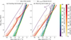 |
Fig. C.1 Ion–neutral drift velocities as a function of pressure and latitude at the evening terminator (a): ϕ = 90◦) and morning terminator (b): ϕ = −90◦) for two different approaches. Solid lines show |

It is the temperature that a gas volume would attain under adiabatic expansion/compression if the gas would be brought to a reference pressure, which is here set to the pressure of the lower boundary equal to 700 bar.
For most molecules, opacities are taken from the ExoMol data base (Tennyson et al. 2016, 2020).
Due to the quadratic dependence on the radial magnetic field component  , the drag timescale τdrag is insensitive to whether the dipole magnetic field is aligned or anti-aligned with the rotation axis.
All Tables
Physical (top) and numerical (bottom) parameters for WASP-18 b ExoRad simulations.
ExoRad results: Effect of magnetic drag on WASP-18 b’s climate state characteristics.
All Figures
|
Fig. 1 (a) Spatial variations in magnetic Reynolds number (RM (Eq. (22)), left) and (b) thermal ionization fraction (xe, right) for WASP-18 b. Large areas of the dayside are in the intermediate and high-RM regimes, while ionization varies over many orders of magnitude, motivating an anisotropic drag treatment that accounts for local conductivity and magnetic geometry. The lines show gas temperature-pressure profiles averaged over all latitudes and over different regions in the atmosphere: dayside (−90◦< ϕ ≤ 90◦), nightside (|ϕ| > 90◦), morning (−97.5◦≤ ϕ ≤ −82.5◦) and evening terminator (82.5◦≥ ϕ ≥ 97.5◦). The results of the simulation with anisotropic drag were used in the calculation of RM, xe, and the averaged temperature-pressure profiles shown here. |
| In the text | |
|
Fig. 2 Magnetization parameter (Eq. (21)) profiles for ions (ki) and electrons (ke) averaged over all latitudes and over dayside atmosphere (−90◦< ϕ ≤ 90◦). The dotted blue line (ωpe/νen) shows the relation between the electron plasma frequency and the electron–neutral collision frequency averaged over the dayside atmosphere. The plasma coupling ratios were calculated from the ExoRad simulation for WASP-18 b with anisotropic drag. The dashed gray line shows where the plasma coupling ratio reaches unity. |
| In the text | |
|
Fig. 3 Hall (KH,s) and Pedersen (KP,s) drag coefficients for electrons (s = e) and ions (s = i) averaged over all latitudes and over dayside atmosphere (−90◦< ϕ ≤ 90◦). KH = KH,i − KH,e and KP = KP,i + KP,e are the total Hall and Pedersen coefficients. The coefficients were calculated using the gas pressure-temperature profile from the ExoRad simulation run of WASP-18 b with anisotropic drag. The gray line shows KP obtained directly from ExoRad. It diverges from the calculated KP (blue line) in the upper atmosphere because the drag timescale in ExoRad is limited to τdrag ≥ 100 s. The same applies for KH from ExoRad (not shown here). |
| In the text | |
|
Fig. 4 Maps of horizontal wind speed |vh| and streamlines (white lines) at two pressure levels (pgas =0.1 bar and pgas =0.001 bar) for the four different magnetic drag treatments (no drag, uniform drag, active drag, and anisotropic drag). The substellar point is centered at each map. The vertical dashed black lines mark the area at longitude ±90◦. The output of each velocity component is time-averaged over 100 days of simulation time to eliminate the small-scale fluctuations. |
| In the text | |
|
Fig. 5 Mean zonal wind for the four different magnetic drag treatments in different regions of the atmosphere: dayside atmosphere (first row), nightside atmosphere (second row), and total atmosphere (third row). The zonal wind velocity, u, is averaged at a specific latitude, and pressure level across longitudes on the dayside (−90◦≤ ϕ ≤ 90◦), on the nightside (|ϕ| > 90◦), and all longitudes. The black line shows the zero-wind contour, the boundary between super-rotation and counter-rotation. The output of the zonal wind velocity is time-averaged over 100 days of simulation time to eliminate the small-scale fluctuations. |
| In the text | |
|
Fig. 6 Maps of gas temperature and velocity field at two gas pressure levels (pgas = 0.1 bar and pgas = 0.001 bar) for the four different magnetic drag treatments. The substellar point is centered at each map and is marked with a white star. The velocity field is shown by the white arrows. The length of the arrow scales with the relative wind velocity. The vertical dashed black lines mark the area at longitude ±90◦. The cyan contours represent the hotspot region (Tgas,max, Tgas,max − 1K) with Tgas,max being the largest temperature for the chosen pressure level. The temperature is time-averaged over 100 days of simulation time to eliminate the small-scale fluctuations. |
| In the text | |
|
Fig. 7 Gas temperature-pressure profiles for four different drag treatments averaged over all latitudes and over different regions in the atmosphere: dayside (−90◦< ϕ ≤ 90◦), nightside (|ϕ| > 90◦), morning terminator (−97.5◦≤ ϕ ≤ −82.5◦), and evening terminator (82.5◦≥ ϕ ≥ 97.5◦). All drag treatments show pronounced day-night differences and temperature inversions in the upper atmosphere. Nightside temperatures are cooler when active or anisotropic magnetic drag is applied compared to no drag. |
| In the text | |
|
Fig. 8 Diffusion coefficients from the Ohm’s law (Eq. (6)) averaged over all latitudes and over dayside atmosphere (−90◦< ϕ ≤ 90◦). The coefficients were calculated from the output of the ExoRad simulation with anisotropic drag for the atmosphere of WASP-18 b. |
| In the text | |
|
Fig. C.1 Ion–neutral drift velocities as a function of pressure and latitude at the evening terminator (a): ϕ = 90◦) and morning terminator (b): ϕ = −90◦) for two different approaches. Solid lines show |
| In the text | |
Current usage metrics show cumulative count of Article Views (full-text article views including HTML views, PDF and ePub downloads, according to the available data) and Abstracts Views on Vision4Press platform.
Data correspond to usage on the plateform after 2015. The current usage metrics is available 48-96 hours after online publication and is updated daily on week days.
Initial download of the metrics may take a while.