| Issue |
A&A
Volume 708, April 2026
|
|
|---|---|---|
| Article Number | A267 | |
| Number of page(s) | 21 | |
| Section | Stellar structure and evolution | |
| DOI | https://doi.org/10.1051/0004-6361/202558301 | |
| Published online | 14 April 2026 | |
Spectral dataset of stripped-envelope supernovae from the Tsinghua supernova group
1
Beijing Planetarium, Beijing Academy of Sciences and Technology, Beijing, 100044, China
2
Department of Physics, Tsinghua University, Haidian District, Beijing, 100084, China
3
Yunnan Observatories, Chinese Academy of Sciences, Kunming, 650216, China
4
International Centre of Supernovae, Yunnan Key Laboratory, Kunming, 650216, China
5
Key Laboratory for the Structure and Evolution of Celestial Objects, Chinese Academy of Sciences, Kunming, 650011, China
6
School of Physics and Information Engineering, Jiangsu Second Normal University, Nanjing, Jiangsu, 211200, China
7
Institute for Frontiers in Astronomy and Astrophysics, Beijing Normal University, Beijing, 102206, China
8
Key Laboratory of Space Astronomy and Technology, National Astronomical Observatories, Chinese Academy of Sciences, 20A Datun Road, Beijing, 100101, China
9
School of Astronomy and Space Science, University of Chinese Academy of Sciences, Beijing, 100049, China
10
National Astronomical Observatories, Chinese Academy of Sciences, Beijing, 100101, China
11
School of Science, Tianjin University of Technology, Tianjin, 300384, China
12
Department of Astronomy, Shanghai Jiao Tong University, Shanghai, 200240, China
13
Department of Astronomy, University of Science and Technology, Hefei, 230026, China
14
School of Physics and Astronomy, Beijing Normal University, Beijing, 100875, China
15
Key Laboratory of Optical Astronomy, National Astronomical Observatories, Chinese Academy of Sciences, Beijing, 100101, China
16
Schools of Electronics and Information Engineering, Wuzhou University, Wuzhou, 543002, China
17
Institute for Frontiers in Astronomy and Astrophysics, Beijing Normal University, Beijing, 102206, China
18
Department of Astronomy, School of Physics and Astronomy, Yunnan University, Kunming, 650091, China
19
Department of Astronomy, School of Physics, Peking University, Beijing, 100871, China
20
College of Physics, Guizhou University, Guiyang, 550025, China
★ Corresponding authors: This email address is being protected from spambots. You need JavaScript enabled to view it.
; This email address is being protected from spambots. You need JavaScript enabled to view it.
; This email address is being protected from spambots. You need JavaScript enabled to view it.
Received:
28
November
2025
Accepted:
9
March
2026
Abstract
Context. The extent of envelope stripping in progenitor stars is directly reflected in the diversity of spectral features that are observed in stripped-envelope supernovae (SESNe).
Aims. Through extensive spectral observation and analysis, we aim to clarify the statistical differences between the subclasses of SESNe.
Methods. The Tsinghua supernova group obtained 249 optical spectra of 62 SESNe from 2010 to 2020, covering phases from –16 to over 190 days relative to maximum light. Most spectra were obtained during the photospheric phases after the supernova explosion. For each spectrum, the pseudo-equivalent widths and blueshift velocities of the principal lines were measured. We further investigated the common spectral features by analyzing their velocity and strength correlations across all subtypes.
Results. We identified the feature near 6200 Å in SNe Ib as Hα through a comparison with SNe IIb and Ic. This resolves inconsistent interpretations in the literature. Our finding reveals prevalent residual hydrogen in SNe Ib, further supporting a continuous stripping sequence from SNe IIb to Ib. The velocity among different subtypes of stripped-envelope SNe increases, with SNe IIb exhibiting the lowest line velocities, followed by Ib, Ic, and Ic-BL. Typically, the O I lines in SNe Ic/Ic-BL are stronger than those seen in SNe IIb/Ib. In nebular phases, the [Ca II] emission dominates [O I] in SNe IIb/Ib, while [O I] is stronger in SNe Ic, including in the He-rich SN 2016coi. This spectral dichotomy implies that progenitors of SNe Ic (BL) have more massive CO cores and hence higher initial masses.
Key words: methods: data analysis / techniques: spectroscopic / stars: massive / supernovae: general
© The Authors 2026
 Open Access article, published by EDP Sciences, under the terms of the Creative Commons Attribution License (https://creativecommons.org/licenses/by/4.0), which permits unrestricted use, distribution, and reproduction in any medium, provided the original work is properly cited.
This article is published in open access under the Subscribe to Open model. This email address is being protected from spambots. You need JavaScript enabled to view it. to support open access publication.
1. Introduction
Core-collapse supernovae (CCSNe) are the violent deaths of massive stars with initial masses ≳8 M⊙. During the evolution of massive stars, their envelope materials may be stripped by stellar winds, binary interaction, or eruptive mass ejection. Therefore, at the moment of explosion, the stars become H poor or even He poor, and thus, the corresponding spectral features in the SN spectra also decrease (Filippenko 1997; Gal-Yam 2017). These SNe are classified as stripped-envelope supernovae (SESNe). The spectra of SNe IIP/IIL or IIn exhibit persistent H lines, whereas in SNe IIb, the H lines weaken and eventually fade, and He I lines progressively become the dominant feature. Weaker H lines indicate that the H envelope in SN IIb progenitors has been partially stripped. SNe Ib lack H lines, but show strong He lines, indicating that their progenitors have lost their H envelopes, but still retain their He envelopes. The spectra of SNe Ic lack H and He lines, implying that the H and He envelopes of their progenitors have both been lost before the explosion.
During the past decade, a new class of peculiar SN that is spectroscopically similar to SESN was discovered. Their observed properties are best explained by the ultra-stripped supernova model (Tauris et al. 2015; Yao et al. 2020; Yan et al. 2023; Das et al. 2024). These events are characterized by fast-evolving light curves, which imply unusually low ejecta masses and extensive stripping of the progenitor material. Observations indicate that several such SNe have likely lost their C/O layers (Kuncarayakti et al. 2022; Gal-Yam et al. 2022; Pellegrino et al. 2022; Nagao et al. 2023; Wu et al. 2024), even the inner O/Si/S layers (Schulze et al. 2025).
In classical stellar evolutionary theories in which stars evolve alone, stars with MZAMS ≳ 25 M⊙ can evolve to H-poor Wolf-Rayet stars and explode as SNe Ib or Ic. However, there is no consensus about whether SESNe are produced by single stars or binaries, nor about the mass range of the progenitors. However, mounting evidence now favors lower-mass binary systems over very massive single stars as the dominant formation channel for SESNe (Sana et al. 2012; Yoon 2015; Prentice et al. 2019; Zapartas et al. 2025). The few studies based on direct observations of SN IIb or Ib progenitors to date have favored progenitors of lower initial masses in binary systems. For instance, strong evidence indicates a companion for the progenitor of SN Ib iPTF13bvn (Cao et al. 2013; Bersten et al. 2014; Eldridge et al. 2015; Kuncarayakti et al. 2015; Eldridge & Maund 2016). Similarly, a yellow hypergiant companion has been suggested for SN 2019yvr (Kilpatrick et al. 2021; Sun et al. 2022). No direct detection of SNe Ic progenitors has been reported to date, even though indirect evidence of binary companions has been found (Xiang et al. 2019; Fox et al. 2022; Zhao et al. 2025). The most massive stars with MZAMS ≳ 25 M⊙ may instead result in superluminous SNe or failed SNe. Moreover, binary progenitors have also been proposed to contribute to the diversity of H-rich SNe II (Podsiadlowski 1992; Zapartas et al. 2019), suggesting that this channel may be common for all types of core-collapse supernovae.
One way to study the properties of SESN progenitors is through their spectra. The spectral line intensities during the photospheric phase reflect the envelope composition, providing insight into the extent of envelope stripping prior to the explosion. Additionally, in the nebular phase, luminosity ratios of [O I] and [Ca II] lines are strongly correlated with the progenitor CO core masses (Jerkstrand et al. 2014, 2015; Dessart et al. 2021; Fang et al. 2019; Fang & Maeda 2023). Models of nebular spectra also show that higher L[OI] and L[NII] correspond to higher initial masses. Through spectroscopic observations and large-sample statistical analysis, it is possible to clarify the differences in envelope stripping among progenitor stars of different types of SESNe. This approach can address questions such as whether the degree of envelope stripping in progenitor stars of SNe with different spectral types is continuous or distinct across spectral types, how the composition of the remaining envelope affects the spectrum characteristics, and so on.
Substantial optical spectroscopic databases for SESNe now comprise over 2500 spectra for objects discovered between 1994 and 2016 (Modjaz et al. 2014; Fremling et al. 2018; Shivvers et al. 2019; Stritzinger et al. 2023). These data facilitate a more accurate classification, reveal the ejecta composition across subtypes, and probe progenitor properties Liu et al. (2016), Shivvers et al. (2019), Fremling et al. (2018). Although the classifications of SESNe are based on the presence or absence of several specific lines, some SNe show spectral evidence of residual hydrogen in SNe Ib (e.g., Modjaz et al. 2014) or helium in SNe Ic (e.g., Drout et al. 2016; Prentice et al. 2018). Hydrogen features are now considered common in SNe Ib. The comparison of spectra near maximum light of SNe IIP, IIb, and Ib shows a sequence of increasing prominence of He I lines and decreasing H I line strength (Gal-Yam 2017). Moreover, measurements of spectral lines reveal a continuous variation in the Hα line strength from SNe IIb to Ib, suggesting that envelope stripping in their progenitors may be a gradual process. In contrast, the photospheric spectra of SNe Ic are distinct from those of SNe IIb and Ib, favoring models with negligible helium over those with gradually stripped He envelopes (Liu et al. 2016; Fremling et al. 2018). Furthermore, nebular-phase spectroscopic analysis reveals that while SNe IIb and Ib share similar CO core-mass distributions, SNe Ic show significantly higher CO core masses, implying more massive progenitor stars Fang et al. (2019). These observational studies appear to confirm that progenitor stars of SNe Ic have completely lost their He envelopes. Although some theoretical studies ruled out substantial residual He in SNe Ic (Frey et al. 2013; Williamson et al. 2021), others proposed that mixing of He might affect the spectral types of SNe Ib/c, and thus, He might be hidden in SNe Ic (Dessart et al. 2012). Determining the true stripping history of SESNe progenitors thus requires further observations and theoretical modeling.
We present the spectra of SESNe obtained by the supernova group at Tsinghua University (THU). A total of 249 low-resolution spectra were obtained for 62 SNe from late 2010 to 2020. Our database extends the temporal coverage of previous homogeneous samples by including SNe up to 2020, compared to the 2016 cutoff in earlier works. A portion of spectra from our group have been published in Lin et al. (2024) for SNe II and in Li et al. (2021) for some SNe Ia. All spectral data we used are available via the Weizmann Interactive Supernova Data Repository (WiseREP1; Yaron & Gal-Yam 2012).
2. Observations
Since 2010, the supernova group at THU has been conducting continuous observations of SNe, including multiband photometry and spectroscopy in optical wavelengths. Optical spectra of SNe were obtained using the Beijing Faint Object Spectrograph and Camera (BFOSC) or the spectrograph made by Optomechanics Research Inc. (OMR), mounted on the 2.16 m telescope at Beijing Xinglong Observatory (BAO) (hereafter XLT; Fan et al. 2016) and the Yunnan Faint Object Spectrograph and Camera (YFOSC) on the 2.4 m telescope at Lijiang Observatory (hereafter LJT; Fan et al. 2015). We selected recently discovered supernova candidates from public databases such as the latest supernovae website2 and the transient name server (TNS3). To ensure a good data quality, we only observed SNe or SNe candidates brighter than ∼18 mag. The two telescopes monitored low-resolution (R ∼ 500–2000) spectroscopy for SNe. All the spectra were reduced using standard IRAF pipelines (Tody 1986, 1993), including bias and flat-field corrections. The wavelength calibration solution was determined using the arc lamps of He/Ar or Fe/Ar and was applied to the one-dimensional spectra. The flux calibrations were obtained using the spectra of nearby standard stars taken on the same night. Finally, telluric absorptions were removed from the spectra using the atom lines produced by the reduction process.
For some SNe, photometry was conducted in Johnson-Cousins BVRI or BV plus Sloan gri bands with the 80 cm THU-NAOC Telescope (TNT; Wang et al. 2008; Huang et al. 2012) at BAO. The TNT light curves were used to derive the date of maximum light when available.
Through a decade-long observational campaign conducted from 2010 to 2020, we ultimately obtained a total of 249 spectra of 62 SESNe. The details of these SNe and of the corresponding observations are listed in Tables A.1 and A.2, respectively. As a summary, 106 spectra are from XLT and 139 are from LJT. Spectroscopic data for 8 SNe were previously published in separate papers (see details in Table A.2). These published data include 4 additional spectra for SN 2017ein from telescopes outside China, including the 2 m Faulkes Telescope North (FTN) of the Las Cumbres Observatory network, the 9.2 m Hobby-Eberly Telescope (HET), and the ARC 3.5 m telescope at Apache Point Observatory (hereafter APO-3.5 m). These spectra are also included in this work. Specifically, the spectra for 7 SNe (CSS141005, PSN J0123, SNe 2010ln, 2011bl, 2012C, 2012ej, and 2017iro) are presented here for the first time. Furthermore, only the classification spectra for the spectral data for 8 SNe (2016bll, 2016cce, 2016G, 2016M, 2017cxz, 2017jdn, 2018ie, and 2018if) are publicly available on TNS, and all originate from our research group.
Fig. 1 show the pie chart of the observed SNe and the spectra by type. The number of SNe Ib is comparable to that of SNe Ic, and it is approximately twice that of SNe Ic-BL. The local rate of different subtypes of SESNe was recently presented by Ma et al. (2025b,a). We note that the type fractions of our spectral sample differ significantly from those in Ma et al. (2025b), who reported 35%, 17.5%, 32.5%, and 15% for IIb, Ib, Ic, and Ic-BL, respectively. While the fractions of Ic and Ic-BL in our sample are consistent with those in the literature, we find notable discrepancies for types IIb and Ib. This may be attributed to several factors. First, it is important to emphasize that our sample does not include a generic Ib/c subtype. First, objects classified as Ib/c on public platforms, for instance, on TNS or the Weizmann Interactive Supernova Data Repository (WiseREP; Yaron & Gal-Yam 2012), were reclassified as Ib or Ic based on detailed spectroscopic analysis (see the footnote of Table A.1). Second, Ma et al. (2025b) imposed a strict cutoff distance of 40 Mpc (z ≈ 0.01) to ensure sample completeness. However, the redshifts of 34 supernovae (∼55%) in our sample exceed 0.01, suggesting a potential bias in the sample selection. Additionally, SNe IIb have the lowest mean peak luminosity among the four subclasses (Richardson et al. 2014). Consequently, a brightness-limited spectroscopic sample might miss a substantial fraction of these dimmer events, leading to an underrepresentation of SNe IIb. Furthermore, as we discuss below, some SNe Ib also show hydrogen lines in their spectra, and SNe IIb might be misclassified as type Ib, which might also affect the observed fractions.
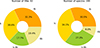 |
Fig. 1. Pie charts of the numbers of SNe (left) and numbers of spectra (right) by type. |
The right panel of Fig. 1 shows the proportions of spectra across different subtypes. The fractions of type Ib and Ic spectra are similar to the actual fractions of SN types estimated for the local Universe. The significant increase in the number of type Ic-BL spectra is likely due to the selection bias, with a tendency of obtaining more spectra for rare SN types. The relatively small number of type IIb spectra is likely due to their intrinsically lower luminosity, which makes it challenging to obtain high-quality spectra. As a result, type IIb SNe are often deprioritized as observational targets, or the obtained spectra exhibit excessively low signal-to-noise ratios.
In Fig. 2 we show the distribution of SN redshift, the number of spectra for each SN, the phases of the spectra, and the phases of the first spectrum for an SN. The SNe of our spectral sample have an average redshift of 0.015, with the maximum redshift being 0.06 (SN 2018beh). Most SNe of our sample were observed only once, and an average of four spectra were obtained for each SN.
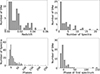 |
Fig. 2. Distribution of the SN redshift (upper left panel), number of spectra for a single SN (upper right panel), phases of spectra (lower left panel), and the phase of the first spectrum of each SN (lower right panel). |
3. Spectral analysis methods
Several groups previously published spectroscopic samples of SESNe, including Modjaz et al. (2014) from the Harvard-Smithsonian Center for Astrophysics, Fremling et al. (2018) from the Palomar Transient Factory, Shivvers et al. (2019) from the Lick Observatory Supernova Search collaboration of Berkeley, and Stritzinger et al. (2023) from the Carnegie Supernova Project. The relevant analysis papers include Modjaz et al. (2016), Liu et al. (2016), Williamson et al. (2019), and Holmbo et al. (2023). The subsequent analyses of these samples commonly involve measuring line velocities and intensities, comparing spectral properties across subtypes, and applying principle component analysis (PCA) for classifications. Our analysis references and builds upon this body of work.
3.1. Preprocessing the spectra
The original SN spectra, obtained from different instruments under varying conditions, have a different wavelength resolution and signal-to-noise ratios. To enable a consistent comparison, we homogenized the dataset by convolving all spectra to a common resolution and applying a smoothing kernel. Fig. 3 shows the procedure of spectrum preprocessing. First, the observed wavelengths were converted into the rest frame by dividing (1 + z), where z is the SN redshift. Following Blondin & Tonry (2007), we then binned the wavelength axis logarithmically with dλln = 0.0015, corresponding to dλ = 10 Å (dv = 450 km s−1) at Hα. For spectra containing strong host-galaxy emission lines, emission lines were masked out by applying a third-order polynomial fit to the adjacent continuum. Then, the binned spectra were smoothed with a Savitzky-Golay filter using the Python function scipy.signal.savgol_filter. Finally, spectra in photospheric phases were normalized by fflat = fobs/fcon − 1, where fflat is the normalized flux, and fcon is the pseudo-continuum. To calculate the pseudo-continuum, we first chose a certain number of knots and calculated the mean flux between each pair of knots. Then, we fit the knots with a smoothing spline fit using the Python function scipy.interpolate.UnivariateSpline.
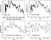 |
Fig. 3. Preprocessing method for our spectral data. (a) Input spectrum after corrections of redshift. (b) Spectrum after binning into logarithmic scale with dλln = 0.0015. (c) Smoothed spectrum with a window length of 21. The pseudo-continuum is plotted as a dotted line. (d) Spectrum normalized by dividing the continuum in (c). |
3.2. Determining dates of maximum light
To determine the phase of each spectrum, the time of maximum light of each SN is needed. We first checked the light curves by TNT and found 14 SNe in our sample have abundant photometric observations around the peak in B- or V-band. For the remaining SNe, we collected light-curve data from the literature and open data archives such as the Zwicky Transient Facility (ZTF; Masci et al. 2019; Bellm et al. 2019). When only ZTF gr-band photometry was available, we converted the Sloan magnitudes into standard Johnson BV-band magnitudes by applying the relation presented by Jordi et al. (2006). The dates of maximum light were then estimated using a third-order polynomial fit to the light-curve data around peak. Using this approach, we determined the time of maximum light for 41 SNe in total.
For SNe without sufficient light-curve data, we used SNID (Blondin & Tonry 2007) to determine the phase via a spectral cross correlation, thereby estimating the date of V-band maximum. This method yielded peak dates for 21 SNe in our sample. All derived times of maximum light are listed in Table A.1. As shown in Fig. 4, most SESNe reached the V-band peak 2.2 ± 1.2 days after the B-band peak, consistent with the finding of Brown et al. (2014). Therefore, for SNe with a valid estimate of peak dates in the B band alone, we estimated the peak dates in V band by adding an average offset of 2.2 days. This approach was used for 3 SNe in our sample. Throughout this work, phases are the rest-frame days since V-band maximum to match the convention used by SNID.
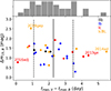 |
Fig. 4. Distribution of tmax, V − tmax, B vs. Δm15, B of our SESN sample. The vertical lines mark the average delay (solid line) and 1σ range (dashed lines). Different types are plotted in different colors, which are denoted in the upper right corner. |
Several SNe are outliers in the tmax, V − tmax, B distribution (Fig. 4), lying outside the 1σ range of the average. We found a weak negative correlation between this peak-time difference and the decline rates Δm15 in B band. Most outliers still follow the relation, except for SN 2014ad and SN 2016adj. These outliers may originate from energy sources that depart from the typical case. We note that SN 2013ge is a type Ic with double-peaked light curves (Drout et al. 2016). Two scenarios are proposed for the additional energy input of the first peak: an extended envelope, or outward mixing of 56Ni. Both scenarios would result in a faster rise in bluer bands, and therefore, in a larger separation between the B- and V-band peaks. SN 2014ad is a broad-lined type Ic that was exceptionally energetic compared to other SNe Ic-BL (Sahu et al. 2018). SN 2016adj is a carbon-rich SN Ic that exhibited CO emission two months after explosion, and hydrogen emission in the near-IR (NIR) about 3 months after explosion (Stritzinger et al. 2024, 2022; Banerjee et al. 2018). SN 2016iae is a normal SN Ic with a relatively flat velocity evolution (Prentice et al. 2019). The energy sources of SNe 2016adj and 2014ad probably differ from those of other SESNe. SN 2018gep was found to have a faster temporal evolution in the light curves. Although classified as broad-lined, SN 2018gep is an outlier when compared with other SNe Ic-BL except for iPTF16asu, which transitions from a fast blue transient to an SN Ic-BL (Pritchard et al. 2021). Its early light curve was attributed to interaction between the ejecta and circumstellar material lost through eruptive mass loss shortly before explosion (Ho et al. 2019).
3.3. Line identification and measurements
An accurate line identification is required prior to measuring line intensities and velocities. For this task, we consulted established line lists from previous studies (Liu et al. 2016; Holmbo et al. 2023) and used the spectral synthesis code SYNOW/SYNAPPS (Thomas et al. 2011) for verification.
Holmbo et al. (2023) identified the main features by fitting the mean spectra of each subtype at multiple epochs with 11 ionic species. For SNe IIb, the primary spectral features include H I, He I, O I, Na I, Fe II, Ti II, Ca II, and possibly, high-velocity Si II. For SNe Ib, the main elements are the same as for SNe IIb, with ambiguous detections of H I. For SNe Ic, the main features are identified as O I, C II, Na I, Si II, Fe II, Ti II, Co II, and Ca II. The C II lines are visible only in early phases and faded after maximum light. In our preliminary spectral fitting, we used identical ion species. Thus, the main features in our SN spectra were identified according to previous studies and our fitting results. Consequently, for all SNe, the lines of Fe II, the Ca II NIR triplet, and OI λ7774 were identified and measured. Specifically, the lines of Hα, Hβ, He Iλ5876, He Iλ6678, and He Iλ7065 were identified for SNe IIb; and the lines of He Iλ5876, He Iλ6678, He Iλ7065, and He Iλ7281 were identified for SNe Ib; the lines of Si IIλ6355, C IIλ6580, and C IIλ7234 can be identified for SNe Ic/Ic-BL in phases earlier than +10 d. For SNe Ic, which we treated as helium free, the 5700 Å absorption was interpreted as Na I D, neglecting potential contamination from He Iλ5876. The 6200 Å absorption was identified as Si IIλ6355. We note that for SNe Ib, the feature at similar wavelength can be residual H or Si II, which we discuss further in Sect. 4.
For each spectrum, we measured the pseudo-equivalent widths (pEWs) and expansion velocities of each line. The procedure was as follows. First, on the smoothed (but not normalized) spectra, we defined the wavelength range for each line by locating the local maxima flanking the absorption trough or distinct inflection points (where df/dλ ≈ 0). This range selection is illustrated in Fig. 5. We then constructed a local pseudo-continuum by drawing a straight line between the two endpoints of the defined range. Finally, the pEW was calculated by normalizing the flux within the line range to this local pseudo-continuum and integrating across the wavelength interval.
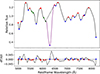 |
Fig. 5. Schematic diagram illustrating the method of defining the spectral line range. For the smoothed spectrum (upper panel), the first derivative of flux with respect to wavelength is computed (lower panel). Local maxima and minima are identified where the sign of the derivative changes, marked with red upward-pointing and blue downward-pointing triangles, respectively. At certain wavelengths, distinct inflection points are observed where the derivative approaches zero without a sign change; these are indicated by green upward-pointing triangles. The wavelength range of the Hα line is thus delineated in purple, while the local pseudo-continuum is represented by the dashed black line. |
In most cases, where a spectral line does not blend with others, its pEW was calculated by directly integrating over the wavelength interval, and the expansion velocity was taken as the blueshift of the absorption minimum, and for spectral line blending, multi-Gaussian fitting was employed to deconvolve the individual lines. The wavelength range of each blended line was defined by the intersection points of the fitted Gaussian functions, and the line velocity was determined by the blueshifted minimum of the corresponding Gaussian component. Common blends treated in this way include the O Iλ7774+Ca II NIR triplet in high-velocity SNe Ic and Ic-BL, and the Hα+He Iλ6678 complex in SNe Ib. In particular, we found that Fe II lines (λλ4924, 5018, 5091, 5169, and 5198) in most spectra are severely blended and it is challenging to separate each component (see Figs. 6 and 7 of Liu et al. 2016). To ensure uniformity and avoid inconsistencies in defining individual component boundaries, we only measured the total pEW of the blended Fe II feature. Its velocity was measured from the blueshifted minimum of the Fe IIλ5169 line on the red side of the blend. In SNe IIb, where the Fe II lines blend with Hβ, we applied multi-Gaussian fitting to separate the contributions and measure their individual pEWs.
We constructed mean spectra for each SESN subtype at various epochs using the normalized spectra. The phases were set to be in range of −10 d to +40 d, with an interval of 10 days. For each phase, we selected spectra obtained within a 5-day interval around that age. To avoid over-representing individual SN with multiple spectra, only the spectrum closest to the target phase was used from each object. At least three SNe (spectra) were required to derive the mean spectrum in a given phase. Fig. 6 shows the mean spectra of each type, with the dominant spectral features marked in different colors. As shown in Fig. 6, for each subtype, the line profiles of different SNe at the same epoch exhibit varying degrees of diversity. In SNe IIb, the Hα region and Fe II lines show greater scatter in a given phase than the He I lines. For SNe Ib, the strength of Hα displays considerable variation at early times, but eventually gradually converges. In SNe Ic, significant dispersion is present in the C II and Si II regions in the early phases; except for Fe II lines, the post-peak (≳30 days) dispersion appears to mainly arise from differences in the strength of the emission components of the lines, possibly reflecting diversity in ejecta thickness. SNe Ic-BL do not show pronounced changes in diversity across epochs, with the Si II and O I lines exhibiting the greatest variation.
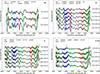 |
Fig. 6. Mean spectra and their corresponding standard deviations of different subtypes of SESNe at four different phases spanning from –10 to 40 days since V-band maximum. The numbers on the right side of each set of spectra are the corresponding phases, and number of spectra included to calculate the mean spectra is shown in the brackets. The mean spectra are shown by solid black lines, and the 1σ uncertainty is shown by shaded gray regions. Each single spectrum is plotted in light green. For each spectrum, the lines are marked by colors denoted at the top of each figure. |
Mean spectra of different subtypes at various epochs were also presented by Liu et al. (2016) and Holmbo et al. (2023). Those from the former are publicly available online. Our mean spectra show excellent agreement with theirs, particularly for types IIb and Ib, where differences are minimal (Fig. A.1). A notable discrepancy is observed for SNe IIb near maximum light: the absorption around 6900 Å (He Iλ7065) is weaker in our sample. For SNe Ic, the mean spectra also exhibit only minor differences, with the main deviation in the region near 5700 Å (Na I D) after maximum light. In SNe Ic-BL, our mean spectra display stronger O Iλ7774 absorption with larger scatter, along with slight variations in the red wing of the Fe II complex.
3.4. Transition to the nebular phase
Measurements were only performed on spectra during photospheric phase. We defined a spectrum as having exited the photospheric phase when within the line-profile range defined in Fig. 5, the flux at the red end exceeded that at the blue end by more than a factor of three. This criterion indicates that the ejecta have become optically thin, and measuring the expansion velocity through the blueshift of the local minima is no longer applicable. For all subtypes of SESNe, the Ca II NIR triplet is the first feature to exhibit this nebular characteristic, followed by the O Iλ7774 line. All SNe ended their photometric phases before 80 days since the V-band peak. In total, we have 11 nebular spectra of six SNe.
4. Results
4.1. Individual objects
Some well-observed SNe in our sample are representative of peculiar features of SESNe. For example, SN 2013ge is typical for SNe Ic, with significant residual carbon in its spectra. SN 2016coi is broad-lined but with He present in the spectra, representing an Ib-BL. SN 2019ehk is a peculiar Ca-rich SN Ib that might not have originated from the core collapse of a massive star. Below, we discuss these three SNe.
4.1.1. SN 2013ge
SN 2013ge is a type Ic supernova with double peaks in its multiband light curves, especially in the UV bands. A full dataset from radio to X-ray (upper limit) was presented by Drout et al. (2016). We present the unpublished optical spectra of SN 2013ge that were obtained independently by the THU supernova group. Shown in Fig. 7, our data span from two weeks before peak to +123 d after that. C II lines were prominent in spectra before the maximum light and vanished within one week after the peak. The absorption lines in the early phases are highly blueshifted in velocity, but are relatively narrow, implying a restricted line-forming region. With the aid of NIR spectra, Drout et al. (2016) identified weak He features in SN 2013ge, leading to a classification of SN 2013ge as type Ib/c subclass. However, more recent studies have consistently treated it as a type Ic (Shivvers et al. 2019; Shahbandeh et al. 2022; Fang et al. 2022). While the early-time spectra allow for ambiguity, the putative He lines might be attributed to other species such as Na I, C II, or Si II at similar wavelengths (Fig. 7). Combined with its spectral similarity to normal SNe Ic such as SN 2007gr and SN 2017ein and the definitive evidence from its nebular-phase spectrum (Section 4.5), this strongly favors a type Ic classification for SN 2013ge.
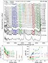 |
Fig. 7. Spectral evolution (upper) and line properties (lower) of the double-peaked type Ic SN 2013ge. The different spectral lines are denoted with the colors indicated in the upper panel. |
4.1.2. SN 2016coi
SN 2016coi is characterized by broad absorption lines such as SNe Ic-BL, but with He I features in the spectra (Prentice et al. 2018). The pEWs of He I lines seen in SN 2016coi are located at the lower end of SNe Ib. At approximately one week post-maximum light, the absorption feature near 5200 Å in the spectra of SN 2016coi exhibited a distinct double-Gaussian profile, as shown in Fig. 8. In contrast, typical Type Ib/c spectra show only a single Gaussian feature at this wavelength, which originates from either He I (Ib) or Na I (Ic) alone. Therefore, the corresponding line in SN 2016coi contains contributions from both elements. Furthermore, the He I lines at 6678 Å and 7065 Å can also be identified. Fig. 10 shows that the pEWs and velocity evolution of SN 2016coi lie well within the range of SNe Ic-BL. Consequently, SN 2016coi is established as an exemplary transitional object linking SNe Ib to SNe Ic-BL, which are characterized by a higher explosion energy while retaining a residual helium envelope (Yamanaka et al. 2017; Prentice et al. 2018; Terreran et al. 2019).
4.1.3. SN 2019ehk
SN 2019ehk is a calcium-rich supernova with double-peak light curves. The presentation of a full observation dataset from NIR to X-ray band and the analysis of its possible progenitor system were given by Jacobson-Galán et al. (2020). The very early spectrum of SN 2019ehk shows narrow emission lines of H I and He II, implying interaction with dense material surrounding the progenitor. The spectra of SN 2019ehk were characterized by strong Ca II absorption, prominent He I profiles and by the fast emergence of a [Ca II] profile a few days before maximum light. Although the He lines are present in the spectra, SN 2019ehk is classified as Ca-rich supernova. The progenitor system of SN 2019ehk remains debated. Jacobson-Galán et al. (2020) proposed a low-mass binary white dwarf for the origin of SN 2019ehk based on its explosion and environment properties, while other studies proposed alternative scenarios involving the collapse of stripped massive stars for these Ca-rich envents (De et al. 2021; Nakaoka et al. 2021; Ertini et al. 2023).
Compared with SNe Ib, SN 2019ehk has very weak absorption lines before 10 days since maximum light. This time coincidence with the first light-curve peak can be attributed to interaction with a dense circumstellar matter shell (Jacobson-Galán et al. 2020). The high temperature of the ejecta blocks any information from spectral features, producing nearly featureless spectra.
4.2. Hydrogen lines in SNe Ib and IIb
In SNe Ib and Ic, the blended line feature in the wavelength range of 6000–6400 Å can be attributed to several different ions. In early-phase SNe Ib spectra, potential contributors include Fe II, Ca I, Si II, and possibly H I, with an additional contribution from He I that strengthens over time (Dessart et al. 2012), while in SNe Ic, the He Iλ6678 line is replaced by the C IIλ6580 line, which fades gradually. Previous studies have identified H features in most SNe Ib, suggesting a continuous spectroscopic sequence between types IIb and Ib (Liu et al. 2016; Holmbo et al. 2023). A possible contribution of Si II to the spectra of SNe Ib was also discussed by Holmbo et al. (2023). In this section, we focus on the evolutionary properties of H features in SN Ib spectra and compare their similarities and differences with those of SNe IIb.
In SN Ib spectra at phases earlier than +10 days, the absorption feature near 6200 Å can be attributed to Hα, Si IIλ6355, or a blend of the two. Prior to maximum light, all SN Ib spectra in our sample exhibit an absorption feature near 6200 Å. The top panel of Fig. 9 shows early-time spectra of SNe Ib, covering the wavelength range of 5000–7000 Å. The spectral profiles between 6000 and 6500 Å are generally consistent across different objects, although variations in absorption depth and velocity are observed. Holmbo et al. (2023) attributed the blue part of this feature (the blue wing) in SNe Ib to high-velocity Si IIλ6355 and the red part (the red wing) to Hα. These two components, combined with the He Iλ6678 line, form a triplet line structure. When inspecting this feature, we noted that the triplet feature is absent in all early-phase (i.e., t ≲ +10 d) spectra (Fig. 9, upper panel). If the blue wing is attributed to Si IIλ6355, its measured blueshift velocity is significantly higher than that of the Fe IIλ5169 in the same spectrum. However, our measurements of SN Ic spectra show that Si II velocities are typically slightly lower than those of the Fe II lines (Fig. 10(c)). Furthermore, after +10 days, the blue-wing component strengthens and emerges concurrently with an absorption structure near 5350 Å, which is marked by green shading in the upper panel of Fig. 9. This feature near 5350 Å might be Sc II/Fe IIλ5531, and thus, this blue-wing feature might also originate from Sc II/Fe II. Considering this consistent evidence (the atypical velocity, the late emergence, and the association with the 5350 Å line), we conclude that the blue-wing absorption is unlikely to be Si II.
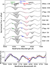 |
Fig. 9. Upper: Normalized spectra of SNe Ib in our sample till maximum light in the range of 5000–7000 Å, showing the features around Hα. The spectra of different SNe are plotted in distinct colors and shifted vertically for better illustration. The main absorption features are highlighted with distinct colored shaded areas. The green bands in the areas denote an absorption line of ambiguous origin that appears concurrently with the blue-wing structure. Lower: Normalized spectrum of SN 2015ah at −8-d showing the range of the doublet feature near 6200 Å. Synthetic spectra by SYNOW with either HI (solid red line) or Si II (dashed blue line) are also overplotted. |
The absorption feature on the red wing might originate from either H I or Si II. Liu et al. (2016) identified it as Hα and found that its pEWs and velocity evolution differed significantly from those of SNe IIb, without ruling out a possible Si II contribution. In contrast, Holmbo et al. (2023) attributed the aforementioned blue wing to Si II and the red wing to Hα, finding no substantial difference in the Hα line velocities between SNe IIb and Ib. Our SYNOW spectral synthesis (Fig. 9, lower panel) also shows that the asymmetric and broad-line profile can be better synthesized with an H I component. In the model including H I, the H I velocity is higher than that of other ions by about 7000 km s−1. While definitive confirmation of the carrier (Si II or H I) from a single spectrum is challenging, the dominant role of H I is supported by our fitting. To further investigate this, we next performed a statistical analysis of the properties of this feature under both assumptions.
First, we considered the line as Si IIλ6355. The line velocities and pEWs of Si IIλ6355 alongside those of Fe II is presented in Fig. 10. For comparison, measurements for SNe Ic and Ic-BL are included in the same figure. To enable a more meaningful comparison of the subtypes, we supplemented the spectral dataset from WISeREP or the literature of several SNe Ib in our sample that exhibit the distinct red-wing feature (as shown in Fig. 9) and also lack early-time spectroscopic data. Accordingly, we retrieved and uniformly processed publicly available data for the following SNe: iPTF13bvn (Cao et al. 2013; Srivastav et al. 2014; Childress et al. 2016), 2015ah (Shivvers et al. 2019; Prentice et al. 2019), 2019yvr, 2020hvp (Yesmin et al. 2025), and 2020zgl. These additional measurements are plotted as open symbols in Fig. 10. Notably, the inclusion of these objects, particularly iPTF13bvn, extends the observed parameter space for SNe Ib, which is representative of objects with relatively strong red-wing features. In terms of velocity, the three subtypes follow a similar correlation, while SNe Ib and Ic are similar and SNe Ic-BL are the fastest, which is consistent with previous studies (e.g., Liu et al. 2016; Holmbo et al. 2023). However, the pEWs of this line in SNe Ib are larger than those in SNe Ic and Ic-BL, especially in early phases, while the latter two types are not distinguishable. This implies that the origin of the red-wing feature in SNe Ib is different from that in SNe Ic and Ic-BL. Thus, we conclude that the red-wing feature in spectra of SNe Ib is very likely due to H I and not to Si II. Given the symmetric Gaussian profile of the red-wing feature, any contribution from Si II to this feature would be negligible.
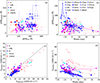 |
Fig. 10. Pseudo-equivalent widths and velocities of the red-wing feature (attributed to Si IIλ6355) and Fe II lines in the spectra of SNe Ib compared with SNe Ic and Ic-BL. Different subtypes are color-coded, including the peculiar objects SN 2016coi and SN 2019ehk. The data points belonging to the same SN are connected by lines, and those measured from WiseRep spectra are shown with empty symbols. Each SN Ib is represented by a distinct symbol denoted in the legend of (b). |
On the other hand, if the absorption feature is attributed to Hα, the comparison between SNe Ib and IIb is presented Fig. 11. We also incorporated supplementary spectral data from the literature for the SNe IIb in our sample, including 2011dh (Arcavi et al. 2011; Ergon et al. 2014; Shivvers et al. 2019), 2011fu (Kumar et al. 2013; Morales-Garoffolo et al. 2015; Shivvers et al. 2019), 2014ds (Shivvers et al. 2019), 2015bi (Shivvers et al. 2019), and 2017gpn (Prentice et al. 2019). It shows that the two subtypes exhibit distinct distributions at early phases (< +10 days): most SNe Ib show a weaker Hα line, but stronger Fe II lines. In early phases, the two subtypes occupy opposite extremes of this population with little overlap: SNe IIb display lower Hα velocities, but greater line strengths, consistent with Liu et al. (2016). Although several SNe Ib (e.g., the most H-rich iPTF13bvn) have strong Hα lines at very early epochs (t < –10 d), their pEWs decline rapidly approaching maximum light. In iPTF13bvn, the early strong Hα is accompanied by notably strong Fe II lines, further distinguishing it from SNe IIb. After +10 days post maximum, the Hα line strengths in SNe IIb fade. Consequently, their locus in the Hα-Fe II line-strength relation shifts toward the region occupied by SNe Ib, resulting in a weaker distinction between the two subtypes. For objects displaying He I and prominent Hα lines, the Fe II line strength can aid in distinguishing between types IIb and Ib. However, an accurate classification may not be possible for SNe with very weak Hα lines based on spectral line strengths alone.
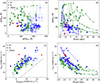 |
Fig. 11. Same as Fig. 10, but the red-wing feature attributed to Hα in the spectra of SNe Ib and compared with SNe IIb. The data points circled in (a) correspond to phases later than +10 days. See the main text for details. |
In terms of the line velocity, the Hα and Fe II velocity distributions of SNe IIb largely overlap with the slower portion of the SNe Ib distributions. Moreover, the Hα line velocities in SNe Ib decline to a level comparable to those in SNe IIb within 10 days after maximum light (Fig. 11(d)). This implies that the hydrogen shell present in SNe Ib may be thinner than that in SNe IIb. Our findings are consistent with those of Liu et al. (2016).
To conclude, the absorption feature near 6200 Å can conclusively be identified as Hα. However, it should be noted that the dataset of SNe IIb is quite small, which increases the uncertainty of our conclusion.
4.3. Evolution and correlation of the line velocities
Fig. A.2 shows the temporal evolution of the expansion velocities of all lines present in each subclass. In general, the expansion velocities of all lines decline over time. SNe Ic-BL exhibit distinctly higher velocities than the other subclasses. SNe Ic show higher average velocities than SNe Ib, although their distributions overlap considerably. Finally, SNe IIb have the lowest velocities. This trend of increasing velocities among SNe IIb to Ic and Ic-BL is not new, but was previously reported by Liu et al. (2016), Modjaz et al. (2016). These differences are caused by either distinction in the distribution of explosion energy or ejecta mass. Given that SNe Ic-BL are found to have the highest ejecta masses of all subtypes, as inferred from light-curve analyses (e.g., Prentice et al. 2019), their exceptionally high velocities must originate from intrinsically greater explosion energies. This points to a different explosion mechanism or energy source (e.g., a central engine). For the other three subtypes, the velocity differences are subtler, and their ejecta mass distributions are similar according to the literature. Therefore, the progressive velocity increase from type IIb to type Ic, which corresponds to more extensive envelope stripping, might arise from relatively smaller differences in explosion energy. This energy difference might be linked to the stripping process itself, for instance, faster rotation of the progenitor or more intense binary interaction might result in a higher explosion energy (Schneider et al. 2021), or additional energy input similar to that proposed for SNe Ic-BL. Numerous other factors, such as the excitation state of the materials and the degree of elemental mixing, might also contribute to variations in the spectral line velocities. These aspects, however, are beyond the scope of this study.
Ions are distributed across different layers within the SNe ejecta, resulting in differences in expansion velocity, temperature, density, and other properties of their respective spectral line-forming regions. Typically, lighter elements are located in outer layers, and thus, exhibit higher velocities under the assumption of homologous expansion. The difference in velocity between elements in adjacent layers is generally smaller.
To quantify the correlations between different spectral line measurements, we used Spearman’s rank correlation coefficient ρ. The absolute value of ρ indicates the strength of the correlation, and its sign indicates a positive (ρ > 0) or negative (ρ < 0) relation. The larger ρ, the stronger the correlation between the corresponding pair of measurements, i.e., weak (0.4 < |ρ| ≤ 0.6), moderate (0.6 < |ρ| ≤ 0.8), and strong (|ρ| > 0.8) correlation. The exact p-value for each correlation test is available at the CDS.
We examined the correlations between the expansion velocities of the various spectral lines of each subtype. The raw data of the line velocity correlation are presented in Fig. A.4, and the correlation matrices are shown in Fig. 12. The ions in Fig. 12 are arranged such that lighter elements are positioned toward the right and top to reflect the expected stratification in the ejecta. All spectral lines are included to facilitate the comparison across subtypes.
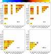 |
Fig. 12. Spearman’s rank correlation coefficients (ρ) between the measured velocities of lines of different types of SESNe. The ions are arranged such that lighter elements are positioned toward the right and top. The numbers in each box show the coefficients of the corresponding line pairs. Boxes in gray show low statistical significance with a p value higher than 0.05. These cases are all due to the very small dataset. The numeric values are indicated by the color bar at the top of the figure, with lighter colors indicating stronger correlation. Data behind the figure are available at the CDS. |
The spectral line velocities across all subtypes exhibit positive correlations of varying strength, in agreement with the expectation of homologously expanding ejecta. Figure 12 shows that the correlation between the Fe II lines and the other lines progressively strengthens from type IIb to type Ic/Ic-BL. In SNe IIb and Ib, the He I line velocities exhibit a weaker correlation with those of heavier elements, whereas Hα velocities show a stronger correlation with metal lines. The generally weaker correlations in SNe IIb might be attributable to their smaller sample size. The velocity distributions of nearly all common spectral lines overlap across subtypes and follow similar correlation patterns. A notable exception is the Hα–O Iλ7774 pair, for which SNe Ib show systematically higher Hα velocities than SNe IIb. Although the helium shell is situated in the outer ejecta, our measurements show that He I line velocities are not consistently higher than those of Fe II lines. For example, the velocity of He Iλ7065 shows virtually no correlation with Fe IIλ5169 (except for a few high-velocity outliers), and He Iλ6678 is generally slower than Fe IIλ5169. Of the four He I lines we studied, He Iλ7281 exhibits the highest velocities, but approximately half of its measurements still fall below those of Fe IIλ5169.
By examining the spectral lines common to all four subtypes (namely Fe II, O I, and Ca II), we found the following. First, the Ca II lines exhibit the highest expansion velocities. Second, SNe Ib are more prevalent at the lower-velocity end of the distributions. Third, the velocity correlations in SNe Ic are stronger than in the other subtypes, indicating a lower dispersion in their velocities. When we compared SNe Ic and SNe Ic-BL, in addition to exhibiting generally lower velocities in SNe Ic, they differed in their relation between the velocities of the Na I D and Si IIλ6355 lines: SNe Ic show lower velocities for the Na I D line. The distributions for other spectral lines are similar for these two subtypes.
4.4. Evolution and correlation of the line intensities
The temporal evolution of line intensities (pEWs) of the four subtypes SNe is shown in Fig. A.3. The spectral lines of residual elements (i.e., H in SNe Ib and C in SNe Ic/Ic-BL) weaken over time and become undetectable around 10 days after the maximum light. Although the Si lines in SNe Ic/Ic-BL eventually vanish as well, they undergo a short period of slight strengthening before fading.
In early phases (t < −10 d), the Hα line in SNe IIb exhibits pEWs comparable to those in SNe Ib. However, in SNe IIb, the Hα strength continues to increase until after maximum light, after which it weakens, although the onset of the weakening varies among objects. In SNe Ib, the intensities of most He I lines generally decline after maximum. An exception is the He Iλ7281 line, which shows no clear weakening in our sample. This might be due to contamination from the gradually emerging [Ca II] emission line near 7300 Å in later phases, which might distort the pEW measurement of the He Iλ7281 feature. The intensities of the He Iλ5876 and He Iλ6678 lines are significantly stronger in SNe Ib, consistent with results from Liu et al. (2016). However, the two subtypes exhibit no difference in the intensity evolution of the He Iλ7281 line, consistent with Holmbo et al. (2023). For the He Iλ7065 line, our data show that its strength in SNe IIb exceeds that in SNe Ib at later phases. This finding is consistent with Liu et al. (2016), but contrasts with Fremling et al. (2018) and Holmbo et al. (2023).
Among the subtypes, O I lines are strongest in SNe Ic/Ic-BL, intermediate in SNe Ib, and weakest in SNe IIb. The intensity of the O Iλ7774 line in SNe Ic covers the upper range of the distribution observed in SNe Ib, and there is no significant difference in the intensity distribution of this line between the broad-lined and normal SNe Ic. Ca II and Fe II lines are weakest in SNe IIb, while no statistically significant differences are observed among the other three subtypes.
Fig. A.3 shows the correlation of line intensities of the four subclasses of SESNe, and the Spearman’s rank correlation coefficients between the pEWs of lines are shown in Fig. 13. Regarding light elements (H and He), as discussed in Sect. 4.2, SNe IIb and SNe Ib are distinguishable in the Hα-Fe II space, where SNe IIb are characterized by stronger Hα and weaker Fe II lines. The pEWs of He Iλ7065 line shows weak correlations with those of the He Iλ5876, He Iλ7065, and the Ca II NIR lines. Compared with SNe Ib, the intensities of He I lines are more strongly correlated with that of O I line in SNe IIb. For SNe Ic and Ic-BL, no correlation is found between the pEWs of the C II/O I lines and those of other lines. The pEWs of the Na I and Ca II lines exhibit strong/moderate correlations in SNe Ic/Ic-BL spectra. However, the correlation between the pEWs of Na I and Fe II is relatively weaker in SN Ic spectra, while that between Na I and Si II is stronger. The distributions of the pEW relation between Fe II and Ca II of the four subtypes appear to belong to a single population. Nevertheless, the correlation appears to be strongest in SNe Ic, followed by SNe Ic-BL.
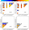 |
Fig. 13. Same as in Fig. 12, but for measurements of pEWs of each line. Data behind the figure are available at the CDS. |
4.5. Nebular-phase spectra
Nebular-phase spectra are available for a limited number of SNe in our sample. To ensure a complete transition to the nebular phase, we only included spectra observed at phases > 90 days post maximum in this analysis. The nebular-phase spectra of each subtype are shown in Fig. 14. In SN 2014C, the narrow emission near 6560 Å is Hα formed by interaction with the circumstellar medium (Mauerhan et al. 2018; Zhai et al. 2025). The most dominant emission lines common to all subtypes of SESNe are O Iλ7774, [O I]λλ6300,6364, the Ca II NIR triplet, [Ca II]λλ7291,7324, and Na I D. Notably, the Mg I]λ4571 line is rather weak in SNe IIb and Ib. The luminosities of [O I]λλ6300,6364 and [Ca II]λλ7291,7323 are related to the CO core mass, and hence, to the initial mass of the progenitor stars. We measured L[OI], L[NII] and L[CaII] following the method described in Fang et al. (2019) and Fang et al. (2022). In Fig. 15 we show the distribution of L[NII]/L[OI] and L[OI]/L[CaII]. The measurements from Fang et al. (2019) are also plotted as empty symbols for comparison. Fig. 14 shows that the line strength ratio of [O I] to [Ca II] in SNe IIb/Ib is markedly lower than that in SNe Ic, suggesting that SNe Ic have more massive progenitors. SN 2014C exhibits the highest L[OI], L[NII] in the whole dataset, probably due to the additional hydrogen emission from late-time interaction with hydrogen-rich circumstellar material. Although the presence of He was spectroscopically confirmed in the photospheric phase spectra of SN 2016coi, its nebular-phase spectrum closely resembles that of a typical SN Ic or SN Ic-BL, exhibiting remarkably stronger [O I] emission than [Ca II].
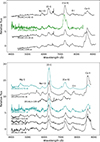 |
Fig. 14. Top: Nebular spectra of SNe Ib (black) and one type IIb (green). Bottom: Nebular spectra of SNe Ic (black), and the peculiar He-rich broad-lined SN 2016coi (cyan). The SN names and the corresponding phases are displayed below each spectrum. |
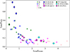 |
Fig. 15. Distribution of L[NII]/L[OI] and L[OI]/L[CaII] measured from the nebular-phase spectra of our sample. The data from literature are plotted as empty symbols (Fang et al. 2019). |
5. Summary
We presented the spectrum dataset of stripped-envelope supernovae (SESNe) collected by the Tsinghua University-Yunnan Observatory supernova group. Observations were conducted from 2010 to 2020 using the 2.16 m telescope at Beijing Xinglong Observatory and the 2.4 m telescope at Lijiang Observatory. The dataset contains 249 spectra for 62 SESNe, including 20 spectra of 12 SNe IIb, 76 spectra of 20 SNe Ib, 85 spectra of 19 SNe Ic, and 68 spectra of 11 SNe Ic-BL. The SNe in our sample have an average redshift of 0.015, with the farthest one at z = 0.06. The phases of the dataset cover a range from –16 to over 190 days since the maximum light.
For each SN, we performed a detailed spectroscopic classification to resolve discrepancies or misclassifications in public databases. The time of maximum light was determined using our follow-up photometric observations or published photometric data. For SNe lacking reliable light curves, the epoch of each spectrum was estimated via spectral cross correlation using SNID.
For each spectrum, we identified the dominant spectral lines according to previous empirical identification results, and we measured the pseudo-equivalent widths (pEWs) and blueshift velocities of each line. A key focus was the absorption feature near 6200 Å in early-phase (≲+10 days) SNe Ib spectra, which has been subject to divergent interpretations in the literature. We analyzed this feature by comparing SNe Ib to SNe IIb and Ic, testing Hα and Si IIλ6355 identifications. Our results show that its properties in SNe Ib agree more closely with Hα in SNe IIb, and we therefore identify it as Hα. This indicates that residual hydrogen is common in SNe Ib, with some early spectra showing Hα strengths comparable to those in SNe IIb. This supports a continuous stripping sequence from type IIb to Ib progenitors. The main spectroscopic differences are that in SNe IIb, Hα continues to strengthen after maximum light, whereas in SNe Ib, it weakens rapidly before maximum. Additionally, Hα velocities are systematically higher in SNe Ib.
Expanding on the analytical method employed in prior studies of SESNe spectral samples (Liu et al. 2016; Fremling et al. 2018; Holmbo et al. 2023), we examined the correlations in velocity and strength among the common spectral features shared by the four subtypes. The velocities of nearly all common spectral lines exhibit overlapping distributions across different subtypes and follow similar correlation patterns, suggesting that they represent variations within a continuous population. An exception is the Hα-O Iλ7774 pair between type IIb and type Ib, where SNe Ib show systematically higher Hα velocities than SNe IIb, marking a distinct deviation from the trend defined by the latter. A velocity gradient is observed across subtypes of SESNe, with SNe Ic exhibiting the highest line velocities, followed by normal SNe Ic, SNe Ib, and SNe IIb, consistent with prior statistical studies. In SNe Ic and Ic-BL, the velocities of different ions are more tightly correlated than in SNe IIb and Ib, implying more compact progenitor cores in the He-poor subtypes. Furthermore, the distribution of the Fe II line strength inferred for SNe Ib agrees more closely with that of SNe Ic/Ic-BL, which is systematically stronger than in SNe IIb.
In the correlation between the spectral line intensities (pEWs), SNe IIb and Ib are most clearly distinguished by their early-phase (≲+10 d) Hα-Fe II relation: SNe IIb exhibit stronger Hα lines alongside weaker Fe II lines. However, at later epochs, as the strength of Hα lines in SNe IIb declines to levels comparable to those in SNe Ib, the two subclasses become indistinguishable in the Hα-Fe II diagnostic diagram. At this stage, distinguishing between them may require additional spectral diagnostics, such as the strength of He I lines. In addition, He I line intensities are more strongly correlated with that of O I line in SNe IIb than in SNe Ib. The oxygen lines in SNe IIb/Ib are weaker than in SNe Ic/Ic-BL. The distributions of the spectral line intensities show no significant differences between type Ic and type Ic-BL.
Our dataset includes 11 nebular-phase spectra. In the spectra of SNe IIb/Ib, [Ca II] emission dominates [O I], whereas SNe Ic, including the helium-rich broad-lined SN 2016coi, display stronger [O I] lines. We measured the luminosities of the [O I], [N II], and [Ca II] lines and calculated their ratios. SNe Ic exhibit significantly higher [O I]/[Ca II] luminosity ratios than SNe IIb/Ib, suggesting that their progenitors had more massive CO cores and, consequently, higher initial masses.
The spectroscopic data presented here expand the sample of SESNe, providing additional material for future studies on the distinctions, connections, and progenitor properties of these supernovae. The analytical method we adopted, which incorporates strengths from multiple existing approaches, can serve as a reference for more in-depth statistical studies when a more comprehensive spectroscopic database is established in the future.
Data availability
All spectral data used in this work are available via the WiseREP (https://www.wiserep.org/). Full Table A.2 and data behind Figs. 12, 13 are available at the CDS via https://cdsarc.cds.unistra.fr/viz-bin/cat/J/A+A/708/A267
Acknowledgments
We acknowledge the support of the staff of the Lijiang 2.4-m and Xinglong 2.16-m telescopes. This work is supported by the National Natural Science Foundation of China (NSFC, grants 12288102 and 12033003), and the Tencent Xplorer Prize. DFX is supported by the National Natural Science Foundation of China (grant 12503047). JZ is supported by the B-type Strategic Priority Program of the Chinese Academy of Sciences (Grant No. XDB1160202), the National Key R&D Program of China with grant 2021YFA1600404, the National Natural Science Foundation of China (NSFC grants 12173082 and 12333008), the Yunnan Fundamental Research Projects (YFRP; grants 202501AV070012 and 202401BC070007), the Top-notch Young Talents Program of Yunnan Province, the Light of West China Program provided by the Chinese Academy of Sciences, and the International Centre of Supernovae, Yunnan Key Laboratory (grant 202302AN360001). Funding for the LJT has been provided by the CAS and the People’s Government of Yunnan Province. The LJT is jointly operated and administrated by YNAO and Center for Astronomical Mega-Science, CAS. H.L. was supported by the National Natural Science Foundation of China (NSFC grants No. 12403061) and the innovative project of ‘Caiyun Postdoctoral Project’ of Yunnan Province. Y.-Z. Cai is supported by the National Natural Science Foundation of China (NSFC, Grant No. 12303054), the National Key Research and Development Program of China (Grant No. 2024YFA1611603), and the Yunnan Fundamental Research Projects (Grant Nos. 202401AU070063, 202501AS070078). Chengyuan Wu is supported by the National Natural Science Foundation of China (No. 12473032), the Yunnan Revitalization Talent Support Program-Young Talent project, and the Yunnan Fundamental Research Project (No. 202501AW070001). JNF acknowledges the support from the National Natural Science Foundation of China (NSFC) through the grants 12090040, 12090042 and 12427804. This work is partly supported by the China Manned Space Program with grant no. CMS-CSST-2025-A13, the Tianchi Talent Introduction Plan, and the Central Guidance for Local Science and Technology Development Fund under No. ZYYD2025QY27.
References
- Arcavi, I., Gal-Yam, A., Yaron, O., et al. 2011, ApJ, 742, L18 [Google Scholar]
- Balakina, E. A., Pruzhinskaya, M. V., Moskvitin, A. S., et al. 2021, MNRAS, 501, 5797 [NASA ADS] [CrossRef] [Google Scholar]
- Banerjee, D. P. K., Joshi, V., Evans, A., et al. 2018, MNRAS, 481, 806 [CrossRef] [Google Scholar]
- Bellm, E. C., Kulkarni, S. R., Graham, M. J., et al. 2019, PASP, 131, 018002 [Google Scholar]
- Bersten, M. C., Benvenuto, O. G., Folatelli, G., et al. 2014, AJ, 148, 68 [NASA ADS] [CrossRef] [Google Scholar]
- Blondin, S., & Tonry, J. L. 2007, ApJ, 666, 1024 [NASA ADS] [CrossRef] [Google Scholar]
- Brown, P. J., Breeveld, A. A., Holland, S., Kuin, P., & Pritchard, T. 2014, Ap&SS, 354, 89 [Google Scholar]
- Cao, Y., Kasliwal, M. M., Arcavi, I., et al. 2013, ApJ, 775, L7 [NASA ADS] [CrossRef] [Google Scholar]
- Childress, M. J., Tucker, B. E., Yuan, F., et al. 2016, PASA, 33, e055 [NASA ADS] [CrossRef] [Google Scholar]
- Das, K. K., Fremling, C., Kasliwal, M. M., et al. 2024, ApJ, 969, L11 [NASA ADS] [CrossRef] [Google Scholar]
- De, K., Fremling, U. C., Gal-Yam, A., et al. 2021, ApJ, 907, L18 [NASA ADS] [CrossRef] [Google Scholar]
- D’Elia, V., Campana, S., D’Aì, A., et al. 2018, A&A, 619, A66 [NASA ADS] [CrossRef] [EDP Sciences] [Google Scholar]
- Dessart, L., Hillier, D. J., Li, C., & Woosley, S. 2012, MNRAS, 424, 2139 [NASA ADS] [CrossRef] [Google Scholar]
- Dessart, L., Hillier, D. J., Sukhbold, T., Woosley, S. E., & Janka, H.-T. 2021, A&A, 656, A61 [NASA ADS] [CrossRef] [EDP Sciences] [Google Scholar]
- Drout, M. R., Milisavljevic, D., Parrent, J., et al. 2016, ApJ, 821, 57 [NASA ADS] [CrossRef] [Google Scholar]
- Eldridge, J. J., & Maund, J. R. 2016, MNRAS, 461, L117 [NASA ADS] [CrossRef] [Google Scholar]
- Eldridge, J. J., Fraser, M., Maund, J. R., & Smartt, S. J. 2015, MNRAS, 446, 2689 [CrossRef] [Google Scholar]
- Ergon, M., Sollerman, J., Fraser, M., et al. 2014, A&A, 562, A17 [NASA ADS] [CrossRef] [EDP Sciences] [Google Scholar]
- Ertini, K., Folatelli, G., Martinez, L., et al. 2023, MNRAS, 526, 279 [NASA ADS] [CrossRef] [Google Scholar]
- Fan, Y.-F., Bai, J.-M., Zhang, J.-J., et al. 2015, RAA, 15, 918 [Google Scholar]
- Fan, Z., Wang, H., Jiang, X., et al. 2016, PASP, 128, 115005 [NASA ADS] [CrossRef] [Google Scholar]
- Fang, Q., & Maeda, K. 2023, ApJ, 949, 93 [Google Scholar]
- Fang, Q., Maeda, K., Kuncarayakti, H., Sun, F., & Gal-Yam, A. 2019, Nat. Astron., 3, 434 [Google Scholar]
- Fang, Q., Maeda, K., Kuncarayakti, H., et al. 2022, ApJ, 928, 151 [NASA ADS] [CrossRef] [Google Scholar]
- Filippenko, A. V. 1997, ARA&A, 35, 309 [NASA ADS] [CrossRef] [Google Scholar]
- Fox, O. D., Van Dyk, S. D., Williams, B. F., et al. 2022, ApJ, 929, L15 [NASA ADS] [CrossRef] [Google Scholar]
- Fremling, C., Sollerman, J., Taddia, F., et al. 2016, A&A, 593, A68 [NASA ADS] [CrossRef] [EDP Sciences] [Google Scholar]
- Fremling, C., Sollerman, J., Kasliwal, M. M., et al. 2018, A&A, 618, A37 [NASA ADS] [CrossRef] [EDP Sciences] [Google Scholar]
- Frey, L. H., Fryer, C. L., & Young, P. A. 2013, ApJ, 773, L7 [Google Scholar]
- Gal-Yam, A. 2017, in Handbook of Supernovae, eds. A. W. Alsabti, & P. Murdin (Springer), 195 [Google Scholar]
- Gal-Yam, A., Bruch, R., Schulze, S., et al. 2022, Nature, 601, 201 [NASA ADS] [CrossRef] [Google Scholar]
- Gangopadhyay, A., Misra, K., Sahu, D. K., et al. 2020, MNRAS, 497, 3770 [Google Scholar]
- Gomez, S., Berger, E., Nicholl, M., Blanchard, P. K., & Hosseinzadeh, G. 2022, ApJ, 941, 107 [NASA ADS] [CrossRef] [Google Scholar]
- Grayling, M., Gutiérrez, C. P., Sullivan, M., et al. 2021, MNRAS, 505, 3950 [Google Scholar]
- Ho, A. Y. Q., Goldstein, D. A., Schulze, S., et al. 2019, ApJ, 887, 169 [Google Scholar]
- Holmbo, S., Stritzinger, M. D., Karamehmetoglu, E., et al. 2023, A&A, 675, A83 [NASA ADS] [CrossRef] [EDP Sciences] [Google Scholar]
- Huang, F., Li, J.-Z., Wang, X.-F., et al. 2012, RAA, 12, 1585 [Google Scholar]
- Jacobson-Galán, W. V., Margutti, R., Kilpatrick, C. D., et al. 2020, ApJ, 898, 166 [CrossRef] [Google Scholar]
- Jerkstrand, A., Smartt, S. J., Fraser, M., et al. 2014, MNRAS, 439, 3694 [Google Scholar]
- Jerkstrand, A., Ergon, M., Smartt, S. J., et al. 2015, A&A, 573, A12 [NASA ADS] [CrossRef] [EDP Sciences] [Google Scholar]
- Jordi, K., Grebel, E. K., & Ammon, K. 2006, A&A, 460, 339 [NASA ADS] [CrossRef] [EDP Sciences] [Google Scholar]
- Kilpatrick, C. D., Drout, M. R., Auchettl, K., et al. 2021, MNRAS, 504, 2073 [CrossRef] [Google Scholar]
- Kumar, B., Pandey, S. B., Sahu, D. K., et al. 2013, MNRAS, 431, 308 [NASA ADS] [CrossRef] [Google Scholar]
- Kuncarayakti, H., Maeda, K., Bersten, M. C., et al. 2015, A&A, 579, A95 [CrossRef] [EDP Sciences] [Google Scholar]
- Kuncarayakti, H., Maeda, K., Dessart, L., et al. 2022, ApJ, 941, L32 [NASA ADS] [CrossRef] [Google Scholar]
- Li, W., Wang, X., Bulla, M., et al. 2021, ApJ, 906, 99 [Google Scholar]
- Lin, H., Wang, X., Zhang, J., et al. 2024, MNRAS, 528, 3092 [Google Scholar]
- Liu, Z., Zhao, X.-L., Huang, F., et al. 2015, RAA, 15, 225 [Google Scholar]
- Liu, Y.-Q., Modjaz, M., Bianco, F. B., & Graur, O. 2016, ApJ, 827, 90 [NASA ADS] [CrossRef] [Google Scholar]
- Ma, X., Wang, X., Mo, J., et al. 2025a, A&A, 698, A306 [NASA ADS] [CrossRef] [EDP Sciences] [Google Scholar]
- Ma, X., Wang, X., Mo, J., et al. 2025b, A&A, 698, A305 [NASA ADS] [CrossRef] [EDP Sciences] [Google Scholar]
- Masci, F. J., Laher, R. R., Rusholme, B., et al. 2019, PASP, 131, 018003 [Google Scholar]
- Mauerhan, J. C., Filippenko, A. V., Zheng, W., et al. 2018, MNRAS, 478, 5050 [NASA ADS] [CrossRef] [Google Scholar]
- Milisavljevic, D., Patnaude, D. J., Raymond, J. C., et al. 2017, ApJ, 846, 50 [Google Scholar]
- Modjaz, M., Blondin, S., Kirshner, R. P., et al. 2014, AJ, 147, 99 [Google Scholar]
- Modjaz, M., Liu, Y. Q., Bianco, F. B., & Graur, O. 2016, ApJ, 832, 108 [NASA ADS] [CrossRef] [Google Scholar]
- Morales-Garoffolo, A., Elias-Rosa, N., Bersten, M., et al. 2015, MNRAS, 454, 95 [CrossRef] [Google Scholar]
- Nagao, T., Kuncarayakti, H., Maeda, K., et al. 2023, A&A, 673, A27 [NASA ADS] [CrossRef] [EDP Sciences] [Google Scholar]
- Nakaoka, T., Maeda, K., Yamanaka, M., et al. 2021, ApJ, 912, 30 [NASA ADS] [CrossRef] [Google Scholar]
- Pellegrino, C., Howell, D. A., Terreran, G., et al. 2022, ApJ, 938, 73 [NASA ADS] [CrossRef] [Google Scholar]
- Podsiadlowski, P. 1992, PASP, 104, 717 [CrossRef] [Google Scholar]
- Prentice, S. J., Ashall, C., Mazzali, P. A., et al. 2018, MNRAS, 478, 4162 [NASA ADS] [CrossRef] [Google Scholar]
- Prentice, S. J., Ashall, C., James, P. A., et al. 2019, MNRAS, 485, 1559 [NASA ADS] [CrossRef] [Google Scholar]
- Pritchard, T. A., Bensch, K., Modjaz, M., et al. 2021, ApJ, 915, 121 [Google Scholar]
- Rho, J., Evans, A., Geballe, T. R., et al. 2021, ApJ, 908, 232 [NASA ADS] [CrossRef] [Google Scholar]
- Richardson, D., Jenkins, R. L., III, Wright, J., & Maddox, L. 2014, AJ, 147, 118 [NASA ADS] [CrossRef] [Google Scholar]
- Sahu, D. K., Anupama, G. C., Chakradhari, N. K., et al. 2018, MNRAS, 475, 2591 [NASA ADS] [CrossRef] [Google Scholar]
- Sana, H., de Mink, S. E., de Koter, A., et al. 2012, Science, 337, 444 [Google Scholar]
- Schlafly, E. F., & Finkbeiner, D. P. 2011, ApJ, 737, 103 [Google Scholar]
- Schneider, F. R. N., Podsiadlowski, P., & Müller, B. 2021, A&A, 645, A5 [NASA ADS] [CrossRef] [EDP Sciences] [Google Scholar]
- Schulze, S., Gal-Yam, A., Dessart, L., et al. 2025, Nature, 644, 634 [Google Scholar]
- Shahbandeh, M., Hsiao, E. Y., Ashall, C., et al. 2022, ApJ, 925, 175 [NASA ADS] [CrossRef] [Google Scholar]
- Shivvers, I., Filippenko, A. V., Silverman, J. M., et al. 2019, MNRAS, 482, 1545 [Google Scholar]
- Srivastav, S., Anupama, G. C., & Sahu, D. K. 2014, MNRAS, 445, 1932 [NASA ADS] [CrossRef] [Google Scholar]
- Stritzinger, M., Hsiao, E. Y., Morrell, N., et al. 2016, TNS Classif. Rep., 2016-1117, 1 [Google Scholar]
- Stritzinger, M. D., Taddia, F., Lawrence, S. S., et al. 2022, ApJ, 939, L8 [CrossRef] [Google Scholar]
- Stritzinger, M. D., Holmbo, S., Morrell, N., et al. 2023, A&A, 675, A82 [NASA ADS] [CrossRef] [EDP Sciences] [Google Scholar]
- Stritzinger, M. D., Baron, E., Taddia, F., et al. 2024, A&A, 686, A79 [NASA ADS] [CrossRef] [EDP Sciences] [Google Scholar]
- Sun, N.-C., Maund, J. R., Crowther, P. A., et al. 2022, MNRAS, 510, 3701 [NASA ADS] [CrossRef] [Google Scholar]
- Takaki, K., Kawabata, K. S., Yamanaka, M., et al. 2013, ApJ, 772, L17 [NASA ADS] [CrossRef] [Google Scholar]
- Tauris, T. M., Langer, N., & Podsiadlowski, P. 2015, MNRAS, 451, 2123 [NASA ADS] [CrossRef] [Google Scholar]
- Terreran, G., Margutti, R., Bersier, D., et al. 2019, ApJ, 883, 147 [NASA ADS] [CrossRef] [Google Scholar]
- Thomas, R. C., Nugent, P. E., & Meza, J. C. 2011, PASP, 123, 237 [NASA ADS] [CrossRef] [Google Scholar]
- Tody, D. 1986, SPIE Conf. Ser., 627, 733 [Google Scholar]
- Tody, D. 1993, ASP Conf. Ser., 52, 173 [NASA ADS] [Google Scholar]
- Wang, X., Li, W., Filippenko, A. V., et al. 2008, ApJ, 675, 626 [NASA ADS] [CrossRef] [Google Scholar]
- Williamson, M., Modjaz, M., & Bianco, F. B. 2019, ApJ, 880, L22 [NASA ADS] [CrossRef] [Google Scholar]
- Williamson, M., Kerzendorf, W., & Modjaz, M. 2021, ApJ, 908, 150 [NASA ADS] [CrossRef] [Google Scholar]
- Wu, C., Zha, S., Cai, Y., et al. 2024, ApJ, 967, L45 [Google Scholar]
- Xiang, D., Wang, X., Mo, J., et al. 2019, ApJ, 871, 176 [Google Scholar]
- Yamanaka, M., Nakaoka, T., Tanaka, M., et al. 2017, ApJ, 837, 1 [NASA ADS] [CrossRef] [Google Scholar]
- Yan, S., Wang, X., Gao, X., et al. 2023, ApJ, 959, L32 [Google Scholar]
- Yao, Y., De, K., Kasliwal, M. M., et al. 2020, ApJ, 900, 46 [NASA ADS] [CrossRef] [Google Scholar]
- Yaron, O., & Gal-Yam, A. 2012, PASP, 124, 668 [Google Scholar]
- Yesmin, N., Pellegrino, C., Modjaz, M., et al. 2025, A&A, 693, A307 [NASA ADS] [CrossRef] [EDP Sciences] [Google Scholar]
- Yoon, S.-C. 2015, PASA, 32, e015 [NASA ADS] [CrossRef] [Google Scholar]
- Zapartas, E., de Mink, S. E., Justham, S., et al. 2019, A&A, 631, A5 [NASA ADS] [CrossRef] [EDP Sciences] [Google Scholar]
- Zapartas, E., Fox, O. D., Su, J., et al. 2025, MNRAS, 546, staf2208 [Google Scholar]
- Zhai, Q., Zhang, J., Lin, W., et al. 2025, ApJ, 978, 163 [Google Scholar]
- Zhang, J., Wang, X., Vinkó, J., et al. 2018, ApJ, 863, 109 [Google Scholar]
- Zhao, Y.-H., Sun, N.-C., Wu, J., et al. 2025, ApJ, 980, L6 [Google Scholar]
- Zheng, W., Stahl, B. E., de Jaeger, T., et al. 2022, MNRAS, 512, 3195 [NASA ADS] [CrossRef] [Google Scholar]
Appendix A: Additional tables and figures
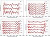 |
Fig. A.1. Comparision of our mean spectra and standard deviations (red) to those of Liu et al. (2016) (black). |
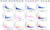 |
Fig. A.2. Evolution of line velocities of in the four subtypes of SESNe. In each figure, different subtypes are plotted in distinct colors: green–IIb, blue–Ib, magenta–Ic, orange–Ic-BL. The same supernovae are plotted with symbols shown in the top legend and connected by lines. SN 2016coi and SN 2019ehk are represented in red and cyan, respectively, as their spectral phenotypes differ from the four subclasses. |
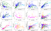 |
Fig. A.3. Evolution of line intensities (pEW) of in the four subtypes of SESNe. Data points follow the same color/symbol scheme as in Fig. A.2. |
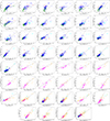 |
Fig. A.4. Correlation of line velocities of SESNe. The blask dashed line in each panel denotes equal velocities of the two lines. Data points follow the same color/symbol scheme as in Fig. A.2. |
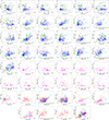 |
Fig. A.5. Correlation of line intensities of SESNe. Data points follow the same color/symbol scheme as in Fig. A.2. |
Information of SESNe observed in the THU sample.
Journal of spectroscopic observations of our SESNe sample.
All Tables
All Figures
|
Fig. 1. Pie charts of the numbers of SNe (left) and numbers of spectra (right) by type. |
| In the text | |
|
Fig. 2. Distribution of the SN redshift (upper left panel), number of spectra for a single SN (upper right panel), phases of spectra (lower left panel), and the phase of the first spectrum of each SN (lower right panel). |
| In the text | |
|
Fig. 3. Preprocessing method for our spectral data. (a) Input spectrum after corrections of redshift. (b) Spectrum after binning into logarithmic scale with dλln = 0.0015. (c) Smoothed spectrum with a window length of 21. The pseudo-continuum is plotted as a dotted line. (d) Spectrum normalized by dividing the continuum in (c). |
| In the text | |
|
Fig. 4. Distribution of tmax, V − tmax, B vs. Δm15, B of our SESN sample. The vertical lines mark the average delay (solid line) and 1σ range (dashed lines). Different types are plotted in different colors, which are denoted in the upper right corner. |
| In the text | |
|
Fig. 5. Schematic diagram illustrating the method of defining the spectral line range. For the smoothed spectrum (upper panel), the first derivative of flux with respect to wavelength is computed (lower panel). Local maxima and minima are identified where the sign of the derivative changes, marked with red upward-pointing and blue downward-pointing triangles, respectively. At certain wavelengths, distinct inflection points are observed where the derivative approaches zero without a sign change; these are indicated by green upward-pointing triangles. The wavelength range of the Hα line is thus delineated in purple, while the local pseudo-continuum is represented by the dashed black line. |
| In the text | |
|
Fig. 6. Mean spectra and their corresponding standard deviations of different subtypes of SESNe at four different phases spanning from –10 to 40 days since V-band maximum. The numbers on the right side of each set of spectra are the corresponding phases, and number of spectra included to calculate the mean spectra is shown in the brackets. The mean spectra are shown by solid black lines, and the 1σ uncertainty is shown by shaded gray regions. Each single spectrum is plotted in light green. For each spectrum, the lines are marked by colors denoted at the top of each figure. |
| In the text | |
|
Fig. 7. Spectral evolution (upper) and line properties (lower) of the double-peaked type Ic SN 2013ge. The different spectral lines are denoted with the colors indicated in the upper panel. |
| In the text | |
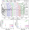 |
Fig. 8. Same as Fig. 7 but for the He-rich broad-lined SN 2016coi. |
| In the text | |
|
Fig. 9. Upper: Normalized spectra of SNe Ib in our sample till maximum light in the range of 5000–7000 Å, showing the features around Hα. The spectra of different SNe are plotted in distinct colors and shifted vertically for better illustration. The main absorption features are highlighted with distinct colored shaded areas. The green bands in the areas denote an absorption line of ambiguous origin that appears concurrently with the blue-wing structure. Lower: Normalized spectrum of SN 2015ah at −8-d showing the range of the doublet feature near 6200 Å. Synthetic spectra by SYNOW with either HI (solid red line) or Si II (dashed blue line) are also overplotted. |
| In the text | |
|
Fig. 10. Pseudo-equivalent widths and velocities of the red-wing feature (attributed to Si IIλ6355) and Fe II lines in the spectra of SNe Ib compared with SNe Ic and Ic-BL. Different subtypes are color-coded, including the peculiar objects SN 2016coi and SN 2019ehk. The data points belonging to the same SN are connected by lines, and those measured from WiseRep spectra are shown with empty symbols. Each SN Ib is represented by a distinct symbol denoted in the legend of (b). |
| In the text | |
|
Fig. 11. Same as Fig. 10, but the red-wing feature attributed to Hα in the spectra of SNe Ib and compared with SNe IIb. The data points circled in (a) correspond to phases later than +10 days. See the main text for details. |
| In the text | |
|
Fig. 12. Spearman’s rank correlation coefficients (ρ) between the measured velocities of lines of different types of SESNe. The ions are arranged such that lighter elements are positioned toward the right and top. The numbers in each box show the coefficients of the corresponding line pairs. Boxes in gray show low statistical significance with a p value higher than 0.05. These cases are all due to the very small dataset. The numeric values are indicated by the color bar at the top of the figure, with lighter colors indicating stronger correlation. Data behind the figure are available at the CDS. |
| In the text | |
|
Fig. 13. Same as in Fig. 12, but for measurements of pEWs of each line. Data behind the figure are available at the CDS. |
| In the text | |
|
Fig. 14. Top: Nebular spectra of SNe Ib (black) and one type IIb (green). Bottom: Nebular spectra of SNe Ic (black), and the peculiar He-rich broad-lined SN 2016coi (cyan). The SN names and the corresponding phases are displayed below each spectrum. |
| In the text | |
|
Fig. 15. Distribution of L[NII]/L[OI] and L[OI]/L[CaII] measured from the nebular-phase spectra of our sample. The data from literature are plotted as empty symbols (Fang et al. 2019). |
| In the text | |
|
Fig. A.1. Comparision of our mean spectra and standard deviations (red) to those of Liu et al. (2016) (black). |
| In the text | |
|
Fig. A.2. Evolution of line velocities of in the four subtypes of SESNe. In each figure, different subtypes are plotted in distinct colors: green–IIb, blue–Ib, magenta–Ic, orange–Ic-BL. The same supernovae are plotted with symbols shown in the top legend and connected by lines. SN 2016coi and SN 2019ehk are represented in red and cyan, respectively, as their spectral phenotypes differ from the four subclasses. |
| In the text | |
|
Fig. A.3. Evolution of line intensities (pEW) of in the four subtypes of SESNe. Data points follow the same color/symbol scheme as in Fig. A.2. |
| In the text | |
|
Fig. A.4. Correlation of line velocities of SESNe. The blask dashed line in each panel denotes equal velocities of the two lines. Data points follow the same color/symbol scheme as in Fig. A.2. |
| In the text | |
|
Fig. A.5. Correlation of line intensities of SESNe. Data points follow the same color/symbol scheme as in Fig. A.2. |
| In the text | |
Current usage metrics show cumulative count of Article Views (full-text article views including HTML views, PDF and ePub downloads, according to the available data) and Abstracts Views on Vision4Press platform.
Data correspond to usage on the plateform after 2015. The current usage metrics is available 48-96 hours after online publication and is updated daily on week days.
Initial download of the metrics may take a while.