| Issue |
A&A
Volume 709, May 2026
|
|
|---|---|---|
| Article Number | A210 | |
| Number of page(s) | 17 | |
| Section | Extragalactic astronomy | |
| DOI | https://doi.org/10.1051/0004-6361/202558180 | |
| Published online | 19 May 2026 | |
J-PAS: Unprecedented precision in stellar populations of diffuse tidal features
1
Centro de Estudios de Física del Cosmos de Aragón (CEFCA), Plaza San Juan 1, 44001, Teruel, Spain
2
Unidad Asociada CEFCA-IAA, CEFCA, Unidad Asociada al CSIC por el IAA, Plaza San Juan 1, 44001, Teruel, Spain
3
Instituto de Astrofísica de Canarias, Calle Vía Láctea s/n, 38205, La Laguna, Spain
4
Departamento de Astrofísica, Universidad de La Laguna, 38205, La Laguna, Spain
5
Instituto de Astrofísica de Andalucía (IAA), Consejo Superior de Investigaciones Científicas (CSIC), Apdo 3004, E-18080, Granada, Spain
6
Instituto de Física de Cantabria (IFCA), CSIC-Univ. de Cantabria, Avda. los Castros, s/n, E-39005, Santander, Spain
7
Observatório Nacional, Ministério da Ciencia, Tecnologia, Inovação e Comunicações, Rua General José Cristino, 77, São Cristóvão, 20921-400, Rio de Janeiro, Brazil
8
Departamento de Astronomia, Instituto de Física, Universidade Federal do Rio Grande do Sul (UFRGS), Av. Bento Gonçalves, 9500, Porto Alegre, R.S, Brazil
9
Donostia International Physics Center (DIPC), Manuel Lardizabal Ibilbidea, 4, San Sebastián, Spain
10
Departamento de Astronomia, Instituto de Astronomia, Geofísica e Ciências Atmosféricas, Universidade de São Paulo, São Paulo, Brazil
11
Instruments4, 4121 Pembury Place, La Canada Flintridge, CA, 91011, USA
12
ARAID Foundation, Avda. de Ranillas, 1-D, E-50018, Zaragoza, Spain
13
Laboratoire d’Astrophysique, École Polytechnique Fédérale de Lausanne (EPFL), 1290, Sauverny, Switzerland
14
GEPI, Observatoire de Paris, CNRS UMR 8111, Université Paris Diderot, 92125, Meudon Cedex, France
15
Lund Observatory, Division of Astrophysics, Department of Physics, Lund University, SE-221 00, Lund, Sweden
16
Departamento de Física de la Tierra y Astrofísica, Facultad de Ciencias Físicas, Plaza Ciencias, 1, 28040, Madrid, Spain
17
Leiden Observatory, Leiden University, J.H. Oort Building, Niels Bohrweg 2, 2333 CA, Leiden, Netherlands
18
National Astronomical Observatory of China, Chinese Academy of Sciences, Beijing, China
★ Corresponding author: This email address is being protected from spambots. You need JavaScript enabled to view it.
Received:
19
November
2025
Accepted:
10
March
2026
Abstract
Galaxies frequently interact with nearby systems, which can significantly alter their morphology and star formation activity. However, spectroscopic studies of their faint and diffuse remnants require very long exposure times and often exceed the limited field of view of integral field units (IFUs). On the other hand, broadband imaging can have a much wider field of view, but it lacks the spectral resolution to identify key spectral features, restricting accurate constraints on stellar population properties. With its 54 narrowband filters in the optical and wide coverage (8000 square degrees, planned), J-PAS fills this gap. In this case study, we examined PGC 3087775, a massive galaxy at z = 0.046179 (∼201 Mpc) in the later stages of a major merger in the J-PAS Early Data Release. Photometry was performed on visually identified polygons (over the tidal features) using Gnuastro and validated with MaNGA IFU data (for the central part). Spectral energy distribution (SED) fitting was then carried out with CIGALE to derive stellar population properties using both J-PAS and SDSS photometry to assess the added value with J-PAS. SDSS indicates a metal-rich population with an extended star formation history (SFH) and elevated star formation rates. J-PAS instead points to a less metal-rich population with moderate extinction and a more rapid SFH, consistent with a quenched stellar population. The average Dn(4000) index of the tidal features is 1.24, suggesting that it was a non-dry merger and a fourfold improvement in the precision of stellar mass and Dn(4000) was found with J-PAS. We also assessed two heuristic methods for estimating the mass-to-light ratio from SDSS filters and found that they overestimate the stellar mass in this galaxy by 0.5 dex and 0.4 dex relative to SED fitting results from J-PAS and SDSS, respectively. Future work will extend this analysis to a larger sample of merging galaxies and evolution of the stellar populations of such structures across the nearby Universe with unprecedented detail. This project and its results are fully reproducible, through Maneage (commit f2cb27a).
Key words: galaxies: interactions / galaxies: irregular / galaxies: photometry / galaxies: structure
© The Authors 2026
 Open Access article, published by EDP Sciences, under the terms of the Creative Commons Attribution License (https://creativecommons.org/licenses/by/4.0), which permits unrestricted use, distribution, and reproduction in any medium, provided the original work is properly cited.
This article is published in open access under the Subscribe to Open model. This email address is being protected from spambots. You need JavaScript enabled to view it. to support open access publication.
1. Introduction
The prevailing theory of galaxy evolution suggests that galaxies grow through a combination of gas accretion and interactions with other galaxies, including both minor and major mergers (Kauffmann et al. 1993; Cole et al. 2000; Bullock & Johnston 2005; Stringer & Benson 2007; L’Huillie et al. 2012). Minor mergers induce significant morphological changes in the smaller galaxy; stripping its stars and gas to form tidal structures around the larger galaxy which is much less affected (Martínez-Delgado et al. 2010, 2023b). In contrast, major mergers typically involve significant perturbations in the interacting galaxies, often accompanied by thick and massive tidal features in comparison to those produced by minor mergers (Weilbacher et al. 2018). These tidal features, which appear as low surface brightness (LSB) structures, can serve as tracers of the stellar populations of the progenitor galaxies (Arp 1966; Toomre & Toomre 1972; Malin & Carter 1980; Quinn 1984; Hood et al. 2018; Miró-Carretero et al. 2023, 2024, 2025). A systematic search for tidal stream features, combined with a comprehensive characterization of their stellar populations – including ages, masses, and star formation histories (SFHs) – is crucial for advancing the field, as it sheds light on the hierarchical assembly and evolutionary history of galaxies and provides valuable constraints on the nature of dark matter (Fall & Efstathiou 1980; van den Bosch et al. 2002; Agertz et al. 2011).
So far, most studies of the photometric properties of tidal remnants have employed broadband filters (Javanmardi et al. 2016; Miró-Carretero et al. 2023; Laine et al. 2024; Martínez-Delgado et al. 2024; Miró-Carretero et al. 2024, 2025) because they offer deep imaging across wide areas. However, such filters lack the spectral resolution required for precise characterization of stellar populations. While spectroscopy can overcome this limitation, observing diffuse tidal structures remains challenging due to the impractically long exposure times needed, even at low resolutions. Furthermore, the limited fields of view of integral field units (IFUs) restrict our ability to fully map extended features. For instance, Mapping Nearby Galaxies at APO (MaNGA; Bundy et al. 2015; Cherinka et al. 2019), which uses the Sloan 2.5 m telescope, is only 12 − 32 arcsec in diameter; the PMAS/PPAK at Calar Alto, used in surveys such as Calar Alto Legacy Integral Field Area (CALIFA; Sánchez et al. 2012), provides a hexagonal shape of 74 × 64 arcsec2; and the Multi Unit Spectroscopic Explorer (MUSE; Bacon et al. 2010) at the Very Large Telescope (VLT) covers just 59.9 × 60 arcsec2. These constraints often necessitate multiple pointings for the study of nearby galaxies (e.g., in PHANGS-MUSE; see Emsellem et al. 2022) or preselection of specific regions within the tidal structures (Zhou et al. 2014; Zaragoza-Cardiel et al. 2018; Weilbacher et al. 2018; Zhang et al. 2020; Martínez-Delgado et al. 2024).
The Javalambre Physics of the Accelerating Universe Astrophysical Survey (J-PAS; Benitez et al. 2014) bridges the gap between broadband imaging and spectroscopy through its innovative design. J-PAS employs 54 contiguous narrowband filters to obtain a low-resolution spectral energy distribution (SED; R = 39 − 90) for every pixel across its planned 8000 deg2 coverage of the northern sky. This is achieved without any preselection, thereby enabling SED-based selection, or an un-biased SED analysis of extended tidal features for the first time.
To understand the additional advantages of J-PAS for these features, in this work, we used the J-PAS Early Data Release (EDR; Vázquez Ramió et al., in prep.) to investigate the merging galaxy with the brightest tidal features within the J-PAS EDR footprint: PGC 3087775 (hereafter Alba; see Fig. 1). It is cataloged in the J-PAS EDR as 9601-18620 and has a spectroscopic redshift of 0.046179 according to NASA/IPAC Extragalactic Database (NED), based on data from the DESI Collaboration (2024). Alba is also cataloged as PGC 3087775, 2MASX J16270254+4328340, SDSS J162702.56+432833.9, and MaNGA 1-134964, among others. Assuming Planck 2018 cosmology (where H0 = 67.66 km s−1 Mpc−1, ΩΛ = 0.6889 and Ωm = 0.3111; Planck Collaboration VI 2020), Alba is approximately 201 Mpc away. Alba is also classified as a Seyfert 2 active galactic nucleus (AGN, Toba et al. 2014) in Set of Identifications, Measurements and Bibliography for Astronomical Data (SIMBAD)1 (Wenger et al. 2000). Alba is characterized by prominent, thick tidal features extending over 56 kpc, identifying it as a multicomponent system in the advanced stages of a major merger (Petersson et al. 2023). This makes Alba an ideal case study for evaluating the consistency of stellar population properties derived from different datasets, specifically J-PAS and Sloan Digital Sky Survey (SDSS; used in deep imaging surveys such as HSC, Legacy Survey or LSST), using various analytical methodologies.
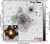 |
Fig. 1. Alba galaxy (PGC 3087775) and its major merger remnants. The main panel shows surface brightness image of the Alba galaxy that is produced by co-adding all 57 J-PAS bands (including 54 narrowband filters, two medium-band filters, and one broadband filter; however, only the 56 narrow and medium-band filters are used in the analysis presented in this paper). The co-add reaches a 3σ mSBL over 100 arcsec2 of 29 mag/arcsec2. The color bar represents the surface brightness of the co-added image. The hexagon over the center of the galaxy delineates the MaNGA footprint used to validate J-PAS SEDs in Fig. 2. The six polygons delineated with the thin lines, are named and studied independently in subsequent figures (with the same color-coding). The lower left panel displays a false-color image from the HSC-SSP (Subaru) wide survey, created using the z, r, and g filters as the red, green, and blue. Polygon coordinates are on Zenodo (see Appendix E.1). |
In this paper, we assess the stellar population properties of the tidal features based on their physical criteria, including the spatial configuration and morphology of the tidal structures, as well as the presence of emission or absorption lines within different parts of the merger remnant. The two primary approaches employed are SED fitting and the following two heuristic methods for obtaining the stellar mass from SDSS filters: Bell et al. (2003, hereafter B03) and García-Benito et al. (2019, hereafter GB19). Heuristic methods have been widely adopted in the literature to estimate stellar mass-to-light (M/L) ratios, making them relevant for this work.
This paper is organized as follows. Sect. 2 introduces the datasets used, and Sect. 3 details the analytical approach and the tools employed for data processing and interpretation. In Sect. 4, we present the results, which are followed by a discussion of their implications in Sect. 5. Finally, Sect. 6 provides a summary of the key findings, highlights the main contributions of the study, and offers concluding remarks.
2. Data
J-PAS employs an innovative filter system comprising 54 narrowband filters (14 nm wide), complemented by two medium-band filters (on the extreme blue and red) to encompass the entire optical spectrum from 3216 Å to 10 839 Å, see Fig. 2 of Bonoli et al. (2021). Furthermore, J-PAS also has one broadband filter (iSDSS) that is used as the detection filter in its main catalog. The non-overlapping J-PAS spectral resolution element (only the narrow-bands) is 10 nm, across the wavelength range from 390 nm to 900 nm.
J-PAS is observed from the Observatorio Astrofísico de Javalambre (OAJ) using the Javalambre Survey Telescope (JST250 with a 2.5 m mirror) that has an impressive effective field of view spanning seven square degrees (3.5 square degrees exposed). In this work, we employed images from the J-PAS EDR, which covers an effective area of ∼12 square degrees in all filters. Details of the dataset including the mean full width at half maximum (FWHM) of the point spread function (PSF), exposure times for each tray, and so on, are thoroughly described in Vázquez Ramió et al. (in prep.).
The Alba galaxy was detected in the co-added images of all 57 filters. These co-adds combine 482 individual exposures obtained between 29 June 2023 and 6 April 2024. The observing conditions of the contributing frames cover a broad range, with image quality characterized by a median FWHM = 0.99″. Individual exposure times are 60 s in all filters, except for the iSDSS band where 30 s exposures are used in order to minimize saturation. The signal-to-noise ratio (S/N) of the individual detections of the Alba galaxy spans from 21 to 588, with a median value of 185. As expected, the highest SNR is reached in the iSDSS band. For the narrowband filters, the S/N follows the combined effect of the instrumental throughput and the SED of the source.
To assess the performance and validate the capabilities of J-PAS, we employed data from the MaNGA survey (Bundy et al. 2015; Cherinka et al. 2019), which provides spatially resolved spectroscopic data for a large sample of nearby galaxies. In addition, we utilized imaging data from the SDSS Data Release 9 (Blanton et al. 2017), which provides observations in five broadband filters: u, g, r, i, and z. We chose to use SDSS data for several reasons. Firstly, it offers a depth comparable to that of J-PAS. Secondly, SDSS (or SDSS-like) filters are used extensively within many other surveys, thereby facilitating comparison and consistency with previous studies.
The Subaru Hyper Suprime-Cam Subaru Strategic Program (HSC-SSP) Data Release 2 (Aihara et al. 2019) was also used as a much deeper dataset to precisely identify and draw the polygons that trace the tidal features. These are also shown in Fig. 1 for a better visual demonstration of Alba. The 3σ surface brightness limit in the HSC-SSP g band, measured over an area of 100 arcsec2, is 30.31 mag/arcsec2.
3. Analysis
3.1. Photometry and region definitions
Photometry was conducted using GNU Astronomy Utilities (Gnuastro2; Akhlaghi 2025), a comprehensive software suite comprising various programs and library functions designed for the manipulation and analysis of astronomical data. All programs share a unified command-line interface, enhancing usability for both end users and developers. Moreover, Gnuastro strictly complies with GNU coding standards, facilitating smooth integration with Unix-based operating systems and existing shell scripts. A particular Gnuastro program that is important in this analysis is MakeCatalog (Akhlaghi 2019b), which features the executable command astmkcatalog. This program accepts labeled images to use as apertures of various shapes (non-parametric) and generates a catalog of measurements over each label.
To generate the detection map and effectively separate the signal from the noise, we employed NoiseChisel (Akhlaghi & Ichikawa 2015); to mask the foreground and background contaminants, we used the Segment program (Akhlaghi 2019a). The segmentation map used for masking was then obtained from the co-added image of all 57 J-PAS filters (54 of which are narrowband filters, two are medium-band filters, and one is a broadband filter). The “clumps” of Segment over the polygons in the deeper image (background galaxies or foreground stars) are masked with the same method shown Fig. 5 of Martínez-Delgado et al. (2023a), and we checked that no residual flux remained. The masks were then applied to the photometry in the 56 narrow and medium bands to avoid the contamination of foreground and background sources that are not part of the tidal features. The PSF of each filter is slightly different, but because we masked all resolved sources over the streams and their area is much larger than the PSF, the wavelength dependence of the PSF does not affect our analysis (for further details regarding the PSF-subtraction procedure, see Eskandarlou et al. 2026).
The differing pixel grids of the different surveys are warped to the pixel grid of J-PAS using the –gridfile option of Gnuastro’s Warp program, see Sect. 6.4 of Akhlaghi (2025). In addition, we utilized the astscript-color-faint-gray to generate a color image (Infante-Sainz & Akhlaghi 2024)3.
To identify different regions of the major merging system, we manually draw the named polygons of Fig. 1 with SAOImage DS9 (Joye & Mandel 2003). They were drawn over the deeper HSC images, based on morphological differences and spatial continuity, in order to effectively separate the various structural components. Namely, the HSC images are only used to create the labeled images. The measurements (over those labels) are done on the values of pixels from J-PAS and SDSS using the MakeCatalog. The stellar population properties further described below within Alba’s streams were estimated using this photometry.
The polygons were not generated through an automated image segmentation algorithm in this paper. This is because any such algorithms will also have systematics that need to be studied in detail, but that is beyond the scope of this work (on the stellar population properties of a new filter set rather than on the methodological optimization of stream extraction algorithms). A comparison between visually defined regions and those identified using automated segmentation algorithms constitutes an important avenue for future work on a larger sample of galaxies.
3.2. J-PAS comparison with MaNGA
To validate J-PAS calibration and our photometry, Fig. 2 compares the J-PAS photometry with MaNGA spectroscopy over the MaNGA footprint shown in Fig. 1. To further assess the reliability of J-PAS measurements, we down-sampled the MaNGA spectrum using the J-PAS filter set. In the literature, this down-sampling is sometimes called “convolution”, because applying the filter transmission curve to spectra shares some similarities with a convolution kernel. However, this term can lead to confusion because convolution does not alter the sampling, it only changes the resolution (the number of elements remains the same). Furthermore, in convolution the kernel moves, but it is fixed in this usage.
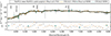 |
Fig. 2. Validation of J-PAS SEDs using MaNGA spectroscopy in the central region of the Alba galaxy (shown in Fig. 1). Top: Gray line indicates the MaNGA spectrum in this area, and the black line shows it after down-sampling with J-PAS filter throughputs. The orange points correspond to the measured J-PAS SED, and the solid orange line illustrates the best-fitting SED model derived from J-PAS data in the same region (after applying a minor constant correction factor of ×1.09 to all filters). Similarly, the teal triangles indicate the measured SDSS SED, and the solid teal line shows the corresponding SDSS SED fit (following the application of a small constant correction factor of ×0.96 to all filters). Some spectral line positions at the Alba galaxy redshift are also shown. Bottom: Percentage difference between the down-sampled MaNGA spectra and the J-PAS photometric data. This validates the very good calibration of J-PAS and allowed us to study regions beyond the small footprint of MaNGA. Furthermore, the orange and teal points and triangles represent the residuals between the SED fits derived from J-PAS and SDSS, respectively, and their corresponding observed fluxes. The dataset used to produce this plot can be accessed at Zenodo (see Appendix E.2). |
The MaNGA spectrum in Fig. 2 lacks the typical AGN emission lines, such as [O III]; instead, only [O II] and [N II] are detected, leading to its classification as a low-ionization nuclear emission-line region (LINER; Albán & Wylezalek 2023) galaxy. No significant differences are observed between J-PAS and the down-sampled MaNGA data in Fig. 2. Furthermore, Fig. 2 presents a comparison between the SED fitting results derived from J-PAS and those obtained from SDSS; this comparison is discussed in greater detail in Section. 3.3.
The minor differences between the down-sampled MaNGA and J-PAS occur on absorption lines. The MaNGA observations (April 2015) and J-PAS data (July 2023) are separated by a substantial temporal gap. However, the differences cannot be attributed to temporal variability of AGNs. This is because variability is a behavior characteristic of Seyfert 1 nuclei due to changes in the broad-line region, but it is not the case for Seyfert 2 nuclei (the case for Alba). Furthermore, the absorption in Hβ shows the strongest difference between MaNGA and J-PAS. However, Hβ originates from the underlying stellar population rather than the AGN, and is not expected to have variability on this timescale. The difference on absorption lines is therefore most plausibly explained by measurement uncertainties rather than intrinsic variability. A global scaling factor of 1.09 was applied to the J-PAS fluxes, while a factor of 0.96 was used for the SDSS fluxes in order to place both datasets on the same absolute scale as the MaNGA measurements. Such rescaling is a common procedure when combining photometric and spectroscopic observations, as systematic differences frequently arise from variations in aperture size, calibration methods, and the FWHM between the respective instruments and observational techniques (e.g., Logroño-García et al. 2019). The most significant outcome of this procedure is the strong agreement in the resulting SED shape. Specifically, the comparison indicates that the SED derived from J-PAS and SDSS photometry is consistent with the spectroscopic measurements at approximately the 4% level, demonstrating a high degree of reliability in the cross-calibration between the datasets.
Having validated the J-PAS photometry on the overlapping region with MaNGA, we then extended our analysis to the outer tidal features, where no IFU spectroscopy is available. Fig. 3 shows the J-PAS photometry (in units of surface brightness) of different polygons over the tidal features from Fig. 1, in both wavelength flux density (top) and AB magnitudes (bottom). Recall that the AB-magnitude system is based on the frequency flux density. It is important to show both units, as the two communities (IFU and wide-field broadband imaging) use different conventions and the conversion is not linear. From the bluer to the redder filters, the slope of the wavelength flux density increases, whereas the slope of the AB magnitude decreases. This occurs because of the inverse relationship between wavelength and frequency in the two units. Compared to Fig. 2, the S/N in the center of Alba is 20 times higher than in the tidal streams; hence, the error bars are more visible there.
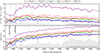 |
Fig. 3. SED (in surface brightness) of different sections of the tidal feature, presented in two units. The top panel features units of wavelength flux density (used in the IFU community) of the six distinct polygons, while the lower panel features units of AB magnitude (used in the imaging community). The colors in this plot correspond to those used in Fig. 1 to represent different polygons. The gray bars at the bottom of each plot show the 3σ mSBL for each filter over an area of 100 arcsec2. The data used to generate this plot are available on Zenodo (see Appendix E.3). |
Fig. 3 also shows the measured surface brightness limit (mSBL, defined in Sect. 7.4.5.1 of Akhlaghi 2025), which is represented by gray bars. The mSBL of each filter is shown in the two units for a general understanding of J-PAS capabilities regarding the low surface brightness regime, this is not specific to Alba. For example, in the two bluest filters, the measured flux of some of Alba’s tidal features become fainter than the mSBL. This is not a cause for concern because the polygon areas are considerably larger than the 100 arcsec2 used to estimate the mSBL, with the smallest area being at least three times greater. Furthermore, the mSBL is measured on the noise ( ; where A is the area in number of pixels), while the fluxes are measured on signal (∼A). Ultimately, later processing (SED fitting) accounts for the different error bars of each filter, so the larger error bars of the two bluest filters will not have a significant impact on the conclusions of this paper. In contrast, the mSBL in the red filters (redder than 7200 Å) is brighter due to the presence of telluric emission lines from the atmosphere, which introduce increased Poisson noise.
Additionally, in Fig. 3, the North-2 polygon appears significantly elevated relative to the other tidal streams. This is consistent with the color image in Fig. 1, where North-2 is visually brighter than the other regions and has a smaller area, confirming its higher surface brightness.
3.3. SED fitting
We employed the Code Investigating GALaxy Emission (CIGALE; version 2022.0; Boquien et al. 2019) to perform SED fitting in each of the polygon regions defined in Fig. 1. CIGALE is grounded in the principles of energy balance and utilizes a Bayesian-like statistical framework. CIGALE is specifically designed to investigate galaxy evolution by comparing modeled SEDs with observed data across a broad wavelength range, from X-rays and far-ultraviolet to far-infrared and radio frequencies. An important feature of CIGALE for us is its ability to simultaneously model both stellar continuum emission and ionized gas (emission lines). Although Alba’s tidal features do not show strong emission lines, this capability will be crucial for future studies of merging galaxies in J-PAS where the outskirts may contain significant emission from stripped gas, circumgalactic inflows, or nuclear outflows. J-PAS is well suited to detect such features in the local Universe.
The input to CIGALE for each polygon consists of flux measurements and their associated uncertainties, derived from the 56 medium and narrow J-PAS bands (the broadband filter is excluded in the SED fitting) and SDSS (five broadband filters), represented as colored circles and gray triangles, respectively, in Fig. 4. The resulting CIGALE-fitted spectra are shown by solid lines in Fig. 4. The spectra and circles show the J-PAS-derived results and follow the same color-coding of the polygons in Fig. 1. The gray spectra and triangles are derived from SDSS. Additionally, Fig. 2 presents both the flux measurements and the corresponding SED-fitting outputs from CIGALE: the J-PAS results are indicated by orange dots and a solid orange line, whereas the SDSS results are shown using teal triangles and a solid teal line.
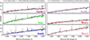 |
Fig. 4. SED fitting on Alba’s tidal features. The measured SEDs and fitted spectra of the left and right panels show the inputs and outputs of CIGALE for both J-PAS and SDSS. They correspond to the named polygons of Fig. 1 with the same color. Circles show fluxes from 56 narrow/medium-band J-PAS filters, while triangles represent SDSS’s five broad filters. Fitted CIGALE spectra are overlaid using gray (SDSS) and colored (J-PAS) lines. The residuals between the SED fitting results of both surveys and their respective observed fluxes are presented in Appendix. A (Fig. A.1). The dataset underlying this plot is publicly accessible through Zenodo (see Appendix E.4). |
The stellar population parameters derived by CIGALE are provided in two forms: “best-fit” estimates and “Bayesian” values, the latter are accompanied by corresponding uncertainties. In our analysis, we employed the Bayesian values. For our SED fitting, we adopted libraries of single stellar populations from the BC03 module (Bruzual & Charlot 2003) and used the sfhdelayed module. This module defines an analytic SFH based on a delayed model that may include an optional exponential burst (which could have been induced by the merger); assuming a Chabrier (2003) initial mass function (IMF). In addition, we also ran CIGALE with the Salpeter (1955) IMF for later comparison with heuristic M/L methods (discussed in Sect.4.2 and Appendix C) and with a disabled burst and nebular emission to assess their impact on the results below (see Appendix D).
To set the CIGALE parameters (see Appendix B), we used an iterative approach. At first, we used broad age_main bins and then refined them according to the first results. For instance, the early runs showed that the age_main value was between 4000 and 5500 Myr. After that, we narrowed the bins around this range and gradually increased the time resolution until the error bars became stable and the age_main value remained unchanged. This systematic adjustment of the input parameters ensured consistency between the Bayesian and the best-fit results.
We explored all the remaining available CIGALE configuration options and carefully adjusted the input parameters in incremental steps to achieve the best fit. The grid parameters that were modified in this analysis are listed in Appendix. B. The output properties4 reported in Table 1 correspond to the following CIGALE output columns: E(B − V)s (bayes.attenuation.E-BVs; E(B − V)s, the color excess of the stellar light for both the young and old populations), Dn(4000) (bayes.param.D-4000; D4000 break using the Balogh et al. (1999) definition), age burst (bayes.sfh.age-burst; age of the late burst), age main (bayes.sfh.age-main; age of the main stellar population in the galaxy), fraction burst (bayes.sfh.f-burst; mass fraction of the late burst population), Z (bayes.stellar.metallicity; metallicity), star formation rate (SFR; bayes.sfh.sfr; instantaneous SFR), M★ (bayes.stellar.m-star; total stellar mass), τBurst (bayes.sfh.tau-burst; duration (rectangle) or e-folding time of all short events), and τMain (bayes.sfh.tau-main; e-folding time of the main stellar population model). A comprehensive description of these output parameters and their physical interpretations is provided by Boquien et al. (2019).
CIGALE best-fit parameters.
To assess the reliability of the CIGALE errors, we introduced Gaussian noise with a standard deviation of 1σ (where σ represents the error in measured flux from MakeCatalog). This process was repeated 100 times for each polygon, implemented via the mknoise-sigma operator of Gnuastro’s Arithmetic program. Since we studied seven different polygons (including the central region), the procedure resulted in a large table containing 700 rows of simulated error values. We then ran CIGALE for these 700 random flux errors using both J-PAS and SDSS data. The results suggest that the error bars provided by CIGALE are accurate. For instance, in the case of the east polygon, the stellar mass derived from the 700 random flux variations was 9.44 ± 0.02 for J-PAS and 9.62 ± 0.05 for SDSS. These results are consistent with the error bars directly provided by CIGALE (see Table 1), which report 9.44 ± 0.02 for J-PAS and 9.63 ± 0.06 for SDSS.
For some of the merger remnants, the SDSS fluxes and fitted SEDs in the blue filters are lower than those obtained from J-PAS, whereas in the redder filters they can be higher. This discrepancy could arise from photometric reduction issues affecting specific SDSS filters, although the possibility of an underlying systematic effect cannot be entirely excluded. Importantly, this behaviour is not observed in all polygons. Given the substantially larger number of filters employed by J-PAS, the impact of potential photometric systematics in any single filter is significantly less than SDSS. Consequently, systematic effects in individual filters are less likely to introduce pronounced biases in the reconstructed SED compared to analyses based solely on SDSS data.
A noticeable difference between the SED fittings derived from J-PAS and SDSS fluxes is that the SDSS fitting for the east and south regions display numerous emission lines, that are not visible in J-PAS fitting. Given that the SDSS SED fitting reveals such features, while Alba does not demonstrate such strong emission or absorption lines in J-PAS photometry in the merger remnants (even in the central regions of the galaxies), the presence of so many emission lines in the SDSS data highlights the need for further investigation. Therefore, we reran CIGALE with the starburst and nebular emission components disabled (see Appendix D). We found that, after removing these components, the CIGALE output properties studied (for the stellar population, not gas or emission lines) remained largely unaffected. This outcome is most likely attributable to the stellar populations in the tidal features and the lower spectral resolution of SDSS. As the extra emission lines in the two polygons do affect the central argument of this paper (which is primarily concerned with stellar populations, not gas emission), all subsequent CIGALE analyses were conducted with the starburst and nebular emission components enabled.
4. Results
A unique feature of J-PAS is its ability to identify galaxies and their tidal structures based on spectral characteristics and stellar population properties without the need for preselection, thus operating in a fully blind manner. This paper serves as a proof-of-concept case study that will later be expanded to encompass a larger sample of galaxies. In the following subsections, particular emphasis is placed on the stellar populations, comparing the results obtained from J-PAS with those derived from SDSS, followed by a study of the self-consistency of the SED fitting results between J-PAS and SDSS. Finally, we focused on stellar masses with a comparison of the results from SED fitting with two heuristic methods that are commonly used in the literature (with broadband photometry).
4.1. Spectral energy distribution fitting properties from J-PAS and SDSS
In principle, Alba’s current state should have a single narrative. However, when analyzed using J-PAS and SDSS, different interpretations emerge. Some properties are constrained by both datasets, others are constrained by only one, and certain parameters remain unconstrained in both cases. Table 1 summarizes the physical properties inferred from the SED fitting of both surveys, while Fig. 5 provides a corner plot to visually compare these parameters. In this plot, teal points denote the J-PAS results, while orange points correspond to those from SDSS.
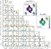 |
Fig. 5. Corner plot showing the pairwise comparison of SED fitting output properties for J-PAS (teal circles) and SDSS (orange circles). In this analysis, all starburst and nebular components are included, and the Chabrier (2003) IMF is applied. Details of the grid parameters are provided in Appendix B. The 2D plots in the top right illustrate the comparison between J-PAS and SDSS in terms of the Dn(4000) index and stellar mass distribution. In addition, the stellar mass derived from SED fitting (from J-PAS and SDSS) is compared using the two following methods: Bell et al. (2003, labeled as B03) and García-Benito et al. (2019, labeled as GB19), both are based on the M/L ratio. The data used to generate this corner plot for both datasets are available on Zenodo (for further details, see Appendix E.6). |
Based on Table 1, both J-PAS and SDSS provide consistent constraints on AgeMain. The derived values and their corresponding error bars are nearly identical in the two datasets, and, on average, the polygons yield an AgeMain value of 4.65 Gyr. In contrast, several parameters are constrained (value larger than the error) only by J-PAS, including Dn(4000), E(B − Vs), and stellar mass, each with noticeably smaller error bars compared to SDSS. This is because J-PAS is able to resolve spectral breaks with better precision, thereby extracting information that SDSS cannot capture as effectively. Nevertheless, a number of parameters remain weakly constrained in both surveys, as reflected in their large uncertainties. These include AgeBurst, metallicity, FBurst, τBurst, and τMain. This is most likely because Alba does not display any significant starburst features in its SED. As a result, these parameters lack physical reliability in this case and cannot be incorporated into our interpretation with confidence. We assume that if Alba was in an earlier phase of its merger (before the more massive stars had died out) these would be better constrained. This hypothesis will be tested in followup studies on a larger sample of mergers.
The main differences observed in the corner plot of Fig. 5 involve metallicity, attenuation, and stellar mass, all of which are lower in J-PAS compared to SDSS. This result is consistent with the redder SED observed by SDSS and may reflect systematic differences in the derivation of these parameters. However, trends such as AgeBurst versus attenuation, AgeMain versus Z, and Z versus attenuation are likely sensitive to degeneracies. In addition, J-PAS produces lower values for the SFR, τBurst, and τMain. For example, SDSS predicts a more extended burst history (both in the τBurst and in the FBurst), leading to higher inferred SFR values. Nevertheless, these interpretations should be approached with caution at this stage. As noted previously, the error bars associated with AgeBurst, τBurst, and τMain are large in both datasets, limiting their reliability for robust physical conclusions, even though the general correlations remain discernible.
It should also be emphasized that this analysis is based on a single case study. A larger statistical investigation of merger remnants will be necessary to confirm and refine these trends. Overall, for Alba’s tidal features, SDSS indicates a metal-richer stellar population with stronger attenuation, a highly extended SFH, and higher SFRs. In contrast, J-PAS suggests a systematically lower metallicity with moderate extinction and a more rapid SFH, consistent with a stellar population that is in an earlier phase of quenching.
As mentioned earlier, several emission lines are evident in the SDSS SED fitting of two polygons shown in Fig. 4; this could imply CIGALE is putting too much significance on the starburst component for the SDSS photometry of Alba and making it hard to compare SDSS stellar populations with those of J-PAS. This serves as a useful check to determine whether the main difference in the fraction of the starburst component derived from the SDSS data arises from degeneracies in the fits, and whether the larger fraction of young stellar components leads to meaningful variations in E(B − Vs) and metallicity. To verify the effect of the starburst component on the comparison, we performed an additional analysis by rerunning CIGALE, this time excluding the starburst and nebular components. Further methodological details are provided in Appendix D, and the corresponding results are presented in Fig. D.1. When looking at panel of E(B − Vs) versus Z in Figs. 5 and D.1, we can confirm that the SDSS values do not change significantly. This can also be verified by the respective error bars in Table 1 (e.g., the error bar in SDSS’s SFR is almost three times larger than the value). This confirms that the emission lines in SDSS fittings are due to degeneracies in the fitting process and have no statistical significance in our analysis.
For the remaining parameters, the variations are minimal. This result is consistent with the fact that Alba exhibits neither significant star formation activity nor strong emission lines. Consequently, even after the exclusion of the starburst components, the changes in properties constrained by J-PAS and SDSS are small, and we cannot see big difference in the constrained properties.
4.2. Self-consistency
In the previous section, we compare J-PAS and SDSS stellar population properties. In this section, we compare the results of each survey separately: seeing which properties in each filter set can be derived with sufficient accuracy in the case of Alba for further study. We therefore attempted to exclude properties that do not exhibit statistically significant variation across the various polygons. In other words, we focused on identifying properties with relatively small error margins in comparison to their variation across the six polygons of Alba.
To do this, we defined the property variation significance (PVS), which is calculated using the standard deviation of each property (e.g., mass, age, etc.) across the six polygons and dividing it by the median of that property’s error bar (also across the six polygons). The formula used is:
 (1)
(1)
The PVS therefore quantifies the significance of the scatter of a property in the various components relative to the representative error of that property. For instance, in the case of stellar mass, the numerator of the equation for J-PAS is 6.37 × 10⁸ M⊙, while the denominator is 2.68 × 10⁸ M⊙ (note that, since we are considering the ratio, the logarithmic mass is not used). This yields a ratio of 2.38σ, indicating that the scatter in this property among the polygons is comparatively high compared to their noise and error. In contrast, for the same property measured using SDSS, the values are 6.30 × 10⁸ M⊙ and 8.98 × 10⁸ M⊙, producing a ratio of 0.70σ. This result suggests that, for SDSS, the variation in stellar mass values across Alba’s tidal features is less significant (harder to interpret) in comparison to J-PAS.
We ranked the output properties studied here according to their PVS5 in Table 2 (sorted by their PVS in J-PAS). In the rest of the paper, properties with PVS < 1.5 are excluded, as their variation across polygons is within the margin of error (less than 1.5σ), rendering their differences unreliable for analysis of the Alba system with the current data and CIGALE run.
Alba is in the later stage of a major merger; hence, the stellar populations of the progenitors are heavily mixed and the most prominent and massive OB stars of a potential burst in star formation (triggered by the merger) have died out. Therefore, it is reasonable that the PVS of some properties like age of burst is not distinguishable (within the error bars) even with J-PAS resolution in Alba. For example, in earlier phases of a non-dry merger (when the OB stars from a possibly induced star formation are still present), J-PAS resolution should be able to determine the age of burst with much smaller errors. Follow-up studies on a larger sample of mergers in J-PAS will be done in our next papers to assess this.
The M★ and Dn(4000) from the J-PAS dataset met the PVS > 1.5 condition, with values of 2.38 and 1.63, respectively. In contrast, none of the output properties derived from SDSS photometry passed this condition. Therefore, for Alba (this case study), our analysis focused on the stellar mass and Dn(4000). Depending on the physical characteristics of different mergers, we employed the PVS framework to identify the properties most affected at the observed phase. In this sense, PVS functions as a calibrator of galaxy mergers, highlighting the properties whose variations are most informative within the constraints of the available data for each galaxy. This approach enabled the classification of merging systems according to their distinctive stellar population or gas and nebula features, a task that was previously unfeasible. For example, once extended to many merging galaxies, we can extract galaxies that exhibit a PVS(Dn(4000)) greater than 1.5 to examine potential correlations with merger dynamics, morphology, or environment.
After evaluating the self-consistency of J-PAS and SDSS and finding the parameters that can yield useful information for Alba, we studied those two parameters. The Dn(4000) index quantifies the strength of the 4000 Å break in the optical spectrum of a galaxy (Balogh et al. 1999), which is primarily influenced by the age and metallicity of its stellar population (Kauffmann et al. 2003; Gallazzi et al. 2005). As demonstrated by Kauffmann et al. (2003), the Dn(4000) index increases as a function of stellar population age. In Fig. 5 (bottom-right panel), we see the Dn(4000) values across the 2D spatial footprint of the Alba galaxy. In J-PAS this spatial distribution shows that the center has the highest value. This is expected in a major merger: the fraction of younger stars in the center is the smallest, since any possible gas in the progenitors was stripped or turned into stars in earlier phases. Also, North-1 has the smallest value that is consistent with its bluer color in the HSC image of Figure 1. However from the SDSS, we see that the center does not have the highest value, and the spatial distribution is hard to interpret.
For Alba, the dominant factor influencing Dn(4000) appears to be the recent major merger event and the resulting star formation (which has become quiescent ever since), which is nevertheless different in each of the polygons (that contain stars from different phases of the merger). Further simulations could help constrain essential merger parameters, such as the mass ratio of the interacting galaxies, the impact parameter, and the time since the merger occurred, but such investigations are beyond the scope of this paper.
The stellar mass (M★) also passed the PVS > 1.5 condition for Alba with J-PAS. In Fig. 5 (top right panel), we present the stellar mass distribution across different regions of the polygons in a 2D map of the Alba galaxy. The J-PAS data show that the stellar mass in the tidal streams is systematically lower (darker colors) than that derived from the SDSS data and has less scatter. Except for these two issues, the overall 2D mass distribution is consistent between J-PAS and SDSS, with the central region being the most massive (with approximately similar masses).
However, calculating the ratio between the diffuse components and the central region to estimate the merger mass ratio is not feasible in this case. Alba is already in a late stage of a major merger, where the central regions of the progenitor systems have coalesced. Consequently, the mass ratio, which is typically determined before coalescence, cannot be reliably derived here.
4.3. Stellar mass from SED fitting and heuristic methods
SED fitting is not the only method employed in the literature to estimate stellar mass from SDSS filters, there are also heuristic methods to only derive the stellar mass; for example, B03 and GB19. Therefore, it is necessary to also evaluate our results with those. B03 has been the most widely used for stellar streams (see, e.g., Martínez-Delgado et al. 2023b and Sola et al. 2025 among many others). However, B03 is based on a Salpeter (1955) IMF, while our default run of CIGALE uses a Chabrier (2003) IMF. We approached this issue in two ways: (1) we used the GB19 heuristic, which also assumes a Chabrier IMF; and (2) we re-ran CIGALE with a Salpeter IMF (see Appendix C).
To derive a heuristic estimate of the stellar mass, we calculated the absolute magnitude of the object in a selected SDSS filter, such as the r band (Mr). As an example, we illustrated the process using the r band; however, the same procedure was applied across all SDSS filters. This calculation incorporates the apparent magnitude, distance modulus, and extinction. We obtained the absolute magnitude of the Sun in the r band M⊙, r, from Willmer (2018). Using the luminosity–magnitude relation, we calculate:
 (2)
(2)
this is for the luminosities of both the object and the Sun in the r band. We then rearranged this equation to yield the luminosity in units of solar luminosity:
 (3)
(3)
We calculated the stellar mass by multiplying the luminosity ratio by the M/L ratio in the r band, using the coefficients provided by B03 (Table A.7) and GB19 (Table B.1). Finally, we obtained the g − r, g − z, and r − z colors and derived the stellar mass for each filter/color combination (yielding 9 masses for the three colors). We used the mean of these colors to determine the M/L ratio and their standard deviation to define the scatter of the distribution, following the methods of Martínez-Delgado et al. (2023b) and Sola et al. (2025). To validate our procedure, we tested our scripts on the magnitudes and colors of Martínez-Delgado et al. (2023b) and successfully reproduced their stellar mass estimates. Fig. 5 presents the results of the stellar mass estimates derived from B03 and GB19 for Alba’s polygons. These are visualized as 2D maps in the stellar mass panel, with the lower left corner showing the B03 results and the lower right corner displaying those from GB19.
The color bar in the plot was adjusted to account for all four displayed results; therefore, the difference between the B03 and GB19 models is not immediately visible. To compare the two methods quantitatively, we converted the stellar masses to a linear scale and found that the B03 estimates are approximately 1.2 times higher than those of GB19. This outcome is expected, as the Salpeter (1955) IMF is bottom-heavy compared to the Chabrier (2003) IMF, naturally resulting in higher stellar mass estimates for B03.
Our default run of CIGALE employed a Chabrier (2003) IMF; therefore, we re-ran the code using a Salpeter (1955) IMF to evaluate its effect on the stellar mass derived for Alba’s streams with J-PAS and SDSS SED fitting (see Fig. C.1 in Appendix C). The analysis shows that adopting the Salpeter (1955) IMF produces stellar masses 1.73 and 1.76 times larger than those obtained with the Chabrier (2003) IMF for J-PAS and SDSS, respectively. This result is consistent across both datasets, as the bottom-heavy Salpeter (1955) IMF naturally yields higher stellar mass estimates than the Chabrier (2003) IMF.
Comparing the heuristic stellar masses with the SED-based stellar masses (J-PAS or SDSS), we see that the heuristic methods produce systematically higher stellar masses than those derived from SED fitting. When comparing to the SED fitting results for Alba’s tidal features, the difference is mostly larger than 0.4 dex (∼2.51) for SDSS and 0.5 dex (∼3.16) for J-PAS.
5. Discussion
After deriving the relevant properties from both the central region and the tidal features outlined by the polygons, we can now assess our understanding of the physical processes in Alba.
To confirm that Alba represents an isolated merger event, we examined all nearby objects listed in the Dark Energy Spectroscopic Instrument (DESI) catalog within a radial redshift range of ±0.5 Mpc. The nearest galaxy located outside the polygons in Fig. 1 lies at a tangential distance of 1 Mpc, supporting the conclusion that the merger remnants in Alba are gravitationally bound and that none of the progenitor components has escaped. Furthermore, the bright object visible in the northwest region of Fig. 1, at coordinates 246.749208 and 43.486972 deg, is identified as a foreground star. Its large separation ensures that it does not affect the system under study and, therefore, does not require PSF subtraction at the depth of J-PAS/SDSS.
The Dn(4000) index is a well-established tracer of the state of star formation; for instance, Zahid & Geller (2017) adopted a threshold of Dn(4000) ≥1.5 to define a quiescent population. In the 2D Dn(4000) map from J-PAS in Fig. 5, polygon West-1 displays the second lowest Dn(4000) value after North-1, while the remaining polygons exhibit similar values. Compared with North-1, West-1 has a comparable stellar mass and SFR but shows the highest attenuation.
In the SDSS data, the higher Dn(4000) values of West-1 and North-2 relative to the central polygon cannot be reliably interpreted, as these two regions have the largest error bars among all polygons. Consequently, any apparent differences with the center should be treated with caution.
Applying the Dn(4000) analysis to Alba’s merger remnants suggests that they have not yet fully reached the quiescent phase. This interpretation is intriguing, as any gas present in the progenitor galaxies would have been expected to form stars during the earlier stages of the merger, prior to the coalescence at the center of mass.
Overall, for all polygons, the corner plot in Fig. 5 shows that metallicity, attenuation, and stellar mass are lower in J-PAS compared to SDSS. This observation aligns with the redder SEDs seen in SDSS and may indicate systematic differences in the methods used to derive these parameters. Nevertheless, relationships such as AgeBurst versus attenuation, AgeMain versus metallicity, and metallicity versus attenuation are likely influenced by degeneracies.
Additionally, J-PAS yields smaller values for the SFR, τBurst, and τMain. Therefore, SDSS suggests a more extended burst history, both in the main stellar age and the recent burst, resulting in higher inferred SFRs. Interestingly, AgeBurst and AgeMain remain broadly consistent between the two surveys. However, these results should be interpreted with caution, as the associated error bars for AgeBurst, τBurst, and τMain are large in both datasets, limiting their reliability for drawing robust physical conclusions, even though the overall trends are still apparent.
Arizo-Borillo et al. (2026) reported no significant discrepancies between stellar masses derived from CIGALE SED fitting and those estimated using M/L ratios. However, their study differs from ours in several key aspects. They employed J-PLUS data, which include 12 filters (5 SDSS broad bands and 7 medium-narrow bands), whereas we used J-PAS data with 54 narrowband and two medium-band filters. Moreover, their analysis was performed statistically across a sample of galaxies using integrated fluxes (one value per galaxy), while our study focused on individual tidal features of a single galaxy undergoing a major merger.
Through the PVS, we find properties that have the most statistically meaningful variation across the Alba merging system, compared to their errors. However, looking at Table 2 another systematic trend also becomes visible between SDSS and J-PAS for some of the properties where the PVS < 1.5: metallicity, Fraction burst, E(B − V)s, and SFR. Comparing the J-PAS values to SDSS values directly, we see that they are systematically much lower (also in the errors). For example, the median J-PAS fraction of burst among the tidal features (not including the center) is 0.07 with a median error of 0.17, while for the SDSS it is 0.35 with a median error of 0.69. So, while their PVS is low for both the SDSS and J-PAS, the absolute values when comparing SDSS to J-PAS are meaningfully distinguishable; the J-PAS value falls within the error of the SDSS (only 0.4σ away from the median SDSS), but the inverse is not true (the SDSS value is 1.6σ away from the median J-PAS). In followup studies on larger sample of galaxies, such improvements will enable better comparisons of the overall merger population (not just their components).
All of the interpretations presented here are based on a single case study. To ensure the robustness of these results, a statistical analysis of merger remnants is required. The J-PAS survey provides an opportunity to carry out such analyses on a large scale, enabling the blind selection of this type of galaxy. In addition, simulations such as those by Petersson et al. (2023, in particular Fig. 1) are essential for tracing the evolutionary history of galaxies and for establishing a meaningful comparison between observations and theoretical models.
6. Summary and conclusions
In this pilot study, we investigated the complex structures of an ongoing major merging galaxy (PGC 3087775, or Alba) to determine which stellar population properties of its tidal features benefit the most from the high spectral resolution provided by the J-PAS filter system brightest tidal feature observed in the 12 deg2 of the J-PAS EDR. We compared SED fitting results of J-PAS with those obtained using the SDSS filter set, which has traditionally dominated studies of such structures. To our knowledge, this is the first time that the SED of a tidal feature has been contiguously mapped along its entire length at this level of spectral detail. The main results of this study are summarized as follows:
-
J-PAS reaches a continuum 3σ mSBL (over 100 arcsec2) of 26.57 mag/arcsec2 or 5.2 × 10⁻²⁰ erg/s/cm2/Å/arcsec2 at 7000 Å.
-
The mSBL in the red filters is higher compared to that in the bluer filters, primarily due to the presence of telluric emission lines, which introduce increased Poisson noise and degrade the data quality in affected wavelengths.
-
Comparison with MaNGA demonstrates the excellent calibration of J-PAS (see Fig. 2).
-
All identified merger remnants in Alba exhibit a clear Dn(4000) break, consistent with the presence of intermediate age stellar populations. The average Dn(4000) index of the tidal features is 1.24, suggesting that the merger was not a fully dry merger; some star formation occurred during the merger that was not yet fully quenched.
-
Both J-PAS and SDSS can constrain the AgeMain, whereas Dn(4000), dust attenuation, and stellar mass are constrained exclusively by J-PAS. The other properties, however, remain unconstrained in both surveys.
-
SDSS predicts a metal-rich and highly extended SFH characterized by elevated SFRs. In contrast, J-PAS suggests a less metal-rich population with moderate extinction and a more rapid SFH, consistent with an already quenched stellar population.
-
We excluded the starburst and nebular components and found that the CIGALE output parameters related to the stellar population (excluding gas and emission lines) remained largely unaffected in SDSS. This is due to degeneracies with the SDSS filters in Alba’s tidal features.
-
Even for a small PVS, properties derived from J-PAS are significantly more precise in comparison with SDSS.
-
Stellar mass estimates derived from SDSS photometry reveal that the values reported by B03 are approximately 1.2 times higher than those of GB19, a result consistent with theoretical expectations, since the Salpeter (1955) IMF is more bottom heavy than the Chabrier (2003) IMF and therefore naturally yields higher stellar mass estimates in B03.
-
When applied to SED fitting, the Salpeter (1955) IMF yields stellar mass estimates that are 1.73 times higher for J-PAS and 1.76 times higher for SDSS compared to those derived with the Chabrier (2003) IMF; this systematic difference reflects the bottom-heavy nature of the Salpeter (1955) IMF, which inherently produces larger stellar mass values across both datasets.
-
Relatively to SED-based estimates from J-PAS and SDSS, heuristic methods systematically yield higher stellar masses, with discrepancies exceeding 0.4 dex (∼2.51) for SDSS and 0.5 dex (∼3.16) for J-PAS when applied to Alba’s tidal features.
J-PAS provides the ability to obtain IFU-like SEDs over wide sky areas that have remained inaccessible at this spectral resolution for the first time. J-PAS can therefore detect much subtler differences in the stellar populations of the faint remnants of the mergers. This will be used in future studies on a larger population of merging galaxies at various stages, shedding new light on our understanding of galaxy evolution and the role of mergers in stellar mass assembly.
Data availability
This project was developed in the reproducible framework of Maneage (Managing data lineage, Akhlaghi et al. 2021, latest Maneage commit a575ef8, from 12 May 2025). It was built on an x86_64 machine with Little Endian byte-order, see software acknowledgment for the software used and their versions. The source code for the project is publicly available on SoftwareHeritage for longevity as swh:1:dir:f36fbb3c-94501a77b175bdf1dcd464ee216291906, and all the output data products are available on zenodo. For the underlying data of the figures and tables see Appendix E.
Acknowledgments
We would like to extend our sincere gratitude to Andrés del Pino, Borja Anguiano, Alvaro Alvarez-Candal, José María Diego Rodrígiez, and Eduardo Telles. This paper has gone through internal review by the J-PAS collaboration. The authors acknowledge the following grants by the Spanish Ministry of Science and Innovation (MCIN/AEI/10.13039/501100011033 y FEDER, Una manera de hacer Europa): PID2021-124918NB-C41, PID2021-124918NB-C42, PID2021-124918NA-C43, PID2021-124918NB-C44, PID2022-136505NB-I00, PID2022-141755NB-I00, PID2024-162229NB-I00 and Severo Ochoa grant CEX2021-001131-S as well as European Union MSCA Doctoral Network EDUCADO, GA 101119830 and Widening Participation, ExGal-Twin, GA 101158446. This work is based on observations made with the JST250 telescope and JPCam camera for the J-PAS project at the Observatorio Astrofísico de Javalambre (OAJ), in Teruel, owned, managed, and operated by the Centro de Estudios de Física del Cosmos de Aragón (CEFCA). We acknowledge the OAJ Data Processing and Archiving Department (DPAD) for reducing and calibrating the OAJ data used in this work. Funding for the J-PAS Project has been provided by the Governments of Spain and Aragón through the Fondo de Inversión de Teruel, European FEDER funding and the Spanish Ministry of Science, Innovation and Universities, and by the Brazilian agencies FINEP, FAPESP, FAPERJ and by the National Observatory of Brazil. Additional funding was also provided by the Tartu Observatory and by the J-PAS Chinese Astronomical Consortium. Funding for the Sloan Digital Sky Survey IV has been provided by the Alfred P. Sloan Foundation, the U.S. Department of Energy Office of Science, and the Participating Institutions. SDSS-IV acknowledges support and resources from the Center for High Performance Computing at the University of Utah. The SDSS website is www.sdss4.org. SDSS-IV is managed by the Astrophysical Research Consortium for the Participating Institutions of the SDSS Collaboration including the Brazilian Participation Group, the Carnegie Institution for Science, Carnegie Mellon University, Center for Astrophysics | Harvard & Smithsonian, the Chilean Participation Group, the French Participation Group, Instituto de Astrofísica de Canarias, The Johns Hopkins University, Kavli Institute for the Physics and Mathematics of the Universe (IPMU) / University of Tokyo, the Korean Participation Group, Lawrence Berkeley National Laboratory, Leibniz Institut für Astrophysik Potsdam (AIP), Max-Planck-Institut für Astronomie (MPIA Heidelberg), Max-Planck-Institut für Astrophysik (MPA Garching), Max-Planck-Institut für Extraterrestrische Physik (MPE), National Astronomical Observatories of China, New Mexico State University, New York University, University of Notre Dame, Observatário Nacional / MCTI, The Ohio State University, Pennsylvania State University, Shanghai Astronomical Observatory, United Kingdom Participation Group, Universidad Nacional Autónoma de México, University of Arizona, University of Colorado Boulder, University of Oxford, University of Portsmouth, University of Utah, University of Virginia, University of Washington, University of Wisconsin, Vanderbilt University, and Yale University. software acknowledgment. This research was done with the following free software programs and libraries: Bzip2 1.0.8, CFITSIO 4.6.3, CIGALE 2022.0 (Boquien et al. 2019), CMake 8.11.1, Dash 0.5.12, Discoteq flock 0.4.0, Expat 2.6.4, File 5.46, Fontconfig 2.16.0, FreeType 2.13.3, Git 2.48.1, GNU Astronomy Utilities 0.24 (Akhlaghi & Ichikawa 2015), GNU Autoconf 2.72, GNU Automake 1.17, GNU AWK 5.3.1, GNU Bash 5.2.37, GNU Binutils 2.43.1, GNU Bison 3.8.2, GNU Compiler Collection (GCC) 15.2.0, GNU Coreutils 9.6, GNU Diffutils 3.10, GNU Findutils 4.10.0, GNU gettext 0.23.1, GNU gperf 3.1, GNU Grep 3.11, GNU Gzip 1.13, GNU Integer Set Library 0.27, GNU libiconv 1.18, GNU Libtool 2.5.4, GNU libunistring 1.3, GNU M4 1.4.19, GNU Make 4.4.1, GNU Multiple Precision Arithmetic Library 6.3.0, GNU Multiple Precision Complex library, GNU Multiple Precision Floating-Point Reliably 4.2.1, GNU Nano 8.3, GNU NCURSES 6.5, GNU Readline 8.2.13, GNU Scientific Library 2.8, GNU Sed 4.9, GNU Tar 1.35, GNU Texinfo 7.2, GNU Wget 1.25.0, GNU Which 2.23, GPL Ghostscript 10.06.0, Help2man, Less 668, Libffi 3.4.7, libICE 1.1.2, Libidn 1.42, Libjpeg 9f, Libpaper 1.1.29, Libpng 1.6.46, libpthread-stubs (Xorg) 0.5, libSM 1.2.5, Libtiff 4.7.0, libXau (Xorg) 1.0.12, libxcb (Xorg) 1.17.0, libXdmcp (Xorg) 1.1.5, libXext 1.3.6, Libxml2 2.13.5, libXt 1.3.1, Lzip 1.25, OpenSSL 3.4.0, PatchELF 0.13, Perl 5.40.1, pkg-config 0.29.2, podlators 6.0.2, Python 3.13.2, SAOImage DS9 8.7b1 (Joye & Mandel 2003), util-Linux 2.41.3, util-macros (Xorg) 1.20.2, WCSLIB 8.4, X11 library 1.8, XCB-proto (Xorg) 1.17.0, xorgproto 2024.1, xtrans (Xorg) 1.5.2, XZ Utils 5.6.3 and Zlib 1.3.1. The LaTeX source of the paper was compiled to make the PDF using the following packages: biber 2.21, biblatex 3.21, caption 77682 (revision), courier 77161 (revision), csquotes 5.2o, datetime 2.60, fancyvrb 4.6, fmtcount 3.12, fontaxes 2.0.2, footmisc 7.0b, fp 2.1d, helvetic 77161 (revision), kastrup 15878 (revision), logreq 1.0, mweights 77682 (revision), newtx 1.756, pgf 3.1.11a, pgfplots 1.18.2, preprint 2011, setspace 6.7b, sttools 3.5, texgyre 2.501, times 77161 (revision), titlesec 2.17, trimspaces 1.1, txfonts 77682 (revision), ulem 77682 (revision), xcolor 3.02, xkeyval 2.10, xpatch 0.3 and xstring 1.86. We are very grateful to all their creators for freely providing this necessary infrastructure. This research (and many other projects) would not be possible without them.
References
- Agertz, O., Teyssier, R., & Moore, B. 2011, MNRAS, 410, 1391 [Google Scholar]
- Aihara, H., AlSayyad, Y., Ando, M., et al. 2019, PASJ, 71, 114 [Google Scholar]
- Akhlaghi, M. 2019a, IAU Symposium 335 [arXiv:1909.11230] [Google Scholar]
- Akhlaghi, M. 2019b, ASP Conf. Ser., 521, 299 [Google Scholar]
- Akhlaghi, M. 2025, https://doi.org/10.5281/zenodo.17726900 [Google Scholar]
- Akhlaghi, M., & Ichikawa, T. 2015, ApJS, 220, 1 [Google Scholar]
- Akhlaghi, M., Infante-Sainz, R., Roukema, B. F., et al. 2021, CiSE, 23, 82 [Google Scholar]
- Albán, M., & Wylezalek, D. 2023, A&A, 674, A85 [NASA ADS] [CrossRef] [EDP Sciences] [Google Scholar]
- Arizo-Borillo, F. D., Lopez-Sanjuan, C., Pintos-Castro, I., et al. 2026, A&A, in press https://doi.org/10.1051/0004-6361/202557074 [Google Scholar]
- Arp, H. 1966, APJS, 14, 1 [Google Scholar]
- Bacon, R., Accardo, M., Adjali, L., et al. 2010, SPIE Conf. Ser., 7735, 773508 [Google Scholar]
- Balogh, M. L., Morris, S. L., Yee, H. K. C., Carlberg, R. G., & Ellingson, E. 1999, ApJ, 527, 54 [Google Scholar]
- Bell, E. F., McIntosh, D. H., Katz, N., & Weinberg, M. D. 2003, ApJS, 149, 289 [Google Scholar]
- Benitez, N., Dupke, R., Moles, M., et al. 2014, ArXiv e-prints [arXiv:1403.5237] [Google Scholar]
- Blanton, M. R., Bershady, M. A., Abolfathi, B., et al. 2017, AJ, 154, 28 [Google Scholar]
- Bonoli, S., Marín-Franch, A., Varela, J., et al. 2021, AAP, 653, A31 [Google Scholar]
- Boquien, M., Burgarella, D., Roehlly, Y., et al. 2019, A&A, 622, A103 [NASA ADS] [CrossRef] [EDP Sciences] [Google Scholar]
- Bruzual, G., & Charlot, S. 2003, MNRAS, 344, 1000 [NASA ADS] [CrossRef] [Google Scholar]
- Bullock, J. S., & Johnston, K. V. 2005, APJ, 635, 931 [Google Scholar]
- Bundy, K., Bershady, M. A., Law, D. R., et al. 2015, APJ, 798, 7 [Google Scholar]
- Chabrier, G. 2003, PASP, 115, 763 [Google Scholar]
- Cherinka, B., Andrews, B. H., Sánchez-Gallego, J., et al. 2019, AJ, 158, 74 [CrossRef] [Google Scholar]
- Cole, S., Lacey, C. G., Baugh, C. M., & Frenk, C. S. 2000, MNRAS, 319, 168 [Google Scholar]
- DESI Collaboration (Adame, A. G., et al.) 2024, AJ, 168, 58 [NASA ADS] [CrossRef] [Google Scholar]
- Emsellem, E., Schinnerer, E., Santoro, F., et al. 2022, A&A, 659, A191 [NASA ADS] [CrossRef] [EDP Sciences] [Google Scholar]
- Eskandarlou, S., Akhlaghi, M., Knapen, J. H., et al. 2026, A&A, 705, A67 [NASA ADS] [CrossRef] [EDP Sciences] [Google Scholar]
- Fall, S. M., & Efstathiou, G. 1980, MNRAS, 193, 189 [NASA ADS] [CrossRef] [Google Scholar]
- Gallazzi, A., Charlot, S., Brinchmann, J., White, S. D. M., & Tremonti, C. A. 2005, MNRAS, 362, 41 [Google Scholar]
- García-Benito, R., González Delgado, R. M., Pérez, E., et al. 2019, A&A, 621, A120 [NASA ADS] [CrossRef] [EDP Sciences] [Google Scholar]
- Hood, C. E., Kannappan, S. J., Stark, D. V., et al. 2018, APJ, 857, 144 [Google Scholar]
- Infante-Sainz, R., & Akhlaghi, M. 2024, RNAAS, 8, 10 [NASA ADS] [Google Scholar]
- Javanmardi, B., Martinez-Delgado, D., Kroupa, P., et al. 2016, AAP, 588, A89 [Google Scholar]
- Joye, W. A., & Mandel, E. 2003, ASP Conf. Ser., 295, 489 [Google Scholar]
- Kauffmann, G., White, S. D. M., & Guiderdoni, B. 1993, MNRAS, 264, 201 [Google Scholar]
- Kauffmann, G., Heckman, T. M., White, S. D. M., et al. 2003, MNRAS, 341, 33 [Google Scholar]
- Laine, S., Martínez-Delgado, D., Webb, K. A., et al. 2024, APJ, 962, 111 [Google Scholar]
- L’Huillie, B., Combes, F., & Semelin, B. 2012, A&A, 544, A68 [NASA ADS] [CrossRef] [EDP Sciences] [Google Scholar]
- Logroño-García, R., Vilella-Rojo, G., López-Sanjuan, C., et al. 2019, A&A, 622, A180 [Google Scholar]
- Malin, D. F., & Carter, D. 1980, Nature, 285, 643 [CrossRef] [Google Scholar]
- Martínez-Delgado, D., Gabany, R. J., Crawford, K., et al. 2010, AJ, 140, 962 [Google Scholar]
- Martínez-Delgado, D., Cooper, A. P., Román, J., et al. 2023a, A&A, 671, A141 [NASA ADS] [CrossRef] [EDP Sciences] [Google Scholar]
- Martínez-Delgado, D., Roca-Fàbrega, S., Miró-Carretero, J., et al. 2023b, A&A, 669, A103 [NASA ADS] [CrossRef] [EDP Sciences] [Google Scholar]
- Martínez-Delgado, D., Roca-Fàbrega, S., Gil de Paz, A., et al. 2024, A&A, 684, A157 [NASA ADS] [CrossRef] [EDP Sciences] [Google Scholar]
- Miró-Carretero, J., Martínez-Delgado, D., Farràs-Aloy, S., et al. 2023, A&A, 669, L13 [NASA ADS] [CrossRef] [EDP Sciences] [Google Scholar]
- Miró-Carretero, J., Martínez-Delgado, D., Gómez-Flechoso, M. A., et al. 2024, A&A, 691, A196 [NASA ADS] [CrossRef] [EDP Sciences] [Google Scholar]
- Miró-Carretero, J., Gómez-Flechoso, M. A., Martínez-Delgado, D., et al. 2025, A&A, 700, A176 [Google Scholar]
- Petersson, J., Renaud, F., Agertz, O., Dekel, A., & Duc, P.-A. 2023, MNRAS, 518, 3261 [Google Scholar]
- Planck Collaboration VI. 2020, A&A, 641, A6 [NASA ADS] [CrossRef] [EDP Sciences] [Google Scholar]
- Quinn, P. J. 1984, APJ, 279, 596 [Google Scholar]
- Salpeter, E. E. 1955, ApJ, 121, 161 [Google Scholar]
- Sánchez, S. F., Kennicutt, R. C., Gil de Paz, A., et al. 2012, A&A, 538, A8 [Google Scholar]
- Sola, E., Chemaly, D., Belokurov, V., et al. 2025, MNRAS, 544, 735 [Google Scholar]
- Stringer, M. J., & Benson, A. J. 2007, MNRAS, 382, 641 [NASA ADS] [CrossRef] [Google Scholar]
- Toba, Y., Oyabu, S., Matsuhara, H., et al. 2014, APJ, 788, 45 [Google Scholar]
- Toomre, A., & Toomre, J. 1972, APJ, 178, 623 [Google Scholar]
- van den Bosch, F. C., Abel, T., Croft, R. A. C., Hernquist, L., & White, S. D. M. 2002, APJ, 576, 21 [Google Scholar]
- Weilbacher, P. M., Monreal-Ibero, A., Verhamme, A., et al. 2018, A&A, 611, A95 [NASA ADS] [CrossRef] [EDP Sciences] [Google Scholar]
- Wenger, M., Ochsenbein, F., Egret, D., et al. 2000, AAPS, 143, 9 [Google Scholar]
- Willmer, C. N. A. 2018, ApJS, 236, 47 [Google Scholar]
- Zahid, H. J., & Geller, M. J. 2017, ApJ, 841, 32 [NASA ADS] [CrossRef] [Google Scholar]
- Zaragoza-Cardiel, J., Smith, B. J., Rosado, M., et al. 2018, ApJS, 234, 35 [NASA ADS] [CrossRef] [Google Scholar]
- Zhang, B.-Q., Cao, C., Xu, C. K., Zhou, Z.-M., & Wu, H. 2020, PASP, 132, 034101 [Google Scholar]
- Zhou, Z.-M., Wu, H., Huang, L., et al. 2014, Res. Astron. Astrophys., 14, 1393 [CrossRef] [Google Scholar]
Further details on how to display color images of low surface brightness merger remnants are provided in Sect. 5.2.4, “Annotations for figure in paper”, of Akhlaghi (2025).
Data for this table are available on Zenodo (see Appendix E.5).
The data is publicly available on Zenodo (Appendix E.5).
SoftWare Hash IDentifier (SWHID) can be used with resolvers such as http://n2t.net/ (e.g., http://n2t.net/swh:1:...). Clicking on the SWHIDs provides more “context” for same content.
Appendix A: residual
The residuals between the SED fitting results obtained from CIGALE and their corresponding observed fluxes are presented in Fig. A.1. These residuals are displayed using the same color scheme adopted in Fig. 4, ensuring consistency and facilitating direct comparison between the fitted models and the observational data. This representation allows for a clearer assessment of the quality of the SED fitting across the different regions analyzed.
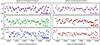 |
Fig. A.1. Residuals between the SED fitting results from J-PAS and SDSS surveys and their corresponding observed fluxes. The circles represent the residuals associated with the J-PAS data, while the triangles indicate those derived from SDSS. The color coding of the J-PAS data matches that of the polygons shown in Fig. 1, ensuring consistency across the figures and facilitating visual comparison. The data used to generate these residual plots are available on Zenodo; further details can be found in Appendix E.7. |
Appendix B: CIGALE configuration for SED fitting
The main grid parameters modified in the CIGALE configuration file are listed below. For further details, the complete configuration file is available on Zenodo.
tau_main = 50.0,  100.0, 500.0, 1000.0
age_main = 500.,  1000., 2000., 3000., 4000.,
           4025., 4050., 4075., 4100., 4125.,
           4150., 4175., 4200., 4225., 4250.,
           4275., 4300., 4325., 4350., 4375.,
           4400., 4425., 4450., 4475., 4500.,
           4525., 4550., 4575., 4600., 4625.,
           4650., 4675., 4700., 4725., 4750.,
           4775., 4800., 4825., 4850., 4875.,
           4900., 4925., 4950., 4975., 5000.,
           5025., 5050., 5075., 5100., 5125.,
           5150., 5175., 5200., 5225., 5250.,
           5275., 5300., 5325., 5350., 5375.,
           5400., 5425., 5450., 5475., 5500.
tau_burst   = 1.0, 5.0, 20.0, 50.0, 100.0
age_burst   = 10., 100., 500.
f_burst     = 0.001, 0.005, 0.01, 0.2
metallicity = 0.0001, 0.0004, 0.004, 0.008,
              0.02, 0.05
E_BV_lines  = 0.0, 0.1, 0.2, 0.3, 0.5, 0.7,
              0.8
E_BV_factor = 0.44
sfr_A       = 1.0
Appendix C: CIGALE using the Salpeter IMF
To compare the stellar mass obtained from the SED fitting with B03, we ran CIGALE using the Salpeter (1955) IMF. This choice was necessary because B03 employed the Salpeter (1955) IMF in their M/L relation. It is therefore essential to check how the different IMF we used in the main CIGALE SED fitting affects our result. For this reason, we executed CIGALE with exactly the same grid parameters described in Appendix B, but substituting the Salpeter (1955) IMF. The resulting parameter values are presented in the corner plot of Fig D.1.
As shown in Fig D.1 and 5, the stellar mass derived with the Salpeter (1955) IMF is larger than that obtained with the Chabrier (2003) IMF. This difference may be explained by the underlying assumptions of the two models. Specifically, the Salpeter (1955) IMF accounts for a greater number of low-mass stars compared to the Chabrier (2003) IMF, which leads to systematically higher stellar mass estimates.
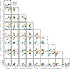 |
Fig. C.1. Corner plot of CIGALE output properties for J-PAS (in cyan) and SDSS data (in orange). In this run, the Salpeter (1955) IMF was used, and the main grid parameters modified in CIGALE were the same as those described in Appendix B. This step was taken because it is essential to ensure that the IMF applied in the CIGALE fitting is consistent with the IMF assumed in the M/L relations adopted by B03. The data used to generate this figure are available on Zenodo (see Appendix E.8). |
Appendix D: CIGALE excluding starburst
Because we observed many emission lines in the SED fitting derived from some of the polygons with SDSS fluxes (compared with those from J-PAS in Fig. 4), and since Alba no longer shows signs of strong star formation, we decided to disable all starburst components and nebular emission in the CIGALE configuration file to see their effect on the parameters discussed here. The resulting output properties are presented in the corner plot of Fig. D.1.
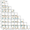 |
Fig. D.1. The corner plot of the CIGALE output properties for J-PAS (cyan) and SDSS (orange). In this analysis, both starburst and nebular components were excluded in order to isolate the underlying stellar population and reduce possible contamination in the derived parameters. The Chabrier (2003) IMF was adopted, and the complete set of modified grid parameters used in this run is provided in Appendix D. The dataset used to produce this figure is publicly available on Zenodo; further details are provided in Appendix E.9. |
By comparing Fig. D.1 (without starburst components) with Fig. 5 (with starburst components), it is evident that the J-PAS results change significantly. This is due to its higher resolution and larger number of filters: producing significantly different fits when the conditions change so drastically. Whereas the SDSS results remain largely unaffected after the omission of the starburst components, likely because of its lower resolution.
The main grid parameters used without the starburst components in the CIGALE configuration file are listed below. For additional details, the complete configuration file is available on Zenodo.
tau_main = 50.0,  100.0, 500.0, 1000.0
age_main = 10.,   100.,  500.,  1000., 2000.,
           3000., 4000.,
           4025., 4050., 4075., 4100., 4125.,
           4150., 4175., 4200., 4225., 4250.,
           4275., 4300., 4325., 4350., 4375.,
           4400., 4425., 4450., 4475., 4500.,
           4525., 4550., 4575., 4600., 4625.,
           4650., 4675., 4700., 4725., 4750.,
           4775., 4800., 4825., 4850., 4875.,
           4900., 4925., 4950., 4975., 5000.,
           5025., 5050., 5075., 5100., 5125.,
           5150., 5175., 5200., 5225., 5250.,
           5275., 5300., 5325., 5350., 5375.,
           5400., 5425., 5450., 5475., 5500.
tau_burst   = 1.0
age_burst   = 10.
f_burst     = 0
metallicity = 0.0001, 0.0004, 0.004, 0.008,
              0.02, 0.05
E_BV_lines  = 0.0, 0.1, 0.2, 0.3, 0.5, 0.7,
              0.8
E_BV_factor = 0.44
sfr_A       = 1.0
Figure Fig. D.2 is identical to Fig. 5, except for the ranges of the X and Y axes. To facilitate a clear comparison between Figs. D.1, C.1, and D.2, all figures have been plotted using the same axis ranges.
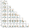 |
Fig. D.2. Same as Fig. 5, except for the ranges of the axes, which are the same as Figs. D.1 and C.1. |
Appendix E: figure and table data
This section provides links to the archived files of this project on zenodo.17674805. It contains all project source files to reproduce this analysis, as well as all the output tables behind every image and table in the PDF version.
E.1. Polygon coordinates (Fig. 1)
The coordinates of the polygons shown in Fig. 1 are provided in separate files: North-1 (polygon-1.reg), North-2 (polygon-2.reg), South (polygon-3.reg), East (polygon-4.reg), West-1 (polygon-5.reg), and West-2 (polygon-6.reg).
E.2. Data used to generate Fig. 2
The datasets used to generate the plot in Fig. 2 are available in the following files. The gray line corresponds to manga.txt. The orange circles in the upper panel correspond to jpas.txt, while the teal triangles in the upper panel correspond to sdss.txt. The black line is provided in manga-smooth.txt. The orange line corresponds to cigale-sed-fitting-center-jpas.txt, and the teal line corresponds to cigale-sed-fitting-center-sdss.txt. In the lower panel, the gray circles correspond to diff-manga-jpas.txt, the teal triangles correspond to diff-obs-sed-sdss.txt, and the orange circles correspond to diff-obs-sed-jpas.txt.
E.3. Surface brightness data for Fig. 3
The data used to generate the Fig. 3 can be accessed in the following files. Surface brightness data expressed in wavelength flux density units are provided for the following regions: North-1 (polygon-1-flux-density.txt), North-2 (polygon-2-flux-density.txt), South (polygon-3-flux-density.txt), East (polygon-4-flux-density.txt), West-1 (polygon-5-flux-density.txt), West-2 (polygon-6-flux-density.txt). Similarly, the surface brightness measurements expressed in AB magnitude units are available for the same regions: North-1 (polygon-1-sb.txt), North-2 (polygon-2-sb.txt), South (polygon-3-sb.txt), East (polygon-4-sb.txt), West-1 (polygon-5-sb.txt), West-2 (polygon-6-sb.txt).
E.4. SED fitting data for Fig. 4
The data required to reproduce the plots shown in Fig. 4 are available in following files. The dark purple circles and lines corresponding to the North-1 region are provided in the files north1-jpas.txt and north1-cgal-jpas.txt, respectively. The light purple circles and lines associated with North-2 are available in north2-jpas.txt and north2-cgal-jpas.txt. Similarly, the blue circles and lines representing the South region are contained in south-jpas.txt and south-cgal-jpas.txt. For the East region, the green circles and lines are provided in east-jpas.txt and east-cgal-jpas.txt, while the red circles and lines corresponding to West-1 are available in west1-jpas.txt and west1-cgal-jpas.txt. The peach-colored circles and lines associated with West-2 can be found in west2-jpas.txt, west2-cgal-jpas.txt. In addition, the gray triangles and lines derived from the SDSS data are distributed as follows: North-1 (north1-sdss.txt, north1-cgal-sdss.txt), North-2 (north2-sdss.txt, north2-cgal-sdss.txt), South (south-sdss.txt, south-cgal-sdss.txt), East (east-sdss.txt, east-cgal-sdss.txt), West-1: (west1-sdss.txt, west1-cgal-sdss.txt), and West-2 (west2-sdss.txt, west2-cgal-sdss.txt).
E.5. Data for tables 1 and 2
The underlying data for Tables 1 and 2 are available in the files table.tex and criteria.tex, respectively.
E.6. Corner plot data (Fig. 5)
The data used to generate the corner plot in Fig. 5 are available in the following files. The orange circles, corresponding to the J-PAS data, are provided in jpas-corner-plot.txt, while the teal circles, representing the SDSS data, are available in sdss-corner-plot.txt.
E.7. Residual plot data (Fig. A.1)
The data required to reproduce the plots shown in Fig. A.1 are available in the following files. For North-1, the dark violet data corresponding to J-PAS are provided in north1-residual-jpas.txt, while the gray teal data corresponding to SDSS can be found in north1-residual-sdss.txt. For North-2, the light violet data corresponding to J-PAS are available in north2-residual-jpas.txt, and the gray teal data corresponding to SDSS are provided in north2-residual-sdss.txt. For the South region, the blue data corresponding to J-PAS are available in south-residual-jpas.txt, while the gray teal data corresponding to SDSS can be found in south-residual-sdss.txt. For East, the green data corresponding to J-PAS are available in east-residual-jpas.txt, with the gray teal data corresponding to SDSS provided in east-residual-sdss.txt. For West-1, the red data corresponding to J-PAS are available in west1-residual-jpas.txt, while the gray teal data corresponding to SDSS can be found in west1-residual-sdss.txt. Finally, for West-2, the peach-colored data corresponding to J-PAS are available in west2-residual-jpas.txt, and the gray teal data corresponding to SDSS are provided in west2-residual-sdss.txt.
E.8. Corner plot data (Salpeter 1955 IMF, Fig. C.1)
The datasets used to produce the corner plot shown in Fig. C.1 with the Salpeter (1955) IMF are available in separate files. The orange circles correspond to the J-PAS data and can be accessed in jpas-salpiter.txt, whereas the teal circles represent the SDSS data and are available in sdss-salpiter.txt.
E.9. Corner plot data (no starburst or nebular, Fig. D.1)
The datasets used to generate the corner plot in Fig. D.1, without starburst and nebular components, are provided in separate files. The orange circles, representing the J-PAS data, can be accessed in jpas-no-sfr.txt, while the teal circles, corresponding to the SDSS data, are available in sdss-no-sfr.txt
All Tables
All Figures
|
Fig. 1. Alba galaxy (PGC 3087775) and its major merger remnants. The main panel shows surface brightness image of the Alba galaxy that is produced by co-adding all 57 J-PAS bands (including 54 narrowband filters, two medium-band filters, and one broadband filter; however, only the 56 narrow and medium-band filters are used in the analysis presented in this paper). The co-add reaches a 3σ mSBL over 100 arcsec2 of 29 mag/arcsec2. The color bar represents the surface brightness of the co-added image. The hexagon over the center of the galaxy delineates the MaNGA footprint used to validate J-PAS SEDs in Fig. 2. The six polygons delineated with the thin lines, are named and studied independently in subsequent figures (with the same color-coding). The lower left panel displays a false-color image from the HSC-SSP (Subaru) wide survey, created using the z, r, and g filters as the red, green, and blue. Polygon coordinates are on Zenodo (see Appendix E.1). |
| In the text | |
|
Fig. 2. Validation of J-PAS SEDs using MaNGA spectroscopy in the central region of the Alba galaxy (shown in Fig. 1). Top: Gray line indicates the MaNGA spectrum in this area, and the black line shows it after down-sampling with J-PAS filter throughputs. The orange points correspond to the measured J-PAS SED, and the solid orange line illustrates the best-fitting SED model derived from J-PAS data in the same region (after applying a minor constant correction factor of ×1.09 to all filters). Similarly, the teal triangles indicate the measured SDSS SED, and the solid teal line shows the corresponding SDSS SED fit (following the application of a small constant correction factor of ×0.96 to all filters). Some spectral line positions at the Alba galaxy redshift are also shown. Bottom: Percentage difference between the down-sampled MaNGA spectra and the J-PAS photometric data. This validates the very good calibration of J-PAS and allowed us to study regions beyond the small footprint of MaNGA. Furthermore, the orange and teal points and triangles represent the residuals between the SED fits derived from J-PAS and SDSS, respectively, and their corresponding observed fluxes. The dataset used to produce this plot can be accessed at Zenodo (see Appendix E.2). |
| In the text | |
|
Fig. 3. SED (in surface brightness) of different sections of the tidal feature, presented in two units. The top panel features units of wavelength flux density (used in the IFU community) of the six distinct polygons, while the lower panel features units of AB magnitude (used in the imaging community). The colors in this plot correspond to those used in Fig. 1 to represent different polygons. The gray bars at the bottom of each plot show the 3σ mSBL for each filter over an area of 100 arcsec2. The data used to generate this plot are available on Zenodo (see Appendix E.3). |
| In the text | |
|
Fig. 4. SED fitting on Alba’s tidal features. The measured SEDs and fitted spectra of the left and right panels show the inputs and outputs of CIGALE for both J-PAS and SDSS. They correspond to the named polygons of Fig. 1 with the same color. Circles show fluxes from 56 narrow/medium-band J-PAS filters, while triangles represent SDSS’s five broad filters. Fitted CIGALE spectra are overlaid using gray (SDSS) and colored (J-PAS) lines. The residuals between the SED fitting results of both surveys and their respective observed fluxes are presented in Appendix. A (Fig. A.1). The dataset underlying this plot is publicly accessible through Zenodo (see Appendix E.4). |
| In the text | |
|
Fig. 5. Corner plot showing the pairwise comparison of SED fitting output properties for J-PAS (teal circles) and SDSS (orange circles). In this analysis, all starburst and nebular components are included, and the Chabrier (2003) IMF is applied. Details of the grid parameters are provided in Appendix B. The 2D plots in the top right illustrate the comparison between J-PAS and SDSS in terms of the Dn(4000) index and stellar mass distribution. In addition, the stellar mass derived from SED fitting (from J-PAS and SDSS) is compared using the two following methods: Bell et al. (2003, labeled as B03) and García-Benito et al. (2019, labeled as GB19), both are based on the M/L ratio. The data used to generate this corner plot for both datasets are available on Zenodo (for further details, see Appendix E.6). |
| In the text | |
|
Fig. A.1. Residuals between the SED fitting results from J-PAS and SDSS surveys and their corresponding observed fluxes. The circles represent the residuals associated with the J-PAS data, while the triangles indicate those derived from SDSS. The color coding of the J-PAS data matches that of the polygons shown in Fig. 1, ensuring consistency across the figures and facilitating visual comparison. The data used to generate these residual plots are available on Zenodo; further details can be found in Appendix E.7. |
| In the text | |
|
Fig. C.1. Corner plot of CIGALE output properties for J-PAS (in cyan) and SDSS data (in orange). In this run, the Salpeter (1955) IMF was used, and the main grid parameters modified in CIGALE were the same as those described in Appendix B. This step was taken because it is essential to ensure that the IMF applied in the CIGALE fitting is consistent with the IMF assumed in the M/L relations adopted by B03. The data used to generate this figure are available on Zenodo (see Appendix E.8). |
| In the text | |
|
Fig. D.1. The corner plot of the CIGALE output properties for J-PAS (cyan) and SDSS (orange). In this analysis, both starburst and nebular components were excluded in order to isolate the underlying stellar population and reduce possible contamination in the derived parameters. The Chabrier (2003) IMF was adopted, and the complete set of modified grid parameters used in this run is provided in Appendix D. The dataset used to produce this figure is publicly available on Zenodo; further details are provided in Appendix E.9. |
| In the text | |
|
Fig. D.2. Same as Fig. 5, except for the ranges of the axes, which are the same as Figs. D.1 and C.1. |
| In the text | |
Current usage metrics show cumulative count of Article Views (full-text article views including HTML views, PDF and ePub downloads, according to the available data) and Abstracts Views on Vision4Press platform.
Data correspond to usage on the plateform after 2015. The current usage metrics is available 48-96 hours after online publication and is updated daily on week days.
Initial download of the metrics may take a while.