| Issue |
A&A
Volume 709, May 2026
|
|
|---|---|---|
| Article Number | A56 | |
| Number of page(s) | 19 | |
| Section | Stellar atmospheres | |
| DOI | https://doi.org/10.1051/0004-6361/202558421 | |
| Published online | 05 May 2026 | |
Clouds with a silicate lining: Using JWST spectra to probe atmospheric diversity in young AB Dor L dwarfs
1
School of Physics, Trinity College Dublin, The University of Dublin,
Dublin 2,
Ireland
2
Department of Astrophysics, American Museum of Natural History,
Central Park West at 79th St,
New York,
NY
10024,
USA
3
Center for Interdisciplinary Exploration and Research in Astrophysics (CIERA), Northwestern University,
1800 Sherman,
Evanston,
IL
60201,
USA
4
School of Physical Sciences, The Open University,
Milton Keynes,
MK7 6AA,
UK
5
Planétarium de Montréal, Espace pour la Vie,
4801 av. Pierre-de Coubertin, Montréal,
Québec,
Canada
6
Trottier Institute for Research on Exoplanets, Université de Montréal, Département de Physique,
C.P. 6128 Succ. Centre-ville,
Montréal,
QC
H3C 3J7,
Canada
7
Department of Physics & Astronomy, Amherst College,
25 East Dr.,
Amherst,
MA
01002,
USA
8
Institute for Astronomy, University of Edinburgh, Royal Observatory,
Edinburgh
EH9 3HJ,
UK
9
Centre for Astrophysics Research, Department of Physics, Astronomy and Mathematics, University of Hertfordshire,
Hatfield
AL10 9AB,
UK
10
Department of Physics and Astronomy, Hunter College, City University of New York,
695 Park Avenue,
New York,
NY
10065,
USA
11
Department of Astronomy, University of Texas at Austin,
2515 Speedway,
Austin,
TX
78712,
USA
12
New York University,
New York,
NY
10003,
USA
13
Department of Astronomy, Columbia University,
550 West 120th Street,
New York,
NY
10027,
USA
14
Department of Astronomy & Astrophysics, University of California,
Santa Cruz,
CA
95064,
USA
15
Department of Physics, Graduate Center, City University of New York,
365 5th Avenue,
New York,
NY
10016,
USA
★ Corresponding author: This email address is being protected from spambots. You need JavaScript enabled to view it.
Received:
5
December
2025
Accepted:
25
March
2026
Abstract
Aims. We present the first full JWST NIRSpec Prism and MIRI LRS 0.6–14 μm (R ~ 100) spectra and analysis of five ~133 Myr L dwarf members of the AB Doradus moving group and one probable ~500 Myr T dwarf of the Oceanus moving group with known inclination angles between ~23–90°: 2MASS J00470038+6803543, 2MASS J03552337+1133437, 2MASS J06420559+4101599, 2MASS J17410280–4642218, 2MASSW J2206450–421721, and 2MASS J22443167+2043433.
Methods. We constructed near-complete spectral energy distributions of each of our objects to measure their bolometric luminosities, and we estimated their fundamental parameters (Teff, radius, M, and log g). We used cross-sections of relevant gases to identify the species that are present in each atmosphere. Of particular interest is the silicate absorption feature at 8–11 μm, which provides insight into the complex cloud structure of brown dwarfs. We examined this silicate absorption feature in detail and tested whether a latitudinal dependence exists in the silicate absorption feature within a coeval sample of brown dwarfs.
Results. Various molecular absorption bands are visible in our spectra, including H2O, CH4, CO, and CO2. The shape of the silicate absorption feature varies within our sample, and we find that four out of five of our L type objects agree with previously observed trends, namely, that objects viewed equator-on have deeper silicate absorption. We highlight W1741–46 as an outlier in our sample with an unusually strong silicate absorption given its near pole-on orientation. We also present a tentative correlation between the wavelength of peak silicate absorption and inclination, which may suggest variations in cloud chemical composition or physical properties.
Conclusions. We found an unexpected spectral diversity within our sample, which motivates future studies on these objects through atmospheric retrievals, which will determine the silicate cloud composition and reveal whether there exists a trend with inclination.
Key words: planets and satellites: atmospheres / brown dwarfs
© The Authors 2026
 Open Access article, published by EDP Sciences, under the terms of the Creative Commons Attribution License (https://creativecommons.org/licenses/by/4.0), which permits unrestricted use, distribution, and reproduction in any medium, provided the original work is properly cited.
This article is published in open access under the Subscribe to Open model. This email address is being protected from spambots. You need JavaScript enabled to view it. to support open access publication.
1 Introduction
Brown dwarfs are substellar objects that exist in the intermediate mass range (M ~ 13–78.5 MJup; Kumar 1963; Chabrier et al. 2023) between stars and planets. Brown dwarfs cool over time, reaching temperatures that rival Solar System objects or the coldest directly imaged exoplanets, for example WISE 0855–0714 at 250 K (Luhman 2014), Eps Ind Ab at 275 K (Matthews et al. 2024), and 14 Her c at 250–300 K (Bardalez Gagliuffi et al. 2021, 2025). They can be considered ‘overachieving planets’, as they are similar to giant planets in terms of their temperature, composition, and radius (Burrows et al. 2001), but they tend to be more massive. Direct imaging of exoplanet atmospheres is challenging due to their bright host star drowning out the light emitted from the exoplanet itself. However, brown dwarfs provide an alternative route to study extrasolar atmospheres, as they are often found in isolation, alleviating the problem of blocking a bright host star. As a result, we have a larger sample of brown dwarfs and higher quality observations compared to exoplanets. Studying brown dwarfs in the context of planetary atmospheres will allow us to better understand exoplanet atmospheric processes and dynamics (Apai et al. 2017; Showman et al. 2020).
Over time, brown dwarfs cool and evolve across the L-T-Y spectral types and change their infrared (IR) colours, which reflects changes in their temperature and atmospheric chemical composition. Brown dwarfs of the L spectral type have effective temperatures (Teff) similar to many directly imaged exoplanets (e.g. HR 8799 bcde; Marois et al. 2008, 2010). Thus, L dwarfs can be used as proxies for gas giants. L dwarfs are defined by the strengthening of neutral alkali lines, oxides, and hydrides in their spectra, which can be translated into effective temperatures between 1300–2500 K (Kirkpatrick 2005). L dwarfs are of particular interest as silicate clouds condense in the photosphere, making these brown dwarfs appear redder in the near-infrared (NIR) compared to other spectral types (e.g. Ackerman & Marley 2001; Marley et al. 2002; Tsuji 2002; Knapp et al. 2004; Burrows et al. 2006; Cushing et al. 2006; Marley et al. 2010). At the L-T spectral transition (~1000–1200 K for low gravity objects with log g ~ 4–4.5), the influence of silicate clouds on the spectral morphology reduces, shifting the NIR colours of these brown dwarfs to bluer wavelengths (Ackerman & Marley 2001; Saumon & Marley 2008). Alternative theories suggest that the brightening of the J-band for L dwarfs close to the L-T transition is not caused by silicate clouds but instead by energy transport from non-equilibrium carbon chemistry (Tremblin et al. 2016). These silicate clouds are thought to be one of the primary drivers of variability observed on L dwarfs in IR wavelengths (e.g. Artigau et al. 2009; Radigan et al. 2012; Apai et al. 2013; Lew et al. 2016; Vos et al. 2020; Suárez & Metchev 2022; Vos et al. 2022). Studying cloud variability in brown dwarfs provides an enhanced insight into the atmospheric dynamics of extrasolar gas giant planets with similar fundamental properties (e.g. Ge et al. 2019; Bowler et al. 2020; Gao et al. 2021).
Silicate clouds in L dwarfs are thought to be produced by Si- and Mg-chemistry forming three main compositions (Lodders & Fegley 2002): enstatite (MgSiO3), forsterite (Mg2SiO4), and quartz (SiO2), which shape the silicate absorption feature present at mid-IR wavelengths (Luna & Morley 2021). This silicate absorption at 8–11 μm caused by Si-O bonds stretching has been observed in many brown dwarfs by the Spitzer Infrared Spectrograph (IRS; Cushing et al. 2006; Stephens et al. 2009; Suárez & Metchev 2022). The silicate absorption feature has also been detected in brown dwarfs and directly imaged exoplanets with the Mid-Infrared Instrument (MIRI) on the James Webb Space Telescope (JWST; e.g. Miles et al. 2023; Biller et al. 2024; Chen et al. 2025; Hoch et al. 2025; Mollière et al. 2025). The shape of the silicate feature (peak wavelength, width, depth) provides insight into the silicate composition and grain size (Luna & Morley 2021; Suárez & Metchev 2023). Atmospheric retrieval, a data-driven modelling technique, has been used to disentangle the cloudy structure of brown dwarf atmospheres, revealing structures such as patchy Mg2SiO4 clouds (Vos et al. 2023) or layers of MgSiO3 and SiO2 (Burningham et al. 2021), supporting the hypothesis that clouds drive the variability observed in brown dwarfs. Recently, SiO2 clouds have also been observed in the atmospheres of transiting hot Jupiter exoplanets (Grant et al. 2023) with JWST/MIRI.
The inclination angle, i, has emerged in recent years as an important property of an observed atmosphere. Notably, brown dwarfs that are viewed equator-on appear both redder and more variable than those viewed pole-on (Vos et al. 2017, 2018, 2020). We define the inclination angle to be the viewing angle relative to the object’s equator from our line of sight. To calculate the inclination angle of an object, we require high-resolution spectra in order to measure the projected rotational velocity, v sin i. Combined with the radius from fitting evolutionary models and the rotational period obtained from variability studies, we can calculate the inclination angle. Suárez et al. (2023) also observed that the mid-IR silicate absorption feature was more prominent for brown dwarfs observed closer to equator-on. Thus, we can interpret that objects viewed equator-on appear redder and more variable due to the varying temperature or particle size of silicate cloud layers. Higher altitude clouds are expected to be redder because they are cooler than clouds deeper in the atmosphere (Ackerman & Marley 2001). This latitudinal variation in cloud thickness has also been theoretically predicted by general circulation model (GCM) simulations (Showman et al. 2020; Tan & Showman 2021). The polar vortex hypothesis (Fuda & Apai 2024), for example, explains how jet-dominated bands across the equator and vortex-dominated poles could cause similar observed variations. However, different ages or overall chemical compositions in previously studied samples could cause these latitudinal differences. In this work, we study the silicate feature for a sample of coeval objects for the first time, and we investigate the hypothesis that atmospheric dynamics in L dwarfs drive equator-to-pole differences in cloud properties.
In this paper we present the first analyses of JWST spectra of a sample of ~133 Myr AB Doradus moving group (hereafter, AB Dor) objects. Section 2 describes relevant properties of our sample of AB Dor members. In Sect. 3, we discuss the observations and data reduction of our JWST spectra as well as the high-resolution spectra we obtained from IGRINS for v sin i measurements. In Sect. 4.1, we present new and updated spectral types for each of our objects based on our new spectra. In Sect. 4.2, we construct a full spectral energy distribution (SED) for each of our objects to measure the bolometric luminosity, effective temperature, mass, radius, and surface gravity. We also present new rotational and radial velocity (RV) measurements from the Immersion GRating INfrared Spectrometer (IGRINS) for two of the objects in our sample in Sect. 4.3. In Sect. 5, we highlight which molecules are present in the atmospheres of the objects in our sample and measure the water, methane, and silicate indices of each object. We also discuss whether we observe any trends between inclination and the silicate feature. In Sect. 6, we compare our JWST spectra to previous Spitzer observations to test for evidence of long-term variability and JWST spectra of other similar planetary mass objects from the literature.
2 Sample properties
Our sample comprises six well-characterised L dwarfs: 2MASS J00470038+6803543, 2MASS J03552337+1133437, 2MASS J06420559+4101599, 2MASS J17410280–4642218, 2MASSW J2206450–421721, and 2MASS J22443167+2043433 (hereafter W0047+68, 2M0355+11, 2M0642+41, W1741–46, 2M2206–42, and 2M2244+20, respectively). We have chosen these targets because all except one are bona fide (BF) members of the AB Dor moving group (see Table 1). Objects in the same moving group form together from the same molecular cloud, and hence have the same age and similar chemical composition. Therefore, studying low-temperature objects in the same moving group provides an ideal coeval sample of exoplanet analogues, where we can uniquely isolate effects due to effective temperature or inclination. All targets except 2M2206–42 have published variability detections and period measurements with Spitzer (Vos et al. 2018, 2022) and combined with their v sin i we can measure their inclinations. For 2M2206–42, we can estimate its inclination using the range of expected rotational periods for AB Dor objects. This makes our sample an ideal testbed for exploring potential trends with inclination. We also have the opportunity to characterise this unique sample in unprecedented detail with our high-quality observations.
Using the kinematic properties of our targets, including parallax (π), proper motion (μ), and RV, we calculated the membership probability for each target with the BANYAN Σ tool (Gagné et al. 2018b), and present them in Table 1. We use the membership definitions from Faherty et al. (2016) to describe our objects. BF members have full kinematic information (proper motions and radial velocities) and a high probability (>90%) of membership. Ambiguous members (AM) require more kinematic information because they could belong to more than one group. Since our sample are either BF or AM members of the young AB Dor moving group they are likely to be the same age (![Mathematical equation: $\[133_{-20}^{+15}\]$](/articles/aa/full_html/2026/05/aa58421-25/aa58421-25-eq4.png) Myr; Gagné et al. 2018a) and have similar metallicity.
Myr; Gagné et al. 2018a) and have similar metallicity.
2M0642+41 is the only AM member in our sample because it is missing an RV measurement, which could place it in the Oceanus moving group (~500 Myr) instead (Gagné et al. 2023). With the original BANYAN Σ models (Gagné et al. 2018b), we find a 74.4% membership probability in AB Dor, with an optimal RV of 0.2 ± 1.4 km/s. With newer models (Gagné et al. 2026), we get a higher membership probability in the Oceanus moving group with 88.2% and a predicted RV of 12.9 ± 0.9 km/s. Updated parallax and proper motion measurements from Best et al. (2024) favour the Oceanus moving group. However, we require a precise RV measurement for 2M0642+41 to determine which moving group it is a member of.
The location of each object on a NIR colour–magnitude diagram is shown in Fig. 1. We focused on the J and K bands to highlight previous observations of the unusually red colours of objects in our sample. Our objects span the L dwarf to L–T transition range and are redder than most L dwarfs, a key property of young objects (Faherty et al. 2016; Liu et al. 2016). These redder colours are caused by the presence of silicate clouds in the photosphere (e.g. Saumon & Marley 2008; Faherty et al. 2013; Best et al. 2015; Suárez & Metchev 2022). Our sample of brown dwarfs are comparable on the colour-magnitude diagram to VHS J125601.92-125723.9 b (hereafter VHS 1256 b; Gauza et al. 2015), a planetary-mass companion that was observed by the first JWST early-release science program (Miles et al. 2023), a planetary-mass object PSO J318.5338-22.8603 (hereafter PSO J318; Liu et al. 2013), and the HR 8799 planets (see our Fig. 1 and Marois et al. 2008, 2010). Thus, our sample of brown dwarfs provides critical context to interpret observations of directly imaged exoplanets.
Table 2 list parameters of interest (including rotational periods, variability amplitudes and inclination) of our sample. The following paragraphs elaborate on parameters for each object in our sample.
W0047+68 (Gizis et al. 2012, 2015) is an unusually red (J − Ks = 2.5 ± 0.1 mag; Best et al. 2021) dwarf with optical spectral type L7 γ and IR type L6-8 γ (Gizis et al. 2012, 2015). It has one of the highest known variable amplitudes observed with both the Hubble Space Telescope (HST; 11% at 1.1 μm; Lew et al. 2016) and the Spitzer Space Telescope (1.07 ± 0.04% at 3.6 μm) with a rotational period of 16.4 ± 0.2 h (Vos et al. 2018). It is viewed equator-on with a measured inclination of ![Mathematical equation: $\[i=85_{-9}^{+5^{\circ}}\]$](/articles/aa/full_html/2026/05/aa58421-25/aa58421-25-eq12.png) (Vos et al. 2018).
(Vos et al. 2018).
2M0355+11 (Reid et al. 2008) is an extremely red (J − Ks = 2.438 ± 0.004; Lawrence et al. 2007; Schneider et al. 2023) object with optical spectral type L5 γ (Cruz et al. 2009) and IR type L3-6 γ (Gagné et al. 2015). Significant variability (0.26 ± 0.02%) with a period of 9.53 ± 0.19 h was measured in the 3.6 μm band with Spitzer (Vos et al. 2022). Suárez et al. (2023) measured an inclination angle of i = 50 ± 2°.
2M0642+41 (Mace et al. 2013) was discovered as an ‘extremely red’ object in the H band and later classified as an IR L9 (Best et al. 2015). It is not as red in the NIR with J − Ks = 1.86 ± 0.02 mag (Schneider et al. 2023). It has the highest measured variability amplitude at 3.6 μm of 2.16 ± 0.16% with a period of 10.11 ± 0.06 h from Spitzer (Vos et al. 2022).
W1741–46 (Schneider et al. 2014) is an IR L6-8 γ (Gagné et al. 2015; Faherty et al. 2016) dwarf with a particularly red NIR colour of J − Ks = 2.56 ± 0.05 mag (McMahon et al. 2013; Best et al. 2021). It has detected variability with a low amplitude (0.35 ± 0.03% at 3.6 μm) with a period of ![Mathematical equation: $\[15.00_{-0.57}^{+0.71}\]$](/articles/aa/full_html/2026/05/aa58421-25/aa58421-25-eq13.png) h (Vos et al. 2022).
h (Vos et al. 2022).
2M2206–42 (Kirkpatrick et al. 2000) is an optical and IR L4 γ (Gagné et al. 2015; Faherty et al. 2016) dwarf. It is not particularly redder than other L dwarfs with similar magnitudes with J − Ks = 1.9 ± 0.1 mag (Best et al. 2021). It has a non-detection of variability from a Spitzer light curve at 3.6 μm (Vos et al. 2022).
2M2244+20 (Dahn et al. 2002) is a very red (J − Ks = 2.57 ± 0.02 mag Schneider et al. 2023) optical L6.5 (Allers & Liu 2013) and IR L6-8 γ (Faherty et al. 2016) object that is spectroscopically similar to W0047+68 (Gizis et al. 2015). Variability has been detected by Spitzer at 4.5 μm (Morales-Calderón et al. 2006) and more recently, at 3.6 μm with an amplitude of 0.8 ± 0.2% and rotational period of 11 ± 2 h (Vos et al. 2018). There has also been variability detected in the J-band light curve with an amplitude of 5.5% (Vos et al. 2019). This object has an inclination angle of ![Mathematical equation: $\[i=76_{-20}^{+14^{\circ}}\]$](/articles/aa/full_html/2026/05/aa58421-25/aa58421-25-eq14.png) (Vos et al. 2018).
(Vos et al. 2018).
Kinematic properties for objects in our sample.
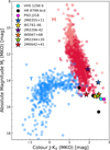 |
Fig. 1 Colour-magnitude diagram indicating locations of our targets (coloured stars) at the L-T transition. The location of VHS 1256 b has also been included as a cyan circle. Planets in the HR 8799 system are also indicated as black circles. PSO J318 is indicated as a pink circle. The coral points are M dwarfs, dark red points are L dwarfs, and blue points are T dwarfs. Photometric data for each point was obtained from the Ultracool Sheet (Best et al. 2024). |
Variability and inclination measurements for objects in our sample.
3 Observations and data reduction
3.1 JWST
We observed our six objects using JWST MIRI (Rieke et al. 2015) and the Near Infrared Spectrograph (NIRSpec; Jakobsen et al. 2022) instruments to obtain near-simultaneous R ~ 100 spectra from 0.6–14 μm (PI: Vos, GO 3486). The same detector setup was used for all targets. Only the exposure times varied according to the brightness of each target. A summary of the observations can be found in Table 3.
We used the MIRI Low Resolution Spectrometer (LRS) fixed-slit mode (4.7″ × 0.51″) to obtain 5–14 μm spectra with a resolving power varying from R ~ 40–160 for each target. We used the default P570L disperser and FULL sub-array with the FAST readout pattern. We also used the F1000W filter during target acquisition. We used the two-point along slit AB nod pattern to obtain two total dithers. The exposure time for each target (see Table 3) was calculated to ensure a S/N > 75 at 10 μm for all targets, so that the silicate feature at 8–11 μm can be robustly analysed.
During the same visit as our MIRI observations, we obtained NIRSpec spectra between 0.6–5.3 μm for the same target. NIRSpec was used in fixed-slit mode with the Prism/CLEAR grating/filter pair, the S200A1 slit (0.2″ × 3.2″), and the NRSRAPID readout pattern. This filter provided a spectral resolution of R ~ 100. We observed in an AB nod pattern with four total dithers. With the exposure times in Table 3, we achieved S/N >100 across the 1–5.2 μm wavelength range, which is sufficient to constrain atmospheric properties from the water, methane, and carbon monoxide features.
3.1.1 Data reduction
We used the JWST calibration pipeline version 1.16.0 (Bushouse et al. 2024) with CRDS context file jwst_1322.pmap to reduce the JWST data, starting from uncalibrated data downloaded from the Mikulski Archive for Space Telescopes (MAST). Default parameters were used when processing the spectra through each of the three stages.
Stage 1 of the pipeline applies detector-level corrections and ramp fitting to the uncalibrated ramp data for each exposure. This includes dark and bias subtraction, removal of bad pixels and cosmic ray detection, for example. This stage produces two-dimensional count rate images for each exposure. Stage 2 uses the uncalibrated slope images produced by stage 1 to perform instrument calibrations for each exposure. This includes pixel flat-fielding, flux calibration and assigning world coordinate information. This stage outputs calibrated slope images. Finally, Stage 3 combines each of the corrected dithers into a single science-ready spectrum. We use the final x1d.fits file in our data analysis throughout this paper. This was repeated for each object for both NIRSpec Prism and MIRI LRS to obtain a full 0.6–14 μm spectrum.
Summary of JWST observations.
3.1.2 Flux calibration and merging of spectra
To create a continuous 0.6–14 μm spectrum for each object, the NIRSpec Prism and MIRI LRS spectra were merged. At the overlap window of 5–5.3 μm, we monitored the S/N of the NIRSpec spectra. When the S/N first drops below a threshold of 80 within the 5–5.3 μm overlap region, we cut off the NIRSpec spectrum and switch to MIRI. This threshold was chosen to balance a high S/N with maintaining the higher spectral resolution provided by NIRSpec to resolve molecular features in this region, which would not be possible at this wavelength with MIRI LRS.
All objects except 2M2244+20 have consistent flux in the NIRSpec and MIRI overlap region, which is expected due to the near-simultaneous observations. However, 2M2244+20 has a flux offset between the NIRSpec and MIRI observations, where the NIRSpec spectrum has approximately 30% less flux than the MIRI spectrum within the overlap region. The NIRSpec exposure started 27.6 min after the start of the MIRI exposure. This large difference cannot be explained by the object’s variability (0.8% at 3.6 μm with P = 11.0 ± 2.0 h; Vos et al. 2018) or any other physical atmospheric processes. We also compared synthetic photometry calculated from our JWST spectra with literature photometric points obtained from MKO (Schneider et al. 2023) and WISE (Lang et al. 2016), which indicated that the NIRSpec spectrum had lower flux than expected. The flux from our MIRI spectrum matched well with literature photometry as well as archival Spitzer IRS spectra (Suárez & Metchev 2022). Thus, we determined that the offset was possibly due to a slit misalignment from imperfect NIRSpec target acquisition. Objects in our sample have high proper motions (see Table 1), which may have contributed to the difficulty of acquiring the target. The NIRSpec target acquisition field of view is smaller than that of MIRI (see Sect. 3.1), which may have led to the difficulty in acquisition. To circumvent this issue, we normalised the NIRSpec spectrum to the flux in the overlapping region with MIRI LRS to create a continuous, high S/N 0.6–14 μm spectrum.
After data reduction, we used SEDkit (Filippazzo et al. 2015) to normalise each spectra to 10 pc using the measured parallaxes from the literature (shown in Table 1). We present the combined NIRspec and MIRI spectra for all objects in our sample in Fig. 2.
3.2 High-resolution spectra
The IGRINS instrument is a high-resolution (R ~ 45 000) NIR spectrograph on Gemini South (Yuk et al. 2010; Park et al. 2014; Mace et al. 2016, 2018). IGRINS has two separate spectrograph arms to cover the H and K bands, resulting in full coverage of the wavelength range between 1.45–2.45 μm.
We obtained IGRINS spectra for the two objects with missing inclination measurements (PI: Vos, PID: GS-2020B-Q-246). W1741–46 was observed on three nights at UTC 2021-01-24 08:57:06, 2021-01-27 08:53:52, and 2021-01-28 08:57:37. All observations had an integration time of 350 s. The observation on 2021-01-24 had low S/N ~10 at and the observation on 2021-01-27 had S/N ~30, likely due to high air mass. The observation on 2021-01-28 had a S/N ~ 300 in the centre of the order of interest (77), so we used this night’s spectrum for our final results and analysis. 2M2206–42 was observed on UTC 2020-11-16 01:46:26 for an integration time of 200 s, resulting in a max S/N ~30 in the middle of order 77.
Reduced IGRINS spectra were downloaded using version 3 of the Raw and Reduced IGRINS Spectral Archive (RRISA; Kaplan et al. 2024; Sawczynec et al. 2025). The IGRINS Pipeline Package (Kaplan et al. 2024) removes effects due to cosmic rays, corrects for instrumental flexures, stacks individual exposures, removes sky emission features and the detector readout pattern, applies flat fielding, corrects individual echelle orders, calculates the wavelength solution, and extracts the flux per pixel and variance spectra.
A high-resolution Gemini Near-InfraRed Spectrograph spectrum for 2M0642+41 is also publicly available (PI: Best, PID: GN-2015B-FT-14). This spectrum was observed on UTC 2016-1-09. However, when analysing this spectrum, we noticed that the spectrum had a very low S/N, so we were unable to measure an accurate v sin i or RV. With better quality spectra of 2M0642+41, we would be able to both confirm its moving group membership, as well as measure its v sin i and inclination angle.
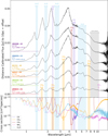 |
Fig. 2 Top panel: distance-calibrated spectra for each object. Shaded regions show key absorption bands for CH4, CO, CO2, NH3 and H2O. The dotted line shows the offset level for each spectrum. The spectra are ordered by decreasing effective temperature from top to bottom. Bottom panel: cross-sections for each species, computed at T = 1300 K and P = 1 bar. |
Fundamental parameters from SED analysis with updated spectral types for each object.
4 Spectral, fundamental, and kinematic parameters
4.1 Updated spectral typing
We reclassified the spectral types of the objects in our sample by comparing the recently obtained NIRSpec Prism spectra to field gravity (α), intermediate gravity (β) and very low gravity (γ) NIR spectral standards for L & T dwarfs (Bickle et al. in prep.). As there are variations in the NIR slope between our sample and the spectral standards, each object’s J-, H- and K-bands were individually de-reddened using the Cardelli et al. (1989) extinction law. For each band, E(B − V) (colour excess due to reddening) and RV (total-to-selective extinction ratio) values were adjusted until the best χ2 fit was achieved to the respective band of each standard, and the resulting fits were visually compared to determine the best spectral type match.
The benefit of this de-reddening approach versus simple band-by-band normalisation (e.g. Cruz et al. 2018) is that some objects can appear redder even within a spectral band (J, H or K), not just across bands, due to peculiar composition, clouds or youth. This is especially true near the L/T transition where field objects can show a wide range of slopes even within a single band, within one spectral subtype. This scheme therefore allows us to place objects more robustly on the grid of spectral standards and assess for peculiarities independent of slope changes. Interstellar extinction laws have previously been shown to improve the spectral fits of young brown dwarfs to model spectra (Petrus et al. 2020, 2024; Hurt et al. 2024; Mader et al. 2026), suggesting that they may indeed act as appropriate analogues for the extinction within young substellar atmospheres. Nonetheless, we treat the extinction parameters providing the best fits to our objects as nuisance parameters and not as physically relevant quantities.
The de-reddened NIRSpec Prism spectra for our sample are plotted against their respective best fitting spectral standard in Fig. 3 and we present our updated spectral types in Table 4. The adopted spectral types in Table 4 do not necessarily match the best fitting spectral standards presented in Fig. 3, as the fits of some objects are in between multiple spectral standards, which results in a range of spectral types in Table 4.
Of significant note is 2M0642+41, which was previously classified as L9 (Best et al. 2015) but has been confirmed to be a T1 object instead. Figure 4 shows its NIRSpec spectrum de-reddened and compared to L8-T2γ spectral standards. Note that the overall continuum shape and, crucially, the CH4 absorption bands which define the transition into the T dwarfs (Burgasser et al. 2002), are best fit to the T1γ standard. Our updated spectral classification of 2M0642+41 as T1 is supported by its bluer position on the colour-magnitude diagram (see Fig. 1).
The absence of the mid-IR silicate absorption feature in 2M0642+41 is consistent with its updated spectral classification. At the L/T transition, silicate clouds sink below the photosphere (Ackerman & Marley 2001; Saumon & Marley 2008; Cushing et al. 2006; Suárez et al. 2021a).
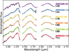 |
Fig. 3 JWST/NIRSpec Prism spectra of our sample (coloured) compared to their respective best-fitting spectral standard (black) after de-reddening (Bickle et al., in prep.). |
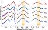 |
Fig. 4 JWST/NIRSpec Prism NIR spectrum of 2M0642+41 (black) de-reddened and compared to L/T transition low-gravity spectral standards. The T1γ spectral standard is the best fit to 2M0642+41. The CH4 absorption regions are shaded in orange. |
4.2 Fundamental parameters
Spectral energy distributions can be used to determine bolometric luminosities (Lbol) and combined with age estimates and evolutionary models, we can estimate the fundamental parameters, i.e. effective temperature (Teff), radius, mass (M) and surface gravity (log g), of brown dwarfs (e.g. Filippazzo et al. 2015; Best et al. 2021; Kirkpatrick et al. 2021). These parameters further characterise our sample and place them in context with a wider sample of brown dwarfs. Physical parameters derived from the bolometric luminosity and ages from SEDs depend on evolutionary models, rather than atmospheric models, which can have systematic uncertainties introduced from their sensitivity to boundary conditions (Filippazzo et al. 2015; Suárez et al. 2021b; Sanghi et al. 2023).
We constructed entire SEDs for each object in our sample by combining our 0.6–14 μm spectra and existing photometric points from 2MASS and WISE. We used SEDkit (Filippazzo et al. 2015) to interpolate the Saumon & Marley (2008) evolutionary model to the SEDs to obtain their fundamental parameters. The Lbol for each object was calculated by integrating under the flux-calibrated SEDs. SEDkit then uses the Lbol and the object’s age (![Mathematical equation: $\[133_{-20}^{+15}\]$](/articles/aa/full_html/2026/05/aa58421-25/aa58421-25-eq18.png) Myr for AB Dor members; Gagné et al. 2018a) to estimate the radius and M from the Saumon & Marley (2008) evolutionary model isochrones. Since 2M0642+41 is likely a member of the Oceanus moving group (see Sect. 2), we use the age of this moving group (510 ± 95 Myr; Gagné et al. 2023) to calculate the fundamental parameters instead. Teff was calculated by combining the radius and Lbol with the Stefan-Boltzmann law. Our measured values for each object are presented in Table 4.
Myr for AB Dor members; Gagné et al. 2018a) to estimate the radius and M from the Saumon & Marley (2008) evolutionary model isochrones. Since 2M0642+41 is likely a member of the Oceanus moving group (see Sect. 2), we use the age of this moving group (510 ± 95 Myr; Gagné et al. 2023) to calculate the fundamental parameters instead. Teff was calculated by combining the radius and Lbol with the Stefan-Boltzmann law. Our measured values for each object are presented in Table 4.
We have high quality JWST spectra covering the wavelength range between 0.6–14 μm, so we can construct the best possible SEDs for these objects and thus calculate the most precise measurements for the fundamental parameters. We calculated our SEDs to be >98% complete by comparing our SED to Sonora Diamondback models (Morley et al. 2024) using the SEDA (Spectral Energy Distribution Analyzer) package (Suárez et al. 2021b, Suárez et al., in prep.). Our measured Teff, radii, and M (see Table 4) are consistent with previously measured values from Filippazzo et al. (2015); Vos et al. (2022).
At ~ 133 Myr, W0047+68 and 2M2244+20 are close to the deuterium burning limit of ~12 − 13 MJup, meaning that we expect a bimodal distribution of masses, similar to VHS 1256 b (Miles et al. 2023; Dupuy et al. 2023). We implemented a similar rejection sampling method to Miles et al. (2023) with our Lbol to obtain a more robust measurement of the fundamental parameters for W0047+68 and 2M2244+20. We include the histograms for our posteriors in Appendix A.
In Fig. 5, we compare the Teff and M of our sample to a larger sample (>1000) of ultracool dwarfs, including older field dwarfs from Sanghi et al. (2023). Sanghi et al. (2023) measured their Lbol by integrating optical to mid-IR SEDs and used the Baraffe et al. (2015) and Saumon & Marley (2008) evolutionary models to determine the fundamental parameters for their sample. We notice that there is a large spread in our sample of brown dwarfs. Objects with a later spectral type have a cooler Teff, which agrees with the general trend observed from Sanghi et al. (2023). More massive brown dwarfs are hotter than those of the same spectral type. Younger objects also tend to have lower Teff compared to older field objects of the same spectral type (see the polynomial relation for young objects in our Fig. 5; Faherty et al. 2016; Sanghi et al. 2023). Most of our objects tend to follow the trend for young objects, apart from W1741–46, which appears to be closer to the old field relation, despite being a bona fide AB Dor member.
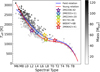 |
Fig. 5 Visualisation of the fundamental parameters of the sample analysed in Sanghi et al. (2023, grey circles) and our sample (coloured outlined stars). We note that Teff is plotted against the IR spectral type. The fill colour is indicative of the mass of the object. Random noise of 0.3 spectral types was added along the x-axis to minimise overlapping points in visualisation. The fundamental parameters were calculated using evolutionary models. The polynomial relations for the old field dwarfs and young moving group members (blue and red lines, respectively) from Sanghi et al. (2023) are overplotted. |
4.3 Rotational velocities
Previous studies have shown that there is a strong latitudinal dependence of clouds and infrared colours, where objects viewed equator-on appear redder than those viewed pole-on (Vos et al. 2017, 2020; Suárez & Metchev 2022; Suárez et al. 2023). This colour variation is believed to be caused by a larger vertical extent of clouds along the equator compared to the poles (Tan & Showman 2021). The larger vertical extent would lead to higher clouds at the equator, which are expected to be cooler and composed of smaller particles (Ackerman & Marley 2001). We aim to test this latitudinal dependence in our sample of young, coeval AB Dor members, removing any potential biases due to age. We have previous measurements for variability and inclination for four targets (W0047+68, 2M0355+11, 2M0642+41, and 2M2244+20; see Table 2). We used our high-resolution IGRINS spectra for the remaining two targets W1741–46 and 2M2206–42 to measure their v sin i, which is needed to determine their inclinations.
We used the Spectral Modelling Analysis and RV Tool (SMART; Hsu et al. 2021) to measure the v sin i for our remaining targets. SMART is a Markov chain Monte Carlo (MCMC) tool that can be used for high-resolution near-infrared spectra, including IGRINS. SMART uses a forward modelling method to simultaneously fit the wavelength solution, telluric line depths and the full width half maximum (FWHM) of the instrumental line spread function (LSF) of the standard star, and then uses this best-fit model with atmospheric models on the observed spectra to fit the free parameters for our target which include Teff, log g, v sin i, and RV.
We ran SMART on order 77 of the K-band spectrum. This order contains many CO absorption lines located in the wavelength range 2.293–2.325 μm. We chose to use the PHOENIX BT-Settl model atmosphere (Allard et al. 2012) to fit our spectra. We used 50 walkers and ran the MCMC for 600 burn-in steps. For 2M2206–42, we ran the MCMC for 600 steps, and for W1741–46, we increased it to 1200 to ensure that the walkers had converged by visually inspecting the trace and ensuring the output results were not changing significantly. We fit the L dwarf parameters Teff, log g, v sin i, and RV, as well as the parameters for instrumental or environmental effects: air mass, precipitable water vapour (pwv), flux offset (CFλ), wavelength offset (Cλ), and the noise factor (Cnoise). We set our prior ranges based on typical values for our L dwarf sample, with Teff = 1000–2000 K, log g = 4–5, v sin i = 0–50 km/s, and RV = −50–50 km/s. We present our new v sin i measurements in Table 2 and our final fits to the spectra in Fig. 6.
The fitted Teff and log g are less accurate than those determined from our earlier SED analysis in Sect. 4.2 as they are derived from atmospheric models with intrinsic systematic offsets and are unreliable for young L/T transition objects and tend to report values higher than SED measurements (Liu et al. 2013; Allers et al. 2016; Hsu et al. 2021). These physical parameters are also only determined from a single order, instead of from a full SED. The narrow wavelength range provided by the high-resolution spectrum is not reliable for estimating Teff (Vos et al. 2018). Because of this, the small error bars are only due to internal errors in fitting the model spectrum, and are not representative of the entire IGRINS spectrum. Since we were only interested in using the high-resolution spectra to fit for v sin i and RV, fitting a single order was sufficient, and repeating this procedure across multiple spectral orders to obtain a more precise measurement for Teff and log g was deemed unnecessary as it was previously measured by SED analysis.
Using the assumption that the brown dwarfs rotate as a rigid sphere, we can use our v sin i measurements with their measured periods (excluding 2M2206–42) and radii estimates from our SED analysis (see Sect. 4.2) to determine their inclination angle, i. This follows the same assumption made in Vos et al. (2017). We report our newly measured inclination measurements for W1741–46 and 2M2206–42 in Table 2.
Rotational velocities have been measured for a large number of L dwarfs, with a typical range of v sin i = 4–90 km/s and a median v sin i = 20 km/s (Vos et al. 2017; Hsu et al. 2021). Our v sin i measurement for W1741–46 (![Mathematical equation: $\[3.88_{-0.40}^{+0.46}\]$](/articles/aa/full_html/2026/05/aa58421-25/aa58421-25-eq19.png) km/s) was unusually low compared to the rest of our sample, and other previous v sin i measurements for similar L dwarfs. Our v sin i measurements are consistent across all three observations in the program. To verify the unusually low measurement, we checked our measurement of the LSF from our fit to the reference standard spectrum for each night. Our LSF measurement of
km/s) was unusually low compared to the rest of our sample, and other previous v sin i measurements for similar L dwarfs. Our v sin i measurements are consistent across all three observations in the program. To verify the unusually low measurement, we checked our measurement of the LSF from our fit to the reference standard spectrum for each night. Our LSF measurement of ![Mathematical equation: $\[2.7_{-0.04}^{+0.03}\]$](/articles/aa/full_html/2026/05/aa58421-25/aa58421-25-eq20.png) km/s was consistent across all three observations of W1741–46, as well as the published IGRINS spectral resolution (R ~ 45 000; Yuk et al. 2010; Park et al. 2014). These consistent LSF measurements indicate that the v sin i measurements are not biased by instrumental effects. This LSF measurement sets the lower limit of our v sin i measurement to 2.7 km/s. This indicates that our measurements are reliable and hence, we can confirm that our v sin i measurement is effectively constrained and can be trusted. Such a low v sin i measurement might suggest that W1741–46 is viewed close to pole-on. Another possibility is that W1741–46 may be slow- or non-rotating and viewed equator-on. If W1741–46 was actually viewed equator-on, our v sin i measurement would correspond to a rotational period of ~38 h, which is greater than the expected rotational period of AB Dor members (9–17 h Vos et al. 2022). Since W1741–46 has previously been observed to be variable by Vos et al. (2022), with a period of 15 h, we can estimate the inclination angle of W1741–46 to be
km/s was consistent across all three observations of W1741–46, as well as the published IGRINS spectral resolution (R ~ 45 000; Yuk et al. 2010; Park et al. 2014). These consistent LSF measurements indicate that the v sin i measurements are not biased by instrumental effects. This LSF measurement sets the lower limit of our v sin i measurement to 2.7 km/s. This indicates that our measurements are reliable and hence, we can confirm that our v sin i measurement is effectively constrained and can be trusted. Such a low v sin i measurement might suggest that W1741–46 is viewed close to pole-on. Another possibility is that W1741–46 may be slow- or non-rotating and viewed equator-on. If W1741–46 was actually viewed equator-on, our v sin i measurement would correspond to a rotational period of ~38 h, which is greater than the expected rotational period of AB Dor members (9–17 h Vos et al. 2022). Since W1741–46 has previously been observed to be variable by Vos et al. (2022), with a period of 15 h, we can estimate the inclination angle of W1741–46 to be ![Mathematical equation: $\[i=23.6_{-3.6}^{+3.4 \circ}\]$](/articles/aa/full_html/2026/05/aa58421-25/aa58421-25-eq21.png) .
.
We do not have an estimate for the period of 2M2206–42 because it did not show significant variability in the Spitzer light curve from Vos et al. (2022). Hence, we cannot constrain the inclination based on its v sin i alone. Instead, we have calculated the upper and lower bounds from the range of observed rotational periods in AB Dor, which is 9–17 h (Vos et al. 2022). With a measured v sin i of 12.49 km/s and a minimum period of 9 hr, we find the lower limit for the inclination angle to be i ~ 49°. With the maximum rotational period of 17 hr, sin i > 1, so instead we set the maximum inclination angle to be i = 90°, which corresponds to equator-on.
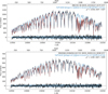 |
Fig. 6 SMART fits to IGRINS spectra for W1741–46 (top) and 2M2206–42 (bottom). The grey line is the observed IGRINS spectra, the red line is the fitted model including telluric absorption, and the blue line is the fitted model without tellurics. At the bottom of each plot is the residual between the model (including tellurics) and the observed data. The shaded blue region is the ±1σ uncertainty. |
4.4 Radial velocities
We also measured new barycentric corrected RVs using SMART for W1741–46 and 2M2206–42 and present them in Table 1. We used SMART’s barycorr function which uses astropy to calculate the barycentric corrections. RVs were corrected given the time of each observation and Earth coordinates of Gemini South (30°14.5’S, 70°44.8’W). These are the first RVs measured using high-resolution spectra from IGRINS for these objects. We provide the first RV measurement for 2M2206–42 and an updated measurement for W1741–46. We calculated the updated membership probabilities with BANYAN Σ to confirm W1741–46 as a bona fide AB Dor member with a higher membership probability of 99.9%, compared to a previous probability of 99.4% (Vos et al. 2022). We provide the first RV measurement for 2M2206–42, which increases its membership probability to 99.8% (previously 99.3%), and confirms it as a bona fide AB Dor member with its full set of kinematic information.
5 Key molecular absorptions
Mid-L dwarfs are characterised by many strong molecular absorption bands, with some atomic and molecular bands (e.g. Na, K, and H2O) strengthening as they cool to later spectral types, whereas other hydride bands such as FeH weaken with cooler spectral types as iron clouds form (Kirkpatrick 2005; Cushing et al. 2006; Yamamura et al. 2010). With JWST, we are able to observe a wide range of wavelengths near-simultaneously, allowing us to detect and characterise a broad array of molecular species for each target. This wide wavelength range also allows us to probe effects of non-equilibrium chemistry and reveal the vertical structure of the atmosphere (Cushing et al. 2006).
To identify key molecular absorption bands in the spectra, we consider cross-sections of diverse chemical species, including water (H2O), methane (CH4), carbon monoxide (CO), carbon dioxide (CO2), and ammonia (NH3). These cross-sections were calculated at a temperature of 1300 K and a pressure of 1 bar with PICASO (Batalha et al. 2020). We chose to compute our cross-sections at 1300 K, as it is the approximate midpoint Teff of our sample. The cross-sections were resampled to the same spectral resolution as our JWST spectra for ease of comparison. We show the absorption regions for these molecules in Fig. 2. In all objects, we visually identified H2O between 1.33–1.46, 1.78–1.99, 2.48–2.91, and 5.25–6.95 μm, and CO between 2.3–2.4 and 4.5–4.85 μm. However, only the three coolest dwarfs (W0047+68, 2M2244+20 and 2M0642+41) show clear signatures of CH4 between 3.2–3.45 μm and 7.3–7.9 μm, and CO2 absorption at 4.23–4.4 μm. This agrees with previous observations of the onset of CH4 absorption typically around the L7 spectral type, and strengthening towards later spectral types (Cushing et al. 2006; Suárez & Metchev 2022). 2M0642+41 has the strongest CH4 absorption in our sample, with additional absorption present in the H- and K-bands between 1.6–1.7 and 2.25–2.45 μm. At longer wavelengths for 2M0642+41, ammonia (NH3) absorption is also visible at 10.3–10.5 μm. The CH4 and NH3 absorption bands in 2M0642+41 additionally reinforces its T spectral type classification.
5.1 Water and methane
H2O and CH4 absorption dominate the spectra of mid-to-late L dwarfs, with increasing strength at later spectral types (Cushing et al. 2006). This trend was observed in a large sample of various ages, and we were interested whether our sample of young L dwarfs fit within this trend.
We measured the strength of the H2O and CH4 absorption features at 6.25 μm and 7.65 μm using the H2O and CH4 index defined in Cushing et al. (2006) and updated, for the case of CH4, in Suárez & Metchev (2022). The index is a ratio between the flux at a continuum level and the absorption feature. Thus, higher index values indicate stronger absorption features and vice versa. Using SEDA (Suárez et al. 2021b, Suárez et al., in prep.), we calculated the H2O and CH4 indices for each target and compared to targets observed with Spitzer IRS targets in Suárez & Metchev (2022, see our Fig. 7). We present our measured H2O and CH4 indices in Table 5. Our later spectral type objects tend to have higher CH4 and H2O absorption, following the general trend in Cushing et al. (2006). For both H2O and CH4, the indices for our sample lie below the median index for the Spitzer IRS sample, indicating that there is less absorption of H2O and CH4 in our young objects compared to old field objects of similar spectral types.
The shape of the water absorption features between 1–4 μm also changes with temperature. The hotter three objects (2M2206–42, 2M0355+11, and W1741–46) show more triangular and ‘peaky’ H, J, and K bands, whereas the cooler three objects (W0047+68, 2M2244+20, and 2M0642+41) have rounder features. The cooler objects have slightly lower surface gravities (see Table 4), which may suppress the shape of the H, J, and K bands relative to the water opacities (Faherty et al. 2016).
Spectral indices of H2O, CH4, and silicate.
5.2 Silicate absorption feature
The pressures and temperatures that exist in late-L dwarf atmospheres allow for the condensation of silicate grains in the visible photosphere (e.g. Lodders & Fegley 2006; Luna & Morley 2021). These condensates form silicate clouds that leave a prominent absorption feature that is detectable at 8–11 μm (Luna & Morley 2021). All objects in our sample, except 2M0642+41, show clear signatures of this silicate absorption feature (see Fig. 2). Similar to the H2O and CH4 index, the silicate index (Suárez & Metchev 2022, 2023) estimates the strength of the silicate absorption feature present by calculating the ratio between the flux at an interpolated continuum level and the flux in the absorption band. A higher silicate index corresponds to a deeper silicate feature, and indicates that clouds play a more dominant role in shaping this features. The interpolated continuum is defined by two regions on either side of the absorption region. Suárez & Metchev (2023) shifts the continuum window at longer wavelengths to redder wavelengths, compared to Suárez & Metchev (2022), to include the red wing of the silicate absorption feature, which is particularly present for young objects. However, this region at 13–14 μm has low S/N in our MIRI LRS spectra, affecting the accuracy of the interpolated continuum, and hence the calculated silicate index. The low S/N also makes it difficult to distinguish between the shape of the silicate feature at longer wavelengths. In this paper, we have used our own definition for the continuum window at longer wavelengths, which is a compromise between maintaining sensitivity to variations in the far red wing of the silicate absorption feature and sufficient S/N for the continuum. We have chosen a 0.4 μm window centred at 7.4 μm and 12.5 μm, with a linear continuum fit (see Appendix B). The 7.4 μm region lies at the end of the 6.25 μm water absorption band present in all our spectra and just before the onset of silicate absorption (Fig. 2), making it a pseudocontinuum region suitable for measuring the depth of the silicate feature. Although the 7.65 μm CH4 absorption feature overlaps this region, it appears only in spectra later than L8 (Cushing et al. 2006; Suárez & Metchev 2022), so we do not expect it to affect the silicate index measurements for our sample, except for the T1 dwarf 2M0642+41, which exhibits a strong methane feature. At this spectral type, the silicate index no longer traces the depth of silicate absorption due to the absence of that feature. However, we include silicate index values for this early T dwarf, as well as other T dwarfs in the Spitzer sample in Fig. 7 to illustrate the overall trend of the index, noting that for T dwarfs the index is more indicative of the strength of the methane feature rather than silicate absorption. We used this updated definition of the continuum with SEDA to calculate our silicate indices and present them in Table 5. We applied our updated definition to the broader Spitzer IRS sample from Suárez & Metchev (2022) to ensure consistency.
There is no 8–11 μm silicate absorption feature visible in the spectrum of 2M0642+41. These silicate clouds have sunk deep beyond the mid-IR photosphere, which is typical of T dwarfs (Ackerman & Marley 2001; Saumon & Marley 2008; Cushing et al. 2006; Suárez et al. 2021a), reinforcing our updated spectral classification. Absorption from other molecules (e.g. CH4) in 2M0642+41 change the continuum in such a way that the divided spectrum does not show the silicate features but rather the appearance of methane. The presence of methane affects the short-wavelength continuum region by reducing the flux, so the interpolated continuum is below the observed flux in the silicate absorption region. The abundance of methane increases as Teff decreases towards later T dwarfs, so this has less of an effect on continuum interpolation for our objects, which are earlier L-type dwarfs. However, we still expect there to be silicate clouds present in the NIR photosphere of 2M0642+41 which can be indirectly observed at shorter wavelengths and can be better revealed with future retrievals. Previous atmospheric retrievals of T dwarfs have found evidence of deeper silicates (Vos et al. 2023; Nasedkin et al. 2025). 2M0642+41 is the most variable at 3.6 μm in our sample, so this non-detection of the mid-IR silicate absorption feature contradicts expectations that these silicate clouds drive variability. However, different cloud compositions, such as iron, could have a greater effect on variability at NIR wavelengths.
We compare the silicate indices of our targets to the Spitzer IRS sample from Suárez & Metchev (2022) in Fig. 7. The Spitzer IRS sample of brown dwarfs consists of more old field dwarfs that are silicate rich than young silicate-rich objects. All our targets have a measured silicate index greater than the median of the Spitzer IRS sample, particular W1741–46, which has the highest silicate index yet measured. Conversely, as mentioned in Sect. 5.1, all objects have a H2O lower than the median, suggesting an anticorrelation between silicate and H2O absorptions. Lower gravity objects show evidence of thicker silicate clouds (Marley et al. 2012; Faherty et al. 2016; Liu et al. 2016; Vos et al. 2022), which could block observations of water in the atmosphere (Suárez & Metchev 2023; Suárez et al., in prep.). Our sample consists of only young brown dwarfs, so our low H2O indices and high silicate indices may be indicative of their youth. This can be supported by the fact that young, low gravity L dwarfs tend to have redder NIR colours and are more variable (Kirkpatrick et al. 2008; Faherty et al. 2016; Suárez & Metchev 2022), suggesting that clouds are more prominent in young L dwarf atmospheres.
We isolated the shape of the silicate feature by dividing the flux by the interpolated continuum, as described above. Suárez & Metchev (2023) observed a difference in the shape of the silicate feature between young and old brown dwarfs, where their young sample had a broader and more asymmetric absorption feature that was more redshifted compared to their old sample. This is thought to be caused by larger, heavier iron-rich silicate grains which sediment less efficiently in young objects (Luna & Morley 2021; Suárez & Metchev 2023). Similarly, we investigate the diversity in the shape of the silicate feature in our sample through comparisons with the mean silicate feature of our spectra. We present this comparison in Fig. 8. Following a similar procedure as in Suárez & Metchev (2023), we scaled the silicate feature to the mean flux in a 0.6 μm window centred at 9.3 μm. This scaling removes differences in the silicate column density, and instead highlights the diversity between the shapes, which is affected by the composition of the silicate clouds (e.g. Luna & Morley 2021; Suárez & Metchev 2023; Hoch et al. 2025; Mollière et al. 2025). We also calculated the wavelength at peak absorption by fitting a third-order polynomial to the silicate feature between 8.5–11 μm and estimating the wavelength at the minimum.
From Fig. 8, we can clearly see there is a great diversity just within our sample of L type AB Dor objects. The silicate feature of W0047+68 and 2M2244+20 are almost identical to each other, sharing similar widths and peak absorption wavelengths. These peak absorption wavelengths are relatively shifted towards longer wavelengths compared to the rest of the sample. These objects also have similarities in the absorption of other molecules, including H2O and CH4, as indicated by the measured molecular indices in Fig. 7 and their full spectra in Fig. 2. This suggests dependencies between cloud condensation and molecular abundances, including C/O ratios (Luna & Morley 2021). On the other hand, the silicate features of 2M0355+11 and W1741–46 are shifted to bluer wavelengths and broader compared to the other objects. W1741–46 has similar spectral type and colour to W0047+68 and 2M2244+20, but its silicate feature is shifted to bluer wavelengths.
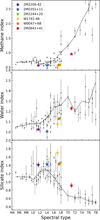 |
Fig. 7 Calculated CH4 (top), H2O (middle), and silicate (bottom) indices for our sample (coloured stars) compared to those from the Spitzer IRS sample (shown as black points). The spectral types of W0047+68 and 2M2244+20 have an additional −0.15 and +0.15, respectively, for visualisation purposes. The dashed black line represents the median index for the bins of two spectral types in the Spitzer IRS sample using our updated silicate index definition in the bottom panel. |
5.3 Trends with inclination
Suárez et al. (2023) suggested that brown dwarfs viewed equator-on exhibited more opaque silicate clouds, while those viewed pole-on have fewer clouds. This also correlates with the colour anomaly, with redder objects having a more equator-on inclination angle and greater silicate index (Vos et al. 2017). In Fig. 9, we define our colour anomaly as the difference between the J-KS MKO colour and the mean J-KS MKO colour of all the young brown dwarfs obtained from the UltracoolSheet (Best et al. 2024). Our sample provides a unique opportunity to test the correlation between cloudiness and inclination angle, as our brown dwarfs are the same age, unlike the broader Spitzer sample analysed in Suárez et al. (2023). This eliminates any possibilities of cloud variations due to surface gravity, which is similar for all objects (log g ~ 4.4–4.8). Figure 9 shows the trend between the silicate index and inclination angle and compares it to the sample previously analysed in Suárez et al. (2023). We did not include 2M0642+41 in our analysis because its silicate index is more indicative of the depth of the methane feature than of silicate absorption. Most of our objects (W0047+68, 2M2206–42, 2M2244+20, and tentatively 2M0355+11) follow the previously observed trend of a strong positive correlation between inclination and silicate index. This trend suggests that lower latitude clouds have redder colours and deeper silicate features.
It is clear, however, that W1741–46 is an outlier in our sample with an unusually high silicate index of 1.7 ± 0.1 and low inclination angle of ![Mathematical equation: $\[i=23.6_{-3.6}^{+3.4^{\circ}}\]$](/articles/aa/full_html/2026/05/aa58421-25/aa58421-25-eq22.png) (viewed near pole-on). According to the correlation between inclination and silicate index, and given its nearly pole-on orientation, W1741–46 should exhibit very weak silicate absorption. However, its MIRI spectrum reveals a strong silicate feature. Tan & Showman (2021) suggest that latitudinal cloud distribution is determined by the object’s rotation rate. For faster rotating objects (P ≤ 2 h), we expect the cloudy equatorial bands to be more prominent compared to the clearer poles due to Coriolis effects at higher altitudes near the equator. Since W1741–46 has a rotational period of P ~ 15 h, the difference between the cloud distribution at the equator and the pole is not as significant, suggesting that the whole atmosphere could be cloudy. We plan on investigating this object with atmospheric retrievals in future work to determine the cause of the unusually deep silicate feature.
(viewed near pole-on). According to the correlation between inclination and silicate index, and given its nearly pole-on orientation, W1741–46 should exhibit very weak silicate absorption. However, its MIRI spectrum reveals a strong silicate feature. Tan & Showman (2021) suggest that latitudinal cloud distribution is determined by the object’s rotation rate. For faster rotating objects (P ≤ 2 h), we expect the cloudy equatorial bands to be more prominent compared to the clearer poles due to Coriolis effects at higher altitudes near the equator. Since W1741–46 has a rotational period of P ~ 15 h, the difference between the cloud distribution at the equator and the pole is not as significant, suggesting that the whole atmosphere could be cloudy. We plan on investigating this object with atmospheric retrievals in future work to determine the cause of the unusually deep silicate feature.
We notice a tentative trend with inclination when observing the shape of the silicate feature in Fig. 8. The wavelength at peak absorption appears to get progressively shifted towards bluer wavelengths as the viewing angle transitions from equator-on to pole-on. The onset of the silicate absorption is also shifted towards redder wavelengths for equator-on targets. The most significant differences in the shape of the silicate feature appear to be at shorter wavelengths, although the noise at longer wavelengths in the MIRI LRS spectra make it difficult to accurately discern between each spectrum. Luna & Morley (2021) predicts that different grain size distributions of the same composition can produce silicate features that peak at slightly different wavelengths. More small grains will cause the absorption to be strongest at shorter wavelengths and vice versa. Our observed trend suggests that there will be more larger sized grains at the equator. In addition, they predict that grains of different compositions – for example, enstatite and forsterite – produce similar silicate features with only slight shifts in wavelength. Future work with atmospheric retrievals will constrain these cloud properties (e.g. Burningham et al. 2021; Vos et al. 2023; Mollière et al. 2025) so we can further understand how these clouds vary from equator to pole.
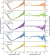 |
Fig. 8 Isolated silicate absorption features of the objects in our AB Dor sample, after continuum removal. The spectra of the silicate feature has been ordered with inclination angle, with objects viewed more equator-on towards the top and objects viewed more pole-on towards the bottom. Left panels: direct comparison of the shape of the silicate feature with the mean silicate feature of our sample (dotted black line), with the shaded region representing one standard deviation. The vertical dashed line in the left panels shows the wavelength at peak absorption for each object. Right panels: deviation from the mean silicate feature for each object. |
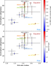 |
Fig. 9 Correlation between the inclination and the silicate index for our sample (stars) compared with the Spitzer sample (circles) from Suárez et al. (2023). VHS 1256 b is also included with a triangle marker and black error bars. The upper panel is colour-coded according to the J-KS MKO colour anomaly calculated from young objects in the Ultracool-Sheet (Best et al. 2024). The lower panel is colour-coded according to the spectral type of each object. 2M0642+41 is not present in this figure, as it is a T dwarf with no silicate absorption feature present in the spectrum. |
6 Spectral comparisons
6.1 Long-term variability
Long-term variability spanning multiple rotational periods, months or even years, has previously been detected on L/T transition dwarfs, for example VHS 1256 b and WISE J104915.57531906.1AB (hereafter WISE 1049AB; Luhman 2013; Apai et al. 2017; Zhou et al. 2022; Fuda et al. 2024). Zhou et al. (2022) detected long-term variability in VHS 1256 b over 1–2 years in the NIR wavelength range. VHS 1256 b is spectrally similar to our sample, and so we expect there to be similar long-term variability trends in our spectra. Chen et al. (2025) detected longterm variability across 1–12 μm, including in the silicate feature, for WISE 1049 AB, indicating that similar long-term variability in the silicate feature for the objects in our sample may occur.
Suárez & Metchev (2022) previously analysed archival mid-IR spectra (5–14 μm) for 2M0355+11 and 2M2244+20 with Spitzer IRS, providing a unique opportunity to search for longterm variability. 2M0355+11 was observed on 2008-10-10 and 2M2244+20 was observed on 2004-12-10. We plot these Spitzer spectra alongside our MIRI spectra in Fig. 10 to determine whether there is evidence of variability between epochs.
For 2M0355+11 there is a flux difference of up to 10% between the spectra at mid-MIRI wavelengths (~7–10 μm). However, since the spectra were observed with different instruments, there may be systematic differences that are not yet known. Because of this, we cannot be certain that the difference we observe is due to the intrinsic variability of the object or due to systematic uncertainties between Spitzer/IRS and JWST/MIRI. Multiple epochs from JWST MIRI will allow us to determine the mid-IR variability properties of 2M0355+11.
For 2M2244+20 we have good agreement between the observed spectra across the two epochs. However, the Spitzer IRS spectrum is significantly noisier. Since the spectra from both epochs are similar, we cannot identify any long-term variability in the silicate feature. Additional MIRI LRS observations, however, can more precisely measure the variability in this wavelength range without the added complication of systematics between different instruments.
The silicate index is also a measurement of variability, as silicate-rich L-dwarfs tend to be variable (Suárez & Metchev 2022). This measure is less sensitive to systematics as it is a relative measurement dependent on the same spectrum. Using the Spitzer IRS spectrum, we measured the silicate index for 2M0355+11 to be 1.43 ± 0.03 and for 2M2244+20 to be 1.52 ± 0.2. These silicate indices agree with our measurements using JWST MIRI spectra,so we cannot confirm long-term variability in our objects. However, our high silicate indices suggest that long-term variability may exist in 2M0355+11 and 2M2244+20, and we would require more time series observations to confirm.
6.2 Comparison with directly imaged exoplanets
Objects in our sample have similar colours and magnitudes to other previously known planetary mass objects (e.g. VHS 1256 b, PSO J318, and YSES 1 c; see Fig. 1). We compare their spectra to examine whether there are other similarities. These objects are also similar to directly imaged exoplanets, such as HR 8799 bcd, so these comparisons will allow us to determine if our sample are good exoplanet analogues.
VHS 1256 b (Gauza et al. 2015) is a young (140 ± 20 Myr; Dupuy et al. 2023) planetary mass companion that lies on the mass boundary between planets and brown dwarfs with an age very similar to our AB Dor objects (~133 Myr). VHS 1256 b was the first planetary-mass object to be observed by JWST to produce a 1–20 μm spectrum (Miles et al. 2023). There have been many studies on the variability and atmosphere of the most variable planetary mass object known, VHS 1256 b (e.g. Rich et al. 2016; Bowler et al. 2020; Zhou et al. 2022), revealing complex cloudy atmospheres causing highly variable time-series observations.
VHS 1256 b lies along the L–T transition with spectral type L7 ± 1.5 and ![Mathematical equation: $\[\log ~\left(\frac{L_{\mathrm{bol}}}{L_{\odot}}\right)=-4.60 \pm 0.05\]$](/articles/aa/full_html/2026/05/aa58421-25/aa58421-25-eq23.png) (Miles et al. 2023), very similar to our sample (see Fig. 1, Table 4). Thus, this object provides an excellent scientific comparison for our sample. VHS 1256 b also shares photometric and spectroscopic similarities with other directly imaged exoplanets such as HR 8799 bcde (Marois et al. 2008, 2010), allowing us to view our sample as exoplanet analogues.
(Miles et al. 2023), very similar to our sample (see Fig. 1, Table 4). Thus, this object provides an excellent scientific comparison for our sample. VHS 1256 b also shares photometric and spectroscopic similarities with other directly imaged exoplanets such as HR 8799 bcde (Marois et al. 2008, 2010), allowing us to view our sample as exoplanet analogues.
W0047+68 was previously reported to be similar to VHS 1256 b (e.g. Zhou et al. 2022). In our analysis, we compared the spectra of all our objects with VHS 1256 b’s spectrum and plot VHS 1256 b alongside W0047+68 and 2M2244+20 in Fig. 11. We found that 2M2244+20 has the most similar spectrum to VHS 1256 b (Miles et al. 2023), in both the shape of the absorption features and the amount of flux emitted. This is the first time that the entire SEDs have been compared, allowing us to draw novel conclusions. We down-sampled the VHS 1256 b spectrum using SpectRes (Carnall 2017) to match the spectral resolution achieved by NIRSpec Prism and MIRI LRS. W0047+68 also has a similar spectrum, but is slightly more luminous than VHS 1256 b (see Table 4 and Fig. 11). This observed similarity is supported by their nearby positions on the colour-magnitude diagram in Fig. 1. It is notable that W0047+68 and 2M2244+20 also have mass and effective temperatures consistent within the uncertainties with VHS 1256 b (M = 19 ± 5 MJup, Teff = 1240 ± 50 K; Dupuy et al. 2020).
We have also analysed the silicate feature of VHS 1256 b. We calculated the silicate absorption features from a MIRI MRS spectrum (Miles et al. 2023) that was downsampled to match our MIRI LRS resolution. Both the silicate index and the shape of the silicate feature resemble that of W0047+68 and 2M2244+20 (see Fig. 11). VHS 1256 b is also viewed equator-on (Zhou et al. 2020) and supports the trend between inclination and silicate index (Fig. 9).
VHS 1256 b fits well within our sample with very similar spectra, which emphasises how the fundamental parameters of brown dwarfs, including age, temperature and mass shape their spectra. The HR8799 directly imaged exoplanet system also lies in a similar position on the colour-magnitude diagram, indicating that our sample of young AB Dor objects can be used as excellent exoplanet analogues. In order to better understand the complex atmospheric chemistry and dynamics of similar hot gas giants, we can study W0047+68 and 2M2244+20, which we can observe much more easily than directly imaged exoplanets.
We also compared our objects to spectra from the directly imaged isolated planetary mass object PSO J318 (Mollière et al. 2025) and the imaged companion YSES-1 c (Hoch et al. 2025) in Fig. 11, focusing on the silicate absorption feature observed by MIRI. PSO J318 also has a similar spectrum to W0047+68 and 2M2244+20, emphasising our sample as analogues to planetary mass objects. Hoch et al. (2025) identified that YSES-1 c has an unusual silicate feature with a redder onset, which is made clear in the comparison in Fig. 11. YSES-1 c is an exoplanet viewed equator on (i ~ 90°; Roberts et al. 2025). The onset of its silicate feature shifted towards redder wavelengths supports our tentative trend between inclination and silicate absorption peak discussed in Sect. 5.3, and suggests that this trend may also be applied to exoplanets.
W0047+68 and 2M2244+20 have similar magnitudes, colours, spectral types and ages to the HR 8799 planets (see Fig. 1), which have dynamical masses between 6–10 MJup (Brandt et al. 2021; Zurlo et al. 2022). This indicates that these objects may have planetary masses. Dynamical masses are not possible for our isolated objects, but the evolutionary models predict a bimodal mass distribution (see Appendix A), suggesting that these objects may also have planetary masses. Future studies comparing dynamical with evolutionary model masses for companions are crucial for assessing the accuracy of evolutionary models.
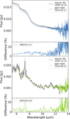 |
Fig. 10 Spectral comparison between Spitzer IRS observations (Suárez & Metchev 2022) and our JWST MIRI LRS observations for 2M0355+11 and 2M2244+20. The Spitzer spectra are shown in black and our spectra are coloured. Top two panels: Comparison for 2M0355+11. Bottom two panels: Comparison for 2M2244+20. The uncertainties are shown as the shaded envelope region. Below each spectral comparison is the relative flux difference (max/min − 1). |
7 Conclusions
We have presented the first full 0.6–14 μm, R ~ 100 JWST NIRSpec and MIRI spectra for a sample of five young, coeval objects in the AB Dor moving group and one young object in the Oceanus moving group. We conducted a full SED analysis to measure the fundamental parameters of each object in order to fully characterise our sample. We also analysed molecular absorption bands, in particular the silicate feature present at 8–11 μm, and investigated the possibility of latitudinal atmospheric dependencies. From this analysis, we have derived the following conclusions:
All objects within our sample are diverse. Our sample of AB Dor objects span from early to late L dwarfs, and we found that our objects span a range of Teff ~ 1000–1700 K, log g ~ 4.1–4.8, a radius of ~1.20–1.28 RJup, and M ~ 8–34 MJup (Table 4). We found that 2M2206–42 and 2M0355+11 are similar to each other, and 2M2244+20 and W0047+68 are similar. These pairs have similar spectral types to each other, so it is expected that they also have similar spectra. These two pairs could be studied together in future work in order to examine their similarities as well as the differences with respect to the full sample;
Although 2M0642+41 has the highest variability amplitude in our sample, it has no distinguishable silicate absorption feature at 10 μm. This is because at 2M0642+41’s temperature of ~1070 K and spectral type T1, the silicate clouds have most likely sunk below the photosphere. However, silicate clouds can still exist in its deeper NIR photosphere and impact its NIRSpec spectrum. Future atmospheric retrievals will be able to reveal the atmospheric structure in greater detail and determine the cause of 2M0642+41 ‘s high amplitude variability;
W1741–46 is a counterexample to the suggested trend between silicate index and inclination. This object has an unusually high silicate index (1.7 ± 0.1) for its close to pole-on orientation (
![Mathematical equation: $\[i=23.6_{-3.6}^{+3.4^{\circ}}\]$](/articles/aa/full_html/2026/05/aa58421-25/aa58421-25-eq24.png) ). This does not follow the expected correlation between silicate index and inclination identified in Suárez et al. (2023). The silicate indices of the other objects in our sample agree with the trend observed in Suárez et al. (2023). However, they have very similar silicate indices, which may be due to our selection of a uniform sample. The silicate index of W1741–46 is also one of the highest measured in a broader sample of brown dwarfs, indicating that W1741–46 has the most prominent silicate absorption analysed so far. More late L dwarfs with low inclination angles are required to confirm whether W1741–46 is an outlier or if an opposite trend is observed in later L dwarfs. This motivates future observations of late L dwarfs with low inclination angles. In future work, we will investigate the cause of this unusual silicate absorption feature by running atmospheric retrievals with Brewster (Burningham et al. 2017);
). This does not follow the expected correlation between silicate index and inclination identified in Suárez et al. (2023). The silicate indices of the other objects in our sample agree with the trend observed in Suárez et al. (2023). However, they have very similar silicate indices, which may be due to our selection of a uniform sample. The silicate index of W1741–46 is also one of the highest measured in a broader sample of brown dwarfs, indicating that W1741–46 has the most prominent silicate absorption analysed so far. More late L dwarfs with low inclination angles are required to confirm whether W1741–46 is an outlier or if an opposite trend is observed in later L dwarfs. This motivates future observations of late L dwarfs with low inclination angles. In future work, we will investigate the cause of this unusual silicate absorption feature by running atmospheric retrievals with Brewster (Burningham et al. 2017);We tentatively find that the shape of the silicate feature depends on inclination. Objects viewed equator-on tend to have a silicate feature shifted towards redder wavelengths, whereas those viewed closer to pole-on tend to have a silicate feature shifted towards bluer wavelengths (Fig. 8). The shape of the silicate feature could provide insights into the chemical composition and/or grain sizes of the silicate clouds, which require detailed modelling to further analyse this trend. In future work, we plan to further investigate whether grain size or composition is responsible for the observed silicate absorption differences. This will allow us to determine the cloud structure and composition of each object and how it varies from equator-to-pole. Further analysis is also required to rule out any other factors that could be contributing to this trend (e.g. Teff). Observations of other young objects with known inclinations (e.g. VHS 1256 b, 2MASS J05012406-0010452 (Reid et al. 2008), 2MASS J14252798-3650229 (Kendall et al. 2004), YSES–1 c (Bohn et al. 2020), PSO J318) will also help determine whether their silicate features fit within potential trends in our young sample;
No significant long-term variability was detected in the silicate feature of the two objects with literature mid-IR spectra (Fig. 10). We had expected to see a variation in the silicate feature corresponding to previously detected variability, but this was not observed in our comparisons. However, this is only based on comparisons of two snapshots of spectra, and variations may still be detectable if more spectra are obtained over time. The spectra were also obtained from different instruments, so systematics may have prevented us from probing this long-term variability;
The objects W0047+68 and 2M2244+20 are excellent exoplanet analogues and have similarities to VHS 1256 b, another planetary mass object that has similarities with known exoplanets. The two objects also have spectra similar to the planetary mass object PSO J318. The similarities between the spectra reinforce our motivation to study this sample of young brown dwarfs to further understand directly imaged exoplanets, such as the HR8799 system.
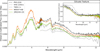 |
Fig. 11 Comparison between our objects W0047+68 and 2M2244+20 (coloured lines) and other directly imaged exoplanets: PSO J318, VHS 1256 b, and YSES-1 c (dashed, solid, and dotted black lines, respectively). For ease of comparison, the spectra of each object not included in our sample were re-normalised to match the spectral resolutions of our JWST NIRSpec Prism and MIRI LRS spectra. To highlight the 8–11 μm silicate absorption feature, each spectrum was normalised to the flux in a 0.2 μm window centred at 6.2 μm and shown in the inset. Objects in our sample are most similar to VHS 1256 b. |
Acknowledgements
We would like to thank the anonymous referee for their detailed comments and suggestions that have improved the paper. ML and JMV acknowledge support from a Royal Society – Research Ireland University Research Fellowship (URF/1/221932, RF/ERE/221108). ML acknowledges support from Trinity College Dublin via a Trinity Research Doctoral Award. BB acknowledges support from UK Research and Innovation Science and Technology Facilities Council [ST/X001091/1]. This work is based [in part] on observations made with the NASA/ESA/CSA James Webb Space Telescope. The data were obtained from the Mikulski Archive for Space Telescopes at the Space Telescope Science Institute, which is operated by the Association of Universities for Research in Astronomy, Inc., under NASA contract NAS 5-03127 for JWST. These observations are associated with program #3486. Some/all of the data presented in this paper were obtained from the Mikulski Archive for Space Telescopes (MAST) at the Space Telescope Science Institute. The specific observations analyzed can be accessed via https://doi.org/10.17909/ws6v-js74. STScI is operated by the Association of Universities for Research in Astronomy, Inc., under NASA contract NAS5–26555. Support to MAST for these data is provided by the NASA Office of Space Science via grant NAG5–7584 and by other grants and contracts. This work has benefitted from The UltracoolSheet at http://bit.ly/UltracoolSheet, maintained by Will Best, Trent Dupuy, Michael Liu, Aniket Sanghi, Rob Siverd, and Zhoujian Zhang, and developed from compilations by Dupuy & Liu (2012, ApJS, 201, 19), Dupuy & Kraus (2013, Science, 341, 1492), Deacon et al. (2014, ApJ, 792, 119), Liu et al. (2016, ApJ, 833, 96), Best et al. (2018, ApJS, 234, 1), Best et al. (2021, AJ, 161, 42), Sanghi et al. (2023, ApJ, 959, 63), and Schneider et al. (2023, AJ, 166, 103). This work used The Immersion Grating Infrared Spectrometer (IGRINS) was developed under a collaboration between the University of Texas at Austin and the Korea Astronomy and Space Science Institute (KASI) with the financial support of the US National Science Foundation under grants AST-1229522, AST-1702267 and AST-1908892, McDonald Observatory of the University of Texas at Austin, the Korean GMT Project of KASI, the Mt. Cuba Astronomical Foundation and Gemini Observatory. The RRISA is maintained by the IGRINS Team with support from McDonald Observatory of the University of Texas at Austin and the US National Science Foundation under grant AST-1908892. This research made use of the Montreal Open Clusters and Associations (MOCA) database, operated at the Montréal Planétarium (Gagné et al. 2026).
References
- Ackerman, A. S., & Marley, M. S. 2001, ApJ, 556, 872 [Google Scholar]
- Allard, F., Homeier, D., & Freytag, B. 2012, Philos. Trans. Roy. Soc. Lond. A, 370, 2765 [NASA ADS] [Google Scholar]
- Allers, K. N., & Liu, M. C. 2013, ApJ, 772, 79 [NASA ADS] [CrossRef] [Google Scholar]
- Allers, K. N., Gallimore, J. F., Liu, M. C., & Dupuy, T. J. 2016, ApJ, 819, 133 [Google Scholar]
- Apai, D., Radigan, J., Buenzli, E., et al. 2013, ApJ, 768, 121 [NASA ADS] [CrossRef] [Google Scholar]
- Apai, D., Karalidi, T., Marley, M. S., et al. 2017, Science, 357, 683 [Google Scholar]
- Artigau, É., Bouchard, S., Doyon, R., & Lafrenière, D. 2009, ApJ, 701, 1534 [NASA ADS] [CrossRef] [Google Scholar]
- Baraffe, I., Homeier, D., Allard, F., & Chabrier, G. 2015, A&A, 577, A42 [NASA ADS] [CrossRef] [EDP Sciences] [Google Scholar]
- Bardalez Gagliuffi, D. C., Faherty, J. K., Li, Y., et al. 2021, ApJ, 922, L43 [NASA ADS] [CrossRef] [Google Scholar]
- Bardalez Gagliuffi, D. C., Balmer, W. O., Pueyo, L., et al. 2025, ApJ, 988, L18 [Google Scholar]
- Batalha, N., Freedman, R., Gharib-Nezhad, E., & Lupu, R. 2020, Resampled Opacity Database for PICASO [Google Scholar]
- Best, W. M. J., Liu, M. C., Magnier, E. A., et al. 2015, ApJ, 814, 118 [CrossRef] [Google Scholar]
- Best, W. M. J., Liu, M. C., Magnier, E. A., & Dupuy, T. J. 2021, AJ, 161, 42 [Google Scholar]
- Best, W. M. J., Dupuy, T. J., Liu, M. C., et al. 2024, The UltracoolSheet: Photometry, Astrometry, Spectroscopy, and Multiplicity for 4000+ Ultracool Dwarfs and Imaged Exoplanets [Google Scholar]
- Best, W. M. J., Sanghi, A., Liu, M. C., Magnier, E. A., & Dupuy, T. J. 2024, ApJ, 967, 115 [NASA ADS] [CrossRef] [Google Scholar]
- Biller, B. A., Vos, J. M., Zhou, Y., et al. 2024, MNRAS, 532, 2207 [NASA ADS] [CrossRef] [Google Scholar]
- Blake, C. H., Charbonneau, D., & White, R. J. 2010, ApJ, 723, 684 [Google Scholar]
- Bohn, A. J., Kenworthy, M. A., Ginski, C., et al. 2020, ApJ, 898, L16 [Google Scholar]
- Bowler, B. P., Zhou, Y., Morley, C. V., et al. 2020, ApJ, 893, L30 [NASA ADS] [CrossRef] [Google Scholar]
- Brandt, G. M., Brandt, T. D., Dupuy, T. J., Michalik, D., & Marleau, G.-D. 2021, ApJ, 915, L16 [NASA ADS] [CrossRef] [Google Scholar]
- Burgasser, A. J., Kirkpatrick, J. D., Brown, M. E., et al. 2002, ApJ, 564, 421 [NASA ADS] [CrossRef] [Google Scholar]
- Burningham, B., Marley, M. S., Line, M. R., et al. 2017, MNRAS, 470, 1177 [NASA ADS] [CrossRef] [Google Scholar]
- Burningham, B., Faherty, J. K., Gonzales, E. C., et al. 2021, MNRAS, 506, 1944 [NASA ADS] [CrossRef] [Google Scholar]
- Burrows, A., Hubbard, W. B., Lunine, J. I., & Liebert, J. 2001, Rev. Mod. Phys., 73, 719 [Google Scholar]
- Burrows, A., Sudarsky, D., & Hubeny, I. 2006, ApJ, 640, 1063 [Google Scholar]
- Bushouse, H., Eisenhamer, J., Dencheva, N., et al. 2024, JWST Calibration Pipeline [Google Scholar]
- Cardelli, J. A., Clayton, G. C., & Mathis, J. S. 1989, ApJ, 345, 245 [Google Scholar]
- Carnall, A. C. 2017, arXiv e-prints [arXiv:1705.05165] [Google Scholar]
- Chabrier, G., Baraffe, I., Phillips, M., & Debras, F. 2023, A&A, 671, A119 [NASA ADS] [CrossRef] [EDP Sciences] [Google Scholar]
- Chen, X., Biller, B. A., Tan, X., et al. 2025, MNRAS, 539, 3758 [Google Scholar]
- Cruz, K. L., Kirkpatrick, J. D., & Burgasser, A. J. 2009, AJ, 137, 3345 [NASA ADS] [CrossRef] [Google Scholar]
- Cruz, K. L., Núñez, A., Burgasser, A. J., et al. 2018, AJ, 155, 34 [NASA ADS] [CrossRef] [Google Scholar]
- Cushing, M. C., Roellig, T. L., Marley, M. S., et al. 2006, ApJ, 648, 614 [Google Scholar]
- Dahn, C. C., Harris, H. C., Vrba, F. J., et al. 2002, AJ, 124, 1170 [NASA ADS] [CrossRef] [Google Scholar]
- Dupuy, T. J., Liu, M. C., Magnier, E. A., et al. 2020, RNAAS, 4, 54 [Google Scholar]
- Dupuy, T. J., Liu, M. C., Evans, E. L., et al. 2023, MNRAS, 519, 1688 [Google Scholar]
- Faherty, J. K., Rice, E. L., Cruz, K. L., Mamajek, E. E., & Núñez, A. 2013, AJ, 145, 2 [CrossRef] [Google Scholar]
- Faherty, J. K., Riedel, A. R., Cruz, K. L., et al. 2016, ApJS, 225, 10 [Google Scholar]
- Filippazzo, J. C., Rice, E. L., Faherty, J., et al. 2015, ApJ, 810, 158 [Google Scholar]
- Fuda, N., & Apai, D. 2024, ApJ, 975, L32 [Google Scholar]
- Fuda, N., Apai, D., Nardiello, D., et al. 2024, ApJ, 965, 182 [Google Scholar]
- Gagné, J., Faherty, J. K., Cruz, K. L., et al. 2015, ApJS, 219, 33 [CrossRef] [Google Scholar]
- Gagné, J., Fontaine, G., Simon, A., & Faherty, J. K. 2018a, ApJ, 861, L13 [Google Scholar]
- Gagné, J., Mamajek, E. E., Malo, L., et al. 2018b, ApJ, 856, 23 [Google Scholar]
- Gagné, J., Moranta, L., Faherty, J. K., et al. 2023, ApJ, 945, 119 [CrossRef] [Google Scholar]
- Gagné, J., Moranta, L., Faherty, J. K., et al. 2026, arXiv e-prints [arXiv:2602.15695] [Google Scholar]
- Gaia Collaboration (Vallenari, A., et al.) 2023, A&A, 674, A1 [NASA ADS] [CrossRef] [EDP Sciences] [Google Scholar]
- Gao, P., Wakeford, H. R., Moran, S. E., & Parmentier, V. 2021, J. Geophys. Res. (Planets), 126, e06655 [NASA ADS] [Google Scholar]
- Gauza, B., Béjar, V. J. S., Pérez-Garrido, A., et al. 2015, ApJ, 804, 96 [NASA ADS] [CrossRef] [Google Scholar]
- Ge, H., Zhang, X., Fletcher, L. N., et al. 2019, AJ, 157, 89 [NASA ADS] [CrossRef] [Google Scholar]
- Gizis, J. E., Faherty, J. K., Liu, M. C., et al. 2012, AJ, 144, 94 [NASA ADS] [CrossRef] [Google Scholar]
- Gizis, J. E., Allers, K. N., Liu, M. C., et al. 2015, ApJ, 799, 203 [NASA ADS] [CrossRef] [Google Scholar]
- Grant, D., Lewis, N. K., Wakeford, H. R., et al. 2023, ApJ, 956, L32 [NASA ADS] [CrossRef] [Google Scholar]
- Hoch, K. K. W., Rowland, M., Petrus, S., et al. 2025, Nature, 643, 938 [Google Scholar]
- Hsu, C.-C., Burgasser, A. J., Theissen, C. A., et al. 2021, ApJS, 257, 45 [NASA ADS] [CrossRef] [Google Scholar]
- Hurt, S. A., Liu, M. C., Zhang, Z., et al. 2024, ApJ, 961, 121 [NASA ADS] [CrossRef] [Google Scholar]
- Jakobsen, P., Ferruit, P., Alves de Oliveira, C., et al. 2022, A&A, 661, A80 [NASA ADS] [CrossRef] [EDP Sciences] [Google Scholar]
- Kaplan, K., Lee, J.-J., Sawczynec, E., & Kim, H.-J. 2024, igrins/plp [Google Scholar]
- Kendall, T. R., Delfosse, X., Martín, E. L., & Forveille, T. 2004, A&A, 416, L17 [NASA ADS] [CrossRef] [EDP Sciences] [Google Scholar]
- Kirkpatrick, J. D. 2005, ARA&A, 43, 195 [Google Scholar]
- Kirkpatrick, J. D., Reid, I. N., Liebert, J., et al. 2000, AJ, 120, 447 [NASA ADS] [CrossRef] [Google Scholar]
- Kirkpatrick, J. D., Cruz, K. L., Barman, T. S., et al. 2008, ApJ, 689, 1295 [NASA ADS] [CrossRef] [Google Scholar]
- Kirkpatrick, J. D., Gelino, C. R., Faherty, J. K., et al. 2021, ApJS, 253, 7 [Google Scholar]
- Knapp, G. R., Leggett, S. K., Fan, X., et al. 2004, AJ, 127, 3553 [Google Scholar]
- Kumar, S. S. 1963, ApJ, 137, 1121 [Google Scholar]
- Lang, D., Hogg, D. W., & Schlegel, D. J. 2016, AJ, 151, 36 [Google Scholar]
- Lawrence, A., Warren, S. J., Almaini, O., et al. 2007, MNRAS, 379, 1599 [Google Scholar]
- Lew, B. W. P., Apai, D., Zhou, Y., et al. 2016, ApJ, 829, L32 [NASA ADS] [CrossRef] [Google Scholar]
- Liu, M. C., Magnier, E. A., Deacon, N. R., et al. 2013, ApJ, 777, L20 [NASA ADS] [CrossRef] [Google Scholar]
- Liu, M. C., Dupuy, T. J., & Allers, K. N. 2016, ApJ, 833, 96 [NASA ADS] [CrossRef] [Google Scholar]
- Lodders, K., & Fegley, B. 2002, Icarus, 155, 393 [Google Scholar]
- Lodders, K., & Fegley, Jr., B. 2006, in Astrophysics Update 2, ed. J. W. Mason, 1 [Google Scholar]
- Luhman, K. L. 2013, ApJ, 767, L1 [NASA ADS] [CrossRef] [Google Scholar]
- Luhman, K. L. 2014, ApJ, 786, L18 [Google Scholar]
- Luna, J. L., & Morley, C. V. 2021, ApJ, 920, 146 [NASA ADS] [CrossRef] [Google Scholar]
- Mace, G. N., Kirkpatrick, J. D., Cushing, M. C., et al. 2013, ApJS, 205, 6 [Google Scholar]
- Mace, G., Kim, H., Jaffe, D. T., et al. 2016, SPIE Conf. Ser., 9908, 99080C [NASA ADS] [Google Scholar]
- Mace, G., Sokal, K., Lee, J.-J., et al. 2018, SPIE Conf. Ser., 10702, 107020Q [NASA ADS] [Google Scholar]
- Mader, E., Zhang, Z., Fortney, J. J., et al. 2026, AJ, 171, 198 [Google Scholar]
- Marley, M. S., Seager, S., Saumon, D., et al. 2002, ApJ, 568, 335 [NASA ADS] [CrossRef] [Google Scholar]
- Marley, M. S., Saumon, D., & Goldblatt, C. 2010, ApJ, 723, L117 [NASA ADS] [CrossRef] [Google Scholar]
- Marley, M. S., Saumon, D., Cushing, M., et al. 2012, ApJ, 754, 135 [Google Scholar]
- Marois, C., Macintosh, B., Barman, T., et al. 2008, Science, 322, 1348 [Google Scholar]
- Marois, C., Zuckerman, B., Konopacky, Q. M., Macintosh, B., & Barman, T. 2010, Nature, 468, 1080 [NASA ADS] [CrossRef] [Google Scholar]
- Matthews, E. C., Carter, A. L., Pathak, P., et al. 2024, Nature, 633, 789 [NASA ADS] [CrossRef] [Google Scholar]
- McMahon, R. G., Banerji, M., Gonzalez, E., et al. 2013, The Messenger, 154, 35 [NASA ADS] [Google Scholar]
- Miles, B. E., Biller, B. A., Patapis, P., et al. 2023, ApJ, 946, L6 [NASA ADS] [CrossRef] [Google Scholar]
- Mollière, P., Kühnle, H., Matthews, E. C., et al. 2025, A&A, 703, A79 [NASA ADS] [CrossRef] [EDP Sciences] [Google Scholar]
- Morales-Calderón, M., Stauffer, J. R., Kirkpatrick, J. D., et al. 2006, ApJ, 653, 1454 [Google Scholar]
- Morley, C. V., Mukherjee, S., Marley, M. S., et al. 2024, ApJ, 975, 59 [NASA ADS] [CrossRef] [Google Scholar]
- Nasedkin, E., Schrader, M., Vos, J. M., et al. 2025, A&A, 702, A1 [NASA ADS] [CrossRef] [EDP Sciences] [Google Scholar]
- Park, C., Jaffe, D. T., Yuk, I.-S., et al. 2014, SPIE Conf. Ser., 9147, 91471D [NASA ADS] [Google Scholar]
- Petrus, S., Bonnefoy, M., Chauvin, G., et al. 2020, A&A, 633, A124 [NASA ADS] [CrossRef] [EDP Sciences] [Google Scholar]
- Petrus, S., Whiteford, N., Patapis, P., et al. 2024, ApJ, 966, L11 [NASA ADS] [CrossRef] [Google Scholar]
- Radigan, J., Jayawardhana, R., Lafrenière, D., et al. 2012, ApJ, 750, 105 [NASA ADS] [CrossRef] [Google Scholar]
- Reid, I. N., Cruz, K. L., Kirkpatrick, J. D., et al. 2008, AJ, 136, 1290 [Google Scholar]
- Rich, E. A., Currie, T., Wisniewski, J. P., et al. 2016, ApJ, 830, 114 [NASA ADS] [Google Scholar]
- Rieke, G. H., Wright, G. S., Böker, T., et al. 2015, PASP, 127, 584 [NASA ADS] [CrossRef] [Google Scholar]
- Roberts, J., Thompson, W., Wang, J. J., et al. 2025, AJ, 170, 273 [Google Scholar]
- Sanghi, A., Liu, M. C., Best, W. M. J., et al. 2023, ApJ, 959, 63 [NASA ADS] [CrossRef] [Google Scholar]
- Saumon, D., & Marley, M. S. 2008, ApJ, 689, 1327 [Google Scholar]
- Sawczynec, E., Kaplan, K. F., Mace, G. N., et al. 2025, PASP, 137, 034505 [Google Scholar]
- Schneider, A. C., Cushing, M. C., Kirkpatrick, J. D., et al. 2014, AJ, 147, 34 [Google Scholar]
- Schneider, A. C., Munn, J. A., Vrba, F. J., et al. 2023, AJ, 166, 103 [CrossRef] [Google Scholar]
- Showman, A. P., Tan, X., & Parmentier, V. 2020, Space Sci. Rev., 216, 139 [Google Scholar]
- Stephens, D. C., Leggett, S. K., Cushing, M. C., et al. 2009, ApJ, 702, 154 [NASA ADS] [CrossRef] [Google Scholar]
- Suárez, G., & Metchev, S. 2022, MNRAS, 513, 5701 [CrossRef] [Google Scholar]
- Suárez, G., & Metchev, S. 2023, MNRAS, 523, 4739 [CrossRef] [Google Scholar]
- Suárez, G., Metchev, S., Leggett, S. K., Saumon, D., & Marley, M. S. 2021a, ApJ, 920, 99 [CrossRef] [Google Scholar]
- Suárez, G., Metchev, S., Leggett, S. K., Saumon, D., & Marley, M. S. 2021b, ApJ, 920, 99 [CrossRef] [Google Scholar]
- Suárez, G., Vos, J. M., Metchev, S., Faherty, J. K., & Cruz, K. 2023, ApJ, 954, L6 [CrossRef] [Google Scholar]
- Tan, X., & Showman, A. P. 2021, MNRAS, 502, 678 [NASA ADS] [CrossRef] [Google Scholar]
- Tremblin, P., Amundsen, D. S., Chabrier, G., et al. 2016, ApJ, 817, L19 [NASA ADS] [CrossRef] [Google Scholar]
- Tsuji, T. 2002, ApJ, 575, 264 [NASA ADS] [CrossRef] [Google Scholar]
- Vos, J. M., Allers, K. N., & Biller, B. A. 2017, ApJ, 842, 78 [Google Scholar]
- Vos, J. M., Allers, K. N., Biller, B. A., et al. 2018, MNRAS, 474, 1041 [Google Scholar]
- Vos, J. M., Biller, B. A., Bonavita, M., et al. 2019, MNRAS, 483, 480 [NASA ADS] [Google Scholar]
- Vos, J. M., Biller, B. A., Allers, K. N., et al. 2020, AJ, 160, 38 [NASA ADS] [CrossRef] [Google Scholar]
- Vos, J. M., Faherty, J. K., Gagné, J., et al. 2022, ApJ, 924, 68 [NASA ADS] [CrossRef] [Google Scholar]
- Vos, J. M., Burningham, B., Faherty, J. K., et al. 2023, ApJ, 944, 138 [NASA ADS] [CrossRef] [Google Scholar]
- Yamamura, I., Tsuji, T., & Tanabé, T. 2010, ApJ, 722, 682 [Google Scholar]
- Yuk, I.-S., Jaffe, D. T., Barnes, S., et al. 2010, SPIE Conf. Ser., 7735, 77351M [NASA ADS] [Google Scholar]
- Zhou, Y., Bowler, B. P., Morley, C. V., et al. 2020, AJ, 160, 77 [NASA ADS] [CrossRef] [Google Scholar]
- Zhou, Y., Bowler, B. P., Apai, D., et al. 2022, AJ, 164, 239 [NASA ADS] [CrossRef] [Google Scholar]
- Zurlo, A., Goździewski, K., Lazzoni, C., et al. 2022, A&A, 666, A133 [NASA ADS] [CrossRef] [EDP Sciences] [Google Scholar]
Appendix A Histograms for W0047+68 and 2M2244+20
 |
Fig. A.1 Histogram for fundamental parameters from rejection-sampling for W0047+68. |
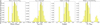 |
Fig. A.2 Histogram for fundamental parameters from rejection-sampling for 2M2244+20. |
Appendix B Silicate index definition
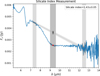 |
Fig. B.1 Example showing the windows used to define the silicate index. The JWST spectrum shown here is W0047+68. The vertical continuum windows are indicated in light grey. The silicate absorption window is highlighted in dark grey. |
All Tables
Fundamental parameters from SED analysis with updated spectral types for each object.
All Figures
|
Fig. 1 Colour-magnitude diagram indicating locations of our targets (coloured stars) at the L-T transition. The location of VHS 1256 b has also been included as a cyan circle. Planets in the HR 8799 system are also indicated as black circles. PSO J318 is indicated as a pink circle. The coral points are M dwarfs, dark red points are L dwarfs, and blue points are T dwarfs. Photometric data for each point was obtained from the Ultracool Sheet (Best et al. 2024). |
| In the text | |
|
Fig. 2 Top panel: distance-calibrated spectra for each object. Shaded regions show key absorption bands for CH4, CO, CO2, NH3 and H2O. The dotted line shows the offset level for each spectrum. The spectra are ordered by decreasing effective temperature from top to bottom. Bottom panel: cross-sections for each species, computed at T = 1300 K and P = 1 bar. |
| In the text | |
|
Fig. 3 JWST/NIRSpec Prism spectra of our sample (coloured) compared to their respective best-fitting spectral standard (black) after de-reddening (Bickle et al., in prep.). |
| In the text | |
|
Fig. 4 JWST/NIRSpec Prism NIR spectrum of 2M0642+41 (black) de-reddened and compared to L/T transition low-gravity spectral standards. The T1γ spectral standard is the best fit to 2M0642+41. The CH4 absorption regions are shaded in orange. |
| In the text | |
|
Fig. 5 Visualisation of the fundamental parameters of the sample analysed in Sanghi et al. (2023, grey circles) and our sample (coloured outlined stars). We note that Teff is plotted against the IR spectral type. The fill colour is indicative of the mass of the object. Random noise of 0.3 spectral types was added along the x-axis to minimise overlapping points in visualisation. The fundamental parameters were calculated using evolutionary models. The polynomial relations for the old field dwarfs and young moving group members (blue and red lines, respectively) from Sanghi et al. (2023) are overplotted. |
| In the text | |
|
Fig. 6 SMART fits to IGRINS spectra for W1741–46 (top) and 2M2206–42 (bottom). The grey line is the observed IGRINS spectra, the red line is the fitted model including telluric absorption, and the blue line is the fitted model without tellurics. At the bottom of each plot is the residual between the model (including tellurics) and the observed data. The shaded blue region is the ±1σ uncertainty. |
| In the text | |
|
Fig. 7 Calculated CH4 (top), H2O (middle), and silicate (bottom) indices for our sample (coloured stars) compared to those from the Spitzer IRS sample (shown as black points). The spectral types of W0047+68 and 2M2244+20 have an additional −0.15 and +0.15, respectively, for visualisation purposes. The dashed black line represents the median index for the bins of two spectral types in the Spitzer IRS sample using our updated silicate index definition in the bottom panel. |
| In the text | |
|
Fig. 8 Isolated silicate absorption features of the objects in our AB Dor sample, after continuum removal. The spectra of the silicate feature has been ordered with inclination angle, with objects viewed more equator-on towards the top and objects viewed more pole-on towards the bottom. Left panels: direct comparison of the shape of the silicate feature with the mean silicate feature of our sample (dotted black line), with the shaded region representing one standard deviation. The vertical dashed line in the left panels shows the wavelength at peak absorption for each object. Right panels: deviation from the mean silicate feature for each object. |
| In the text | |
|
Fig. 9 Correlation between the inclination and the silicate index for our sample (stars) compared with the Spitzer sample (circles) from Suárez et al. (2023). VHS 1256 b is also included with a triangle marker and black error bars. The upper panel is colour-coded according to the J-KS MKO colour anomaly calculated from young objects in the Ultracool-Sheet (Best et al. 2024). The lower panel is colour-coded according to the spectral type of each object. 2M0642+41 is not present in this figure, as it is a T dwarf with no silicate absorption feature present in the spectrum. |
| In the text | |
|
Fig. 10 Spectral comparison between Spitzer IRS observations (Suárez & Metchev 2022) and our JWST MIRI LRS observations for 2M0355+11 and 2M2244+20. The Spitzer spectra are shown in black and our spectra are coloured. Top two panels: Comparison for 2M0355+11. Bottom two panels: Comparison for 2M2244+20. The uncertainties are shown as the shaded envelope region. Below each spectral comparison is the relative flux difference (max/min − 1). |
| In the text | |
|
Fig. 11 Comparison between our objects W0047+68 and 2M2244+20 (coloured lines) and other directly imaged exoplanets: PSO J318, VHS 1256 b, and YSES-1 c (dashed, solid, and dotted black lines, respectively). For ease of comparison, the spectra of each object not included in our sample were re-normalised to match the spectral resolutions of our JWST NIRSpec Prism and MIRI LRS spectra. To highlight the 8–11 μm silicate absorption feature, each spectrum was normalised to the flux in a 0.2 μm window centred at 6.2 μm and shown in the inset. Objects in our sample are most similar to VHS 1256 b. |
| In the text | |
|
Fig. A.1 Histogram for fundamental parameters from rejection-sampling for W0047+68. |
| In the text | |
|
Fig. A.2 Histogram for fundamental parameters from rejection-sampling for 2M2244+20. |
| In the text | |
|
Fig. B.1 Example showing the windows used to define the silicate index. The JWST spectrum shown here is W0047+68. The vertical continuum windows are indicated in light grey. The silicate absorption window is highlighted in dark grey. |
| In the text | |
Current usage metrics show cumulative count of Article Views (full-text article views including HTML views, PDF and ePub downloads, according to the available data) and Abstracts Views on Vision4Press platform.
Data correspond to usage on the plateform after 2015. The current usage metrics is available 48-96 hours after online publication and is updated daily on week days.
Initial download of the metrics may take a while.