| Issue |
A&A
Volume 709, May 2026
|
|
|---|---|---|
| Article Number | A151 | |
| Number of page(s) | 19 | |
| Section | Stellar atmospheres | |
| DOI | https://doi.org/10.1051/0004-6361/202659074 | |
| Published online | 13 May 2026 | |
Reconstruction of Cepheid radial velocity curves from the shape of the V-band light curves
1
Université Côte d’Azur, Observatoire de la Côte d’Azur, CNRS, Laboratoire Lagrange,
France
2
Nicolaus Copernicus Astronomical Centre, Polish Academy of Sciences,
Bartycka 18,
00-716
Warszawa,
Poland
3
LIRA, Observatoire de Paris, Université PSL, Sorbonne Université, Université Paris Cité, CY Cergy Paris Université, CNRS,
5 place Jules Janssen,
92195
Meudon,
France
4
French-Chilean Laboratory for Astronomy, IRL 3386, CNRS,
Casilla 36-D,
Santiago,
Chile
5
Instituto de Alta Investigación, Universidad de Tarapacá,
Casilla 7D,
Arica,
Chile
6
Universidad de Concepción, Departamento Astronomía,
Casilla 160-C,
Concepción,
Chile
7
European Space Agency (ESA), ESA Office, Space Telescope Science Institute,
3700 San Martin Drive,
Baltimore,
MD
21218,
USA
8
European Southern Observatory Headquarters,
Karl-Schwarzschild-Str. 2,
85748
Garching,
Germany
★ Corresponding author: This email address is being protected from spambots. You need JavaScript enabled to view it.
Received:
22
January
2026
Accepted:
3
March
2026
Abstract
Context. Radial velocity (RV) curves of Cepheids are essential for studying their pulsation properties and also for measuring their distance via the parallax-of-pulsation method. Although precise RV curves are available for hundreds of Cepheids, it is still not possible to predict the complete RV curve from other observables such as their pulsation period or metallicity.
Aims. This paper aims to develop the first method of reconstructing the shape of the RV curves of short-period fundamental-mode Cepheids, based exclusively on their pulsation period and the morphology of their V-band light curves (LCs).
Methods. We compiled a dataset of high-quality spectroscopic and photometric measurements from the literature for 81 short-period fundamental-mode Galactic Cepheids up to a pulsation period of 8 days, enabling the precise determination of the Fourier parameters and their uncertainties. By performing a detailed comparative analysis of their shapes, we investigated correlations between LC and RV Fourier parameters and used these relations to reconstruct the RV curves. We further assessed the accuracy of these reconstructions by examining potential metallicity effects with an additional dataset of 24 metal-poor Cepheids.
Results. For pulsation periods between 3.5 and 7.0 days, we found tight correlations between different combinations of LC and RV Fourier parameters up to order 7. In particular, we discovered that the ratios R21(RV)/R21(LC) and R31(RV)/R31(LC) are tightly correlated with the pulsation period. These relationships enable the reconstruction of RV curves of Cepheids with their LC. The reconstructed curve has an uncertainty of about 0.60 km s−1 relative to the Fourier fit of true spectroscopic RV measurements. For individual Cepheids, the reconstructed RV curves integrated along the pulsation cycle (i.e. the linear radius variations) are accurate to less than 1% and precise to within 4.16% in comparison to the integrated true spectroscopic RV curves. Last, our sample of metal-poor Cepheids shows a good agreement with the empirical relations calibrated on Galactic pulsators, indicating that the method of reconstruction is weakly dependent on metallicity.
Conclusions. For the first time, we present a method of reconstructing the shape of the RV curves of Cepheids using solely the V-band LC and the pulsation period. This approach provides a valuable tool for the reconstruction of RV curves for extragalactic Cepheids through photometric data alone. It opens the road to a purely photometric parallax-of-pulsation method in the context of photometric surveys, such as the Vera Rubin Telescope. Further calibration in different photometric bands and for a larger metallicity baseline will be useful to improve the method.
Key words: methods: data analysis / methods: statistical / techniques: photometric / techniques: radial velocities / stars: variables: Cepheids
© The Authors 2026
 Open Access article, published by EDP Sciences, under the terms of the Creative Commons Attribution License (https://creativecommons.org/licenses/by/4.0), which permits unrestricted use, distribution, and reproduction in any medium, provided the original work is properly cited.
This article is published in open access under the Subscribe to Open model. This email address is being protected from spambots. You need JavaScript enabled to view it. to support open access publication.
1 Introduction
The radial velocity (RV) curves of Cepheids are essential to measure the radius variation in the application of the Baade-Wesselink (BW) method (Lindemann 1918; Baade 1926; van Hoof 1945; Wesselink 1946) for distance measurement. This technique requires high-resolution spectroscopic observations of metallic lines for accurate RV measurements (Borgniet et al. 2019), which is currently challenging to obtain for distant Cepheids beyond the Galaxy. Up to now, only a few dozen RV curves have been obtained for Cepheids in the Large and Small Magellanic Clouds (LMC and SMC) for the application of the BW method (Storm et al. 2011; Gieren et al. 2018), mostly for the brightest, long-period Cepheids, and for which the pulsation cycle is sparsely covered. The upcoming Gaia DR4 will mark a major step forward, providing RV measurements for thousands of Cepheids in the Magellanic Clouds from calcium triplet observations with the Radial Velocity Spectrometer (RVS) (Gaia Collaboration 2023; Katz et al. 2023). Despite these efforts, spectroscopic observations of extragalactic Cepheids within the Local Group remain technically challenging. To date, only two RV curves of Cepheids have been presented in a conference article, in M31 and M33, respectively (Forestell et al. 2004). For the future Extremely Large Telescope (ELT) in combination with multi-fibre instruments (Marconi et al. 2024; Pelló et al. 2024), such observations will be limited to the brightest targets and possibly a sparse coverage of the pulsation cycle.
On the other hand, RV curves of Cepheids are available for more than two hundred Cepheids in the solar neighborhood (Anderson et al. 2024; Hocdé et al. 2024, and references therein). The Fourier decompositions of these RV curves improved our understanding of their pulsation, and are also useful for various purposes, including comparison with Gaia RVS data (Anderson et al. 2024), constraining pulsation models (Paxton et al. 2019; Molinaro et al. 2025), disentangling pulsation and orbital motion (Nardetto et al. 2024; Shetye et al. 2024), and pulsation mode identification (Kienzle et al. 1999; Hocdé et al. 2024). The analysis of Cepheid RV curves through their Fourier parameters reveals a diversity of shapes and amplitudes that likely depend on the physical parameters of each star, similarly to what is observed for their LC morphologies (Bhardwaj et al. 2015; Hocdé et al. 2024).
Despite this complexity, LCs and RV curves of fundamental-mode Cepheids depend primarily on the pulsation period and their shape follows the so-called Hertzsprung progression (Ludendorff 1919; Hertzsprung 1926). This shape progression was observed among LCs of Cepheids in the Magellanic Clouds and Andromeda Galaxy (Parenago & Kukarkin 1936; Shapley & McKibben 1940; Payne-Gaposchkin 1947) and later confirmed for the RV curves (Joy 1937; Ledoux & Walraven 1958). This progression is efficiently described by Fourier decomposition of the curves (Simon & Lee 1981; Simon & Teays 1983), which can then be compared to hydrodynamical models (Buchler et al. 1990; Moskalik et al. 1992). The Hertzsprung progression is explained theoretically by the resonance between the fundamental and the second overtone pulsation modes characterized by pulsation periods of P0 and P2, respectively, as was suggested first by Simon & Schmidt (1976) and then demonstrated analytically with the amplitude equation formalism (Buchler & Kovács 1986; Kovacs & Buchler 1989). In particular, the Fourier phase difference, ϕ21, of the RV curve of the fundamental-mode depends almost exclusively on the resonant period ratio, P2/P0. The progression of this Fourier phase, both for the RV curves and for the LCs, is characterized by a pronounced discontinuity at the resonance centre at about P = 10 days. As the resonance is a dynamical phenomenon, RV curves provide information on the stellar structure and dynamics of Cepheids. On the other hand, LCs of Cepheids depend not only on the pulsation dynamics, but also on the radiative transfer through the outer layers of the photosphere.
Comparison of RV curves and LCs are rare in the literature because it demands a significant sample of stars with both well-sampled LC and RV curves. To our knowledge, only the amplitude ratio ARV/AV was studied theoretically and observationally by Balona & Stobie (1979) and Klagyivik & Szabados (2009), respectively, with the objective to better discriminate the pulsation mode of Cepheids. Understanding the link between LC and RV curves can be useful for constraining hydrodynamical pulsation models, but also to reconstruct the RV curves of Cepheids from the shape of the LCs. The objective of this paper is to propose a method of reconstructing the full RV curves of Cepheids on the basis of the V-band light curves (LCs). This new technique could be useful to complement spectroscopic observations to recover full RV curves. In the long term, the method could be combined with large-scale photometric surveys to apply the BW technique to more distant Cepheids in the Local Group, ultimately improving the calibration of the cosmic distance scale. This is particularly relevant in the framework of photometric surveys such as Gaia DR4 or the Vera C. Rubin Observatory that will obtain LCs to thousands of Cepheids (Hoffmann & Macri 2015).
In the following, we first present the calibrating sample in Sect. 2 and the calculation of Fourier parameters of LCs and RV curves in Sect. 3. We then use these parameters to fit several empirical relations between LC and RV curves in Sect. 4. In Sect. 5, we quantify the internal and external accuracy of the reconstructed shape of the RV curves, and we quantify the accuracy of the template fitting method in Sect. 6. We discuss future improvements of the method in Sect. 7 and we conclude in Sect. 8.
2 Calibrating sample
2.1 Choice of period range
In this paper, we focus on fundamental-mode Cepheids between 3 and 8 days (logP ≈ 0.48 to 0.91). In the Galaxy, this is considered to be a short-period range, while in metal-poor environments such as the LMC it might be considered as an intermediate-period range. As we calibrate our method on Galactic Cepheids, we refer to short-period Cepheids in the following. The choice of this narrow period range simplifies several aspects compared to their long-period counterparts. First, the Fourier parameters, particularly the Fourier phases of RV curves exhibit tighter and more regular progressions in this period range. This makes these stars ideal to construct a predictive method. Second, the population of Cepheids with well-sampled LC and RV curves is also larger for short-period Cepheids compared to their long-period counterparts, which also allows for a more robust study of their Fourier parameters.
Another advantage of using short-period Cepheids is due to their slower evolutionary period change of the order of 0.1 s/yr during their second and third crossing of the instability strip (Turner et al. 2006; Csörnyei et al. 2022), which largely mitigates the epoch difference between RV curves and LCs in comparison to fast evolving long-period Cepheids. We note, however, that some short-period Cepheids might undergo a fast period change because they are crossing the instability strip for the first time (Rodríguez-Segovia et al. 2022; Espinoza-Arancibia et al. 2022), but such objects are rare. Anomalously large rates of period change are also found in several Galactic Cepheids with pulsation periods below 3.5 days (Turner et al. 2006). Again, such objects are very rare and they are not represented in our calibrating sample.
Last, the 2:1 resonance at about P = 10 days introduces discontinuity in the RV and LC Fourier progressions, which are more difficult to model empirically. Therefore we limit our sample to stars with pulsation periods below 8 days. At the lower end of the pulsation period, fundamental-mode Cepheids pulsating in less than 3 days are rare in the Galaxy, contrary to what is observed for LMC and SMC Cepheids (Soszyński et al. 2008, 2010). In the following, we build a calibrating sample for short-period Cepheids between 3 and 8 days.
2.2 Source of RV curves
In this work we gather the most precise Fourier parameters for RV curves of fundamental-mode short-period Cepheids. In our recent work we provided precise Fourier parameters for 72 fundamental-mode short-period Cepheids RV curves (Hocdé et al. 2024). At the same time, new precise RV measurements were made available for 64 short-period fundamental-mode Cepheids (Anderson et al. 2024). From these two datasets, we used the best-quality fits yielding the most precise Fourier parameters. To ensure consistency in the evaluation of RV curve quality and derivation of the uncertainties, we re-computed the Fourier parameters from Anderson et al. (2024) using the method described in Hocdé et al. (2024) (see also Sect. 3). From these two samples, we selected only the stars with the best fits, based on the smallest dispersion of the fit and the absence of significant fit instabilities (labeled Quality 1 and 1a, Hocdé et al. 2024). These requirements ensure the accuracy and the precision of the Fourier parameters.
In order to complement the sample with metal-poor Cepheids, we relaxed these constraints for additional RV data. Hence, we gathered RV curves of metal-poor Cepheids observed in the LMC (Storm et al. 2011; Pilecki et al. 2018) and the SMC (Gieren et al. 2018). We also gathered Fourier parameters derived by Hocdé et al. (2024) for metal-poor Cepheids observed by Pont et al. (2001) on the outskirts of the Milky Way at a galactocentric radius of about 12–14 kpc. We included metal-poor Cepheids with pulsation period down to 2 days. This sample of stars allows the investigation of potential metallicity effect in the LMC and SMC range. However, most of the RV measurements of these stars suffer from several limitations, including a smaller number of measurements, and sparse coverage of the pulsation cycle and intrinsic scatter, both of which lead to significant instabilities in the Fourier fits. The only exceptions are the spectroscopic observations from Pilecki et al. (2013, 2018) for two LMC Cepheids with good quality data. Due to the overall poor quality of Fourier fits for metal-poor Cepheids, we decided to not include them in the calibration and to use them only to test consistency with the MW calibrating sample.
From this sample of RV curves, we selected only fundamental-mode Cepheids based on a robust pulsation mode identification using ϕ21 from the RV curve (Kienzle et al. 1999; Hocdé et al. 2024). This is particularly important for Cepheids with a pulsation period of more than 5.5 days, for which other selection criteria based on the LC shapes are ambiguous.
Our sample of RV curves consists of 81 fundamental-mode Cepheids that have a pulsation period of between 3.45 and 7.99 days (see Table A.1), with a median fit dispersion of σfit = 0.5 km/s. In a separate sample, not used for the calibration, we include 24 RV curves for metal-poor stars with a pulsation period of between 2.64 and 7.46 days listed in Table A.2. In the following, we cross-match these samples with LCs sources available in the literature.
2.3 Source of V-band light curves
The choice of the V-band LCs is motivated by several considerations. First of all, V-band LCs are available for a large number of stars, which is convenient when cross-matching with RV curves. V-band LCs are also well sampled along the pulsation cycle, which is necessary for the derivation of precise Fourier parameters. Nevertheless, extending the analysis to other photometric bands will be interesting for future work. We gathered LCs in the V band from different sources in the literature, as is presented in Table A.1. We retrieved most of the LCs sources from the compilation of Berdnikov (2008), the ASAS catalogue (Pojmanski 2002) and ASAS-SN1 (Jayasinghe et al. 2018), KISS2 (Morokuma et al. 2014), and SWASP3 (Pollacco et al. 2006). In a few cases, we complemented the data with older datasets from Moffett & Barnes (1984) and Kiss (1998). For several stars we combined these datasets to derive more precise Fourier parameters in the next section. For Cepheids of the LMC and SMC, we used mostly the LCs from OGLE4 III (Soszyński et al. 2008, 2010) and OGLE IV (Soszyński et al. 2015).
In this sample, several of the Galactic Cepheids are known binaries or member of multiple systems (Klagyivik & Szabados 2009; Evans et al. 20240; Shetye et al. 2024). In most cases the companions are main-sequence stars that are much fainter than the Cepheids (Gallenne et al. 2019). To date, V1334 Cyg is the Galactic Cepheid5 with the brightest detected companion with a flux ratio close to 10% in the V band (Evans 1995). However, other Cepheids, such as OGLE-LMC-CEP-0227, are known to have bright giant companions (Pilecki et al. 2021). For this particular star, we subtracted the light of the companion (V = 15.90 ± 0.05, Pilecki et al. 2018) in order to correct the shape of the V-band LC for this star.
Our final calibrating sample comprises 81 Cepheids with both LCs and RV curves, uniformly distributed between 3.45 and 8 days, as is shown in Fig. 1a, ensuring a consistent calibration across this period range. This sample is complemented by 24 metal-poor Cepheids from the LMC, SMC, and the outskirts of the Galaxy, which are used to verify the effect of metallicity on the empirical calibration. We cross-matched the calibrating sample with the metallicity compilation by Hocdé et al. (2023) and identified spectroscopic metallicities for 72 stars, the majority of which are from the determinations of Luck (2018). We present the histogram of the metallicities of the calibrating sample in Fig. 1b. As was expected, our calibrating sample is well centred on solar metallicity. On the other hand, the metal-poor samples (not plotted) are well centred on [Fe/H]=−0.75 dex (Romaniello et al. 2008) for SMC stars and −0.41 for LMC stars (Romaniello et al. 2022), and sub-solar values between −0.4-−0.1 for Cepheids on the outskirts of the Galaxy (Pont et al. 2001; Trentin et al. 2024).
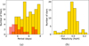 |
Fig. 1 (a) Histogram of the pulsation period of the calibrating sample in yellow and of the metal-poor sample in red. (b) Histogram of the metallicity of the calibrating sample only (see Sect. 2). |
3 Fourier parameters of LC and RV curves
3.1 Fourier decomposition
For both the LC and RV curves, we applied a Fourier fitting using the least-squares method, and computing uncertainties on the Fourier parameters following the method described by Petersen (1986). In the following, we summarize the steps of the method presented in Hocdé et al. (2024). The idea of applying Fourier expansion to periodic LCs was introduced by Schaltenbrand & Tammann (1971) and further developed by Simon & Lee (1981). For each curve, C(t), measured at time t we derived the following Fourier decomposition:
![Mathematical equation: $C(t) = {A_0} + \mathop \sum \limits_{k = 1}^n {A_k}\sin [k\omega t + {\upsilon _k}],$](/articles/aa/full_html/2026/05/aa59074-26/aa59074-26-eq1.png) (1)
(1)
where Ak and ϕk are, respectively, the amplitude and phase of the k Fourier component. Each harmonic frequency is a multiple of the fundamental frequency ω = 2π/P. The pulsation period, P, was also optimized in the fitting process. The standard deviation of the fit is given by
 (2)
(2)
where N is the number of data points, n the order of the fit, and C(ti) and Ĉi are measurements and the Fourier model, respectively. We used the standard deviation of the fit to perform 3σ clipping on the Fourier fit to remove the outliers.
To determine the order, n, of the fit, we adopted an adaptive approach, iteratively increasing n as long as the condition  was satisfied6. In some cases, one or two additional harmonics were included to stabilize the fit. The histogram of the Fourier order of RV and the LC fits for the calibrating sample is presented in Fig. 2a, which shows that RV curves require a larger number of harmonics to be described in our sample, with a median order of the fit n = 6.
For RV curves we removed possible orbital trends with secondary Fourier sum. To that effect we modelled the orbital RV with the Fourier sum with the orbital period, Porb. This method removes orbital motion as our objective is only to model the pulsational component. The only exception was for orbital motion in two LMC Cepheids, which was modeled and removed by Pilecki et al. (2018). We also corrected for possible slow linear or parabolic trends observed in residuals of LCs or RV curves, possibly due to instrumental effects or to orbital motion in the latter case. To this end we modelled the trend with a single long-period sine component with Ptrend = 50 000 days. We indicate when we corrected for such a trend in Table A.4.
Finally, we used the dimensionless Fourier parameters introduced by Simon & Lee (1981): the amplitude ratios of order k,
 (3)
(3)
and the Fourier phase difference, which locates each harmonic with respect to the first harmonic
 (4)
(4)
We present the Fourier parameters and their uncertainties obtained for both LC and RV curves in Tables A.3 and A.4, and we plot them, up to order 6, in Figs. 3a and 3b.
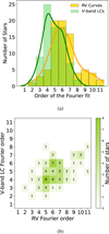 |
Fig. 2 (a) Histogram of the order of the Fourier fits for the V-band LCs and RV curves of the initial calibrating sample (81 Cepheids up to a pulsation period of 8 days). (b) 2D histogram of the LC Fourier order versus RV Fourier order. |
3.2 Effect of the pulsation period on Fourier parameters
We note that the Fourier fits yield slightly different pulsation periods for the RV curves and LCs. The difference is always smaller than 0.0003 day (about 26 seconds), as is shown in Table A.1. This discrepancy may arise from a genuine period change, since the RV and photometric data are not necessarily contemporaneous, or from numerical uncertainties in the fitting procedure. Although small, this difference can still exceed the formal uncertainty of the pulsation period. We verified that phasing of the RV data with the pulsation period derived from the LC (instead of the one derived from the RV) has only a minor effect on the RV Fourier parameters. Even for the stars exhibiting the largest difference between the two periods, the changes in velocity A1 and Rn1 never exceed the 2σ level and usually are smaller. We therefore assume in the following that the pulsation periods of the LC and RV curves are equal and we adopt the RV-derived periods for all future computations.
3.3 Qualitative description of the Fourier parameters
The qualitative trends of Fourier parameters are well documented in the literature for both V-band LCs (Soszyński et al. 2008, 2010; Bhardwaj et al. 2015; Hocdé et al. 2023000) and RV curves (Kovacs et al. 1990; Anderson et al. 2024; Hocdé et al. 2024). We observe first that the Fourier phases exhibit tight progressions with pulsation period for RV curves, while analogous progressions for the LCs are more scattered. We also confirm that there is no break in ϕ41(RV) around 7 days, contrary to what is observed for the LCs (Simon & Moffett 1985) (compare ϕ41 from Figs. 3a and 3b). The difference between ϕ41 of the RV curves and LCs was first noted by Kovacs et al. (1990), who attributed it to unknown photospheric phenomena.
Contrary to the Fourier phases, amplitude ratios display larger scatter without a noticeable trend except for R21. In the latter case, RV curves become increasingly asymmetric with the pulsation period, whereas the LCs tend towards a more symmetric profile. As an example, for the Cepheid U Vul (P=7.99 days) we derived R21(LC)=0.228, while R21(RV)=0.498, which is more than twice as large. Interestingly, this apparent opposite behaviour of LCs and RV curves is already visible from pulsation models (see Figure 6 in Moskalik et al. (1992), and more recently Paxton et al. (2019)). These effects are caused by the difference in the behavior of the second harmonic, A2, since the amplitudes A1(RV) and A1(LC) are scattered in Fig. 4, showing no particular trend with the pulsation period. This is clearly visible for the calibrating sample of the Galactic Cepheids (yellow and green symbols).
Several studies have examined empirically the impact of metallicity on the LC shapes of Cepheids (Antonello et al. 2000; Klagyivik & Szabados 2007; Szabados & Klagyivik 2012; Majaess et al. 2013; Klagyivik et al. 2013; Bhardwaj et al. 2015; Hocdé et al. 2023). In the case of the short-period Cepheids, the most significant effects are observed in R21 and R31, which are higher for metal-poor Cepheids, with tight empirical correlations (Klagyivik et al. 2013; Hocdé et al. 2023). For RV curves, Pont et al. (2001) found that metal-poor Cepheids with periods below 5 days show larger values of A1 and R21, while ϕ21 remains unaffected. We confirm these trends using a sample of metal-poor Cepheids twice as large, after the inclusion of the RV curves of the LMC and SMC stars (see red error bars in Figs. 3a and 4). We also observe a prominent peak in the amplitude ratios at around 4 days for both LCs and RVs of metal-poor Cepheids. Moreover, we show for the first time that this effect is persistent for amplitude ratios up to the seventh order, while the Fourier phases remain unaffected.
These qualitative descriptions highlight the influence of both the pulsation period and metallicity on the shape of the RV curves in short-period Cepheids. The clear and regular progression of the RV Fourier phases makes them easier to model as a function of the pulsation period. In contrast, the significant scatter and the apparent discrepancies between R21 of LCs and RV curves motivate us to investigate potential correlations between them, with particular attention paid to the role of metallicity.
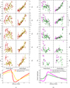 |
Fig. 3 Fourier amplitude ratios and phase parameters (R21 to R61 and ϕ21 to ϕ61) of Cepheid RV curves (a) and LCs (b) as a function of the period. Models for MU Cep and OGLE-LMC-CEP-227 are shown to illustrate the difference between solar and sub-solar metallicity around P = 4 day. The solar and sub-solar metallicity variables are plotted with yellow and red error bars (magenta and green, respectively) for the RV curves (LCs, respectively). Fourier parameters are derived with decomposition analysis presented in Sect. 3. |
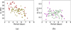 |
Fig. 4 Amplitude of the first harmonic, A1, for RV curves (a) and for LCs (b). Cepheids of solar metallicity are plotted with yellow and green symbols and those of sub-solar metallicity with red and magenta symbols. |
4 Reconstruction of RV curves from the LC shapes
4.1 Empirical relations
In order to reconstruct the RV curves of Cepheids, we need to infer the Fourier parameters of these RV curves. This is straightforward in the case of the Fourier phase differences, since these parameters follow a well-defined relation with the pulsation period. For the amplitudes and amplitude ratios of the RV curves, we explored possible correlations with the Fourier parameters of the LCs. Specifically, we first visually inspected various combinations of Rk1(RV) as a function of Rk1(LC) and the pulsation period, and A1(RV) as a function of A1(LC) or Rk1(LC). As a result, we found several empirical relations up to order seven for amplitude ratios and phase differences, as is presented in Fig. 5, and for the amplitude, A1, in Fig. 6. In many of these empirical relations, we observe a break at a period of 7 days. For this reason we restrict our subsequent analysis to Cepheids with P < 7 day and omit the ones with longer periods (plotted with grey symbols in Figs. 5 and 6).
In order to model the different correlations, we chose a simple approach of fitting either linear relations of the form
 (5)
(5)
or a power law,
 (6)
(6)
For all relations between different Fourier parameters, we applied orthogonal distance regression (ODR) to properly account for uncertainties in both the dependent and independent variables. This method minimizes the orthogonal distances between data points and the fitted model, thereby incorporating errors in both variables. We utilized the ODR implementation provided by the SciPy library7. For the empirical relations depending on the pulsation period, we employed a standard nonlinear least-squares fitting, using the curve_fit function8 from Python, considering only the uncertainties in the dependent variable. We display the fitted relations with blue lines in Figs. 5 and 6 and we provide the coefficients with statistical errors, reduced  and RMS of the fits in Table 1.
As was expected, phase differences correlate well with the pulsation period, as we can see from Figs. 5a–5f. For the amplitude ratios we discovered a progression of the ratio of amplitude ratios, R21(RV)/R21(LC), with the pulsation period, and similarly for R31(RV)/R31(LC) (see Figs. 5g and 5h). This result contrasts with the apparent large scatter of R21 and R31 described in the previous section, and shows that the shape of both the LCs and RV curves follows empirical correlations with the pulsation period. Furthermore, we find that all higher-order Rk1(RV) parameters correlate well with R21(LC) up to order seven (see Figs. 5i–5l). Last, A1(RV) correlates with R21(LC), R31(LC), and a combination of both (see Figs. 6a–6c).
4.2 Metallicity dependence
For all these empirical relations, we overplot Fourier parameters of metal-poor Cepheids in red in Figs. 5 and 6. These Fourier parameters were derived from RV curves of much lower quality, and thus must be interpreted with caution. Despite the lower accuracy, we found that metal-poor Cepheids closely follow the empirical relations R21(RV)/R21(LC) and R31(RV)/R31(LC) between 3.5 and 7 days, with the exception of two outliers (OGLE-LMC-1327 and 1249).
We also find that the A1(RV) coefficient of metal-poor Cepheids very closely follows the linear correlation with R21(LC), R31(LC), or a combination of both, defined by our calibrating sample (see Fig. 6). Despite larger error bars, we also see that the higher-order amplitude ratios of metal-poor Cepheids follow the trend of our calibrating sample. Although the lower precision of the Fourier parameters of metal-poor RV curves, combined with the limited size of the sample, prevents us from making a firm conclusion, our results indicate that the empirical relations presented in this paper do not depend strongly on the metallicity.
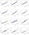 |
Fig. 5 Fourier parameters of RV curves as a function of pulsation period and V-band LC shape: (a) ϕ21, (b) ϕ31, (c) ϕ41, (d) ϕ51, (e) ϕ61, (f) ϕ71, (g) R21, (h) R31, (i) R41, (j) R51, (k) R61, (l) R71. Yellow circles (calibrating sample) are used to produce the fits between 3.45 and 7 days (blue lines, see Sect. 4); red circles show metal-poor Cepheids; grey points above P > 7 days are ignored in the fit; violet points are metal-poor Cepheid outside the pulsation period range 3.4 to 7 days. |
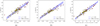 |
Fig. 6 Fourier parameter A1 of the RV curves as a function of (a) R21(LC), (b) R31(LC), and (c) a combination of R21(LC) and R31(LC). The ODR fit (blue line) was applied to the calibrating sample (yellow circles) and prolongated to show consistency with metal-poor stars (red circles). |
Empirical relations for the Fourier phases, ϕk1(RV), and amplitude ratios, Rk1(RV), as functions of the pulsation period, P, or LC Fourier parameters, R21 and R31.
4.3 Reconstruction method
With the empirical relations established in the previous section, it is possible to reconstruct the RV curve of a given Cepheid using the Fourier parameters of the V-band LC and the pulsation period. Fourier phase differences, ϕk1(RV), up to order 7 can be determined knowing the pulsation period only. Fixing arbitrarily ϕ1 = 0, we are then able to unfold all phases ϕk>1(RV) using Eq. (4) and fitted relations in Table 1. On the other hand, the amplitude ratios R21(LC) and R31(LC) of the V-band LC allow one to determine the amplitude ratios of the RV curves, Rk1(RV), up to order 7 as well as the amplitude of the first harmonic, A1(RV). We adopted the A1 relation as a function of the combination of R21(LC) and R31(LC), as it provides the smaller RMS with 0.577 km/s. Then, we deduce the amplitudes of all the remaining harmonic since Ak = A1Rk1. As a result, we can sum up all the harmonics to reconstruct the RV curves’  following
![Mathematical equation: $V_r^{rec}(t) = \mathop \sum \limits_{k = 1}^n {A_k}\sin [k\omega t + {\phi _k}].$](/articles/aa/full_html/2026/05/aa59074-26/aa59074-26-eq12.png) (7)
(7)
Analysing the accuracy of reconstruction for different orders of the Fourier fit, we determined n = 6 as the optimal order for our calibrating sample. This analysis is presented in Sect. 5.3. We provide examples in Fig. 7 of reconstructed RV curves for several Cepheids of the calibrating sample, and in Fig. 8 for lower-quality metal-poor Cepheids. The entire set of reconstructed RV curves is available online on zenodo. The Cepheid CR Cep was rejected from this reconstruction because its LC was modeled with the Fourier fit of the order two, and thus it was not possible to use the R31(RV)/R31(LC) relation.
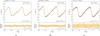 |
Fig. 7 Examples of reconstructed RV curves of excellent, medium, and lower accuracy in the case of (a) CS Mon, (b) AP Sgr, and (c) Y Lac, respectively. The yellow curve shows the reconstructed RV curve using empirical relations defined in Table 1; the black curve is the Fourier fit to the RV observations (red points, see Table A.1). The accuracy of the reconstructed RV curve is defined by the standard deviation of the residuals along the pulsation cycle. |
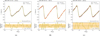 |
Fig. 8 Examples of reconstructed metal-poor RV curves of good, medium, and lower accuracy for the Cepheids (a) OGLE-SMC-1717, (b) OGLE-LMC-227, and (c) OGLE-LMC-1249. The black curve is the Fourier fit to the RV observations (red points, see Table A.2). |
5 Accuracy of the reconstructed RV curves
In this section, we first estimate the internal accuracy of the reconstructed shape of the RV curves of the calibrating sample, which serve as indicators of the fit quality. We then estimate realistic external accuracy with a Monte Carlo resampling, which enables us to assess how well our method generalizes to stars outside the calibrating sample.
5.1 Reconstruction residuals
Our objective is to assess the precision of the reconstructed RV curves with respect to the real RV curves. To this end, our strategy is to compare the RV reconstruction for each star with its RV Fourier fit, defined by the true spectroscopic measurements. This is possible and reliable because the Fourier fits for Cepheids of the calibration sample are of excellent quality and do not have any significant instabilities (Hocdé et al. 2024). However, the RV curves of metal-poor Cepheids are not suitable for this comparison because of lower-quality fits. Nevertheless, we decided to perform this calculation for metal-poor Cepheids as well, but these results must be treated with caution.
Hence, we compared for each star the reconstructed RV curve,  , with the Fourier fit of the true RV curve,
  . This was done by deriving the root mean square of the residuals,
 (8)
(8)
which is a measure of internal accuracy of the reconstructed RV curve. Since  and
and  have arbitrary phasing, we chose the phase of
  in such way as to minimize the residuals, σrms(Vr). The two curves were sampled at N = 100 regularly spaced phases along the pulsation cycle. The resulting reconstruction residuals for individual stars are plotted against the pulsation period in Fig. 9a. Overall, we find a median σrms = 0.53 km/s for the calibrating sample (see dashed orange line in Fig. 9a), which shows the excellent precision of the reconstructed RV curves. From Fig. 9a, we do not find any trends with the pulsation period. For several stars, the accuracy is even better than 0.5 km/s, as we can see for example in the case of CS Mon in Fig. 7a with σrms = 0.44 km/s. This result is particularly remarkable given that only information on the LC and the pulsation period was used to reconstruct the RV curves.
On the other hand, five stars have reconstruction residuals of 1 km/s or more: AW Per, FM Aql, Y Lac, SS Sct, and CS Ori. This is most likely caused by a mismatch of the amplitudes, as in the case of Y Lac (see Fig. 7c), because all these stars except for AW Per are outliers of the A1 relation (see Fig. 6c). At this stage, we do not have a clear explanation for the origin of the A1(RV) outliers. We note, however, that the derived empirical relations for A1 are highly sensitive to the LC amplitude ratios, R21 and R31. Consequently, small errors in the numerical determination of these parameters, or photometric contamination of the LC, could bias the estimation of A1. According to our calibration, an offset as small as ∆R21(LC) = 0.035 can bias A1(RV) by about 1 kms−1.
It is well known that blending with a bright companion or crowding can bias both the mean brightness and the LC amplitude (Mochejska et al. 2000; Klagyivik & Szabados 2009). Several Cepheids in our sample are known binaries (Klagyivik & Szabados 2009; Shetye et al. 2024). Among five objects with reconstruction residuals above 1km/s, binarity is well established for AW Per Evans et al. (2024) and has been suggested for CS Ori (Szabados & Pont 1998). The presence of a photometric companion has also been claimed in the case of Y Lac (Evans et al. 1990).
However, we emphasize that blending has a relatively small effect on the LC amplitude ratios, as was shown by Antonello (2002): a strong blending of about 0.45 mag, equivalent to 50% of the Cepheid luminosity, is required to increase R21 by only 0.02 (see their Figure 2). Although such bright companions can exist, we know from analysis of the PL relation that they are rare (Pilecki et al. 2021). Another possible source of photometric contamination could arise from circumstellar emission during the pulsation cycle in the V band (Hocdé et al. 2020b,a).
As was expected, the reconstruction of the RV curves for metal-poor Cepheids yields significantly larger residuals than for the calibrating Cepheids, with a median of σrms = 1.09 km/s (see red crosses in Fig. 9a). We emphasize that in most of our metal-poor Cepheids, the Fourier fits to the true spectroscopic RV curves are of lower quality and as such they are not accurate enough to properly assess the uncertainties of the reconstruction method. Despite this shortcoming, for several metal-poor Cepheids the reconstructed RV curves differ by less than 1 km/s from the true RV curves (XX Mon, BC Pup, OGLE-SMC-1680, and OGLE-SMC-1717 also presented in Fig. 8a).
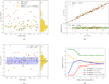 |
Fig. 9 Internal accuracy of reconstructed RV curves for calibrating Cepheids and for metal-poor Cepheids (yellow circles and red crosses, respectively). (a) Reconstruction residuals, σrms(Vr), for individual stars, as defined by Eq. (8). The dashed orange line indicates the median of the residuals for the calibrating sample. (b) Comparison of absolute integrated RV curves, as defined in Eq. (9). In the lower panel, we plot the differences between the two values. The dashed red line indicates the median of the differences, with the shaded green area marking their RMS. (c) Relative peak-to-peak amplitude difference between the reconstructed RV curves and true RV curves (Fourier fits), as defined in Eq. (10). The dashed blue line indicates the median value for the calibrating sample. (d) Accuracy of the RV curve reconstruction for Cepheids of the calibrating sample, versus the Fourier order (see also Table 2). The different lines represent the four previously discussed measures of accuracy, plotted with the same colours as in Figs. 9a–c (see Sect. 5.3). |
5.2 Accuracy of the integrated RV curves
The accuracy of the integrated RV curve is a key factor in the BW method (Nardetto et al. 2004; Marengo et al. 2004). In Fig. 9b, we compare the integrated RV curves obtained with the reconstruction and the true ones, derived with the spectroscopic RV data (Fourier fits). To this end, we computed the integrated absolute value of the RV curves along the pulsation cycle, which is equivalent to the total linear radius variation, ∆R, normalized by the projection factor9, p:
 (9)
(9)
The differences between ∆R/p computed from reconstructed RV curves and from the true RV curves (Fourier fits) has a standard deviation of 4.16%. This error must be accounted for in the BW method, as it propagates directly into the error budget of the derived distances (Marengo et al. 2004). Nevertheless, the median difference of the total integrated RV curves remains below 1% at −0.57%. This result is crucial for application of the BW method based on RV curve reconstruction. Indeed, while individual stars may carry uncertainty of a few percent, the integrated reconstructed RV curve averaged over a Cepheid population of 59 stars is accurate to better than 1%. Somewhat surprisingly, the integrated RV curves of metal-poor Cepheids also show a good performance, with a slightly larger dispersion of 6.96% and a median difference of 2.00% with respect to their Fourier fit. We deduce that the integrated RV curves of Cepheids are not very sensitive to the fit instabilities and high-order errors. We conclude that the integrated reconstructed RV curves of Cepheids, when used in the context of the BW method over a sample of a large number of stars, induce for solar-metallicity Cepheids (metal-poor Cepheids, respectively) systematics no larger than 1% (2.0%, respectively), with a statistical precision of better than 5% (7%, respectively).
We also derived the relative difference of peak-to-peak amplitudes between the reconstructed RV curves and the true RV curves (Fourier fits):
 (10)
(10)
Within our sample, we find that the median of the relative difference of amplitudes is smaller than 1% (see dashed blue line in Fig. 9c) with a dispersion of about 5% (see blue area in Fig. 9c). We do not find significant trend within the sample. As in the case of the previously discussed indicators, the metal-poor Cepheids with low-quality RV fits show a higher dispersion (7.24%) and higher median (3.57%) of the relative amplitude difference, ∆Ap2p/Ap2p.
5.3 Optimal order of reconstruction
From the histogram of the order of the Fourier fits (Fig. 2a), we see that most of the RV curves are modelled with fits of the order of between 5 and 7, with a median of n = 6. For pulsation periods below 7 days, 48 out of 59 stars of our calibrating sample (i.e. 83%) have Fourier fits of order n ≤ 7, while fits of the order of between 5 and 7 are used in 42 stars (71%). These results are comparable with the median order of the fit determined for the short-period Cepheid sample (n = 7, 47 stars) of Anderson et al. (2024). However, the order of the fit is sensitive to the stellar properties such as the amplitude and the pulsation period, but also to the quality of the data such as the accuracy of the measurements, number of data points and the phase coverage.
To reconstruct the shape of RV curve of a Cepheid, we first have to decide what Fourier order should be used. Unfortunately, we did not find a way to determine the order of the RV fit, for example as a function of the order of the LC fit and the pulsation period. This is so because of a poor correlation between the fit order of the RV curves and of the LCs, as we can see in Fig. 2b. Instead, we chose to find the order that will be optimal for reconstructing the RV curves for all Cepheids of the calibrating sample. To this end, we reconstructed the RV curves of the calibrating sample using different orders from n = 1 to n = 7, and then for each reconstruction we computed different measures of accuracy:
the median of RV reconstruction residuals, σrms(Vr), as defined by Eq. (8) and plotted in Fig. 9a,
the RMS of differences and the median bias of the absolute integrated RV curves, as plotted in Fig. 9b,
and the median of relative amplitude difference, ∆Ap2p/Ap2p, as presented in Fig. 9c.
We plot the result in Fig. 9d (see also Table 2). Overall, the quality of the reconstruction improves rapidly up to order 3, and the addition of higher orders has only a small, yet non-negligible, effect on the accuracy of the reconstruction. We find that a fit of the order of n=5–7 is optimal for reconstruction of RV curves in the calibrating sample, because it minimizes all four measures of accuracy. We decided to use n=6 as our final choice. This is the same values as the median order of the fit for the calibrating sample.
Therefore, our reconstruction overestimates the fit order of about one third of the calibrating sample (order strictly below 6, 19 stars out of 59) and underestimates the fit order for 42% of the sample (25 out of 59). Neglecting orders higher than 6 has a negligible impact on the reconstruction quality, because the amplitudes of higher-order harmonics constitute less than 5% of the amplitude of the first harmonic (see for example R71 in Fig. 5l).
However, the error introduced could be larger in the case of RV curves with a low fit order. This effect is largely mitigated by the fact that only 10% of stars in the calibrating sample have a fit order strictly below 5, so the number of Cepheids for which the fit error might be larger remains limited. Besides, the Cepheids with an order of the fit of 4 or less, namely CF Cas (σrms = 0.68 km/s), V1154 Cyg (σrms = 0.36 km/s), V1162 Aql (σrms = 0.79 km/s), V733 Aql (σrms = 0.72 km/s), and V496 Aql (σrms = 0.61 km/s), usually do not have significant errors, except for SS Sct (σrms = 1.12 km/s). This can be explained by the fact that RV curves modelled with low-order Fourier fits usually have lower amplitudes and consequently lower amplitude ratios. Therefore, higher Fourier orders contribute less to the overall error of the reconstruction. In conclusion, while individual determination of the fit order is desirable for the most optimal reconstruction of individual stars, we are confident that fixing the order of the fit at n = 6 is sufficient for most of the Cepheids.
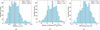 |
Fig. 10 External accuracy of the reconstructed RV curves from Monte Carlo resampling (see Sect. 5.4). In each plot, the dashed red line indicates the median of the distribution. (a) Reconstruction residuals, σrms(Vr), as defined by Eq. (8). (b) Difference between the absolute integrated RV curves (see Eq. (9)), computed from the reconstructed and from the true RV data. (c) Relative peak-to-peak amplitude difference between the reconstructed RV curves and true RV curves (Fourier fits), as defined in Eq. (10). |
Accuracy of the reconstructed RV curves’ shape as a function of the Fourier fit order.
5.4 Monte Carlo cross-validation
To assess realistic external accuracy and the generalization capability of our method, we applied a bootstrapping approach. In each realization, we randomly selected 20% of the stars from the calibrating sample (12 stars), while the remaining 47 stars form the training set. This procedure was repeated 500 times with different random realizations of the test sample. External accuracies were derived from the reconstruction residuals obtained for each test subset, following the same procedure as for the previous measurements. The median of reconstruction residuals provides a realistic estimate of the overall performance and predictive power of our method. The result of the Monte Carlo procedure is presented in Fig. 10. We obtain results that are consistent with the overall accuracy of our calibration. We show that our method is able to reconstruct external RV curves with a median accuracy of 0.60 km/s as compared to the Fourier fits of true spectroscopic RV measurements (see Fig. 10a). The absolute integrated RV curves are also accurate, with a median difference of only −0.16 with respect to the true RV curves (see Fig. 10b).
6 Template fitting method
In the previous section, we demonstrated the ability of our method to precisely reconstruct the shape of the RV curves of Cepheids. We now estimate the accuracy of this technique as a template fitting method. Indeed, given the few RV measurements available for a Cepheid, it is possible to adjust the phase and the systemic velocity in order to fit the RV model obtained from the shape of the LC. In order to test these templates, we used the same training and test samples as were generated for the bootstrapping method presented in Sect. 5.4. For each star in the validation sample, we selected 3, 4, 5, 6, and 7 RV measurements from the initial dataset presented in Sect. 2.2. These RV measurements were selected to be uniformly distributed along the pulsation cycle, starting from a random pulsation phase for each star. This procedure allowed us to avoid as much as possible any co-linear points that were not able to constrain the template fitting. While a spectroscopic survey may not ensure a regular cadence of observation, our method ensures robust accuracy determination in optimal conditions. For each sample of RV measurements, we arbitrarily offset the phase and the systemic velocity. We then used the RV model derived from the shape of the LCs as determined by the training set, and we applied a least-squares method to adjust the phase and vγ in order to fit the RV measurements. The results for 3, 4, and 5 RV measurements are presented in Fig. 11 and for 3–7 RV measurements in Table 3 and Fig. 12.
Our results show that with only three RV measurements regularly spaced along the pulsation cycle, our templates are capable of fitting the RV measurements with a median uncertainty of 0.7 km/s with respect to the true Fourier fit on the available RV data. This accuracy improves with the number of RV measurements. The systemic velocity was also determined accurately, to better than 30 m/s, with a typical precision of a few 100 m/s, depending on the number of RV measurements used to fit the templates.
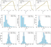 |
Fig. 11 Template fitting accuracy for 3, 4, and 5 RV measurements in each column, respectively. The first row, (a–c), displays an example of template fitting for three different stars. The second row, (d–f), presents template accuracy with respect to the Fourier fit (true RV curve) obtained from bootstrapping method on the test sets. The last row, (g–i), presents the difference in systemic velocity from each template fitting with respect to the true value, also presented in Table 3. |
Accuracy of the template fitting.
7 Discussion
7.1 Calibration of the phase lag between LC and RV curves
In this paper, we proposed a method of reconstructing the shape of the RV curves. However, we are not yet able to accurately phase the RV curves with respect to the LC as we have no information on the phase difference between the two. In order to reconstruct the RV curves with proper phases, it is necessary to derive this phase difference, also called the phase lag, defined as ∆ϕ1 = ϕ1(RV) − ϕ1(LC), with ϕ1 being the phase of the first harmonic. The values of the phase lag were measured for a sample of Galactic fundamental-mode Cepheids by Ogłoza et al. (2000), who found a mean value of ∆ϕ1 = −0.28 ± 0.10 rad, independent of the pulsation period, for a sample of Galactic Cepheids. To illustrate the range of values for ∆ϕ1, we display in Fig. 13 an example of RV curve reconstruction for δ Cep, phased with respect to the LC using ∆ϕ1 = −0.28 ± 0.10. As we can see, an uncertainty of ∆ϕ1 of only 0.2 rad translates to an uncertainty in the pulsation phase of only δϕ = 0.03. This narrow range can be useful to constrain the phasing of the reconstructed RV curves for application of the BW method.
However, a note of caution is necessary. Szabó et al. (2007) showed theoretically that the phase lag depends on the mass-luminosity relation and possibly also weakly on the metallicity of the Cepheids. Therefore, while the range of ∆ϕ1 determined by Ogłoza et al. (2000) can in principle be used for constraining relative phases of RV curves and LCs, a more precise calibration is needed, focusing on the pulsation period range of our method. We shall address this topic in a paper in preparation.
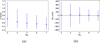 |
Fig. 12 Accuracy of the template fitting method as a function of the number of RV measurements. (a) RMS of the residual between fitting and template and the Fourier fit of the true RV curves. (b) Difference of systemic velocity. |
 |
Fig. 13 LC and reconstructed RV curve of δ Cep using phase lag range derived by Ogłoza et al. (2000). The grey zone represents the possible location of the RV curve. |
7.2 Limitations and improvements
The method presented in this paper shows that it is possible to reconstruct the RV curves of Cepheids with reasonable precision. Several aspects can, however, be improved in the future in order to perform the reconstruction with even higher precision. We have shown in this paper the good agreement of the metal-poor Cepheids with our calibrating sample, but only precise measurements will make it possible to investigate the metal dependency in more detail. Thus it is important to increase the effort of spectroscopic observations of metal-poor Cepheids, particularly with P ∼ 4 days, which exhibit much larger amplitudes and amplitude ratios. RV measurements utilizing the calcium triplet of LMC and SMC Cepheids from Gaia DR4 will be also useful for comparison with our reconstructed RV curves.
Another source of uncertainty is a possible secular or irregular period change during the Cepheid evolution (Csörnyei et al. 2022; Rathour et al. 2025). Since our calibrating sample consists of RV curves and LCs that were not obtained at the same epoch, a part of the dispersion of the empirical relations between their Fourier parameters might be caused by this effect. Therefore, simultaneous observations of both the LC and the RV curves would certainly improve the calibration.
Extending the RV reconstruction method to other photometric bands will be important in order to apply the method to different photometric surveys. It is particularly relevant to calibrate our empirical relations directly into the Sloan bands, which are used by the Vera Rubin Telescope. Moreover, while our work focuses only on short-period Cepheids between 3 and 7 days, extending the method to long-period Cepheids could be useful for reconstructing RV curves of more distant extragalactic Cepheids. Our method could be also calibrated using Gaia LCs and RVs.
7.3 Toward extrinsic RV curve templates
Up to now, templates for RV curves remain intrinsic, i.e. a Fourier fit for a given star was used to fit a few RV measurements obtained at different epochs. This method was used for the determination of the systemic velocity induced by the orbital motion (Anderson et al. 2016; Anderson 2019; Nardetto et al. 2024; Shetye et al. 2024). On the contrary, there are no extrinsic template fitting methods that allow one to determine the mean velocity of Cepheids without a priori knowledge of their RV curves. Such templates are already mature in the case of LCs (Inno et al. 2015; Bras et al. 2025), allowing one to determine the mean magnitude of extragalactic Cepheids in different bands. Our reconstruction method, on the other hand, could be useful for this purpose for any short-period Cepheids for which the V-band LC is available. This opens the possibility of detecting orbital motion for a larger number of Cepheids, while reducing the number of required spectroscopic (RV) observations. Alternatively, our reconstructions could be used for template-fitting to complement high-resolution spectroscopic observations in the context of the BW method.
7.4 Toward a photometric BW method
Apart from the systematic errors linked to the projection factor (Trahin et al. 2021; Nardetto et al. 2023), the application of the BW method remains limited by the difficulty of obtaining high-precision RV measurements for a statistically significant sample of extragalactic Cepheids. A new generation of spectroscopic instruments, ANDES and MOSAIC of the ELT, will enable us to obtain RV curves of Cepheids in the Local Group (Roederer et al. 2024; Marconi et al. 2024; Pelló et al. 2024). However it will either be expensive to obtain RV measurements that cover the pulsation cycle with limited telescope time, or beyond the capability of those instruments, which will be limited to mAB = 20 mag for integration times of ∼ 1 h.
In contrast, the method presented in this paper is easily applicable to thousands of Cepheids from galaxies of the Local Group thanks to their LCs. In combination with angular diameter measurements from precisely calibrated surface brightness-colour relations (Bailleul et al. 2025), this opens the possibility of a new purely photometric BW method. This is particularly relevant in the era of photometric surveys, such as the Vera Rubin Telescope, which will be able to obtain excellent phase coverage for Cepheids down to P = 4 days, located in galaxies as distant as 4.4 Mpc (Hoffmann & Macri 2015). In principle, well-covered LCs with a minimum of 30–35 data points are enough to obtain accurate estimations of their pulsation periods and their Fourier parameters, R21 and R31, which are the only information necessary to reconstruct the shape of the RV curves. Besides, our method is almost insensitive to blending and to the metallicity of Cepheids. In our next paper (in preparation), we show the potential to determine LMC and SMC distances and evaluate the level of systematics of a purely photometric BW method.
8 Conclusion
In this paper, we calibrated a new method that allows one to reconstruct the shape of the RV curves of fundamental-mode classical Cepheids using only the pulsation periods and the Fourier parameters R21 and R31, of their V-band LCs. This new approach to RV curve reconstruction is useful for understanding the relation between LC and RV curves, which in turn can help to constrain Cepheid hydrodynamical models. We show that our method is able to reconstruct the shape of RV curves with a precision of 0.60 km/s compared to the true RV curves determined with the spectroscopic measurements. For the sample of Cepheids, the integrated reconstructed RV curves (which are equivalent to ∆R/p) are accurate on average to better than 1% and precise to better than 5%. The high accuracy and precision of the reconstruction makes the method ideal to apply it to a BW analysis of a statistically large sample of Cepheids. Future work will be useful to reduce the scatter of the empirical calibrations, establish the calibrations in different photometric bands, and extend the range of pulsation periods.
Data availability
Full Tables of Fourier parameters A.3 and A.4 are available at the CDS via https://cdsarc.cds.unistra.fr/viz-bin/cat/J/A+A/709/A151. Figures of RV reconstruction of the calibration sample and the metal-poor Cepheids are available at https://zenodo.org/records/19061798.
Acknowledgements
The authors acknowledge the support of the French Agence Nationale de la Recherche (ANR), under grant ANR-23-CE31-0009-01 (Unlockpfactor). B.P. gratefully acknowledges financial support from the Polish National Science Centre grant SONATA BIS 2020/38/E/ST9/00486. R.S. acknowledges support from the SONATA BIS grant, 2018/30/E/ST9/00598, from the National Science Center, Poland. We also acknowledge support from the Polish Ministry of Science and Higher Education grant 2024/WK/02. The research leading to these results has received funding from the European Research Council (ERC) under the European Union’s Horizon 2020 research and innovation program (projects CepBin, grant agreement 695099, and UniverScale, grant agreement 951549). AG acknowledges the support of the Agencia Nacional de Investigación Científica y Desarrollo (ANID) through the FONDECYT Regular grant 1241073. We acknowledge with thanks the variable star observations from the AAVSO International Database contributed by observers worldwide and used in this research. This research made use of the SIMBAD and VIZIER databases at CDS, Strasbourg (France) and the electronic bibliography maintained by the NASA/ADS system. This research also made use of Astropy, a community-developed core Python package for Astronomy (Astropy Collaboration 2018, 2022).
References
- Anderson, R. I. 2019, A&A, 623, A146 [NASA ADS] [CrossRef] [EDP Sciences] [Google Scholar]
- Anderson, R. I., Casertano, S., Riess, A. G., et al. 2016, ApJS, 226, 18 [NASA ADS] [CrossRef] [Google Scholar]
- Anderson, R. I., Viviani, G., Shetye, S. S., et al. 2024, A&A, 686, A177 [NASA ADS] [CrossRef] [EDP Sciences] [Google Scholar]
- Antonello, E. 2002, A&A, 391, 795 [NASA ADS] [CrossRef] [EDP Sciences] [Google Scholar]
- Antonello, E., Fugazza, D., & Mantegazza, L. 2000, A&A, 356, L37 [NASA ADS] [Google Scholar]
- Astropy Collaboration (Price-Whelan, A. M., et al.) 2018, AJ, 156, 123 [Google Scholar]
- Astropy Collaboration (Price-Whelan, A. M., et al.) 2022, ApJ, 935, 167 [NASA ADS] [CrossRef] [Google Scholar]
- Baade, W. 1926, Astron. Nachr., 228, 359 [NASA ADS] [CrossRef] [Google Scholar]
- Bailleul, M. C., Nardetto, N., Hocdé, V., et al. 2025, A&A, 698, A46 [NASA ADS] [CrossRef] [EDP Sciences] [Google Scholar]
- Balona, L. A., & Stobie, R. S. 1979, MNRAS, 189, 649 [NASA ADS] [Google Scholar]
- Barnes, T. G., III, Fernley, J. A., Frueh, M. L., et al. 1997, PASP, 109, 645 [NASA ADS] [CrossRef] [Google Scholar]
- Berdnikov, L. N. 2008, VizieR Online Data Catalog: II/285 [Google Scholar]
- Berdnikov, L. N., Kniazev, A. Y., Sefako, R., et al. 2015, Astron. Lett., 41, 23 [Google Scholar]
- Bhardwaj, A., Kanbur, S. M., Singh, H. P., Macri, L. M., & Ngeow, C.-C. 2015, MNRAS, 447, 3342 [CrossRef] [Google Scholar]
- Borgniet, S., Kervella, P., Nardetto, N., et al. 2019, A&A, 631, A37 [NASA ADS] [CrossRef] [EDP Sciences] [Google Scholar]
- Bras, G., Kervella, P., Mérand, A., et al. 2025, A&A, 698, A97 [NASA ADS] [CrossRef] [EDP Sciences] [Google Scholar]
- Buchler, J. R., & Kovács, G. 1986, ApJ, 303, 749 [NASA ADS] [CrossRef] [Google Scholar]
- Buchler, J. R., Moskalik, P., & Kovacs, G. 1990, ApJ, 351, 617 [NASA ADS] [CrossRef] [Google Scholar]
- Csörnyei, G., Szabados, L., Molnár, L., et al. 2022, MNRAS, 511, 2125 [CrossRef] [Google Scholar]
- Espinoza-Arancibia, F., Catelan, M., Hajdu, G., et al. 2022, MNRAS, 517, 1538 [Google Scholar]
- Evans, N. R. 1995, ApJ, 445, 393 [NASA ADS] [CrossRef] [Google Scholar]
- Evans, N. R., Szabados, L., & Udalska, J. 1990, PASP, 102, 981 [NASA ADS] [CrossRef] [Google Scholar]
- Evans, N. R., Gallenne, A., Kervella, P., et al. 2024, ApJ, 972, 145 [NASA ADS] [CrossRef] [Google Scholar]
- Forestell, A. D., Barnes, T. G., III, Sneden, C., & Moffett, T. J. 2004, in Astronomical Society of the Pacific Conference Series, 310, IAU Colloquium 193: Variable Stars in the Local Group, eds. D. W. Kurtz, & K. R. Pollard, 99 [Google Scholar]
- Gaia Collaboration (Vallenari, A., et al.) 2023, A&A, 674, A1 [NASA ADS] [CrossRef] [EDP Sciences] [Google Scholar]
- Gallenne, A., Kervella, P., Borgniet, S., et al. 2019, A&A, 622, A164 [NASA ADS] [CrossRef] [EDP Sciences] [Google Scholar]
- Gieren, W. P., Gómez, M., Storm, J., et al. 2000, ApJS, 129, 111 [Google Scholar]
- Gieren, W., Storm, J., Konorski, P., et al. 2018, A&A, 620, A99 [NASA ADS] [CrossRef] [EDP Sciences] [Google Scholar]
- Hertzsprung, E. 1926, Bull. Astron. Inst. Netherlands, 3, 115 [Google Scholar]
- Hocdé, V., Nardetto, N., Borgniet, S., et al. 2020a, A&A, 641, A74 [EDP Sciences] [Google Scholar]
- Hocdé, V., Nardetto, N., Lagadec, E., et al. 2020b, A&A, 633, A47 [NASA ADS] [CrossRef] [EDP Sciences] [Google Scholar]
- Hocdé, V., Smolec, R., Moskalik, P., Ziółkowska, O., & Singh Rathour, R. 2023, A&A, 671, A157 [NASA ADS] [CrossRef] [EDP Sciences] [Google Scholar]
- Hocdé, V., Moskalik, P., Gorynya, N. A., et al. 2024, A&A, 689, A224 [NASA ADS] [CrossRef] [EDP Sciences] [Google Scholar]
- Hoffmann, S. L., & Macri, L. M. 2015, AJ, 149, 183 [NASA ADS] [CrossRef] [Google Scholar]
- Inno, L., Matsunaga, N., Romaniello, M., et al. 2015, A&A, 576, A30 [NASA ADS] [CrossRef] [EDP Sciences] [Google Scholar]
- Jayasinghe, T., Kochanek, C. S., Stanek, K. Z., et al. 2018, MNRAS, 477, 3145 [Google Scholar]
- Joy, A. H. 1937, ApJ, 86, 363 [NASA ADS] [CrossRef] [Google Scholar]
- Katz, D., Sartoretti, P., Guerrier, A., et al. 2023, A&A, 674, A5 [NASA ADS] [CrossRef] [EDP Sciences] [Google Scholar]
- Kienzle, F., Moskalik, P., Bersier, D., & Pont, F. 1999, A&A, 341, 818 [NASA ADS] [Google Scholar]
- Kiss, L. L. 1998, in Astronomical Society of the Pacific Conference Series, 135, A Half Century of Stellar Pulsation Interpretation, eds. P. A. Bradley, & J. A. Guzik, 173 [Google Scholar]
- Klagyivik, P., & Szabados, L. 2007, Astron. Nachr., 328, 825 [NASA ADS] [CrossRef] [Google Scholar]
- Klagyivik, P., & Szabados, L. 2009, A&A, 504, 959 [NASA ADS] [CrossRef] [EDP Sciences] [Google Scholar]
- Klagyivik, P., Szabados, L., Szing, A., Leccia, S., & Mowlavi, N. 2013, MNRAS, 434, 2418 [CrossRef] [Google Scholar]
- Kloppenborg, B. K. 2025, Observations from the AAVSO International Database, https://www.aavso.org, American Association of Variable Star Observers (AAVSO) [Google Scholar]
- Kovacs, G., & Buchler, J. R. 1989, ApJ, 346, 898 [NASA ADS] [CrossRef] [Google Scholar]
- Kovacs, G., Kisvarsanyi, E. G., & Buchler, J. R. 1990, ApJ, 351, 606 [NASA ADS] [CrossRef] [Google Scholar]
- Ledoux, P., & Walraven, T. 1958, Handb. Phys., 51, 353 [NASA ADS] [Google Scholar]
- Lindemann, F. A. 1918, MNRAS, 78, 639 Luck, R. E. 2018, AJ, 156, 171 [Google Scholar]
- Ludendorff, H. 1919, Astron. Nachr., 209, 217 [NASA ADS] [CrossRef] [Google Scholar]
- Majaess, D., Turner, D., Gieren, W., Berdnikov, L., & Lane, D. 2013, Ap & SS, 344, 381 [Google Scholar]
- Marconi, A., Abreu, M., Adibekyan, V., et al. 2024, SPIE Conf. Ser., 13096, 1309613 [Google Scholar]
- Marengo, M., Karovska, M., Sasselov, D. D., & Sanchez, M. 2004, ApJ, 603, 285 [Google Scholar]
- Metzger, M. R., Caldwell, J. A. R., & Schechter, P. L. 1992, AJ, 103, 529 [NASA ADS] [CrossRef] [Google Scholar]
- Mochejska, B. J., Macri, L. M., Sasselov, D. D., & Stanek, K. Z. 2000, AJ, 120, 810 [NASA ADS] [CrossRef] [Google Scholar]
- Moffett, T. J., & Barnes, T. G., III 1984, ApJS, 55, 389 [NASA ADS] [CrossRef] [Google Scholar]
- Molinaro, R., Ripepi, V., Marconi, M., et al. 2012, ApJ, 748, 69 [NASA ADS] [CrossRef] [Google Scholar]
- Molinaro, R., Marconi, M., De Somma, G., et al. 2025, A&A, 700, A212 [NASA ADS] [CrossRef] [EDP Sciences] [Google Scholar]
- Morokuma, T., Tominaga, N., Tanaka, M., et al. 2014, PASJ, 66, 114 [NASA ADS] [CrossRef] [Google Scholar]
- Moskalik, P., Buchler, J. R., & Marom, A. 1992, ApJ, 385, 685 [NASA ADS] [CrossRef] [Google Scholar]
- Nardetto, N., Fokin, A., Mourard, D., et al. 2004, A&A, 428, 131 [CrossRef] [EDP Sciences] [Google Scholar]
- Nardetto, N., Gieren, W., Storm, J., et al. 2023, A&A, 671, A14 [NASA ADS] [CrossRef] [EDP Sciences] [Google Scholar]
- Nardetto, N., Hocdé, V., Kervella, P., et al. 2024, A&A, 684, L9 [NASA ADS] [CrossRef] [EDP Sciences] [Google Scholar]
- Ogłoza, W., Moskalik, P., & Kanbur, S. 2000, in Astronomical Society of the Pacific Conference Series, 203, IAU Colloq. 176: The Impact of Large-Scale Surveys on Pulsating Star Research, eds. L. Szabados, & D. Kurtz, 235 [Google Scholar]
- Parenago, P. P., & Kukarkin, B. W. 1936, ZAp, 11, 337 [NASA ADS] [Google Scholar]
- Paxton, B., Smolec, R., Schwab, J., et al. 2019, ApJS, 243, 10 [Google Scholar]
- Payne-Gaposchkin, C. 1947, AJ, 52, 218 [NASA ADS] [CrossRef] [Google Scholar]
- Pelló, R., Puech, M., Prieto, É., et al. 2024, SPIE Conf. Ser., 13096, 1309615 [Google Scholar]
- Petersen, J. O. 1986, A&A, 170, 59 [NASA ADS] [Google Scholar]
- Pilecki, B., Graczyk, D., Pietrzyński, G., et al. 2013, MNRAS, 436, 953 [NASA ADS] [CrossRef] [Google Scholar]
- Pilecki, B., Gieren, W., Pietrzyński, G., et al. 2018, ApJ, 862, 43 [NASA ADS] [CrossRef] [Google Scholar]
- Pilecki, B., Pietrzyński, G., Anderson, R. I., et al. 2021, ApJ, 910, 118 [NASA ADS] [CrossRef] [Google Scholar]
- Pojmanski, G. 2002, Acta Astron., 52, 397 [NASA ADS] [Google Scholar]
- Pollacco, D. L., Skillen, I., Collier Cameron, A., et al. 2006, PASP, 118, 1407 [NASA ADS] [CrossRef] [Google Scholar]
- Pont, F., Burki, G., & Mayor, M. 1994, A&AS, 105, 165 [Google Scholar]
- Pont, F., Queloz, D., Bratschi, P., & Mayor, M. 1997, A&A, 318, 416 [NASA ADS] [Google Scholar]
- Pont, F., Kienzle, F., Gieren, W., & Fouqué, P. 2001, A&A, 376, 892 [NASA ADS] [CrossRef] [EDP Sciences] [Google Scholar]
- Rathour, R. S., Smolec, R., Hajdu, G., et al. 2025, A&A, 695, A114 [NASA ADS] [CrossRef] [EDP Sciences] [Google Scholar]
- Rodríguez-Segovia, N., Hajdu, G., Catelan, M., et al. 2022, MNRAS, 509, 2885 [Google Scholar]
- Roederer, I. U., Alvarado-Gómez, J. D., Allende Prieto, C., et al. 2024, Exp. Astron., 57, 17 [NASA ADS] [CrossRef] [Google Scholar]
- Romaniello, M., Primas, F., Mottini, M., et al. 2008, A&A, 488, 731 [NASA ADS] [CrossRef] [EDP Sciences] [Google Scholar]
- Romaniello, M., Riess, A., Mancino, S., et al. 2022, A&A, 658, A29 [NASA ADS] [CrossRef] [EDP Sciences] [Google Scholar]
- Schaltenbrand, R., & Tammann, G. A. 1971, A&AS, 4, 265 [Google Scholar]
- Shapley, H., & McKibben, V. 1940, PNAS, 26, 105 [NASA ADS] [CrossRef] [Google Scholar]
- Shetye, S. S., Viviani, G., Anderson, R. I., et al. 2024, A&A, 690, A284 [NASA ADS] [CrossRef] [EDP Sciences] [Google Scholar]
- Simon, N. R., & Schmidt, E. G. 1976, ApJ, 205, 162 [NASA ADS] [CrossRef] [Google Scholar]
- Simon, N. R., & Lee, A. S. 1981, ApJ, 248, 291 [NASA ADS] [CrossRef] [Google Scholar]
- Simon, N. R., & Teays, T. J. 1983, ApJ, 265, 996 [CrossRef] [Google Scholar]
- Simon, N. R., & Moffett, T. J. 1985, PASP, 97, 1078 [CrossRef] [Google Scholar]
- Soszyński, I., Poleski, R., Udalski, A., et al. 2008, Acta Astron., 58, 163 [NASA ADS] [Google Scholar]
- Soszyński, I., Poleski, R., Udalski, A., et al. 2010, Acta Astron., 60, 17 [NASA ADS] [Google Scholar]
- Soszyński, I., Udalski, A., Szymański, M. K., et al. 2015, Acta Astron., 65, 297 [NASA ADS] [Google Scholar]
- Storm, J., Carney, B. W., Gieren, W. P., et al. 2004, A&A, 415, 521 [NASA ADS] [CrossRef] [EDP Sciences] [Google Scholar]
- Storm, J., Gieren, W. P., Fouqué, P., Barnes, T. G., III, & Gómez, M. 2005, A&A, 440, 487 [NASA ADS] [CrossRef] [EDP Sciences] [Google Scholar]
- Storm, J., Gieren, W., Fouqué, P., et al. 2011, A&A, 534, A95 [NASA ADS] [CrossRef] [EDP Sciences] [Google Scholar]
- Szabados, L. 1980, Commmun. Konkoly Observ. Hung., 76, 1 [Google Scholar]
- Szabados, L., & Pont, F. 1998, A&AS, 133, 51 [Google Scholar]
- Szabados, L., & Klagyivik, P. 2012, A&A, 537, A81 [NASA ADS] [CrossRef] [EDP Sciences] [Google Scholar]
- Szabó, R., Buchler, J. R., & Bartee, J. 2007, ApJ, 667, 1150 [Google Scholar]
- Trahin, B., Breuval, L., Kervella, P., et al. 2021, A&A, 656, A102 [NASA ADS] [CrossRef] [EDP Sciences] [Google Scholar]
- Trentin, E., Ripepi, V., Molinaro, R., et al. 2024, A&A, 681, A65 [NASA ADS] [CrossRef] [EDP Sciences] [Google Scholar]
- Turner, D. G., Abdel-Sabour Abdel-Latif, M., & Berdnikov, L. N. 2006, PASP, 118, 410 [Google Scholar]
- van Hoof, A. 1945, Ciel Terre, 61, 11 [Google Scholar]
- Welch, D. L., Mateo, M., Cote, P., Fischer, P., & Madore, B. F. 1991, AJ, 101, 490 [Google Scholar]
- Wesselink, A. J. 1946, Bull. Astron. Inst. Netherlands, 10, 91 [Google Scholar]
All-Sky Automated Survey for Supernovae catalog.
Kiso Supernova Survey.
Super Wide Angle Search for Planets.
Optical Gravitational Lensing Experiment.
V1334 Cyg is an overtone pulsator and is not included in our sample.
In cases in which Fourier amplitudes do not decrease monotonically, most often for long-period Cepheids (P>10 d), we included higher significant orders.
The projection factor is defined as the ratio of the pulsational velocity and the measured RV. This is a key parameter of the BW method (see Trahin et al. 2021; Nardetto et al. 2023 and references therein).
Appendix A Datasets
Calibrating sample
Sample of metal-poor Cepheids
Fourier parameters of the V-band LCs for the calibrating sample.
Fourier parameters of the RV curves for the calibrating sample.
All Tables
Empirical relations for the Fourier phases, ϕk1(RV), and amplitude ratios, Rk1(RV), as functions of the pulsation period, P, or LC Fourier parameters, R21 and R31.
Accuracy of the reconstructed RV curves’ shape as a function of the Fourier fit order.
All Figures
|
Fig. 1 (a) Histogram of the pulsation period of the calibrating sample in yellow and of the metal-poor sample in red. (b) Histogram of the metallicity of the calibrating sample only (see Sect. 2). |
| In the text | |
|
Fig. 2 (a) Histogram of the order of the Fourier fits for the V-band LCs and RV curves of the initial calibrating sample (81 Cepheids up to a pulsation period of 8 days). (b) 2D histogram of the LC Fourier order versus RV Fourier order. |
| In the text | |
|
Fig. 3 Fourier amplitude ratios and phase parameters (R21 to R61 and ϕ21 to ϕ61) of Cepheid RV curves (a) and LCs (b) as a function of the period. Models for MU Cep and OGLE-LMC-CEP-227 are shown to illustrate the difference between solar and sub-solar metallicity around P = 4 day. The solar and sub-solar metallicity variables are plotted with yellow and red error bars (magenta and green, respectively) for the RV curves (LCs, respectively). Fourier parameters are derived with decomposition analysis presented in Sect. 3. |
| In the text | |
|
Fig. 4 Amplitude of the first harmonic, A1, for RV curves (a) and for LCs (b). Cepheids of solar metallicity are plotted with yellow and green symbols and those of sub-solar metallicity with red and magenta symbols. |
| In the text | |
|
Fig. 5 Fourier parameters of RV curves as a function of pulsation period and V-band LC shape: (a) ϕ21, (b) ϕ31, (c) ϕ41, (d) ϕ51, (e) ϕ61, (f) ϕ71, (g) R21, (h) R31, (i) R41, (j) R51, (k) R61, (l) R71. Yellow circles (calibrating sample) are used to produce the fits between 3.45 and 7 days (blue lines, see Sect. 4); red circles show metal-poor Cepheids; grey points above P > 7 days are ignored in the fit; violet points are metal-poor Cepheid outside the pulsation period range 3.4 to 7 days. |
| In the text | |
|
Fig. 6 Fourier parameter A1 of the RV curves as a function of (a) R21(LC), (b) R31(LC), and (c) a combination of R21(LC) and R31(LC). The ODR fit (blue line) was applied to the calibrating sample (yellow circles) and prolongated to show consistency with metal-poor stars (red circles). |
| In the text | |
|
Fig. 7 Examples of reconstructed RV curves of excellent, medium, and lower accuracy in the case of (a) CS Mon, (b) AP Sgr, and (c) Y Lac, respectively. The yellow curve shows the reconstructed RV curve using empirical relations defined in Table 1; the black curve is the Fourier fit to the RV observations (red points, see Table A.1). The accuracy of the reconstructed RV curve is defined by the standard deviation of the residuals along the pulsation cycle. |
| In the text | |
|
Fig. 8 Examples of reconstructed metal-poor RV curves of good, medium, and lower accuracy for the Cepheids (a) OGLE-SMC-1717, (b) OGLE-LMC-227, and (c) OGLE-LMC-1249. The black curve is the Fourier fit to the RV observations (red points, see Table A.2). |
| In the text | |
|
Fig. 9 Internal accuracy of reconstructed RV curves for calibrating Cepheids and for metal-poor Cepheids (yellow circles and red crosses, respectively). (a) Reconstruction residuals, σrms(Vr), for individual stars, as defined by Eq. (8). The dashed orange line indicates the median of the residuals for the calibrating sample. (b) Comparison of absolute integrated RV curves, as defined in Eq. (9). In the lower panel, we plot the differences between the two values. The dashed red line indicates the median of the differences, with the shaded green area marking their RMS. (c) Relative peak-to-peak amplitude difference between the reconstructed RV curves and true RV curves (Fourier fits), as defined in Eq. (10). The dashed blue line indicates the median value for the calibrating sample. (d) Accuracy of the RV curve reconstruction for Cepheids of the calibrating sample, versus the Fourier order (see also Table 2). The different lines represent the four previously discussed measures of accuracy, plotted with the same colours as in Figs. 9a–c (see Sect. 5.3). |
| In the text | |
|
Fig. 10 External accuracy of the reconstructed RV curves from Monte Carlo resampling (see Sect. 5.4). In each plot, the dashed red line indicates the median of the distribution. (a) Reconstruction residuals, σrms(Vr), as defined by Eq. (8). (b) Difference between the absolute integrated RV curves (see Eq. (9)), computed from the reconstructed and from the true RV data. (c) Relative peak-to-peak amplitude difference between the reconstructed RV curves and true RV curves (Fourier fits), as defined in Eq. (10). |
| In the text | |
|
Fig. 11 Template fitting accuracy for 3, 4, and 5 RV measurements in each column, respectively. The first row, (a–c), displays an example of template fitting for three different stars. The second row, (d–f), presents template accuracy with respect to the Fourier fit (true RV curve) obtained from bootstrapping method on the test sets. The last row, (g–i), presents the difference in systemic velocity from each template fitting with respect to the true value, also presented in Table 3. |
| In the text | |
|
Fig. 12 Accuracy of the template fitting method as a function of the number of RV measurements. (a) RMS of the residual between fitting and template and the Fourier fit of the true RV curves. (b) Difference of systemic velocity. |
| In the text | |
|
Fig. 13 LC and reconstructed RV curve of δ Cep using phase lag range derived by Ogłoza et al. (2000). The grey zone represents the possible location of the RV curve. |
| In the text | |
Current usage metrics show cumulative count of Article Views (full-text article views including HTML views, PDF and ePub downloads, according to the available data) and Abstracts Views on Vision4Press platform.
Data correspond to usage on the plateform after 2015. The current usage metrics is available 48-96 hours after online publication and is updated daily on week days.
Initial download of the metrics may take a while.