| Issue |
A&A
Volume 700, August 2025
|
|
|---|---|---|
| Article Number | A74 | |
| Number of page(s) | 20 | |
| Section | Extragalactic astronomy | |
| DOI | https://doi.org/10.1051/0004-6361/202452510 | |
| Published online | 06 August 2025 | |
Strömgren photometric metallicity map of the Magellanic Cloud stars using Gaia DR3–XP spectra
1
Leibniz-Institut für Astrophysik Potsdam, An der Sternwarte 16, D-14482 Potsdam, Germany
2
Indian Institute of Astrophysics, Koramangala II Block, Bangalore 560034, India
3
Institut für Physik und Astronomie, Universität Potsdam, Haus 28, Karl-Liebknecht-Str. 24/25, D-14476 Potsdam, Germany
4
ESA, European Space Research and Technology Centre, Keplerlaan 1, 2201 AZ, Noordwijk, The Netherlands
5
Instituto de Astronomia y Ciencias Planetarias, Univeridad de Atacama, Copayapu 485, Copiapo, Chile
6
Instituto de Astrofísica, Departamento de Física y Astronomía, Facultad de Ciencias Exactas, Universidad Andres Bello, Fernandez Concha, 700, Las Condes, Santiago, Chile
⋆ Corresponding author: This email address is being protected from spambots. You need JavaScript enabled to view it.
Received:
7
October
2024
Accepted:
4
June
2025
Abstract
Context. One key to understanding a galaxy’s evolution is studying the consequences of its past dynamical interactions that have influenced its shape. By measuring the metallicity distribution of stellar populations with different ages, one can learn about these interactions. The Magellanic Clouds, being the nearest pair of interacting dwarf galaxies with a morphology characterised by different tidal and kinematic sub-structures as well as a vast range of stellar populations, represent an excellent place to study the consequences of dwarf-dwarf galaxy interactions and the interactions with their large host, the Milky Way.
Aims. We aim to determine the metallicities ([Fe/H]) of red giant branch (old) and supergiant (young) stars covering the entire galaxies, estimate their radial metallicity gradients, and produce homogeneous metallicity maps.
Methods. We used the XP spectra from Gaia Data Release 3 to calculate synthetic Strömgren magnitudes from the application of the GaiaXPy tool and adopted calibration relations from the literature to estimate the photometric metallicities.
Results. We present photometric metallicity maps for ∼90 000 young stars and ∼270 000 old stars within ∼11 deg of the Small Magellanic Cloud and ∼20 deg of the Large Magellanic Cloud from a homogeneous dataset. We find that the overall radial metallicity gradients decrease linearly, in agreement with previous studies. Thanks to the large stellar samples, we could apply piecewise-regression fitting to derive the gradients within different radial regions. The catalogues containing the estimated photometric metallicities from this work are made available at the CDS.
Conclusions. The overall metallicity gradients, traced by young and old stars, decrease from the centre to the outskirts of both galaxies. However, they show multiple breakpoints, depicting regions following different and sometimes opposite trends. These are associated with the structure of the galaxies and their history of star formation and chemical evolution but may be influenced by a low number of sources, especially at the centre (due to crowding) and in the outermost regions.
Key words: galaxies: abundances / galaxies: evolution / Magellanic Clouds
© The Authors 2025
 Open Access article, published by EDP Sciences, under the terms of the Creative Commons Attribution License (https://creativecommons.org/licenses/by/4.0), which permits unrestricted use, distribution, and reproduction in any medium, provided the original work is properly cited.
This article is published in open access under the Subscribe to Open model. This email address is being protected from spambots. You need JavaScript enabled to view it. to support open access publication.
1. Introduction
Galaxies are a multi-component (bar, bulge, disc, spiral arms, halo made of baryonic and dark matter) diverse class of objects with distinct structural, kinematical, and chemical properties. They are found both in isolation as well as in groups and clusters. Morphologically, they have been classified as ellipticals, spirals and irregulars. The low mass and less luminous counterparts of these objects are classified as dwarfs, which are the most abundant type of galaxies in the Universe. Observationally, groups and clusters of galaxies are ubiquitous. A cluster is dense, populous and typically consists of a few tens to hundreds of galaxies bound by gravity. Whereas, a galaxy group consists of a few massive galaxies surrounded by many satellites, mostly dwarfs that have not yet dissolved or merged with their host galaxy. In the environment of galaxy clusters and groups, dynamical processes such as tidal and ram-pressure stripping play a vital role in driving galaxy evolution. The Λ cold dark matter model suggests that the dark matter halos grow hierarchically (bottom-up scenario); that is, larger halos are formed by the merging of smaller ones (Fall & Efstathiou 1980; van den Bosch 2002; Agertz et al. 2011). A detailed exploration of how this physical process affects the host and satellite galaxy is required to understand galaxy evolution in general. A system involved in both dwarf-dwarf interactions and interactions with its host (a more massive galaxy) is then an excellent place to explore the implications of both phenomena.
One such pair of interacting galaxies is the Large Magellanic Cloud (LMC) and the Small Magellanic Cloud (SMC), which are two prominent satellites of the Milky Way (MW). They are both gas-rich dwarf irregulars and are collectively known as the Magellanic Clouds. The LMC is characterised by an inclined disc, a major spiral arm and an off-centred bar (Bekki 2009; Subramaniam & Subramanian 2009), along with having evidence of warps (Olsen & Salyk 2002; Choi et al. 2018; Saroon & Subramanian 2022). It is located at a distance of 50 ± 2 kpc (de Grijs et al. 2014) and is in proximity of the SMC (62 ± 1 kpc; de Grijs & Bono 2015). The SMC is characterised by an irregular shape, a wing towards the LMC and a large line-of-sight depth (Oliveira et al. 2023; Scowcroft et al. 2016; Jacyszyn-Dobrzeniecka et al. 2016, 2017; Ripepi et al. 2017; Muraveva et al. 2017). Low-density stellar structures have been identified at the galaxy’s front (Leading Arm; Putman et al. 1998) and trailing (Magellanic Stream; Putman et al. 2003) ends as well as between the LMC and SMC (Magellanic Bridge). These features are also prominent in H I maps (Putman et al. 2003). In addition, several stellar sub-structures have been found using various tracers, which exhibit themselves as signatures of dynamical interactions (Mackey et al. 2016, 2018; El Youssoufi et al. 2019, 2021; Omkumar et al. 2021; James et al. 2021; Almeida et al. 2024; Massana et al. 2023). Some of these sub-structures have also been associated with the influence of the MW. Hence, the Magellanic Clouds (hereafter, ‘the Clouds’) can serve as an excellent laboratory to study dwarf-galaxy interactions utilising resolved stellar populations.
We expect the stellar structures that formed during the origin of the Bridge (∼300 Myr ago) and Stream (∼1.5 Gyr ago) to show old stars stripped from the galaxies through dynamical interactions. Previous studies (Nidever et al. 2011; Bagheri et al. 2013; Noël et al. 2013; Skowron et al. 2014; Noël et al. 2015; Belokurov et al. 2017; Jacyszyn-Dobrzeniecka et al. 2017, 2020; Massana et al. 2020) found intermediate-age or old stars (> 2 Gyr old) around the Bridge, but the interpretation of their location is inconsistent. Noël et al. (2013, 2015) and Carrera et al. (2017) support a tidal origin for the presence of intermediate-age stars, while Jacyszyn-Dobrzeniecka et al. (2017) and Wagner-Kaiser & Sarajedini (2017) suggest them as part of the overlapping stellar halos of the Clouds. Since the Stream is vastly spread in the sky, it is not trivial to identify any star associated with a tidally stripped population. Some Stream debris was discovered by Chandra et al. (2023), and more recently, a sample of about 40 very metal-poor stars were tentatively associated with the Stream (Viswanathan et al. 2024).
Metallicity and abundance estimates are key parameters to determining the chemical composition and also hint at the formation history and evolution of galaxies. Recent studies have significantly advanced our understanding of the metallicity distribution in Clouds by using both photometry and spectroscopy. Photometric metallicity maps of the LMC (∼4 deg from the centre; Choudhury et al. 2016) and the SMC (∼2.5 deg from the centre; Choudhury et al. 2018) have been produced using the slope of the red giant branch (RGB) as an indicator of the average metallicity of a sub-region and calibrated using spectroscopic data. Building upon this work, another study extended the analysis to a larger area of the SMC (∼4 deg from the centre; Choudhury et al. 2020) and the LMC (∼5 deg from the centre; Choudhury et al. 2021). Grady et al. (2021) chemically mapped the entire Clouds using data from Gaia Data Release 2 (DR2). They utilised machine learning methods and obtained photometric metallicity estimates for the selected RGB stars using the spectroscopic metallicities from the Apache Point Observatory Galactic Evolution Experiment (APOGEE) as training samples. More recently, Frankel et al. (2024) used Gaia Data Release 3 (DR3) data to construct mono-age and mono-abundance maps of the LMC, while Li et al. (2024) used the tip of the RGB stars, which has less sensitivity to interstellar reddening, to create metallicity maps of the Clouds.
Spectroscopic metallicities are available for only a few thousand giant stars, and for other young populations, metallicities are available for even fewer stars. These measurements were also obtained using various facilities and from different instruments with varying spectral resolutions that may collectively introduce systematic uncertainties in the study of metallicity distributions. For example, Dobbie et al. (2014) estimated the metallicity gradient from the observation of RGB stars to be −0.075 ± 0.011 dex deg−1 out to 5 deg from the centre of the SMC. Choudhury et al. (2020) obtained a gradient of −0.031 ± 0.005 dex deg−1 in the inner 2.5 deg region, flattening to 4 deg. De Bortoli et al. (2022) investigated the metallicities of SMC stellar clusters and surrounding field stars, finding that there is a bimodal distribution comprising metal-poor and metal-rich group of clusters, which is contrary to the unimodal metallicity for the SMC field stars. In addition, various studies have used different calibration relations to estimate the metallicities of similar and other stellar tracers in the Clouds (Cioni 2009; Feast et al. 2010; Narloch et al. 2021, 2022). In general, there is a lack of homogeneous and spatially extended metallicity samples that represent both the young and old stellar populations of the Clouds. These samples are essential for studying the sub-structural features in the outskirts, which will help in determining their origins and mutual association.
Gaia DR3 (Gaia Collaboration 2016, Gaia Collaboration 2023, Recio-Blanco et al. 2023) provides low-resolution (R = 20–80) spectrophotometry for around 220 million sources, in the ranges 330–680 nm (BP) and 640–1050 nm (RP), which together are referred to as XP. A recent study by Andrae et al. (2023) used these spectra to obtain data-driven stellar metallicities of ∼175 million sources, including sources in the Clouds. They estimated the metallicities of the stars using the XGBoost algorithm utilising the infrared photometric data from the ALLWISE1 programme and Gaia parallaxes by training their algorithm also on the APOGEE sample. In their work, the addition of the parallaxes as one of the input parameters improved the metallicity estimates by ∼10%. They presented a vetted sample with just the RGB stars after applying quality cuts mainly using the parallax values to remove the most distant sources, especially those in the Clouds. The potential of this full-spectrum fitting method will further improve with subsequent data releases from Gaia by fixing the systematics in the spectra and aspects of the modelling. Another way of estimating the stellar metallicities from the XP spectra is by using synthetic photometry, where the transmission curve of the chosen photometric bands are completely covered by the Gaia DR3–XP realm, to obtain the magnitudes and colour indices from GaiaXPy and then by using relevant calibration relations to estimate the photometric metallicities. This has also been demonstrated in Gaia Collaboration (2023). Although this is an indirect way of inferring the metallicities of stars, it does have advantages over traditional spectroscopic metallicities. It is less time-consuming, and hence the metallicity estimates can be made for a large sample using the same method. Bellazzini et al. (2023) used this method and the available calibration relations from the literature to estimate photometric metallicities for 694 233 Galactic giant stars from Gaia DR3 synthetic Strömgren photometry. The advantage of this method is that it can also be expanded and applied to young stars, such as supergiant stars, by using appropriate calibration relations from the literature to estimate their metallicities. This is especially useful in the case of the Clouds, where there are stellar populations of different ages and where a comparison of their metallicities can provide details about the chemical enrichment process within the galaxies.
In this work, we utilise the homogeneous data sample from the Gaia DR3–XP spectra, encompassing the entire LMC and SMC, to estimate their photometric metallicities ([Fe/H]) of both young and old stars, therefore expanding the method utilised by Bellazzini et al. (2023). We compare these metallicities with the APOGEE estimates to validate our method, and we also estimate the metallicity gradients. In Sect. 2, we provide details on the selection of our data sample. In Sect. 3, we discuss the synthetic photometry method, and in Sect. 4, we explain the estimation of the photometric metallicities. In Sect. 5, we present our results, and we discuss their interpretation in Sect. 6, which concludes our study.
2. Data
We describe below our initial selection of the most probable SMC and LMC sources used in our study. As we aim to estimate the photometric metallicities of both the RGB and supergiant stars, we also show their further selection from the entire sample.
2.1. Gaia DR3–XP spectra for SMC sources
Our initial SMC sample is selected to cover a circular area with a radius of ∼11 deg from the SMC centre (RA = 12.80 deg and Dec = −73.15 deg, Cioni et al. 2000) and to include sources with magnitudes G < 20.5 from the Gaia archive2. This resulted in 4 709 622 sources, which are further reduced to 761 736 after removing sources without Gaia XP spectra. To further eliminate the contamination from the foreground (MW) sources and only use the most probable SMC sources, we applied the additional criteria on parallax and proper motions by following the selection procedure described in Gaia Collaboration (2021b) and retain 158 255 sources which satisfy the selection criteria. We also applied a 5σ cut to the flux-signal-to noises in all three Gaia bands, resulting in sources with magnitude errors ≤0.22 mag, where magnitude error = 1.086/flux_over_error (Gaia DR2 primer3, Section 6). We further selected sources which have astrometric excess noise values ≤1.3 mas Omkumar et al. (2021), Section 2). We also estimated the photometric excess factor correction (c*) by following the method suggested in the Appendix B of Gaia Collaboration (2021a), and selected stars that pass a 2σ criteria Riello et al. (2021), Equation 18). After all these quality filters, we obtained 156 428 sources. The RA and Dec of these sources are then converted into the zenithal equidistant projection coordinates X and Y using the transformation equations in van der Marel & Cioni (2001).
Our SMC sample consists of stellar populations of different ages as shown in the colour-magnitude diagram (CMD) on the top-left panel of Figure 1. As stellar populations with different ages might have different metallicities from one another, we further distinguish the RGB stars from the supergiants in our initial sample. RGB stars in the SMC are old or intermediate-age stars typically > 3 Gyr old (e.g. Rubele et al. 2018) and one of the most abundant and also homogeneously distributed stellar populations across the galaxy. Although we do not have spectra for the entire sample, as the faint limit of the Gaia DR3–XP spectra is ∼17.65 mag, we can study the majority of bright RGB sources. To select these RGB stars, we utilised the selection criteria provided by Gaia Collaboration (2021b), which define polygonal regions in the CMD occupied by different types of sources. The bright RGB sources are enclosed within the area defined by these CMD vertexes [GBP–GRP, G]: [0.65, 20.50], [0.80, 20.00], [0.80, 19.50], [1.60, 19.80], [1.60, 19.60], [1.00, 18.50], [1.50, 15.843], [2.00, 16.00], [1.60, 18.50], [1.60, 20.50] and [0.65, 20.50]. Further, we selected the supergiant stars. The typical age range of supergiants in the Clouds is 30–250 Myr (e.g. Gaia Collaboration 2021b). By using the following polygon selection, we separated our supergiant stars which fall in the Blue Loop region from the entire SMC sample, [GBP–GRP, G]: [0.40, 18.15], [−0.15, 15.25], [−0.3, 10.00], [2.60, 10.00], [1.00, 18.50], [0.80, 18.50] and [0.40, 18.15]. Finally, there are 78 833 RGB stars and 39 324 supergiants in our sample. Their spatial distribution is shown in the middle- and bottom-left panels of Figure 1, respectively.
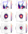 |
Fig. 1. Gaia DR3 CMD of the SMC (top-left) and the LMC (top-right) sources. In the plots, the regions used to select the supergiants (blue) and the RGB stars (red) are marked. The respective final selections (see text for details) of the RGB stars (pink) and supergiants (light blue) of the Clouds are also over-plotted. The middle-left and bottom-left show the number density distribution of the selected RGB and supergiant sources within ∼11 deg of the SMC from its centre (RA = 12.80 deg and Dec = −73.15 deg; Cioni et al. 2000). The middle-right and bottom-right panels show the distribution of the RGB and supergiant sources within ∼20 deg of the LMC from its centre (RA = 81.24 deg and Dec = −69.73 deg; van der Marel & Cioni 2001). The distributions are shown in zenithal equidistant projection coordinates X and Y, as defined in van der Marel & Cioni (2001). For the LMC we show a de-projected spatial distribution (refer to Sect. 2.2). The colour bar from black to yellow represents the increasing stellar densities in all the plots. |
2.2. Gaia DR3–XP spectra for LMC sources
A similar procedure to the one adopted for the SMC in the previous section is followed to select the LMC sources, but using a 20 deg radius from its centre (RA = 81.24 deg and Dec = −69.73 deg; van der Marel & Cioni 2001). Our base LMC sample consists of 27 231 400 objects, which includes stellar populations of different ages as shown on the top-right panel of Figure 1. Since there are many objects in the LMC and our interest lies in the RGB and supergiant stars, we initially applied the selection criteria provided by Gaia Collaboration (2021b) for extracting these two populations from the CMD. To select LMC RGB sources we use as vertexes of the polygon [GBP–GRP, G]: [0.80, 20.5], [0.90, 19.5], [1.60, 19.8], [1.60, 19.0], [1.05, 18.41], [1.30, 16.56], [1.60, 15.3], [2.40, 15.97], [1.95, 17.75], [1.85, 19.0], [2.00, 20.5] and [0.80, 20.5] and to select LMC supergiants we use instead [GBP–GRP, G]: [0.90, 18.25], [0.1, 15.00], [−0.30, 10.0], [2.85, 10.0], [1.30, 16.56], [1.05, 18.41] and [0.90, 18.25]. The panels on the middle- and bottom-right of Figure 1 show the distribution of the selected 520 338 RGB and 99 323 supergiant stars of the LMC, respectively.
The LMC is an inclined disc galaxy, and it is important to de-project the spatial distribution from the sky plane to the galaxy plane. Hence, the inclination (i) of the LMC disc with respect to the sky plane and the position angle of the line of nodes (θ) are taken into account to estimate the de-projected X′ and Y′ coordinates. We applied the recent estimates of i = 23.26 deg and θ = 160.43 deg from Gaia Early DR3 (Saroon & Subramanian 2022) and used the distance estimate of ∼50 kpc from de Grijs et al. (2014). The de-projected spatial distribution is used hereafter for the LMC during the entire analysis.
3. Synthetic Strömgren photometry using Gaia DR3–XP spectra
Bengt Strömgren introduced a narrow-band photometric system with four (u: 350 nm, v: 410 nm, b: 467 nm and y: 547 nm) bandpass filters (refer to Strömgren 1963, 1964 for more details) covering a similar range as the UBV photometric system. These narrow Strömgren bands are intentionally designed to match the specific signatures in the spectra of stars that directly relate to the physical properties Teff, log g and [Fe/H] and therefore allowed us to classify stars of different spectral classes (Strömgren 1964). Subsequent studies (e.g. Grebel & Richtler 1992) built on the photometric system devised by Strömgren, and derived calibration relations to estimate photometric metallicities of RGB stars (Hilker 2000; Calamida et al. 2007; Hughes et al. 2014; Narloch et al. 2021, 2022; Bellazzini et al. 2023 and references therein) and supergiants (Grebel & Richtler 1992; Árnadóttir et al. 2010; Piatti et al. 2019). These studies provided metallicity estimates also for stars in the Clouds and of star clusters.
Gaia Collaboration (2023) and De Angeli et al. (2023) explored the details of Gaia DR3–XP spectra, and also the generation of synthetic photometry in bands that are covered by the Gaia BP/RP wavelength ranges. However, the residual systematics in the externally calibrated XP spectra have larger discrepancies when compared with the existing photometry, notably at λ < 400 nm. Cordoni et al. (2023) also produced synthetic photometry in BVI bands from the Gaia DR3–XP spectra, and validated the accuracy of the synthetic photometric conversion using GaiaXPy by comparing it with literature values. The GaiaXPy is a Python tool from the Data Processing and Analysis Consortium (DPAC) that allows the generation of synthetic photometry in a set of desired systems from the input internally calibrated, continuously represented mean spectra (see Gaia Collaboration 2023 for more details). Gaia Collaboration (2023) used a second-level calibration called standardisation to reproduce existing photometry in several widely used systems to millimag accuracy. Section 4 of Gaia Collaboration (2023) discusses the potential of XP spectra by estimating the synthetic Strömgren magnitudes, as a test case, and deriving photometric metallicities. In our study, we followed a similar method. First, we queried the Gaia archive to obtain the Gaia DR3–XP spectra for a list of probable SMC and LMC sources. Then, we used the GaiaXPy tool to derive the standardised synthetic Strömgren magnitudes (v, b and y). We note that the standardisation was not done for the u band, and the calibration relations we chose do not utilise it. Hence, we did not use it in our analysis. GaiaXPy also provides us with fluxes and flux errors on each of the Strömgren bands.
4. Estimation of photometric [Fe/H]
4.1. Calibration relation for RGB stars
In a recent study Bellazzini et al. (2023) estimated the photometric metallicities of Galactic giant stars by utilising synthetic Strömgren magnitudes from Gaia DR3–XP spectra. Their metallicities derived from the empirical calibration relations provided by Calamida et al. (2007), reported in equation (1), have a typical accuracy of ≤0.1 dex in the range −2.2 < [Fe/H] < −0.4 dex. They also found a systematic trend with [Fe/H] at a higher metallicity, beyond the applicability range of the calibration relation. Metallicities derived using the Hilker (2000) calibration are less precise, and show particularly lower accuracy in the metal-poor regime when compared with the spectroscopic metallicities from APOGEE.
![Mathematical equation: $$ \begin{aligned} \text{[Fe/H]} = \frac{(m_{1,0} - \gamma * (v - y)_0 - \alpha )}{\delta * (v - y)_0 + \beta } , \end{aligned} $$](/articles/aa/full_html/2025/08/aa52510-24/aa52510-24-eq1.gif) (1)
(1)
where α = −0.312, β = −0.096 ± 0.002, γ = 0.513 ± 0.001, δ = 0.154 ± 0.006 and m1 = (v − b)−(b − y).
In this study, we used the Calamida et al. (2007) calibration to calculate the iron abundance [Fe/H] of the SMC and LMC RGB stars. To correct for extinction, we used the reddening maps of the Clouds provided by Skowron et al. (2021), where the extinction is estimated using the red clump giant stars. Their maps cover areas corresponding to a distance from the centre of the galaxies of 2.5 deg for the SMC and 6.5 deg for the LMC. In the outer regions, which are not covered in Skowron et al. (2021) maps, the extinction is corrected by using the all-sky reddening map of the MW provided by Schlegel et al. (1998). The maps provide median E(B − V) values, and for each of the sources in our study, we used the nearest region to obtain their extinction values. The reddening values E(V − I) provided by Skowron et al. (2021) can be converted into E(B − V) by using the recalibration by Schlafly & Finkbeiner (2011). As the recalibration suggests, we translated the E(V − I) into E(B − V) by E(B − V) = (E(V − I)/1.237)×0.86. We obtain the dereddened colour indices, m1, 0 = m1 + 0.24 × E(B − V), (v − y)0 = (v − y)−1.24 × E(B − V), and (b − y)0 = (b − y)−0.74 × E(B − V) using the equation from Crawford & Mandwewala (1976).
The applicability range of equation (1) is 0.85 ≤ (v − y)0 ≤ 3, which reduces our SMC and LMC RGB samples to 78 473 and 512 367 sources, respectively. Then, using equation (1), we estimate the photometric metallicities of the SMC and LMC RGB stars, finding a significant spread. On further investigation, it is clear that this is due to those sources with magnitude uncertainties in each band > 0.1 mag; eliminating them resulted in 57 512 SMC and 214 603 LMC RGB stars. The CMDs in Figure 2 clearly illustrate the range of (v − y)0 colours of our selected RGB stars in the SMC (first plot) and LMC (second plot) using Strömgren bands, which are also over-plotted in the Gaia CMDs (Figure 1). We followed the error propagation to estimate the uncertainties on the metallicities, and the estimated median error of both samples is around 0.6 dex. In Figure 3, the distribution of the estimated metallicities (top-left) and the estimated errors (bottom-left) for both galaxies are provided. The estimation of [Fe/H] involved multiple quantities, all of which were propagated which resulted in large uncertainties. The distribution shows that the majority of the sources have uncertainties < 1 dex, with on average larger values for supergiants than for RGB stars. We did not limit the uncertainties of the metallicities in our study, which is then based on the full sample.
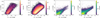 |
Fig. 2. Colour-magnitude diagrams depicting the final selection of RGB stars in the SMC (first plot) and those in LMC (second plot), both use Strömgren bands. The third and fourth plots present the CMDs of the final selection for supergiants in the SMC and in LMC, also using Strömgren bands. |
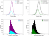 |
Fig. 3. Metallicity distributions of RGB (top-left) and supergiant (top-right) stars of the LMC and SMC samples. Best-fit Gaussians for the SMC (cyan) and the LMC (purple) are shown on the histograms. The distributions of the estimated uncertainties are also shown for RGB stars (bottom-left) and for supergiants (bottom-right). Best-fit Gaussians for the SMC (green) and the LMC (black) are marked. |
4.2. Calibration relation for supergiant stars
To estimate the metallicities of the supergiant stars, we used the empirical relations provided by Grebel & Richtler (1992), and reported in equation (2). They successfully performed a feasibility study to apply this equation to the supergiants in the young stellar cluster NGC 330, and also to some field stars of the SMC around the cluster. Later, a study by Piatti et al. (2019) applied this relation to estimate the metallicities of the supergiant stars in selected young clusters of the Clouds.
![Mathematical equation: $$ \begin{aligned} \text{[Fe/H]} = \frac{(m_{1,0} + a_1 * (b - y)_0 + a_2)}{a_3 * (b - y)_0 + a_4}, \end{aligned} $$](/articles/aa/full_html/2025/08/aa52510-24/aa52510-24-eq2.gif) (2)
(2)
where a1 = −1.240 ± 0.006, a2 = 0.294 ± 0.030, a3 = 0.472 ± 0.040 and a4 = −0.118 ± 0.020.
We followed the same method as explained in Sect. 4.1 to estimate the reddening values. Then, we estimated the extinction values in the visual band AV = 3.1 × E(B − V). We used the translation equation from Cardelli et al. (1989) and we estimated the extinction in each Strömgren band by using Av = 1.397 × AV, Ab = 1.240 × AV and Ay = 1.005 × AV. The applicability range of equation (2) is 0.4 ≤ (b − y)0 ≤ 1.1 and this reduced the SMC sample to 21 207 sources and the LMC sample to 71 628 sources. Using equation (2), we estimated the photometric metallicities of the supergiant sources in both galaxies. Similarly to the RGB stars, we removed sources with magnitude uncertainties in each band > 0.1 mag, which results in 20 713 SMC and 69 083 LMC supergiants. Figure 2 shows the range of (b − y)0 colours for our selected supergiant stars in the SMC (third plot) and LMC (fourth plot) using the Strömgren bands. The distribution of the estimated metallicities of the SMC and LMC supergiants are shown on the top-right panel of Figure 3. We also estimated the uncertainties for our [Fe/H] values using error propagation, and obtained a median error of around 0.8 dex for the SMC and around 0.6 dex for the LMC samples. The propagated error distribution for both galaxies are shown in the bottom-right panel of Figure 3. As for RGB stars, no further reduction has been applied based on the errors.
We chose to utilise the Grebel & Richtler (1992) calibration for supergiants and the Calamida et al. (2007) for our RGB samples for the following reasons. Calamida et al. (2007) offers a new empirical metallicity calibration using (u − y) and (v − y) colours, which are more sensitive to temperature across a broader metallicity range of −2.2 < = [Fe/H] < = −0.7 dex, providing an advantage over Grebel & Richtler (1992). Additionally, Bellazzini et al. (2023) successfully applied the Calamida et al. (2007) calibration for estimating metallicity in Galactic giant stars, yielding accurate results. However, Gaia Collaboration (2023) noted that this calibration, based on older globular clusters, may introduce systematic offsets when applied to younger systems, such as open clusters, due to intrinsic age differences. In contrast, despite its limited sources, the Grebel & Richtler (1992) calibration is applicable to red supergiants, making it more suitable for our purpose of estimating metallicities for these stars.
5. Results
5.1. Metallicity distributions
The histograms in the top-left and top-right panels of Figure 3 depict the metallicity distributions of the RGB stars and supergiants of the Clouds, respectively. We excluded sources with [Fe/H] and uncertainties outside the broad range illustrated in Figure 3, resulted in 271 843 RGB stars and 89 599 supergiants in the Clouds after removing duplicate sources in the outskirts. By comparison, the overall metallicity of the SMC RGB stars is lower than that of the LMC, as expected, which is also the case for the supergiants. For both populations, we obtained unimodal metallicity distributions in agreement with the previous studies (Carrera et al. 2008; Dobbie et al. 2014; Choudhury et al. 2016; Grady et al. 2021; De Bortoli et al. 2022). These literature metallicity distributions also show significant asymmetries, with sharp declines towards the metal-rich ends, and extended tails towards the metal-poor ends (see e.g. Grady et al. 2021). We do not see these trends in our metallicity distributions, probably because of the large errors on the individual metallicity estimates (Figure 3). We recognise that while the shape of our metallicity distributions may have limitations due to larger uncertainties, our focus is on the mean (median) metallicities because our main goal is to produce maps of the mean metallicity and mean metallicity gradients. To further compare the metallicity distributions, we estimated the peak and dispersion values by fitting a Gaussian to each of the histograms. The peak metallicity and the dispersion of the LMC RGB stars is −1.19 ± 0.51 dex, whereas for the supergiants, it is −0.58 ± 0.77 dex. In the SMC, the RGB stars show a peak metallicity and a dispersion of −1.47 ± 0.49 dex while that of the supergiants is of −1.08 ± 0.54 dex. There could also be larger systematic errors in these estimates, for instance, caused by errors in the calibration or between the RGB stars and the supergiants. Grady et al. (2021) estimated the median metallicity of RGB stars within 12 deg of the LMC to be −0.78 dex. Haschke et al. (2012) obtained a mean [Fe/H] of −1.50 ± 0.24 dex based on RR Lyrae stars in the LMC. Previous studies such as Dobbie et al. (2014) and Choudhury et al. (2016) found the median [Fe/H] to be about −1 dex from the analysis of RGB stars in the inner 4–5 deg of the SMC. Carrera et al. (2008) also quotes a similar value of −1 dex for RGB stars in the inner region, but they also note a decrease of the median value towards the outer region of the galaxy. In the SMC, Haschke et al. (2012) obtained −1.70 ± 0.27 dex based on RR Lyrae stars. Our estimates for both the LMC and SMC RGB stars are lower compared to the median values estimated previously. This could be due to the fact that our metallicity distributions include stars in large areas encompassing the SMC and LMC outer regions, which are predominantly populated by metal-poor and old stars. However, a recalibration of our metallicities using the APOGEE data shows a systematic difference of about 0.4 dex (see Sect. 5.2), which would bring our estimates in line with those from previous studies. If we were to limit our sample by applying cuts based on the individual metallicity errors (e.g. 0.3 dex), it would be reduced to only a few thousand sources. Irrespective of our large uncertainties, we see that our median metallicity estimates align with those from previous studies. Hence, we did not apply further cuts in order not to reduce the statistical significance of our analysis. We examined our initial selection of photometric and astrometric cuts to assess how different criteria impact the resulting metallicity distributions. Our findings indicate that the metallicity distributions (Figure 3) remain unchanged when using ruwe ≤1.2, and applying a photometric error of < 0.1 mag instead of < 0.22 mag as adopted in all three Gaia bands.
5.2. Photometric metallicity recalibration
In order to validate the estimates of the photometric metallicities of the RGB and supergiant samples from our work, we compared them with the spectroscopic metallicities from APOGEE. APOGEE is a high-resolution (R∼22 000), near-infrared (H band; 1.51–1.7 μm) spectroscopic sky survey. In the southern sky, observations are performed with the 2.5m du Pont telescope at Las Campanas Observatory, Chile. The initial samples of sources in the LMC and SMC regions were ∼70 000. Though the survey mainly focused on the RGB stars, it also included main sequence stars, asymptotic giant branch (AGB) stars and post-AGB stars. The details on the target selection are explained in Zasowski et al. (2017). The ASPCAP (APOGEE Stellar Parameters and Chemical Abundances Pipeline) calculates the stellar parameters and elemental abundances. We cross-matched the APOGEE sources with the Gaia DR3 data, to select the most probable members of the Clouds and retain those with parallax ≤0.2 mas which eliminates foreground MW sources within ∼5 kpc. Furthermore, we applied the proper motion selections (1 ≤ μα ≤ +2.5 mas yr−1 and −0.8 ≤ μδ ≤ 1.5 mas yr−1) to identify the most probable LMC sources (Saroon & Subramanian 2022). This selection criteria removes many sources, and we are left with a sample of ∼14 135 sources. Along with the cut in the parallax to remove the foreground contamination from the MW, we also discarded the SMC sources whose proper motions lie outside the expected range (−3 ≤ μα, μδ ≤ +3 mas yr−1) as predicted by the simulations (Diaz & Bekki 2012) for the main body and stellar tidal features around the SMC. We recalibrated our photometric estimates to match the zero-points of both our samples (Appendix A). This is done by cross-matching the APOGEE sample of the SMC and LMC RGB sources with our samples after the elimination of sources with large photometric uncertainties. The crossmatched sources (4308) then have both the spectroscopic metallicity estimates from APOGEE [Fe/H]spec and the photometric metallicity estimates from our study [Fe/H]phot. We estimated the peak of [Fe/H]spec and [Fe/H]phot from Gaussian fitting and computed their difference, which is about −0.43 ± 0.02 dex, for both the SMC and the LMC RGB samples. This value is used to obtain the recalibrated metallicities such as [Fe/H]recal = [Fe/H]phot + 0.43 dex. Bellazzini et al. (2023) also used a similar method to recalibrate the metallicity estimates of their MW sources. Following a similar procedure for supergiant stars, we found 1212 crossmatches with APOGEE. The peak difference obtained is −0.35 ± 0.01 dex. Hence, the recalibrated metallicities is obtained as [Fe/H]recal = [Fe/H]phot + 0.35 dex. Bellazzini et al. (2023) found a smaller shift of about 0.14 dex for MW stars. The spatial distribution of the Clouds (see Figure 1) indicates that there is a decreasing completeness towards the centre of the galaxies. This suggests an increased level of crowding that can lead to blending and contamination of XP spectra. This may impact our estimation of the photometric metallicities, especially at the centre of the Clouds (Rathore et al. 2025b). In this context, to better understand the larger shifts obtained in our study, we performed a test to determine whether the peak difference between our photometric metallicities and spectroscopic sample decreases as we move away from the centre of the Clouds (refer to Sect. B and Figures B.1 and B.2).
5.3. Radial recalibration
To maintain consistency in our recalibration with respect to the spectroscopic sample, it is essential to account for variations in the recalibration zero point. This consideration is particularly significant in regions affected by crowding, as they will experience the most impact from radial bias when applying uniform recalibration throughout the galaxy. Our analysis of the two galaxies was conducted separately for the RGB stars. It is evident from the top two rows of Figure B.1 that the peak differences change from the centre to the outskirts. In the bottom-left panel of Figure B.1, we observed that the radial variation of the LMC RGB peak difference is significantly larger at the centre (0.7 dex) than at the outskirts. As we move outward, this difference decreases to 0.3 dex, and then slightly increases to 0.5 dex in the outer regions. However, in the outer bins, the distribution of sources becomes less clear due to the reduced number of stars present. The important factor contributing to these larger shifts could be crowding, causing an increased spectral contamination. Therefore, radial recalibration is applied to the RGB stars in the LMC. For the defined radial bins shown in Figure B.1, we utilised the corresponding peak difference rather than a constant value. In contrast, the third row of Figure B.1 shows that the RGB stars in the SMC did not exhibit significant radial differences and have larger standard deviations. As a result, we opted for a consistent recalibration factor of 0.4 dex across the entire SMC.
We encountered limitations regarding the SMC supergiants due to an insufficient number of cross-matched sources from the APOGEE survey. This indicates that significant differences may not be detectable between our photometric and spectroscopic samples. Therefore, we did not further separate the LMC and SMC supergiants (Figure B.2). The middle plot in the bottom panel of Figure B.2 primarily represents the SMC supergiant stars based on their radial distance. For all supergiant stars, we observed an overall constant difference of 0.4 dex, with a variation of approximately 0.1 dex only in the bin corresponding to the radial range of 3–4 kpc. Given the large standard deviations, we applied a constant recalibration factor of 0.4 dex.
5.4. Metallicity maps of the RGB and supergiant stars
We produced the metallicity maps for the young (supergiants) and the old (RGB stars) stellar populations separately. In order to do that, we combined the RGB sources from both the SMC and the LMC and removed any duplicate sources, as our initial selection of the LMC and SMC areas overlap in their outer regions. Then, we created a two-dimensional Hess distribution (a density plot) colour-coded with the median of the metallicity of each bin, using the recalibrated metallicity estimates, since the median is less prone to the effect of outliers. The left panel of Figure 4 shows the metallicity map of the RGB stars, where each bin corresponds to 0.25 deg2. Although we tend to have fewer sources in the outskirts of the Clouds than in their inner regions, their overall distribution is a large improvement over the stellar density from previous spectroscopic metallicity studies. The central regions of the LMC reveal a metal-rich inner disc and a southern spiral arm. The bar is not obvious, and we note that at its centre, the metallicity is low, but this area is also influenced by a lack of sources in our sample due to crowding. The median value of each bin represents the underlying population accurately only with a sufficient number of stars, especially when individual measurement uncertainties are significant. To address this, we created metallicity maps using Voronoi binning as shown in Figure 5. Here, we adopted equal density binning, ensuring that each bin has 100 sources, based on the median error derived from Markov chain Monte Carlo (MCMC) simulations (refer to Sect. C for more details). In the left panel of Figure 5, we show the metallicity distribution of RGB stars in the Clouds. The LMC’s central region has a higher metallicity (yellow-green shades), while the SMC displays a scattered, lower metallicity distribution (greener to purple regions). The outer regions of both galaxies transition into lower metallicities, consistent with the expectation that older, less metal-enriched stars dominate the outskirts. This spatial variation reflects the galaxies’ evolutionary histories, with stronger star formation and chemical enrichment at the centres. The gradient from higher to lower metallicity corresponds to typical dwarf galaxy evolution models, while small-scale variations signal complex star formation histories. We also created Voronoi binning plots for the median uncertainty in each bin (see Figure C.2).
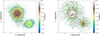 |
Fig. 4. Strömgren photometric metallicity maps of RGB (left) and supergiant (right) stars of the Clouds derived from the Gaia DR3–XP spectra. Each spatial bin corresponds to 0.25 deg2 and 0.5 deg2 for the RGB and supergiant stars, respectively. The maps are centred at RA = 81.24 deg and Dec = −69.73 deg; (van der Marel & Cioni 2001). The bar regions of both galaxies are marked with black ellipses. The colour-coding from blue to white shows the increasing median metallicity values. We note the larger relative difference between the LMC and SMC metallicity in the supergiants than in the RGB stars. The distribution of RGB stars, which contains fainter sources than that of supergiants, at the core of the galaxies may be affected by a lack of sources due to crowding. |
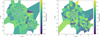 |
Fig. 5. Strömgren photometric metallicity maps of RGB (left) and supergiants (right), respectively. These maps were produced using the Voronoi binning method, where each bin has 100 sources. The colour-coding from green to yellow indicates an increase in the metallicity. |
Recently Frankel et al. (2024) produced a metallicity map of the entire LMC using total metallicity estimates ([M/H]) from Andrae et al. (2023). Their maps confirm an extended disc between −1.6 dex and −0.8 dex compared to a smaller disc at metallicities below −1.6 dex or above −0.8 dex. The bar region dominates at all metallicities, but spiral features are not as prominent as in our map. Grady et al. (2021) provided the metallicity maps of the Clouds using the Gaia DR2 data. Their maps also reveal a metal-rich LMC bar and a metal-rich SMC centre. In the outer regions, the metallicity further decreases, as we see also in our maps. The right panel of Figure 4 provides the metallicity map of the supergiant (young) stars of the Clouds using bins with a size of 0.5 deg2 due to the reduced number of sources. Similarly to the most metal-rich maps by Frankel et al. (2024), we trace the extent of the inner LMC disc superimposed to a wide metal-poor outer region, but we do not find a clear enhancement corresponding to the bar of the galaxy. In the SMC, our map clearly traces a metal-rich bar-like feature at its centre, which is however, metal-poor than at the centre of the LMC. The young populations are metal-rich than the old ones, as previously noticed (Figure 3), and their spatial distribution differs. A similar trend can be seen in the right panel of Figure 5, which shows the Voronoi-based metallicity distribution of supergiants in the Clouds. Each bin has 100 stars, and the colour scale indicates metallicity levels, with yellow representing high metallicity and purple indicating low metallicity. These findings align with previous research, such as Grady et al. (2021), which highlighted the LMC’s inside-out formation and the SMC’s bursty star formation history. Additionally, Frankel et al. (2024) noted the impact of interactions between the LMC and SMC on their metallicity distributions, further explaining the observed differences. Both of these works utilised different machine learning methods, which shows dependency on their respective training samples. For example, in Figure 8 of Frankel et al. (2024), it is evident that the difference in [M/H] estimates between their work, and the APOGEE DR17 sources is less than 0.2 dex for G ≤ 16.5 and less than 0.4 dex at fainter magnitudes, which is closer to the 0.43 dex of constant recalibration as we obtained for the RGB sample in our study. But the figure also includes differences from other spectroscopic surveys, which show a wider range than the APOGEE DR17 data. It is important to note that a large number of sources from APOGEE were used to train the XGBoost algorithm (Andrae et al. 2023) utilised by Frankel et al. (2024). Therefore, the observed smaller differences could be biased due to this training on APOGEE DR17 data. Both of these works demonstrate the ability of data-driven methods to estimate the photometric metallicities for a larger sample of stars, but focused exclusively on the older population. This is understandable, as there is a larger amount of spectroscopic data available for the RGB stars to train such models. In contrast, our work aims to estimate the metallicities of a larger sample of stars that includes both young and old stellar populations using the same method. This approach is particularly beneficial for galaxies such as the Clouds, where studying populations of different ages is essential to understanding their complex interaction history.
5.5. Metallicity gradient of RGB stars
To further explore the metallicity distribution of the SMC and LMC RGB stars, we derived the metallicity gradients separately for the two galaxies as a function of distance from their corresponding centres. In the SMC, we first converted the distance from degrees into kpc by using 62 kpc × tan(radius), where 62 is the distance to the galaxy from de Grijs & Bono (2015). Then, we radially binned the sources into 0.2 kpc steps up to 2 kpc from the centre. We used 0.5 kpc steps up to 6 kpc, 1 kpc steps up to 8 kpc and combined the rest of the sources until 11 kpc into a single sub-region. We chose radial bins of different radii due to the decreasing stellar density from the centre towards the outskirts. The number of sources in each bin ranges from around 550 to a few thousand in the central bins to around 270 in the outer ones. The metallicity gradient of the SMC RGB stars as a function of distance is shown in the bottom-left panel of Figure 6. For this, we calculated the median metallicities in each of the radial bins and also their respective standard errors. We used the Python module curve-fit to find the estimate of the best-fit metallicity gradient. We observed a linearly decreasing trend, and a negative metallicity gradient of −0.048 ± 0.007 dex kpc−1. In the figure, the gradient is superimposed on the distribution of the estimated individual stellar metallicities.
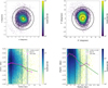 |
Fig. 6. Distribution of RGB stars within the SMC (top-left) and the LMC (top-right) with superimposed annular rings of breakpoints marked in the corresponding lower panels. The plots show the metallicity gradients for the SMC (bottom-left) and LMC RGB stars (bottom-right). The median metallicities of the annular bins are marked with pink stars along with their standard errors. Linear best-fits are marked with green and the piecewise-regression fits are marked with grey. The black vertical lines show the division of different segments or the location of the breaks in the gradient. In both panels, a Hess diagram shows the density distribution of the sources colour-coded such that blue shows the regions with the highest stellar density. |
Although we can estimate the overall gradient by using a linear fit, it is evident from the median values that the slope changes are not uniform across the SMC, but there are breaks in the gradient. To quantify these changes in the slope, we used the Python module piecewise-regression or segmented regression (Pilgrim 2021). This module is particularly useful in estimating the different slopes in the dataset without having to fit different slopes in different regions. This module uses an iterative method to identify breakpoint positions and simultaneously fits a linear regression model to data that includes one or more breakpoints corresponding to the gradient’s changes. This makes it computationally efficient and allows for robust statistical analysis. We iterated the fit over various numbers of breakpoints, starting from zero, which means no breaks in the overall gradient until the model converges. Then we obtain the Bayesian information criterion (BIC), which takes into account the value of the likelihood function to avoid over-fitting and choose the number of breaks where the BIC is minimum as the best-fit model. For the SMC, the best-fit model has three breaks, and we have four regions with different gradient values. All these breakpoints are marked as black concentric circles in Figure 6 (top-left). The different regions and their gradients are provided in Table 1.
Best-fit radial metallicity gradient for the SMC sources.
We followed the same procedure to estimate the metallicity gradient of the LMC RGB stars. One difference is that the LMC metallicity gradient is quoted as a function of the de-projected distance. Then, using 50 kpc × tan(radius), where 50 is the distance to the galaxy from de Grijs et al. (2014), we obtained the de-projected distance in kpc. Also, in comparison with the SMC, our LMC sample is larger, and hence we redefined the size of our radial bins as follows. We radially binned the sources into 0.2 kpc steps up to 7 kpc from the centre. Then, we used 0.5 kpc steps up to 10 kpc, 1 kpc steps up to 13 kpc and combined the rest of the sources until 20 kpc into a single sub-region. The median metallicity of each of these sub-regions is estimated along with their standard errors and shown in Figure 6. The linear best-fit for the overall metallicity gradient is also shown and suggests an increasing metallicity until ∼2.5 kpc from the centre. Although in these regions we can have the highest stellar density, Gaia DR3 is incomplete and sources are still missing. The metallicity gradient corresponds to −0.062 ± 0.005 dex kpc−1. Our best-fit model for the segmented regression returns four breakpoints, and hence five line segments with different gradients are as given in Table 2. The overall metallicity gradient for the entire region is also provided at the bottom of the table. The breakpoints are marked as concentric circles in Figure 6 (top-right). To facilitate the comparison with previous studies, we repeated the analysis by using radial bins in degrees. The resulting metallicity gradients for the SMC and LMC RGB stars are given in the top-left and top-right panels of Figure D.1, respectively, and the values are provided in the appendix.
Best-fit radial metallicity gradient for the LMC sources.
5.6. Metallicity gradient of supergiants stars
We present here the metallicity gradient as a function of the distance (kpc) of the young supergiant stars in both the SMC and the LMC. We used the same radial binning that was applied to the SMC RGB sample. The metallicity gradients of the supergiant stars are shown in Figure 7 (bottom). We also used the same Python curve-fit module to fit the median metallicities of different radial bins and derive the best-fits. In the SMC, we find a linearly decreasing trend in the metallicity distribution, and the estimated metallicity gradient is −0.045 ± 0.007 dex kpc−1. The best-fit for the piecewise-regression method has only one break around 1 kpc corresponding to two gradient values. We redefined our radial binning for the LMC supergiant sources. For the LMC supergiants, we radially bin the sources into 0.2 kpc steps up to 7 kpc from the centre. Then, we use 0.5 kpc steps up to 10 kpc, 1 kpc steps up to 16 kpc and combined the rest of the sources until 20 kpc into a single sub-region. In the LMC, we find a peculiar trend in the median metallicities of the supergiant stars, which can possibly be due to their intrinsically non-uniform spatial distribution. Most of these sources are concentrated in the bar region and in the major spiral arm of the LMC. At about 5 deg from the LMC centre, the stellar density drops rapidly, where the median metallicities tend to decrease abruptly. Towards the outskirts of the LMC, the stellar density distribution is very low but more or less uniform, and hence the median metallicity values seem to flatten. The estimated metallicity gradient from the LMC supergiants is −0.065 ± 0.007 dex kpc−1. The best-fit for the piecewise-regression is obtained with two breaks and three gradients. In the inner region, we have a positive metallicity gradient, and then we have negative gradients with a break around 4 kpc. Beyond 7 kpc, we obtain an almost flat gradient value. The different regions and their metallicity gradients for the SMC and the LMC supergiants are provided in Tables 1 and 2, respectively.
5.7. Metallicity catalogue
The final catalogues for all the sources with estimated [Fe/H], recalibrated using the APOGEE values, are published with this study. As an example, the estimated [Fe/H] values along with the reddening values and other parameters characterising the individual sources (Gaia DR3 Source IDs, coordinates at the epoch J2016.0, Strömgren magnitudes, and distances from the centre of the galaxies) are shown in Table 3.
Catalogue of the estimated [Fe/H] for RGB stars in the SMC.
6. Discussion and conclusions
In this work, we estimated the photometric metallicities from Gaia DR3–XP spectra using the synthetic Strömgren photometry. We used the different calibration relations from the literature to derive the [Fe/H] abundance of the RGB (old, > 3 Gyr old) and the supergiant (young, < 300 Myr old) stars in the SMC and the LMC. We also compared our photometric metallicity estimates with the spectroscopic metallicities from APOGEE to validate our method. We used our photometric metallicities to create metallicity maps with a spatial resolution of 0.25–0.5 deg2 covering a wide area of the Clouds for both stellar populations. We also computed metallicity gradients with respect to the centres within both galaxies. Our choice of the centres should not influence the gradients because the central and smallest bins correspond to a circular diameter of 0.4 kpc (about 0.4 deg), which includes other estimated centres (e.g. Niederhofer et al. 2021, 2022). In the left panel of Figure 8, we show the comparison of the radial metallicity gradients obtained in our study for the SMC.
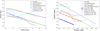 |
Fig. 8. Comparison of the radial metallicity gradients of the SMC (left) and the LMC (right) from this work with those from the literature. |
6.1. SMC gradient
In our study, the estimated overall metallicity gradient of the SMC RGB stars is −0.048 ± 0.007 dex kpc−1, which is very similar to the gradient obtained for the supergiants (−0.045 ± 0.007 dex kpc−1) out to 11 deg (∼10 kpc) from the SMC centre. Povick et al. (2023b) explored the metallicity estimates of the RGB stars from APOGEE and found a similar overall metallicity gradient of −0.0545 ± 0.0043 dex kpc−1 for the SMC stars out to ∼9 kpc. Previously Choudhury et al. (2020) used the RGB slope as an indicator of the average metallicity and estimated a metallicity gradient of −0.031 ± 0.005 dex deg−1 within 2.5 deg of the centre of the galaxy, finding also a rather flat gradient beyond this distance. This is shallower than our current overall estimates but is in good agreement with the gradient we find from RGB stars located within 1–5 deg −0.029 ± 0.003 dex kpc−1. The steeper gradient we find up to 1 kpc from the centre (0.079 ± 0.014 dex kpc−1) might be influenced by the incompleteness of our dataset due to crowding. In the outer regions, the gradient first decreases steeply, the slope is higher than in the innermost regions, and then shows a flattening. A previous study by Parisi et al. (2016) also found, using star clusters, a change of slope at about 5 kpc, suggesting an upturn of the gradient until 8 kpc. In this less gravitationally bound region, the imprints of dynamical interactions are strong and there are existing sub-structures (e.g. El Youssoufi et al. 2021) which may influence the metallicity distribution. The supergiants also show an increase and then a decrease in the metallicity gradient. Our estimated best-fit for the inner region up to 1 kpc is 0.148 ± 0.086 dex kpc−1 and beyond that it is −0.058 ± 0.008 dex kpc−1. The only breakpoint we find in the centre could again be the result of crowding and not an actual breakpoint in the metallicity gradient.
The spectroscopic study by Dobbie et al. (2014) estimated an RGB metallicity gradient of −0.075 ± 0.011 dex deg−1 out to 5 deg from the centre. Later, Taibi et al. (2022) derived the radial metallicity gradients of several Local Group galaxies, recalibrating the metallicity estimates from Dobbie et al. (2014). Although they have not provided metallicity gradients for different regions across the SMC, their smoothed SMC radial metallicity profile excellently matches the metallicity gradient of SMC RGB stars in our study. Interestingly, they also see a positive gradient up until 1 kpc from the SMC centre, which was not clearly seen or noted in other studies. Then, their gradient decreases until 4 kpc, slightly increases until 5 kpc and then decreases further until 7 kpc in line with the trends found in this study. We note that a change of slope at ∼4 kpc could be deduced from Figure 6, but it is not sufficiently strong to be picked up in our analysis as a separate breakpoint. De Bortoli et al. (2022) estimated a negative gradient of −0.08 ± 0.03 dex deg−1 in the inner region (< 3.4 deg), but a positive or null gradient in the outer region 0.05 ± 0.02 dex deg−1 derived from the analysis of SMC field stars. Their values are comparable to the main-body cluster metallicity gradients derived in the same study. However, they do not find any separate metallicity gradient for their metal-rich and metal-poor clusters.
Although our estimated overall metallicity gradient seems to overlap with previous studies, it can still be seen that the gradient in different regions differs considerably. One reason could be how we are projecting the SMC stars and estimating the gradients, as the SMC has a large line-of-sight depth and a complex structure. Taking this into account, Dias et al. (2022) showed that any projected radial metallicity gradient cannot be seen when using the real three-dimensional (3D) physical distances to the clusters. Our dataset does not consist of any standard candles to estimate distances based on them. Also, at the distance of the Clouds, estimating the 3D distances for individual stars is not trivial.
6.2. LMC gradient
For the RGB stars across the entire LMC, we obtained an overall metallicity gradient of −0.062 ± 0.005 dex kpc−1, whereas for supergiants we obtained a negative gradient of −0.065 ± 0.007 dex kpc−1. In the right panel of Figure 8, we show the comparison of the radial metallicity gradients obtained in our study for the LMC. A recent study by Povick et al. (2023a) estimated a metallicity gradient of the LMC to be −0.02966 ± 0.00171 dex kpc−1 out to a radial distance of ∼10 deg using spectra of RGB stars from APOGEE, which is shallower than our estimations. They also detect a steepening of the abundance gradients in the inner region of the galaxy for populations younger than 2 Gyr. Grady et al. (2021) utilised the Gaia DR2 data and estimated metallicities using a machine learning method to obtain −0.048 ± 0.001 dex kpc−1 out to ∼12 deg. Also, a previous estimate from Cioni (2009) using the AGB stars in the LMC found a linearly decreasing gradient of −0.047 ± 0.003 dex kpc−1 out to ∼8 kpc from the centre. A study by Choudhury et al. (2016) estimated photometric metallicities and found a similar [Fe/H] trend in the LMC as −0.049 ± 0.002 dex kpc−1 out to ∼4 kpc. In a later study using the VMC data of the RGB stars, Choudhury et al. (2021) estimated a metallicity gradient of −0.008 ± 0.001 dex kpc−1 out to a radius of ∼6 kpc from the LMC centre. This value compares well with our measurement in 2–5 kpc, whereas the overall gradient is somewhat lower compared to the previous studies, probably because our study extends to 20 deg and includes the outskirts of the galaxy, where there is a relatively large number of metal-poor stars.
Our best-fit for the piecewise-regression fit estimates of the metallicity of RGB stars results in four different gradients for the entire LMC. In the very centre until 2 kpc, we get a positive gradient of 0.127 ± 0.026 dex kpc−1. This is the region that mostly encompasses the bar, which has both young and old stars. Also, this is the region that is subject to crowding. In a way, the first breakpoint in the gradient more or less separates the bar from the rest of the galaxy. From 2 to 5 kpc, representing the inner disc of the LMC, we find a gradient of −0.050 ± 0.008 dex kpc−1. A recent study by Rathore et al. (2025b) finds that the angular momentum section of the inner disc is misaligned with respect to the outer disc, which can be reproduced in simulation by a recent collision with the SMC. In our study, a break in the metallicity gradient at 5 kpc corresponds to a transition in the amount of misalignment, which suggests a possible link between the two behaviours. The misaligned inner disc, influenced by the SMC interaction, may have played a role in the chemical enrichment processes, leading to the differing metallicity profiles. In the regions from 5 to 9 kpc, we find a very steep decrease in the gradient corresponding to −0.169 ± 0.011 dex kpc−1 and in the outskirts beyond 9 until 13 kpc, we obtained a positive gradient of 0.044 ± 0.016 dex kpc−1. This outer disc region hosts different tidal sub-structures and has been mostly influenced by the interactions from the MW and also the SMC, its closest companion. Beyond 13 kpc, we again see a negative gradient of −0.074 ± 0.027 dex kpc−1.
Our best-fit piecewise-regression fit for the supergiants provides two breaks in the metallicity gradient, and the supergiants look more complex than the RGB stars. In the inner region up to 4 kpc, we obtained a positive gradient of 0.025 ± 0.014 dex kpc−1. Similarly to the RGB stars, we can see that the bar region is enclosed within the first breakpoint. For the region between 4 to 7 kpc, we see a much steeper gradient of −0.325 ± 0.036 dex kpc−1. This region includes part of the prominent northern spiral arm, where young stars are forming. Moreover, it exhibits a significant decline in stellar density, which leads to the steep gradient observed here. Additionally, the breakpoint around 4 kpc also suggests a link with the misalignment of the angular momentum (Rathore et al. 2025a), which implies a connection between the LMC’s dynamical response to the collision and its chemical evolution. Beyond 7 kpc, we do not have many stars, but the gradient seems to flatten into 0.003 ± 0.006 dex kpc−1.
Feast et al. (2010) derived the metallicity gradient out to 6 kpc from the LMC centre using two different period-metallicity relations for RR Lyrae stars. They estimated a linearly decreasing gradient of −0.0104 ± 0.0021 dex kpc−1 and −0.0145 ± 0.0029 dex kpc−1, whereas Haschke et al. (2012) obtained a gradient of −0.03 ± 0.07 dex kpc−1 using RR Lyrae stars up to 14 kpc from the LMC centre. They also estimated the gradient only in the innermost 8 kpc and obtained a shallower value of −0.010 ± 0.014 dex kpc−1. Wagner-Kaiser & Sarajedini (2013) derived instead a gradient of −0.0270 ± 0.02 dex kpc−1. In the inner 2–5 kpc we also find a shallower gradient, from the RGB stars, compared to the measurements by Feast et al. (2010) and Haschke et al. (2012). By including regions further away, we also find a decreasing trend for the overall distribution of stars. We note that the RR Lyrae stars are at least 10 Gyr old and represent a stellar population that is on average older than our RGB stars.
6.3. Concluding remarks
The main goal of our study is to validate the potential usage of Gaia DR3–XP spectra to estimate the individual [Fe/H] values across a wide area encompassing the Clouds. This method can be applied to sources fainter than 17.65 mag from the next Gaia data releases to study even larger samples and confirm or refine our findings. The metallicity gradients estimated in this work and in comparison with the literature values show that different tracers do not show the same trends. Compared to previous studies, different trends are also present for tracers that cover different spatial regions. The metallicity gradient results from the combination of different physical processes: the chemical enrichment from stellar evolution, the accretion of gas or stars and the process of radial migration, as well as dynamical interaction displacing stars within galaxies. The present-day LMC and SMC have a complex structure, and to quantify which process dominates at a given distance and for a given stellar population, we need to also study azimuthal variations, which we plan to address in our next study focused on sub-structures.
In the near future, the [Fe/H] as well as the abundance of other chemical elements for a large number of stars making up the range of stellar populations present in the Clouds will be obtained with the new multi-object spectroscopic facilities 4MOST (de Jong et al. 2019) and MOONS (Gonzalez et al. 2020). In particular, 4MOST will target about 200 000 RGB stars and 60 000 supergiants across ∼1000 deg2 from the One Thousand and One Magellanic Clouds fields survey (Cioni et al. 2019), whereas MOONS will focus on RGB stars at specific locations during guaranteed-time observations. These spectra, combined with photometric investigations, will provide an unprecedented view of the system, increasing not only the size of the statistical spectroscopic samples but also the number of diagnostics to study its origin and evolution. Yuxi et al. (2023) has shown the possibility of inferring birth radii for individual stars using cosmological simulations in galaxies such as the LMC. They obtain ∼25% median uncertainties for individual stars if accurate metallicities and ages are available, further supporting a promising application of our results. Our findings highlight the complexity of metallicity gradients and their dependence on different stellar tracers, spatial coverage, and physical processes shaping the evolution of the Clouds.
Data availability
The catalogues are available at the CDS via https://cdsarc.cds.unistra.fr/viz-bin/cat/J/A+A/700/A74
Acknowledgments
We thank the referee for their constructive and insightful comments on our paper. AOO acknowledges support from the Indian Institute of Astrophysics during her visit. SS acknowledges support from the Science and Engineering Research Board of India through a Ramanujan Fellowship and support from the Alexander von Humboldt Foundation. AOO is grateful to the European Space Agency (ESA) for support via the Archival Research Visitor Programme during her stay at ESTEC. BD acknowledges support by ANID-FONDECYT iniciación grant No. 11221366 and from the ANID Basal project FB210003. This work has made use of data from the ESA mission Gaia (https://www.cosmos.esa.int/gaia), processed by the Gaia Data Processing and Analysis Consortium (DPAC, https://www.cosmos.esa.int/web/gaia/dpac/consortium). Funding for the DPAC has been provided by national institutions, in particular, the institutions participating in the Gaia Multilateral Agreement.
References
- Agertz, O., Teyssier, R., & Moore, B. 2011, MNRAS, 410, 1391 [Google Scholar]
- Almeida, A., Majewski, S. R., Nidever, D. L., et al. 2024, MNRAS, 529, 3858 [Google Scholar]
- Andrae, R., Rix, H.-W., & Chandra, V. 2023, ApJS, 267, 8 [NASA ADS] [CrossRef] [Google Scholar]
- Árnadóttir, A. S., Feltzing, S., & Lundström, I. 2010, A&A, 521, A40 [NASA ADS] [CrossRef] [EDP Sciences] [Google Scholar]
- Bagheri, G., Cioni, M. R. L., & Napiwotzki, R. 2013, A&A, 551, A78 [NASA ADS] [CrossRef] [EDP Sciences] [Google Scholar]
- Bekki, K. 2009, MNRAS, 393, L60 [NASA ADS] [CrossRef] [Google Scholar]
- Bellazzini, M., Massari, D., De Angeli, F., et al. 2023, A&A, 674, A194 [NASA ADS] [CrossRef] [EDP Sciences] [Google Scholar]
- Belokurov, V., Erkal, D., Deason, A. J., et al. 2017, MNRAS, 466, 4711 [Google Scholar]
- Calamida, A., Bono, G., Stetson, P. B., et al. 2007, ApJ, 670, 400 [Google Scholar]
- Cardelli, J. A., Clayton, G. C., & Mathis, J. S. 1989, ApJ, 345, 245 [Google Scholar]
- Carrera, R., Gallart, C., Aparicio, A., et al. 2008, AJ, 136, 1039 [Google Scholar]
- Carrera, R., Conn, B. C., Noël, N. E. D., Read, J. I., & López Sánchez, Á. R. 2017, MNRAS, 471, 4571 [Google Scholar]
- Chandra, V., Naidu, R. P., Conroy, C., et al. 2023, ApJ, 956, 110 [CrossRef] [Google Scholar]
- Choi, Y., Nidever, D. L., Olsen, K., et al. 2018, ApJ, 866, 90 [Google Scholar]
- Choudhury, S., Subramaniam, A., & Cole, A. A. 2016, MNRAS, 455, 1855 [NASA ADS] [CrossRef] [Google Scholar]
- Choudhury, S., Subramaniam, A., Cole, A. A., & Sohn, Y. J. 2018, MNRAS, 475, 4279 [NASA ADS] [CrossRef] [Google Scholar]
- Choudhury, S., de Grijs, R., Rubele, S., et al. 2020, MNRAS, 497, 3746 [NASA ADS] [CrossRef] [Google Scholar]
- Choudhury, S., de Grijs, R., Bekki, K., et al. 2021, MNRAS, 507, 4752 [CrossRef] [Google Scholar]
- Cioni, M. R. L. 2009, A&A, 506, 1137 [NASA ADS] [CrossRef] [EDP Sciences] [Google Scholar]
- Cioni, M. R. L., Habing, H. J., & Israel, F. P. 2000, A&A, 358, L9 [NASA ADS] [Google Scholar]
- Cioni, M. R. L., Storm, J., Bell, C. P. M., et al. 2019, The Messenger, 175, 54 [NASA ADS] [Google Scholar]
- Cordoni, G., Marino, A. F., Milone, A. P., et al. 2023, A&A, 678, A155 [NASA ADS] [CrossRef] [EDP Sciences] [Google Scholar]
- Crawford, D. L., & Mandwewala, N. 1976, PASP, 88, 917 [CrossRef] [Google Scholar]
- De Angeli, F., Weiler, M., Montegriffo, P., et al. 2023, A&A, 674, A2 [NASA ADS] [CrossRef] [EDP Sciences] [Google Scholar]
- De Bortoli, B. J., Parisi, M. C., Bassino, L. P., et al. 2022, A&A, 664, A168 [NASA ADS] [CrossRef] [EDP Sciences] [Google Scholar]
- de Grijs, R., & Bono, G. 2015, AJ, 149, 179 [Google Scholar]
- de Grijs, R., Wicker, J. E., & Bono, G. 2014, AJ, 147, 122 [Google Scholar]
- de Jong, R. S., Agertz, O., Berbel, A. A., et al. 2019, The Messenger, 175, 3 [NASA ADS] [Google Scholar]
- Dias, B., Parisi, M. C., Angelo, M., et al. 2022, MNRAS, 512, 4334 [NASA ADS] [CrossRef] [Google Scholar]
- Diaz, J. D., & Bekki, K. 2012, ApJ, 750, 36 [Google Scholar]
- Dobbie, P. D., Cole, A. A., Subramaniam, A., & Keller, S. 2014, MNRAS, 442, 1680 [NASA ADS] [CrossRef] [Google Scholar]
- El Youssoufi, D., Cioni, M.-R. L., Bell, C. P. M., et al. 2019, MNRAS, 490, 1076 [NASA ADS] [CrossRef] [Google Scholar]
- El Youssoufi, D., Cioni, M. R. L., Bell, C. P. M., et al. 2021, MNRAS, 505, 2020 [NASA ADS] [CrossRef] [Google Scholar]
- Fall, S. M., & Efstathiou, G. 1980, MNRAS, 193, 189 [NASA ADS] [CrossRef] [Google Scholar]
- Feast, M. W., Abedigamba, O. P., & Whitelock, P. A. 2010, MNRAS, 408, L76 [NASA ADS] [Google Scholar]
- Frankel, N., Andrae, R., Rix, H. W., Povick, J., & Chandra, V. 2024, arXiv e-prints [arXiv:2403.08516] [Google Scholar]
- Gaia Collaboration (Brown, A. G. A., et al.) 2016, A&A, 595, A2 [NASA ADS] [CrossRef] [EDP Sciences] [Google Scholar]
- Gaia Collaboration (Brown, A. G. A., et al.) 2021a, A&A, 649, A1 [NASA ADS] [CrossRef] [EDP Sciences] [Google Scholar]
- Gaia Collaboration (Luri, X., et al.) 2021b, A&A, 649, A7 [EDP Sciences] [Google Scholar]
- Gaia Collaboration (Montegriffo, P., et al.) 2023, A&A, 674, A33 [CrossRef] [EDP Sciences] [Google Scholar]
- Gonzalez, O. A., Mucciarelli, A., Origlia, L., et al. 2020, The Messenger, 180, 18 [NASA ADS] [Google Scholar]
- Grady, J., Belokurov, V., & Evans, N. W. 2021, ApJ, 909, 150 [Google Scholar]
- Grebel, E. K., & Richtler, T. 1992, A&A, 253, 359 [NASA ADS] [Google Scholar]
- Haschke, R., Grebel, E. K., Duffau, S., & Jin, S. 2012, AJ, 143, 48 [NASA ADS] [CrossRef] [Google Scholar]
- Hilker, M. 2000, A&A, 355, 994 [NASA ADS] [Google Scholar]
- Hughes, J., Wallerstein, G., Dotter, A., & Geisler, D. 2014, MNRAS, 439, 788 [Google Scholar]
- Jacyszyn-Dobrzeniecka, A. M., Skowron, D. M., Mróz, P., et al. 2016, Acta Astron., 66, 149 [NASA ADS] [Google Scholar]
- Jacyszyn-Dobrzeniecka, A. M., Skowron, D. M., Mróz, P., et al. 2017, Acta Astron., 67, 1 [NASA ADS] [Google Scholar]
- Jacyszyn-Dobrzeniecka, A. M., Mróz, P., Kruszyńska, K., et al. 2020, ApJ, 889, 26 [Google Scholar]
- James, D., Subramanian, S., Omkumar, A. O., et al. 2021, MNRAS, 508, 5854 [NASA ADS] [CrossRef] [Google Scholar]
- Li, Y., Jiang, B., & Ren, Y. 2024, AJ, 167, 123 [Google Scholar]
- Mackey, A. D., Koposov, S. E., Erkal, D., et al. 2016, MNRAS, 459, 239 [Google Scholar]
- Mackey, D., Koposov, S., Da Costa, G., et al. 2018, ApJ, 858, L21 [Google Scholar]
- Massana, P., Noël, N. E. D., Nidever, D. L., et al. 2020, MNRAS, 498, 1034 [Google Scholar]
- Massana, P., Nidever, D. L., & Olsen, K. 2023, MNRAS, 527, 8706 [Google Scholar]
- Muraveva, T., Subramanian, S., Clementini, G., et al. 2017, MNRAS, 473, 3131 [Google Scholar]
- Narloch, W., Pietrzyński, G., Gieren, W., et al. 2021, A&A, 647, A135 [NASA ADS] [CrossRef] [EDP Sciences] [Google Scholar]
- Narloch, W., Pietrzyński, G., Gieren, W., et al. 2022, A&A, 666, A80 [NASA ADS] [CrossRef] [EDP Sciences] [Google Scholar]
- Nidever, D. L., Majewski, S. R., Muñoz, R. R., et al. 2011, ApJ, 733, L10 [Google Scholar]
- Niederhofer, F., Cioni, M.-R. L., Rubele, S., et al. 2021, MNRAS, 502, 2859 [Google Scholar]
- Niederhofer, F., Cioni, M.-R. L., Schmidt, T., et al. 2022, MNRAS, 512, 5423 [NASA ADS] [CrossRef] [Google Scholar]
- Noël, N. E. D., Conn, B. C., Carrera, R., et al. 2013, ApJ, 768, 109 [Google Scholar]
- Noël, N. E. D., Conn, B. C., Read, J. I., et al. 2015, MNRAS, 452, 4222 [CrossRef] [Google Scholar]
- Oliveira, R. A. P., Maia, F. F. S., Barbuy, B., et al. 2023, MNRAS, 524, 2244 [NASA ADS] [CrossRef] [Google Scholar]
- Olsen, K. A. G., & Salyk, C. 2002, AJ, 124, 2045 [NASA ADS] [CrossRef] [Google Scholar]
- Omkumar, A. O., Subramanian, S., Niederhofer, F., et al. 2021, MNRAS, 500, 2757 [Google Scholar]
- Parisi, M. C., Geisler, D., Carraro, G., et al. 2016, AJ, 152, 58 [NASA ADS] [Google Scholar]
- Piatti, A. E., Pietrzyński, G., Narloch, W., Górski, M., & Graczyk, D. 2019, MNRAS, 483, 4766 [NASA ADS] [CrossRef] [Google Scholar]
- Pilgrim, C. 2021, J. Open Source Software, 6, 3859 [NASA ADS] [CrossRef] [Google Scholar]
- Povick, J. T., Nidever, D. L., Majewski, S. R., et al. 2023a, arXiv e-prints [arXiv:2309.12503] [Google Scholar]
- Povick, J. T., Nidever, D. L., Massana, P., et al. 2023b, arXiv e-prints [arXiv:2310.14299] [Google Scholar]
- Putman, M., Gibson, B., Staveley-Smith, L., et al. 1998, Nature, 394, 752 [Google Scholar]
- Putman, M. E., Staveley-Smith, L., Freeman, K. C., Gibson, B. K., & Barnes, D. G. 2003, ApJ, 586, 170 [NASA ADS] [CrossRef] [Google Scholar]
- Rathore, H., Besla, G., Daniel, K. J., & Beraldo E Silva, L. 2025a, arXiv e-prints [arXiv:2504.16163] [Google Scholar]
- Rathore, H., Choi, Y., Olsen, K. A. G., & Besla, G. 2025b, ApJ, 978, 55 [Google Scholar]
- Recio-Blanco, A., de Laverny, P., Palicio, P. A., et al. 2023, A&A, 674, A29 [NASA ADS] [CrossRef] [EDP Sciences] [Google Scholar]
- Riello, M., De Angeli, F., Evans, D. W., et al. 2021, A&A, 649, A3 [NASA ADS] [CrossRef] [EDP Sciences] [Google Scholar]
- Ripepi, V., Cioni, M.-R. L., Moretti, M. I., et al. 2017, MNRAS, 472, 808 [Google Scholar]
- Rubele, S., Pastorelli, G., Girardi, L., et al. 2018, MNRAS, 478, 5017 [NASA ADS] [CrossRef] [Google Scholar]
- Saroon, S., & Subramanian, S. 2022, A&A, 666, A103 [NASA ADS] [CrossRef] [EDP Sciences] [Google Scholar]
- Schlafly, E. F., & Finkbeiner, D. P. 2011, ApJ, 737, 103 [Google Scholar]
- Schlegel, D. J., Finkbeiner, D. P., & Davis, M. 1998, ApJ, 500, 525 [Google Scholar]
- Scowcroft, V., Freedman, W. L., Madore, B. F., et al. 2016, ApJ, 816, 49 [NASA ADS] [CrossRef] [Google Scholar]
- Skowron, D. M., Jacyszyn, A. M., Udalski, A., et al. 2014, ApJ, 795, 108 [Google Scholar]
- Skowron, D. M., Skowron, J., Udalski, A., et al. 2021, ApJS, 252, 23 [Google Scholar]
- Strömgren, B. 1963, QJRAS, 4, 8 [NASA ADS] [Google Scholar]
- Strömgren, B. 1964, Rev. Mod. Phys., 36, 532 [Google Scholar]
- Subramaniam, A., & Subramanian, S. 2009, ApJ, 703, L37 [Google Scholar]
- Taibi, S., Battaglia, G., Leaman, R., et al. 2022, A&A, 665, A92 [NASA ADS] [CrossRef] [EDP Sciences] [Google Scholar]
- van den Bosch, F. C. 2002, MNRAS, 331, 98 [CrossRef] [Google Scholar]
- van der Marel, R. P., & Cioni, M.-R. L. 2001, AJ, 122, 1807 [Google Scholar]
- Viswanathan, A., Byström, A., Starkenburg, E., et al. 2024, A&A, submitted [arXiv:2408.17250] [Google Scholar]
- Wagner-Kaiser, R., & Sarajedini, A. 2013, MNRAS, 431, 1565 [NASA ADS] [CrossRef] [Google Scholar]
- Wagner-Kaiser, R., & Sarajedini, A. 2017, MNRAS, 466, 4138 [Google Scholar]
- Yuxi, Lu, Buck, T., et al. 2023, arXiv e-prints [arXiv:2312.07219] [Google Scholar]
- Zasowski, G., Cohen, R. E., Chojnowski, S. D., et al. 2017, AJ, 154, 198 [Google Scholar]
Appendix A: Metallicity recalibration using APOGEE
Figure A.1 shows the metallicity distribution of the RGB sources in common between our sample and APOGEE. We fitted Gaussians to both histograms and estimated the peak and dispersion of each sample. The photometric metallicity peaks at –1.32±0.01 dex and the spectroscopic metallicity peaks at –0.90±0.02 dex; hence the peak difference is 0.43±0.02 dex. We added this difference to our estimated photometric metallicities. The bottom panel shows that after applying a shift, both samples match. We also provided the metallicity distribution plots for the supergiant sources in the top panel of Figure A.2. The photometric and spectroscopic peaks of the supergiants are –0.79±0.01 dex and –0.435±0.002 dex. The bottom panel shows that after adding 0.35±0.01 dex to the photometric metallicity, both samples match.
To provide a quantitative idea of the residual bias and dispersion with respect to spectroscopic measures, the top panel of Figure A.3 shows the density histograms of photometric metallicities vs spectroscopic metallicities of RGB stars in the Clouds. In the bottom panel, we plotted the difference in the photometric and spectroscopic samples over the recalibrated metallicities. We fitted a line and the estimated slope is 0.45 with a constant of –0.33. We tested using these values to recalibrate our metallicities rather than just adding the peak difference estimates. Our overall gradients for the RGB sources of both Clouds did not change even by employing this recalibration, but we noticed larger uncertainties, which would then propagate into the analysis of the gradient. The top panel of Figure A.4 shows the photometric metallicities vs spectroscopic metallicities of the supergiants in the Clouds. In the bottom panel, the difference is plotted against the recalibrated values. Here, we do not see a clear slope for the RGB stars. The estimated slope for the supergiants is 0.13 with a constant value of –0.41. With this calibration, uncertainties for the supergiants would be ever larger.
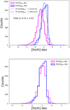 |
Fig. A.1. Histograms of the LMC and SMC sources used for recalibration. On the top panel, the estimated photometric (Phot; blue) metallicities are plotted together with the spectroscopic (Spec; pink) metallicities as measured. On the bottom panel photometric metallicities are exploited after the addition of systematic difference. |
Appendix B: Estimation of peak difference based on radius
Crowding can cause blending and contamination of XP spectra, affecting our estimation of photometric metallicities, especially at the centre of the Clouds. To investigate whether we are observing any amplitude shift from the centre to the outskirts of the Clouds, we divided the area into various annular sub-regions from the respective centres. We plotted the distribution of photometric and spectroscopic metallicities for the LMC RGB stars in the top two rows of Figure B.1, and for the SMC RGB stars in the third row. The radial variation of the shifts from the respective centres are shown in the bottom-left for the LMC RGB stars and bottom-right for the SMC RGB stars. The same analysis was conducted for the supergiant stars and shown in Figure B.2. For both distributions, we fitted Gaussians to identify the peak and standard deviation values for each radial region.
Appendix C: Voronoi binning
In this section, we outline the methodology used to determine an optimal number of sources for plotting the Voronoi metallicity maps of RGB stars and supergiants. To determine a sensible number of sources in each bin, we utilised MCMC simulations. The procedure was as follows: we drew random samples ranging from 10 to 1000, in steps of 10, from our entire dataset and conducted 100 simulations for each sample to determine the median error of [Fe/H]. The results produced a Gaussian distribution, which we fitted to estimate the peak and the associated dispersion, which is our median error for each run. The number of sources is plotted against this error for RGB stars and supergiants (see Figure C.1). Our analysis revealed that for both RGB stars and supergiants, the error of the sample approached ∼0.1 dex when each bin included 100 sources. Consequently, we created a Voronoi metallicity map, ensuring that each of our bins contained 100 sources. Given the significant differences between our LMC and SMC samples, we generated the Voronoi metallicity maps separately for improved visualisation. To facilitate easier interpretation of uncertainties associated with each bin of our Voronoi metallicity maps, we also produced a similar Voronoi binning map where we show the median of the [Fe/H] error in each of the bins. In Figure C.2, the top (RGB stars) and bottom (supergiants) panels show the median error of our metallicity distributions of the LMC (left) and the SMC (right).
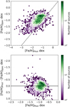 |
Fig. C.2. Photometric [Fe/H] versus spectroscopic [Fe/H] of the RGB sources are shown on the top panel. The dotted line marks the one-to-one relation. In the bottom panel, photometric [Fe/H] (recalibrated with the slope and constant) is plotted against the difference between them. The colour bar from violet to green shows the increase in stellar density. |
Appendix D: Radial [Fe/H] gradient of the SMC and LMC sources in degrees
The overall metallicity gradient as a function of distance (in degrees) is shown in Figure D.1. For both populations in the SMC, we first radially binned the sources into 0.2 deg steps up to 2 deg from the centre. Then we used 0.5 deg steps up to 6 deg, 1 deg steps up to 8 deg and combined the rest of the sources until 11 deg into a single sub-region. The estimated overall metallicity gradient for the SMC RGB stars is –0.053±0.007 dex deg−1, and the overall metallicity gradient estimated for the SMC supergiants is very similar –0.047±0.008 dex deg−1. For the LMC RGB stars and supergiants, we divided the sources into radial bins of 0.2 deg up to 7 deg from the centre and then use 0.5 deg bins up to 10 deg. Due to the lower number density, we made some adjustments for the RGB stars and supergiants. For the RGB stars, we used 1 deg bins up to 13 deg, while for the supergiants, we used 1 deg bins up to 16 deg. Finally, we combined the remaining sources into a single sub-region up to 20 deg. The estimated overall metallicity gradient for the LMC RGB stars is –0.055±0.005 dex deg−1. The overall metallicity gradient estimated for the LMC supergiants is –0.066±0.006 dex deg−1.
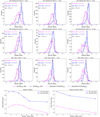 |
Fig. D.1. Radial variation of Photometric versus Spectroscopic metallicities in RGB Stars of the Clouds. The top and middle rows display the peak differences between the photometric (Phot; blue) and spectroscopic (Spec; pink) RGB samples, calculated for various radial ranges from the centre of the LMC. The third row presents similar data for the RGB stars in the SMC. Both peaks are fitted, and the peak values are shown in the last row: on the left for the LMC and on the right for the SMC, which illustrates the radial variation of the shifts from the respective centres. |
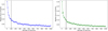 |
Fig. D.3. Median error of [Fe/H] plotted against the number of sources in each bin for RGB (left) and supergiant (right) stars in the Clouds. Dotted vertical lines at 100 sources indicate the limit adopted in our study. |
 |
Fig. D.4. Maps showing the median error in the metallicity of RGB stars (left) and supergiants (right) of the Clouds. These maps are produced using the Voronoi binning method, where each bin has 100 sources. The colour-coding from purple to yellow indicates an increase in the median error. |
 |
Fig. D.5. Radial metallicity gradient (in degrees) for the RGB (top) and supergiant (bottom) stars for SMC (left) and LMC (right). In all panels, the increasing stellar density is colour-coded from purple to yellow. The median metallicities of the annular regions are marked with pink stars along with their standard errors. Linear best-fits and segmented best-fits are shown in green and grey, respectively. The black vertical lines show the division of different segments at the location of the breaks in the gradients. Underlying Hess diagrams show the source-density distributions. |
Best-fit metallicity gradient of the SMC sources in degrees.
Best-fit metallicity gradient of the LMC sources in degrees.
All Tables
All Figures
|
Fig. 1. Gaia DR3 CMD of the SMC (top-left) and the LMC (top-right) sources. In the plots, the regions used to select the supergiants (blue) and the RGB stars (red) are marked. The respective final selections (see text for details) of the RGB stars (pink) and supergiants (light blue) of the Clouds are also over-plotted. The middle-left and bottom-left show the number density distribution of the selected RGB and supergiant sources within ∼11 deg of the SMC from its centre (RA = 12.80 deg and Dec = −73.15 deg; Cioni et al. 2000). The middle-right and bottom-right panels show the distribution of the RGB and supergiant sources within ∼20 deg of the LMC from its centre (RA = 81.24 deg and Dec = −69.73 deg; van der Marel & Cioni 2001). The distributions are shown in zenithal equidistant projection coordinates X and Y, as defined in van der Marel & Cioni (2001). For the LMC we show a de-projected spatial distribution (refer to Sect. 2.2). The colour bar from black to yellow represents the increasing stellar densities in all the plots. |
| In the text | |
|
Fig. 2. Colour-magnitude diagrams depicting the final selection of RGB stars in the SMC (first plot) and those in LMC (second plot), both use Strömgren bands. The third and fourth plots present the CMDs of the final selection for supergiants in the SMC and in LMC, also using Strömgren bands. |
| In the text | |
|
Fig. 3. Metallicity distributions of RGB (top-left) and supergiant (top-right) stars of the LMC and SMC samples. Best-fit Gaussians for the SMC (cyan) and the LMC (purple) are shown on the histograms. The distributions of the estimated uncertainties are also shown for RGB stars (bottom-left) and for supergiants (bottom-right). Best-fit Gaussians for the SMC (green) and the LMC (black) are marked. |
| In the text | |
|
Fig. 4. Strömgren photometric metallicity maps of RGB (left) and supergiant (right) stars of the Clouds derived from the Gaia DR3–XP spectra. Each spatial bin corresponds to 0.25 deg2 and 0.5 deg2 for the RGB and supergiant stars, respectively. The maps are centred at RA = 81.24 deg and Dec = −69.73 deg; (van der Marel & Cioni 2001). The bar regions of both galaxies are marked with black ellipses. The colour-coding from blue to white shows the increasing median metallicity values. We note the larger relative difference between the LMC and SMC metallicity in the supergiants than in the RGB stars. The distribution of RGB stars, which contains fainter sources than that of supergiants, at the core of the galaxies may be affected by a lack of sources due to crowding. |
| In the text | |
|
Fig. 5. Strömgren photometric metallicity maps of RGB (left) and supergiants (right), respectively. These maps were produced using the Voronoi binning method, where each bin has 100 sources. The colour-coding from green to yellow indicates an increase in the metallicity. |
| In the text | |
|
Fig. 6. Distribution of RGB stars within the SMC (top-left) and the LMC (top-right) with superimposed annular rings of breakpoints marked in the corresponding lower panels. The plots show the metallicity gradients for the SMC (bottom-left) and LMC RGB stars (bottom-right). The median metallicities of the annular bins are marked with pink stars along with their standard errors. Linear best-fits are marked with green and the piecewise-regression fits are marked with grey. The black vertical lines show the division of different segments or the location of the breaks in the gradient. In both panels, a Hess diagram shows the density distribution of the sources colour-coded such that blue shows the regions with the highest stellar density. |
| In the text | |
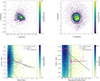 |
Fig. 7. Same as Figure 6 but for supergiants. |
| In the text | |
|
Fig. 8. Comparison of the radial metallicity gradients of the SMC (left) and the LMC (right) from this work with those from the literature. |
| In the text | |
|
Fig. A.1. Histograms of the LMC and SMC sources used for recalibration. On the top panel, the estimated photometric (Phot; blue) metallicities are plotted together with the spectroscopic (Spec; pink) metallicities as measured. On the bottom panel photometric metallicities are exploited after the addition of systematic difference. |
| In the text | |
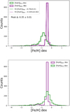 |
Fig. C.1. Same as Figure A.1 but for the supergiant sources. |
| In the text | |
|
Fig. C.2. Photometric [Fe/H] versus spectroscopic [Fe/H] of the RGB sources are shown on the top panel. The dotted line marks the one-to-one relation. In the bottom panel, photometric [Fe/H] (recalibrated with the slope and constant) is plotted against the difference between them. The colour bar from violet to green shows the increase in stellar density. |
| In the text | |
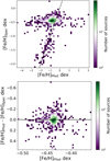 |
Fig. C.3. Same as Figure A.3 but for the supergiant sources. |
| In the text | |
|
Fig. D.1. Radial variation of Photometric versus Spectroscopic metallicities in RGB Stars of the Clouds. The top and middle rows display the peak differences between the photometric (Phot; blue) and spectroscopic (Spec; pink) RGB samples, calculated for various radial ranges from the centre of the LMC. The third row presents similar data for the RGB stars in the SMC. Both peaks are fitted, and the peak values are shown in the last row: on the left for the LMC and on the right for the SMC, which illustrates the radial variation of the shifts from the respective centres. |
| In the text | |
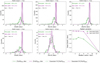 |
Fig. D.2. Same as Figure B.1 but for the LMC and SMC supergiant stars together. |
| In the text | |
|
Fig. D.3. Median error of [Fe/H] plotted against the number of sources in each bin for RGB (left) and supergiant (right) stars in the Clouds. Dotted vertical lines at 100 sources indicate the limit adopted in our study. |
| In the text | |
|
Fig. D.4. Maps showing the median error in the metallicity of RGB stars (left) and supergiants (right) of the Clouds. These maps are produced using the Voronoi binning method, where each bin has 100 sources. The colour-coding from purple to yellow indicates an increase in the median error. |
| In the text | |
|
Fig. D.5. Radial metallicity gradient (in degrees) for the RGB (top) and supergiant (bottom) stars for SMC (left) and LMC (right). In all panels, the increasing stellar density is colour-coded from purple to yellow. The median metallicities of the annular regions are marked with pink stars along with their standard errors. Linear best-fits and segmented best-fits are shown in green and grey, respectively. The black vertical lines show the division of different segments at the location of the breaks in the gradients. Underlying Hess diagrams show the source-density distributions. |
| In the text | |
Current usage metrics show cumulative count of Article Views (full-text article views including HTML views, PDF and ePub downloads, according to the available data) and Abstracts Views on Vision4Press platform.
Data correspond to usage on the plateform after 2015. The current usage metrics is available 48-96 hours after online publication and is updated daily on week days.
Initial download of the metrics may take a while.