| Issue |
A&A
Volume 700, August 2025
|
|
|---|---|---|
| Article Number | A171 | |
| Number of page(s) | 25 | |
| Section | Interstellar and circumstellar matter | |
| DOI | https://doi.org/10.1051/0004-6361/202553998 | |
| Published online | 15 August 2025 | |
Faint absorption of the ground state hyperfine-splitting transitions of hydroxyl at 18 cm in the Galactic disk★
1
National Radio Astronomy Observatory, PO Box O, Socorro, NM 87801, USA
2
Center for Astrophysics | Harvard & Smithsonian, 60 Garden Street, Cambridge, MA 02138, USA
3
Max Planck Institute for Radio Astronomy, Auf dem Hügel 69, 53121 Bonn, Germany
4
Max Planck Institute for Astronomy, Königstuhl 17, 69117 Heidelberg, Germany
5
Istituto di Astrofisica e Planetologia Spaziali (IAPS). INAF. Via Fosso del Cavaliere 100, 00133 Roma, Italy
6
Jet Propulsion Laboratory, California Institute of Technology, 4800 Oak Grove Drive, Pasadena, CA 91109, USA
7
Department of Physics and Astronomy, West Virginia University, Morgantown, WV 26506, USA
8
Center for Gravitational Waves and Cosmology, West Virginia University, Chestnut Ridge Research Building, Morgantown, WV 26505, USA
9
Adjunct Astronomer at the Green Bank Observatory, PO Box 2, Green Bank, WV 24944, USA
10
School of Physics, The University of Sydney, Physics Rd, Camperdown NSW 2050, Australia
11
School of Mathematical and Physical Sciences and Astrophysics and Space Technologies Research Centre, Macquarie University, 2109, NSW, Australia
12
Australia Telescope National Facility, CSIRO Space & Astronomy, PO Box 76, Epping, NSW 1710, Australia
13
Korea Astronomy and Space Science Institute, 776 Daedeok-daero, Daejeon 34055, Republic of Korea
14
Department of Astronomy and Space Science, University of Science and Technology, 217 Gajeong-ro, Daejeon 34113, Republic of Korea
15
Departamento de Astronomía, Universidad de la Serena, Raúl Bitrán 1305, la Serena, Chile
16
I. Physikalisches Institut, Universität zu Köln, Zülpicher Str. 77, 50937 Köln, Germany
17
Department of Astronomy & Astrophysics, University of California, San Diego, 9500 Gilman Drive, San Diego, CA 92093, USA
★★ Corresponding author: This email address is being protected from spambots. You need JavaScript enabled to view it.
Received:
3
February
2025
Accepted:
6
June
2025
Abstract
The interstellar hydride hydroxyl (OH) is a potential tracer of CO-dark molecular gas. We present new high-sensitivity absorption line observations of the four ground state hyperfine-splitting transitions of OH at 18 cm toward four Galactic and extragalactic continuum sources as follow-up to the THOR survey. We compared these to deep observations of the [C II] 158 µm line at 1.9 THz obtained with the upGREAT instrument on SOFIA, observations of the neutral atomic hydrogen (H I) 21 cm line with the VLA, and CO (J = 2–1) lines obtained with the APEX PI230 receiver at the APEX 12 m sub-mm telescope. We trace OH over a large range of molecular hydrogen column densities of 7.9 × 1019 cm-2 to 4.7 × 1022 cm-2, and derive OH abundances with respect to molecular and total hydrogen column densities of XOH,H2 = NOH/NH2 = 1.2−0.2+0.3 × 10⁻⁷ and XOH,H = NOH/NH = 4.8−0.8+0.9 × 10⁻⁸, respectively. Increased sensitivity and spectral resolution allowed us to detect weak and narrow features with the lowest column density detected at NOH = 3.7 × 1013 cm-2. The increase in sensitivity is a factor of five in direct comparison at the resolution the OH observations in the THOR survey (1.5 km s-1). We identify only one OH absorption component out of 23 without CO counterpart, yet several with intermediate molecular gas fractions (fmol ≤ 0.8). A potential association of [C II] 158 μm emission with an OH absorption component is seen toward one sightline. Our results confirm that OH absorption traces molecular gas across diffuse and dense environments of the interstellar medium. At the sensitivity limits of the present observations our detection of only one CO-dark molecular gas feature appears to be tracing only the upper end of the distribution of CO-dark OH features found by previous studies. We conclude that if OH absorption was to be used as a CO-dark molecular gas tracer, deeper observations or stronger background targets are necessary to unveil its full potential as a CO-dark molecular gas tracer, and yet it is not an exclusive tracer of CO-dark molecular gas. For OH hyperfine-splitting transitions in the vicinity of photodissociation regions in W43-South, we detect a spectral and spatial offset between the peak of the inversion of the OH 1612 MHz line and the absorption of the OH 1720 MHz line on the one hand, and the absorption of the OH main lines on the other hand, which provides additional constraints on the interpretation of the OH 18 cm line signatures typical of HII regions.
Key words: ISM: clouds / HII regions / ISM: molecules / Galaxy: abundances
This work is based on observations made with the Karl G. Jansky Very Large Array under the project VLA 17A-055. An earlier version of parts of this work appeared in the PhD thesis of M. R. Rugel.
M. R. Rugel is a Jansky Fellow of the National Radio Astronomy Observatory.
© The Authors 2025
 Open Access article, published by EDP Sciences, under the terms of the Creative Commons Attribution License (https://creativecommons.org/licenses/by/4.0), which permits unrestricted use, distribution, and reproduction in any medium, provided the original work is properly cited.
This article is published in open access under the Subscribe to Open model. This email address is being protected from spambots. You need JavaScript enabled to view it. to support open access publication.
1 Introduction
Molecular clouds are the birthplaces of stars. They form out of the diffuse atomic interstellar medium (ISM) once sufficient shielding from the interstellar radiation field is provided (e.g., Dobbs et al. 2014; Chevance et al. 2023; Pineda et al. 2023, and references therein), which also enables star formation (Glover & Clark 2012). Studying the formation of molecular clouds is essential for our understanding of star formation in the Milky Way.
Gas in cold molecular clouds consists mostly of H2. H2 emission from molecular clouds can be detected in shocks (e.g., Beckwith et al. 1983; Beuther et al. 2023, see also discussion in Sternberg 1989a) or by fluorescence emission (e.g., Sellgren 1986; Witt et al. 1989; Sternberg 1989b; Burkhart et al. 2025). Its rotational transitions with excitation energies about 500 K are impossible to be observed in emission under cold ISM conditions. Alternatively, such clouds are commonly studied with observations of the CO molecule (Wilson et al. 1970), whose low angular momentum (J) rotational lines are easily accessible at millimeter wavelengths. Several studies have indicated the presence of molecular gas not traced by CO emission (e.g., Grenier et al. 2005; Wolfire et al. 2010; Smith et al. 2014; Planck Collaboration XIX 2011). CO-dark molecular hydrogen gas, here defined as gas without detection of 12CO emission, has been found across the Galaxy at significant fractions (Pineda et al. 2013; Langer et al. 2014; Busch et al. 2021), in particular in regions of low extinction (Paradis et al. 2012; Xu et al. 2016; Remy et al. 2018). Observationally constraining the properties of “CO-dark” gas or simply “dark” gas thus contributes to our understanding of both the H CI-to-H2 conversion, as well as the onset of molecular cloud and star formation.
The ground state hyperfine-splitting (HFS) transitions of the hydroxyl molecule (OH) at centimeter wavelengths have been detected in regions with CO-dark gas. Xu et al. (2016) have investigated the relation between OH emission and dark gas fractions across the molecular cloud boundary in Taurus. Allen et al. (2015), Busch et al. (2019) and Busch et al. (2021) detected OH emission toward CO-dark lines-of-sight in the outer Galaxy, and Li et al. (2018) found OH absorption components without CO counterparts toward strong extragalactic continuum sources at high Galactic latitudes. Other detailed Galactic plane surveys investigating OH in emission across the Galactic plane include The Southern Parkes Large-Area Survey in Hydroxyl (SPLASH; Dawson et al. 2022). OH has also been found in high-mass star forming regions in association with photon-dominated/photo-dissociation regions (PDRs) and outflows (e.g., Goicoechea et al. 2011; Wampfler et al. 2011, 2013). The abundance of OH has been analyzed in several studies using the 18 cm lines (e.g., Goss 1968; Crutcher 1979; Liszt & Lucas 1996, 2002), with a detailed, recent studies of OH absorption presented in Hafner et al. (2023) and Nguyen et al. (2018). The OH abundance has also been investigated with the fundamental OH rotational transitions into the ground state at far-infrared wavelengths (Wiesemeyer et al. 2016; Jacob et al. 2022), as well as through its electronic transition at ultra-violett wavelengths (e.g. Weselak et al. 2010). Given that the OH hyperfine splitting transitions at 18 cm are readily accessible at ever higher resolution and sensitivity by today’s and future radio telescopes, a detailed study of OH in different Galactic environments seems warranted.
In this work, we present deep OH absorption observations along the lines of sight toward three bright background sources, as a follow-up study to The H I, OH, Recombination Line survey (THOR; Beuther et al. 2016; Wang et al. 2020), which observed the OH 18 cm lines over a large fraction of the first Galactic quadrant (Rugel et al. 2018; Beuther et al. 2019). We discuss the OH absorption toward four continuum sources which are chosen to be strong enough to reveal faint OH absorption from diffuse sightline clouds with typical optical depths of τ <0.1 (e.g., Dickey et al. 1981; Liszt & Lucas 1996), and increased spectral resolution as compared to THOR to resolve narrow absorption features. The field of view of one of the targets includes an extended H II region complex, which enabled additional studies of OH in PDRs (e.g., Brogan & Troland 2001) toward H II regions.
Furthermore, we searched for associated [C II] emission using observations carried out with the Stratospheric Observatory for Far-Infrared Astronomy (SOFIA; Young et al. 2012). [C II] emission can originate from different ISM environments, including the transition region between atomic and molecular gas. It has been used to estimate the CO-dark gas fraction in individual clouds (Xu et al. 2016), as well over the entire Milky Way disk (Pineda et al. 2013). [C II] emission has been detected in the diffuse ISM (Goldsmith et al. 2018), and may trace gas accretion onto molecular clouds (Heyer et al. 2022). [C II] is readily detected in absorption along the line-of-sight in clouds of varying molecular gas fractions (e.g., Gerin et al. 2015; Jacob et al. 2022).
The goal of this work is to characterize the abundance of the OH molecule in different ISM conditions. Of particular interest are the properties of the OH gas in diffuse ISM environments where CO becomes a less reliable tracer of the bulk molecular hydrogen content. We will present comparisons between [C II] emission and OH absorption. We additionally report findings on the excitation conditions of OH in H II regions.
2 Observations
2.1 VLA observations
We selected four continuum sources with a flux of ~1 Jy beam-1 (Fig. 1, Table 1). The H II region G29.957-0.018 has a spectral index1 of α = 0.9 (Wang et al. 2018), where positive spectral indices indicate thermal emission. G29.957-0.018 and G29.935-0.053 are part of the H II region complex W43-South, which has been attributed to the W43 complex (Motte et al. 2014). The continuum emission in W43-South at centimeter wavelengths has been presented in Beltrán et al. (2013), and the entire W43 complex is located at a distance of 5.49 kpc (Zhang et al. 2014). Two sources are of extragalactic origin (G21.347-0.629 and G31.388-0.383; with α = 0.0 and α = -0.9). All sources were selected based on OH absorption components in the THOR survey (Rugel et al. 2018) with weak (G29.957-0.018) or no (G31.388-0.383) 13CO (1-0) emission counterparts in the Galactic Ring Survey (GRS; Jackson et al. 2006).
We chose a channel width of 0.488 kHz (0.1 km s-1 at 1420 MHz), which is a significant improvement in comparison to the THOR survey (1.5 km s-1; Rugel et al. 2018). The bandwidth is 4 MHz for the H I and OH 1665/1667 MHz bands, and 2 MHz bands for the OH 1612 and OH 1720 MHz lines, which resulted in at least 300 km s-1 of usable bandwidth for the OH transitions (see Table 2 for frequencies discussed in this work). We observed for 8 nights between June and August 2017 with the VLA in C-configuration, with a total integration time of 7 h for G21.347-0.629, 4 h for G29.957-0.018 and G29.935-0.053, and 3h for G31.388-0.383. The observations were split into blocks of 2 h. We observed 3C286 for 10–20 minutes for bandpass calibration and used J1822-0938 as a complex gain calibrator.
We processed the observational data with the CASA2 calibration pipeline. We inspected the data for antenna and baseline artifacts. The calibrated data were imaged and de-convolved using the CASA task clean. We subtracted the continuum from line-free channels before imaging, and imaged spectral line cubes and continuum emission separately. The restoring beam is between 17″.2 × 12″.8 and 12″.8 × 11″.5. We smoothed all data to 18″ resolution (full width at half maximum, FWHM). The noise in a 0.2 km s-1 -wide channel is between 5 and 7 mJy beam-1 for the OH transitions. The increase in sensitivity is a factor of five in direct comparison at the resolution the OH observations in the THOR survey (10 mJy beam-1 at 1.5 km s-1 spectral resolution). For the H I line, the sensitivity is around 5 mJy beam-1 in a 0.5 km s-1-wide channel, corresponding to a brightness temperature of ~10 K. At velocities of Galactic HI emission, the noise increases up to a factor of two due to significant contributions of the H I emission to the system temperature.
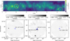 |
Fig. 1 Top: THOR 1.4 GHz continuum emission in the Galactic coordinate frame (Wang et al. 2020). The sources discussed here are located at the center of the yellow circles. Bottom: VLA 1.4 GHz continuum toward the four positions analyzed in this work (blue crosses) in equatorial coordinates. The images are smoothed to an angular resolution of 18″. |
Target locations and 1.4 GHz continuum fluxes.
2.2 SOFIA [C II] observations
We used the upGREAT receiver on the SOFIA telescope (Risacher et al. 2016) to measure the [C II] 158 µm line (see Table 2) toward G29.935-0.053 and G31.388-0.383. Due to observing time constraints, we were unable to obtain observations toward G21.347-0.629 and G29.957-0.018 was restricted to guaranteed time programs at the time of the proposal. The observations were conducted on June 8, 13, 19 and 20 of 2018 during flights from Christchurch, New Zealand, at an altitude of about 13 km as part of the project 06_0171 in position-switching total power mode. We used the standard SOFIA GREAT data reduction pipeline kalibrate. The spectra were corrected for atmospheric absorption.
The SOFIA upGREAT instrument consists of an array of 7 receivers (“pixels”) which observe simultaneously, and comprises two frequency channels operating at 1.9 and 4.7 THz, respectively. The low-frequency array was tuned to 1.9 THz to cover the [C II] 158 µm line, with an angular resolution of 14″.1. The high-frequency array was tuned to 4.7 THz to cover the [O I] 63 µm line (see Table 2), with an angular resolution of 6″.3. The data were calibrated with a forward efficiency of ηf = 0.97 and a main-beam efficiency which varies among the pixels between 0.55 and 0.70. As [C II] 158 µm emission extends to high Galactic latitudes, we chose two separate reference positions for both sources, identified as regions with low CO emission and low dust opacity using data from the Planck mission (Planck Collaboration XIX 2011 ; Planck Collaboration XI 2014) in absence of large scale maps of [C II] 158 µm emission. The time on each source was equally shared between the on-target position (50%) and two reference positions (25% each).
Pixel 2 was only available in vertical polarization, while all other pixels were observed in both linear polarizations. We note that pixel 4 shows higher baseline instabilities. Overall baselines were subtracted with first-order polynomials. For each pixel, we averaged all polarizations and observations with different reference positions. Similar steps have been applied for the [O I] 63 µm line, for which only the vertical polarization orientation was available. In the end, we averaged all available polarizations and spectra obtained with different reference positions. The final RMS on main beam temperature scales in the central pixel is σ(Tmb) ~ 0.1 K in a 0.39 km s-1 channel for the [C II] 158 μm, and ~0.2 K in a 0.15 km s-1 channel for the [O I] 63 μm spectra. Residual baseline ripples are present in both lines at a low level. We flagged any remaining channels with potential contamination from emission in the reference position, and disregarded them in the following analysis. All SOFIA upGREAT spectra are shown in Appendix B.
For G29.935-0.053, we searched for the [13C II] line. While we see indications of the F=1–0 line, the F=0–1 line is blended with the [C II] 158 µm line, and the F =1–1 line remains undetected. The velocity of the faint [13C II] F=1–0 line aligns with the velocity of a potential [C II] 158 µm self-absorption dip in many of the pixels. Due to overlap in velocity with the complex [C II] 158 µm emission along the line of sight across the Galaxy, a clear identification of the [13C II] F=1–0 remained difficult.
Spectral lines discussed in this work.
2.3 CO observations with the APEX telescope and from archival data
We observed the J =2-1 lines of different isotopologs of the CO molecule with the PI230 instrument on the Atacama Pathfinder EXperiment (APEX) 12 m submillimeter telescope (Güsten et al. 2006) for the sources for which we had obtained SOFIA [C II] 158 µm observations, G31.388-0.383 and G29.935-0.053. We observed both sources in position-switching mode. The tuning frequencies were chosen to cover the 12CO, 13CO, and C18O isotopologs, as well as the H30α radio recombination line. The CO lines have been resampled to a spectral resolution of 0.2 km s-1. The Tmb sensitivity is 0.04 K. To probe similar scales among different isotopologs, the observations were convolved to an angular resolution of 31″ (FWHM) from a resolution of 27″.1 for 12CO(2-1) and 2874 for 13CO (2-1) and C18O (2-1), respectively.
For G21.347-0.629 and G29.957-0.018, we used archival CO observations from three surveys. 13CO(1–0) observations were obtained from the GRS survey (Jackson et al. 2006). The GRS survey maps have a half-power beam width of 46″, and we corrected all data for a main-beam efficiency of ηmb = 0.48. Also, we used maps of 12CO(1–0) and C18O(1–0) emission from the FOREST Unbiased Galactic plane Imaging survey with the Nobeyama 45-m telescope (FUGIN) at 0.65 km s-1 spectral resolution (Umemoto et al. 2017), after convolving them from their original angular resolution of 20″ (FWHM) to 46″.
3 Analysis
3.1 OH and H I column densities
We determined the column density of OH from the 1667 MHz line, as its optical depth tends to be higher than the 1665 MHz line, thus likely being detected at a better signal-to-noise for a given excitation temperature. We estimated the optical depth of the H I and OH lines using  , with Fline corresponding to the flux density of the spectral line without continuum subtraction, Fcont the continuum flux density and τ the optical depth. The continuum was derived from the absorption-free channels. Given the strong continuum, we assumed that H I and OH emission is a negligible contribution to the spectrum after filtering extended emission with the interferometer. For saturated H I absorption channels, we calculated a lower limit on the optical depth by assuming a minimum H I absorption depth at the 3-σ noise level.
The OH excitation temperature is typically within a few Kelvin of the cosmic microwave background temperature (Li et al. 2018; Hafner et al. 2023), with a distribution up to higher values found up to Tex = 20 K. We fixed the excitation temperature at Tex = 5 K and accounted for an uncertainty of a factor of two for the excitation temperature in the error analysis. The OH column density was then calculated as:
 (1)
(1)
where NOH describes the total OH column density in particles cm-2 integrated over the optical depth profile in velocity, Tex is the excitation temperature in Kelvin, and the pre-factors are given as C0 = 4.0 × 1014 cm-2 K-1km-1s for the 1665 MHz line and C0 = 2.24 × 1014 cm-2 K-1km-1s for the 1667 MHz line (e.g., Goss 1968; Turner & Heiles 1971; Stanimirovic´ et al. 2003, calculated using Einstein coefficients from Turner 1966). For the filling factor we assumed f = 1.
Similarly, we derived the H I column densities using
 (2)
(2)
We assumed an average spin temperature of the absorbing H I gas of Tspin = 100 K, as the absorption is dominated by the cold neutral medium. We estimated the uncertainties in this assumption to be about a factor of two, given the significant spread in the distribution found in previous studies (e.g., Heiles & Troland 2003; Murray et al. 2018; Dickey et al. 2022).
We used NOH and NHI from the THOR survey for additional absorption features, and adopted a uniform excitation temperature for NOH of Tex = 5 K, for uniformity with the data presented here.
3.2 Molecular hydrogen column densities
For all but one line-of-sight OH absorption feature we detect 12CO rotational lines (see Table A.1), and used these to infer the molecular gas content. We converted integrated 12CO emission to molecular gas column density with a standard conversion factor of αCO = 2 × 1020 cm-2 (Bolatto et al. 2013). We rescaled the 12CO J = 2 - 1 observations by a typical line ratio of R21/10 = 0.7 (Sakamoto et al. 1997; Peñaloza et al. 2018; den Brok et al. 2021).
While a large fraction of the line-of sight OH absorption features show detections in the 13CO (1–0) line, we decided to rely exclusively on a 12CO conversion factor to derive molecular gas column densities. This choice was made as the rotational levels of weak 13CO (1–0) detections are likely sub-thermally excited (e.g., Heyer et al. 2006). Previous studies have found that the molecular gas column densities derived from 13 CO emission at low densities may be underestimated when assuming local thermal equilibrium (LTE) conditions (Goldsmith et al. 2008; Heyer et al. 2009; Heiderman et al. 2010). We tested deriving NH2 from the GRS 13CO (1–0) line emission reported here under LTE conditions (assuming Tex = 10 K), and found that NH2 was systematically lower by a factor of two or more for most but the highest column densities when comparing it to NH2 derived directly from 12CO emission. We hence adopted the NH2 values derived from 12CO emission. The integrated emission from all spectral lines is reported in Table A.1 to enable more refined modeling in future studies (e.g., Roueff et al. 2021).
For comparison with the THOR survey, we retrieved 12CO(1–0) spectra from the FUGIN survey to update the NH2 estimates for the following line-of-sight absorption features from Rugel et al. (2018): THOR+28.806+0.174+79.5, THOR+31.242-0.110+79.5, THOR+31.242-0.110+83.5, THOR+39.565-0.040+24.0, and THOR+42.027-0.604+64.5. As described in Rugel et al. (2018), all data were convolved to 46″ before extracting the spectra at the source position.
The NH2 estimates for OH absorption features associated with H II regions were adopted from Rugel et al. (2018), which used an excitation temperature of Tex = 20 K for the GRS 13CO (1–0) transition, applied an optical depth correction, and a standard conversion factor of N (H2) ~3.8 × 10⁵ N (13CO) (Pineda et al. 2008; Dickman 1978; Bolatto et al. 2013, and references therein). Given that the conversion does not account for the varying isotope ratio of 12C/13C with Galactocentric radius, we used the relation presented in Jacob et al. (2020) to rescale NH2 for OH absorption features within the solar circle. The Galactocen-tric radius was derived using parameters of the Galactic rotation curve from Reid et al. (2019), as used in the bayesian distance calculator3 (Reid et al. 2016). As the feature at 99.0 km s-1 for G29.935-0.053 presented in this work is associated with an H II region, we used the GRS 13CO (1–0) emission, following the same procedure as described above. We excluded any OH absorption associated with the H II region in G29.957-0.018, as the OH 1665 MHz transition is showing maser emission, which may affect the overall level population of the OH hyperfine splitting levels. After careful examination of the data, we used the 12CO(1–0) emission as described above also for THOR+32.272-0.226+22.5, as the column density from GRS 13CO (1–0) was severely underestimated.
Bolatto et al. (2013) estimated the uncertainties for αCO as 30%. Given that αCO and R21/10 may vary across the Milky Way, in particular in the diffuse ISM, the actual uncertainties in our sample are likely higher. We adopted an uncertainty for NH2 of a factor of 2.
4 Results
4.1 OH line-of-sight absorption
All but one of the OH absorption features are detected in 12CO, 18/23 in 13CO, and 5/23 in C18O. Detection of 12CO alone typically indicates gas at lower densities, while the detection of C18O requires dense gas. 3/23 features are associated with molecular gas in the vicinity of H II regions (see Table A.1), the other 20/23 features represent line-of-sight absorption. To derive column densities we measured integral properties of all spectral lines over 23 different intervals in velocity. An example for OH in low-density environments is the component at v = 37.0 km s-1 toward the extragalactic source G31.388-0.383. It is only weakly detected in 12CO (2–1) emission. An example for OH absorption associated with dense gas as traced by C18O is the deep OH absorption component at 56.5 km s-1 toward G21.347-0.629. The H I profile is also saturated here. We detect super-position of velocity components of low- and high-density gas: The OH 1667 MHz absorption feature along the line of sight toward the extragalactic source G21.347-0.629 at 55 km s-1 (Fig. A.1) shows a combination of a narrow component (Δv ~0.9km s-1) with a broader component (Δv ~6 km s-1), with their velocity centroids clearly shifted with respect to each other. The narrow and deeper component is detected in all CO isotopologs, and its detection in C18O clearly indicates the presence of dense gas in this narrow component. The broad component is detected only in the 12CO and 13CO lines, which indicates gas of lower density. Toward v =7 km s-1, a narrow component with a linewidth of 0.7 km s-1 in OH 1667 MHz absorption and 13CO emission is set on top of a broader component with a line width of 5.7 km s-1, which is weak but detected in OH 1667 MHz absorption and readily visible in 12CO emission.
Population inversion is a common feature in ground state HFS transitions of OH, particularly in its satellite lines at 1612 and 1720 MHz. We detect 6/23 features simultaneously in both satellite lines, of which three show conjugate behavior of stimulated emission in the OH 1612 MHz line and absorption in the OH 1720 MHz line. One shows the reverse configuration of absorption in the OH 1612 MHz line and stimulated emission in the OH 1720 MHz line, and two show absorption in both main lines. The remaining features show typically weak absorption in either the 1612 or the 1720 MHz line at the detection limit. Our sample does not contain clearly ‘flipped’ features which transition from emission to absorption, or vice versa, with increasing velocity, as has been described by Hafner et al. (2020). We note conjugated satellite line peaks toward G29.935-0.053 at v = 101.2 km s-1, which are shifted from the peak velocity of the main lines at 99 km s-1. However, we do not significantly detect a reversed feature at lower velocities. Figure A.1 indicates a potential reversal of the satellite lines across the broad velocity component at v = 7 km s-1 toward G21.347-0.629.
An example of OH main line inversion, which is typically seen in high-mass star forming regions (e.g., Beuther et al. 2019) pumped by strong infrared emission (e.g., Guibert et al. 1978) can be seen toward G29.957-0.018, in the components around 100 km s-1 which is associated with an UCH II region. Maser emission in the OH 1665 MHz line is visible between 100 and 105 km s-1 . Both main lines show maser emission at ~107 km s-1(Fig. A.2).
To summarize, we find that absorption in the OH 1665 MHz and OH 1667 MHz lines occurs in diffuse to dense environments. In the following sections, we discuss the OH abundance in these different ISM conditions.
4.2 The OH abundance in atomic and molecular gas
Given the occurrence of OH absorption in different ISM conditions noted in Sect. 4.1, this section analyzes the relation between OH absorption and tracers of different ISM gas phases. We traced the atomic gas component with the simultaneously recorded H I 21 cm line absorption. To trace phases dominated by molecular hydrogen we made use of new and archival observations of CO. Both approaches have limitations – the H I 21 cm line saturates at high column densities, while CO may be less abundant or not present at all at low molecular hydrogen abundances. As CO emission is one of the most commonly used tracer of molecular gas in the literature, we adopted CO as our reference tracer of molecular hydrogen, and discuss limitations and implications below.
The probed ranges of NOH and NH2 extend to lower column densities than in the THOR sample. The OH observations in this study extend to column densities as low as 3.7 × 10¹³ and up to 8.5 × 1014 cm-2. After rescaling NOH to the same excitation temperature as the data presented here, the OH observations in THOR4 (Rugel et al. 2018) probed higher column densities between 1.2 × 10¹⁴ and 3.8 × 1015 cm-2. The column densities of molecular hydrogen as probed in this work by CO emission extend from NH2 =7.7 × 10¹⁹ to 6.0 × 1022 cm-2, whereas the OH detections reported in Rugel et al. (2018) occur at NH2 =7.9 × 10²⁰ to 4.7 × 1022 cm-2.
In the following, we jointly analyzed both datasets. Due to higher sensitivities and higher spectral resolution (channel width of 0.2 versus 1.5 km s-1 for THOR) we were able to identify narrower features in the new sample presented here.
Figure 3 compares the OH column densities to the column density of atomic hydrogen and CO-derived molecular hydrogen, as well as to the total column density of hydrogen nuclei, which is given as NH = 2 × NH2 + NHI. Comparing with the column density of atomic hydrogen, we see that the H I absorption is saturated for all OH features with NHI > 1.4 × 1021 cm-2. We identified 12 features in the dataset presented in this work for which the H I absorption is not saturated.
The middle panel compares NOH with the column density of molecular hydrogen as traced by CO. The H2 column densities are estimated from different isotopologs as well as different rotational transitions of CO (see Sect. 3.2). One feature in the new dataset does not have a counterpart in any CO line, namely the feature at 68.8 km s-1 toward G21.347-0.629. To investigate the relationship between OH and molecular hydrogen column densities, we fitted the data with a power-law. To improve on previous estimates in Rugel et al. (2018) and to mitigate biases toward sublinear trends, we fitted a slope in logarithmic space with a least squares algorithm while properly accounting for uniform errors in both x and y directions, respectively (York 1966). We find the quantities to be related by a power law  with index mH2 = 1.0 ± 0.1. In the panel on the right-hand side of Fig. 3, we compare the OH column density to the total column density of hydrogen nuclei. Since the H I column density saturates in many instances, also NH is a lower limit. If we take only the 12 data points for which NHI is not saturated, the Spearman’s rank coefficient is rs = 0.6 with p = 0.08, which indicates that we cannot reject the null hypothesis at the present sample size. If we assume that the contribution of NH2 to NH dominates in most cases where NHI saturates, we can also consider NH estimates with saturated H I absorption. In this case we find an exponent for a power-law relation between NOH and NH of mH = 1.2 ± 0.1.
We investigated the OH abundance with respect to atomic, molecular and total hydrogen column density in Fig. 4. The median OH abundance with respect to molecular hydrogen is  . The upper and lower bounds indicate 16 and 84% confidence intervals of the abundance after bootstrapping the posterior distribution of the median over the error margins indicated in Sect. 3.2 (0.3 dex in NOH, NH2, and NHI). The median abundance with respect to the total column density of hydrogen nuclei is
  , omitting features with saturated H I lines. The sample with non-saturated H I column densities spreads a large range in molecular gas fractions (see Fig. 5). This holds true if we assume a lower spin temperature for NHI (Fig. A.4). Sources with saturated H I column densities tend to occur in line-of-sight features with high molecular gas fraction, and the lower limits of NHI would need to underestimate it by a factor of a few to significantly lower the molecular gas fractions. Including all estimates of NH, the median abundance is
  , which is just slightly higher than the result with H I detections only.
The abundances for line-of-sight components are  and
and  . This is slightly lower than the abundances for OH associated with H II regions which are
  and
and  . Figure 6 shows the molecular and total hydrogen abundance versus Galactocentric radius. While slight variations may be present, the Spearman’s rank test yielded p > 0.1 for any correlation between XOH,H2 or XOH,H and RGC, both for line-of-sight components and molecular clouds associated with H II regions individually, as well as all data combined.
4.3 Detections of the [C II] 158 µm emission toward OH absorption components
The [C II] observations for G31.388-0.383 and G29.935-0.053 are shown in Figs. 2 and A.3, respectively. We find widespread [C II] emission in both spectra originating from different velocity components along the line of sight. Given its strength and velocity, the main component of the [C II] emission in G29.935-0.053 is dominated by PDR emission from the H II region complex. G31.388-0.383 shows enhanced [C II] emission around 100 km s-1 and is affected by contamination in the reference position between 73 and 93 km s-1 (Fig. B.2). Below, we discuss [C II] emission as it occurs in conjunction with OH main line absorption.
For G29.935-0.053, Fig. A.3 does not show [C II] 158 μm emission that can be uniquely associated with line-of-sight OH absorption. While the [C II] 158 μm emission at v = 51 km s-1 is close in velocity to an OH absorption feature, its peak does not match, but rather seems to be associated with the deep H I absorption feature, as it spans a similar range in velocity. The lower emission between 0 and 30 km s-1 appears to be consistent between different observing dates and reference positions, and is seen in all of the pixels (Fig. B.5). It could indicate absorption, although we note baseline ripples of similar strength. As a confident estimate of the continuum level was not possible, we do not discuss the feature here further.
For G31.388-0.383 (Fig. 2), we see broad [C II] 158 μm emission toward v = 37 km s-1. However, we cannot identify a specific [C II] 158 µm emission feature associated in velocity with the OH absorption. Toward v = 18 km s-1 we detect significant [C II] 158 µm emission which is potentially associated with OH absorption. We discuss its gas content below. After removing contributions from the underlying broader emission profile, the component at 18km s-1 yields an integrated [C II] 158 μm emission of 1.8 Kkm s-1.
We estimated the column density of the [C II] 158 µm emission, re-arranging Equation (26) for the optically thin case from Goldsmith et al. (2012) (see also Beuther et al. 2022):
![Mathematical equation: \begin{aligned}N_{\rm CII} = \;& 2.9\times10^{15} \times \left[1+0.5{e}^{(91.25/T_{\rm kin})}\times\left(1+\frac{2.4\times10^{-6}}{n R_{ul}}\right)\right] \\ & \times \int T_{\rm mb} {\rm d}{v}\\\end{aligned}](/articles/aa/full_html/2025/08/aa53998-25/aa53998-25-eq14.png) (3)
(3)
We assumed a kinetic temperature of Tkin = 100K, a collision rate coefficient5 of Rul = 5 × 10⁻¹⁰ for collisions with ortho- and para-H2 (4.7 × 10⁻¹⁰ and, respectively, 5.5 × 10⁻¹⁰; Schöier et al. 2005; Lique et al. 2013) in an equal ratio, and densities of n = 103 cm-3. We find the column density to be NC+ = 4.3 × 1016cm-2.
In Sect. 3.2, we derived the H2 column density from the integrated 12CO emission directly. Here, we estimated the 12CO column density from its J=2–1 emission with an excitation temperature of Tex = 10 K using equation 79 in Mangum & Shirley (2015), and obtained N12CO = 7.1 × 1015cm-2. While we do not have tracers of neutral carbon available, this indicates considerable ionization fractions, consistent with models of translucent clouds (van Dishoeck & Black 1988). We note that the 1667 MHz OH absorption appears to consist of multiple components. A narrow one, which is detected in both 12CO and 13CO emission, as well as a broader one, which is only detected in 12CO. The 13CO emission has a line width of 1.2 km s-1, which is considerably narrower than the [C II] 158 µm emission with a FWHM of 3.7 km s-1. It may be that OH is picked up from both a diffuse, broad component with high carbon ionization fraction, as well as a denser, predominantly molecular component.
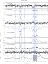 |
Fig. 2 OH and H I absorption toward the extragalactic source G31.388-0.383. The first five panels show optical depths of the four OH lines and H I, as derived from the line-to-continuum ratio. For the H I absorption, blue triangles indicate saturated channels. Emission spectra of the three CO isotopologs are shown below that. The data was taken with APEX and from the GRS (Jackson et al. 2006) survey. The lowest panel displays the SOFIA/upGREAT observations of the [C II] 158 µm line. Integration limits are shown as blue vertical lines. To emphasize that the OH and the H I lines were observed toward strong background sources, and are – with the exception of stimulated emission – seen in absorption, the axis of the optical depth is inverted, i.e., goes from positive to negative values. |
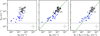 |
Fig. 3 OH column density vs. the column density of H I (left), H2 (middle), and the column density of the total number of hydrogen nuclei (right). Features associated with line-of-sight absorption are shown in blue, features associated with H II regions in black (Rugel et al. 2018). The middle panel shows NOH vs. NH2. Lower limits in case of saturated H I absorption in the left and right plots are indicated by triangles pointing to the right. There is one upper limit due to the non-detection of CO, which is indicated by triangles pointing to the left. Typical error bars are indicated in the lower right corner. The limit of a 3σ detection is indicated by a dashed gray line. The green dashed line indicates the fit of a correlation to the data. |
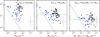 |
Fig. 4 Same as Fig. 3, but for the column density-averaged OH abundance. The dashed gray line indicates 3σ sensitivity limits of the OH absorption observations presented here. The green lines indicate the median abundance (solid) and 1σ uncertainties (dashed). |
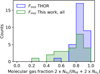 |
Fig. 5 Distribution of the molecular gas fraction in this work (green) in comparison to the sample from THOR (blue). Many of the features included in both samples are upper limits on the molecular gas fraction, as the H I absorption saturates. |
4.4 C in the H II region complex G29.935-0.053
The [C II] 158 μm emission associated with G29.935-0.053 shows complex line shapes, potentially affected by selfabsorption (Fig. A.3). Figure 7 shows the radio continuum emission at 1.4 GHz in contours across G29.935-0.053, together with the positions observed during the SOFIA observations. Pixel 0 (see Sect. 3.1) and pixel 5 are associated with peaks of the centimeter continuum emission, while the other pixels sample different parts of the HII region complex. The complete data are presented in Fig. A.5.
The [C II] 158 µm emission at pixel 0 extends between 76 and 127 km s-1 and contains three distinguishable emission peaks. The [O I] 63 µm emission shows a similar line shape (Fig. B.1). Recent studies have interpreted [C II] 158 and [O I] 63 µm emission from H II region complexes as a complex interplay of warm background emission and cold foreground absorption (Guevara et al. 2020, 2024), motivated by simultaneous detections of [13C II] and the [O I] 145 µm emission, which are typically optically thin and dominated by the warm background emission. No measurements of the [O I] 145 µm emission were available for this study. A search for [13C II] emission shows faint features at the correct velocities, but remains in the end inconclusive: the upGREAT SOFIA observations in the rest frame of the [13C II] F=1–0 and [13C II] F=1–1 lines (Fig. B.6) indicates an emission peak at rest velocities of G29.935-0.053 in the [13C II] F = 1-0 line, but it is over-posed by potential absorption, baseline ripples, and Galactic emission. The [13C II] F=1–1 line, located at lower frequencies than the [C II] 158 µm line, is the weakest of the three hyperfine splitting transitions and only shows marginal emission. Without a clear identification of the [13C II] hyperfinesplitting transitions and no availability of the [O I] 145 µm, the background and foreground components contributing to the [C II] 158 µm and the [O I] 63 µm cannot be disentangled.
We point out that the 12CO emission bears resemblance to the three-peak structure of the [C II] 158 µm emission. To some extent this also holds for the 13CO emission. Both show a trough at similar velocities as the [C II] 158 µm profile. The strongest peak of the C18O emission is aligned with the trough in the 12CO and 13 CO emission, indicating the presence of dense gas in this component, and suggesting that 12CO and 13CO lines are both optically thick at these velocities. This dense gas component also matches the velocity of the main line OH absorption peak. The C18O line shows several other peaks, both at lower velocities toward 93 km s-1, and at higher velocities at 102 km s-1 and 110 km s-1. The feature at 102 km s-1 falls into the red tail of the OH main line absorption feature. Given the alignment of the OH absorption, the C18O emission, and the trough in [C II] 158 µm emission over many of the pixels of the SOFIA observation (Fig. A.5), the trough in the [C II] 158 µm and the [O I] 63 µm emission may correspond to absorption of a colder foreground component. Additional observational constraints, however, are necessary to resolve the geometry of the region giving rise to the observed line profiles.
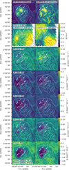 |
Fig. 7 Distribution of VLA 18 cm and GLIMPSE 8 µm continuum emission (top row Benjamin et al. 2003) in G29.935-0.053, with contours of ATLASGAL 870 µm emission (black; at 0.5, 1.0, 1.5 and 2 Jybeam-1 Schuller et al. 2009) and VLA 18 cm continuum (white; in steps of 0.1 Jy beam-1, starting at 0.03 Jy beam-1). The beam of both observations is indicated with a black circle in the lower left. The positions of the upGREAT LFA pixels are indicated, and the beamsize shown in blue. The following rows show spectral lines integrated over 95-100 km s-1 and 100-105 km s-1 in the left and right panels, respectively. |
4.5 Spatial and spectral variation in the OH excitation
Resolved 18 cm continuum observations in G29.935-0.053 enable us to investigate spatial and spectral variation in the excitation conditions of OH. Figure 7 indicates clumps of dense gas as traced by 870 µm emission from cold dust spatially surrounding 18 cm continuum emission. The Galactic Legacy Infrared Midplane Survey Extraordinaire (GLIMPSE) 8 µm map traces emission from poly aromatic hydrocarbons (PAHs) which appears to lie at interfaces between centimeter continuum emission and dust emission, indicating the location of PDR regions. The continuum emission toward pixels 0, 2, 3, 4 appears to lie behind a layer of molecular and atomic gas, as OH and H I is detected in absorption (Figure A.5). Radio recombination lines at 5 cm peak redshifted (toward pixels 2, 3, 4 and 5) or at similar velocities (pixel 0) as the OH absorption, indicating expansion away in the back of the molecular gas emission. Pixel 1 and 6 do not show OH absorption, indicating that the continuum emission may lie in front of the bulk of the molecular gas. The integrated C18O (2-1) emission between 95 and 100 km s-1 peaks toward the 870 µm emission peak, indicating that this velocity component may trace cold, dense molecular clumps. C18O (2– 1) emission at velocities between 100 and 105 km s-1 extends toward the southwest and northeast of the H II region.
The OH satellite lines peak at redder velocities than the minimum of the OH main line absorption and maximum of the C18O emission. This indicates the presence of distinct velocity components contributing to the OH lines, as also the CO emission in Fig. 7 appears to originate from different spatial locations inside G29.935-0.053 for different velocity ranges. Also, for the OH main lines, blueshifted components are strongest toward the peak of the continuum emission and close to the peak of the 870 µm emission. The peak of the redshifted component originates offset toward the northeast. The satellite line absorption (1720 MHz) and emission (1612 MHz) appear to follow the distribution of the redshifted component of the OH main line absorption.
5 Discussion
Section 4.1 indicates that gas at different densities contribute to OH absorption, as inferred from the detection statistics of CO isotopologs. This is in agreement with findings in the literature; for example, OH has been found in PDRs at densities of nH2 ~ 106 cm-3 (e.g., DR21; Jones et al. 1994; Koley 2023), and at intermediate to low densities in molecular cloud envelops of n < 103 cm-3 (TMC-1; Ebisawa et al. 2019). Busch et al. (2019) found an upper limit for the volume density of OH in CO-dark gas of n < 102 cm-3 through chemical modeling, and Busch et al. (2021) inferred extremely low average densities of as low as n ~ 7 × 10⁻³ cm-3 for a layer of CO-dark OH gas in the Outer Galaxy. The consistent appearance of OH throughout very different environments is likely related to its natural appearance in oxygen chemistry (e.g., van Dishoeck et al. 2013, and references therein), and the HFS transitions of the rotational ground state of OH are easily excited due to their small energy difference.
The initial motivation for this study was to follow-up and search for OH features which are candidates for tracing CO-dark gas as a potential tracer for the transition regions between atomic and molecular gas. Our investigations only revealed one feature without a simultaneous detection of carbon monoxide, at least within the sensitivities and angular resolution of the data at hand. This detection rate appears to be tracing only the upper end of the distribution of CO-dark OH features from previous studies: Li et al. (2018) found two sources significantly above our 3σ limit of 3-4×1013 cm-2 without a counterpart CO detection (there are three more at our 3σ limit). Conversely, they also find several OH features at similar column densities which show CO counterparts. Both the sample presented here and the THOR sample indicate OH absorption features at intermediate molecular gas fractions (<0.8; Fig. 5), i.e., for which the hydrogen gas content is not fully dominated by molecular hydrogen. These may fall into the diffuse molecular interstellar cloud type (Snow & McCall 2006). A particularly interesting feature in this context is the OH absorption feature at 37 km s-1 toward G31.388-0.383, which shows a highly elevated XOH,H2 but an average XOH,H value at RGC = 6.4 kpc in Fig. 6, indicating a large atomic gas fraction. We also note that αCO may be significantly underestimated at NH2 = 0.8 × 1020 cm-2 due to low CO abundances (van Dishoeck & Black 1988; Liszt 2007).
Our findings of a linear relation between NOH, NH2 and NH is in agreement with previous studies. Xu & Li (2016) find a linear relation between emission in the OH 1665 MHz line and dust extinction in the Taurus molecular cloud. Liszt & Lucas (1996) find OH absorption to be tightly correlated with HCO+. Our results show OH abundances which agree well with other measurements within the uncertainties and the scatter of our sample (e.g., Goss 1968; Crutcher 1979; Jacob et al. 2022; Albertsson et al. 2014). While the median abundance is slightly lower in more diffuse line-of-sight clouds than in dense molecular clouds associated within H II regions, they agree well within errors. We do not detect significant abundance variations with Galactocen-tric radius within the Solar circle. The measured abundances agree well with chemical models, which predict abundances between 10-8 and 10-7 for AV < 1, which can increase to ~10-6 for AV > 1 (e.g., Hollenbach et al. 2009, 2012).
Toward high densities in star forming regions and in the presence of strong infrared radiation fields, the excitation structure of the OH hyperfine splitting transitions (e.g., Nguyen-Q-Rieu et al. 1976) may vary from diffuse clouds, as indicated by the maser emission in G29.957-0.018 around 100 km s-1. A combined modeling of the hyperfine splitting transitions of OH at 18 cm with absorption of the OH rotational transitions into the ground state at far-infrared wavelengths (e.g., Wiesemeyer et al. 2012; Jacob et al. 2022) can further constrain the excitation structure. For OH absorption and emission features associated with high-mass star formation, previous studies revealed significant pumping by the far infrared radiation field (e.g., Goicoechea & Cernicharo 2002; Csengeri et al. 2012).
The analysis of the OH abundance presented here relies on CO as tracer of the bulk molecular gas, as measurements of CO are readily available and provide the necessary spectral information. However, we acknowledge that this introduces biases in the presented analysis: at the low end, it likely underestimates the true H2 column density given the presence of significant fractions of CO-dark gas in diffuse ISM regions (e.g., Grenier et al. 2005; Pineda et al. 2013). This would imply slightly steeper relations than determined in Sect. 4.2. The abundance itself, however, does not show significant trends toward higher abundances at low H2 column densities (Fig. 4) after accounting for the scatter and the approximate sensitivity limit (gray dashed line in Fig. 4). Indeed, if CO was underrepresenting the H2 column density, an expectation could be that the OH abundance increases with increasing Galactocentric radius as we derive NH2 from the CO emission. While Pineda et al. (2013) indicated an increase in the CO-dark gas fraction by a factor of about three between RGC = 4 kpc and RGC = 8 kpc, our data do not show evidence for a significant trend of the OH abundance with Galactocen-tric radius, neither for OH in line-of-sight absorption features, nor for OH associated with star formation (Fig. 6). This indicates that potential contributions of CO-dark gas to NH2 may be of limited impact, at least for the data presented here. Nevertheless, a comparison also to more suitable molecular gas tracers in the diffuse ISM, i.e., 3D dust maps (e.g., Mullens et al. 2024), HCO+ (e.g., Rybarczyk et al. 2022; Kim et al. 2023) or hydride absorption (e.g., Jacob et al. 2022), may be beneficial to further assess the OH abundances in the regime where CO ceases to be a reliable molecular gas tracer.
While the [C II] 158 µm line has been used as a tracer of CO-dark gas (e.g., Pineda et al. 2013), not all of the emission is molecular-gas dominated (e.g., Franeck et al. 2018; Ebagezio et al. 2024). As we find OH in lines of sight which have low molecular gas fractions (Sect. 3.1), we note at the same time for G29.935-0.053 and G31.388-0.383 that not all of the [C II] 158 µm emission has clear molecular gas counterparts. Some of the extended [C II] 158 µm emission at velocities close to the main molecular gas velocities may be tracing molecular cloud assembly, as suggested in observations (Schneider et al. 2023), and simulations (Clark et al. 2019). Finding the line width of the [C II] 158 μm emission component to be Δν = 3.4km s-1 in G31.388-0.383 - broader than the main molecular component -may itself be a signature of molecular clouds in formation (Heyer et al. 2022). The feature is slightly stronger (Tmb,peak = 0.55 K) than previous detections of [C II] 158 µm emission in the diffuse ISM (Goldsmith et al. 2018). Some of the population of features with weak [C II] 158 µm emission may have hence been missed at our sensitivity of σ ~ 0.1 K, as well as due to line-of-sight confusion in velocity.
The OH observations toward G29.935-0.053 appear to resemble parts of the common phenomenon “satellite line reversal” seen in several H II regions (Hafner et al. 2020), which is an opposing pattern of the OH satellite lines where the OH 1612 MHz line changes from absorption to inversion with increasing velocity, while the OH 1720 MHz changes from inversion to absorption. Even though not all parts of the profile are significantly detected, the identified parts of the features are in agreement with this phenomenon. Also, incomplete detections of the full profile in the OH satellite lines appear to be common (Rugel et al. 2018). The resemblance with the global pattern makes the observed line profiles in G29.935-0.053 unlikely to be related to any geometrical alignments unique to this object. Hafner et al. (2020) attribute the OH 1612 MHz inversion layer to a quiescent gas component into which the H II region is expanding, while the blueshifted OH 1720 MHz inversion originates from shocked gas itself. A detailed account of such an expansion scenario has been given in M17, as presented in Pellegrini et al. (2007, see also Brogan & Troland 2001; Brogan et al. 1999), who find blueshifted OH and H I absorption tracing an expanding shell into the ambient ISM. The ambient gas is associated with a redshifted component. Spatially, M17 also shows arcs in H I and OH absorption associated with the expansion. Applied to G29.935-0.053, the extended redshifted component would represent the molecular medium the H II region is expanding into, while the blueshifted absorption would be associated with the expanding shell itself. Albeit no proper 3D model of the H II complex is available for a full confirmation, the scenario proposed by Hafner et al. (2020) seems to be largely in agreement with the observations found here. A potential caveat would be that the blueshifted OH absorption component appears to coincide with the velocity of the dense gas clump toward pixel 5, for which the blueshifted component could be associated with the dense molecular gas itself which the HII region is expanding into at one side, instead of being solely related to the expansion of the shell. A larger sample of resolved studies of OH absorption can shed further light on this problem.
6 Conclusion
We present high-sensitivity OH and H I absorption observations at centimeter wavelengths with the VLA toward four lines of sight. These are follow-up observations of the THOR survey, initially to investigate faint OH absorption from diffuse interstellar clouds and cloud envelopes, but which were found to also trace OH in high-mass star forming regions. For two lines of sight, we compared the OH lines with [C II] 158 µm emission observations from upGREAT at SOFIA, as well as deep CO (2 - 1) lines with the PI230 receiver at the APEX telescope.
We find OH absorption at 1665 and 1667 MHz in a variety of ISM environments, both associated with dense and diffuse gas, and with gas with intermediate and high molecular gas fractions. We detect one feature which is without a CO counterpart. We compared OH with hydrogen column densities as derived from CO and HI. Within our uncertainties we find NOH linearly correlated both with respect to NH, where this is the total hydrogen column density, with a fitted power-law exponent of mH = 1.2 ± 0.1, and with respect to NH2 (mH2 = 1.0 ± 0.1). The derived OH abundances,
 and
and  , agree well with previous studies within the uncertainties and scatter of our measurements.
We detect [C II] 158 µm emission at similar velocities as an OH absorption feature toward G31.388-0.383. The estimated column density of ionized carbon exceeds the column density of carbon monoxide, indicating that significant fractions of the carbon in this feature are ionized, although the fraction of the C+ gas associated with the OH absorption is not clear. Other associations with line-of-sight OH absorption are not detected or remain ambiguous. G29.935-0.053 shows [C II] 158 µm emission from PDRs in the H II region complex with indications of [C II] 158 µm self-absorption, which is potentially associated with OH absorption.
G29.935-0.053 shows spectrally varying excitation conditions in all four OH lines, which manifest themselves in different spatial morphologies of the optical depths of the OH satellite lines (OH 1612/1720 MHz) as compared to the main lines (OH 1665/1667 MHz). This confirms previous studies in that both OH absorption and stimulated emission can originate from multiple gas components in an H II region complex.
For the mid-plane of the Milky Way disk, we find that the detection of true CO-dark gas remains challenging. The relevance of the hyperfine splitting transitions of hydroxyl at 18 cm as tracer of the onset of molecular cloud formation is yet to be further explored. Ray-tracing of simulations, observations of the OH 18 cm lines with future radio telescopes, or complementary investigations of transitions of OH at other frequencies (e.g., Jacob et al. 2022, Busch et al., in prep.) can help to address this question.
Acknowledgements
We dedicate this work to Karl M. Menten, who significantly contributed to the present manuscript and sadly passed away before the submission of the paper. He was a brilliant and accomplished scientist, a mentor of the highest standard, and will be greatly missed. We would like to thank the anonymous referee for comments and suggestions which greatly improved this work. M.R.R. thanks several members of the MPIfR in Bonn, the Center for Astrophysics | Harvard & Smithsonian, and the HyGAL collaboration for discussions, in particular M. Reid, Q. Zhang, P. Myers, D. Neufeld, Brian Svoboda. The authors would like to thank the SOFIA and APEX teams for carrying out the observations, and the support in preparing them. The National Radio Astronomy Observatory and Green Bank Observatory are facilities of the National Science Foundation operated under cooperative agreement by Associated Universities, Inc. Based in part on observations made with the NASA/DLR Stratospheric Observatory for Infrared Astronomy (SOFIA). SOFIA is jointly operated by the Universities Space Research Association, Inc. (USRA), under NASA contract NNA17BF53C, and the Deutsches SOFIA Institut (DSI) under DLR contract 50 OK 2002 to the University of Stuttgart. The development and operation of GREAT was financed by resources from the participating institutes, by the Deutsche Forschungsgemeinschaft (DFG) within the grant for the Collaborative Research Center 956 as well as by the Federal Ministry of Economics and Energy (BMWI) via the German Space Agency (DLR) under Grants 50 OK 1102, 50 OK 1103 and 50 OK 1104. This research was conducted in part at the Jet Propulsion Laboratory, which is operated by the California Institute of Technology under contract with the National Aeronautics and Space Administration (NASA). This data made use of splatalogue, CDS, simbad, astropy, reproject, spectral-cube, aplpy, matplotlib, gildas, carta.
Appendix A Additional spectra and results
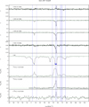 |
Fig. A.1 Same as Fig. 2, but toward G21.347-0.629. The CO data has been taken from the FUGIN (Umemoto et al. 2017) and GRS (Jackson et al. 2006) surveys. No [C II] 158 µm emission spectrum has been recorded for this source. |
OH, HI, and H2 column densities
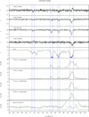 |
Fig. A.3 Same as Fig. 2, but for G29.935-0.053. The bottom panel includes an enlarged view of the [C II] 158 µm line for better visibility of the faint emission or absorption components, and/or baseline ripples. |
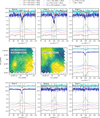 |
Fig. A.5 Optical depth of the OH lines at 1612, 1665, 1667 and 1720 MHz, as well of H I toward the seven pixels toward G29.935-0.053 of the upGREAT/SOFIA [12C II] observations, as well as accompanying C18O (2–1) (APEX/PI230) and stacked radio recombination lines (40″, GLOSTAR; Brunthaler et al. 2021; Khan et al. 2024). The maps in the middle panel are repeated for clarity from row 2 in Fig. 7. |
Appendix B Overview SOFIA data
 |
Fig. B.1 [O I] 63 µm emission toward G29.935-0.053. For each spectrum, we show the average of all data (black). We only show the [C II] 158 µm emission for reference in pixel 1, as the other pixels are closer to the central beam than for [C II] 158 µm and do not overlap. Offsets from the source position are indicated in arcsec. |
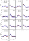 |
Fig. B.2 [C II] 158 µm emission toward G31.388-0.383. For each spectrum, we show the average of all data (black), as well as averages by reference position. Note that only vertical polarization (“V”) is available for Pixel 2. The gray-shaded region is masked as it is contaminated by emission in the reference position. |
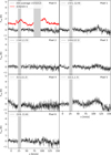 |
Fig. B.3 [O I] 63 µm emission toward G31.388-0.383. For each spectrum, we show the average of all data (black). We only show the [C II] 158 µm emission for reference in pixel 1, as the other pixels are closer to the central beam than for [C II] 158 µm and do not overlap. Several pixels show residual low-frequency baseline ripples. The gray-shaded region around 25 km s-1 is masked due to residual artefacts from atmospheric corrections. |
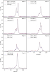 |
Fig. B.4 [C II] 158 µm emission toward G29.935-0.053. For each spectrum, we show the average of all data (black), as well as averages by reference position. Note that only vertical polarization (“V”) is available for Pixel 2. |
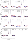 |
Fig. B.5 Zoom-in on the low-level [C II] 158 µm emission in G29.935-0.053. Colors and spectra as in Fig. B.4. |
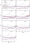 |
Fig. B.6 [C II] 158 µm and [13C II] emission toward G29.935-0.053. Colors and spectra as in Fig. B.4, with the spectra in each subplot shifted to the rest frequency of each line. |
References
- Albertsson, T., Indriolo, N., Kreckel, H., et al. 2014, ApJ, 787, 44 [Google Scholar]
- Allen, R. J., Hogg, D. E., & Engelke, P. D. 2015, AJ, 149, 123 [NASA ADS] [CrossRef] [Google Scholar]
- Beckwith, S., Evans, II, N. J., Gatley, I., Gull, G., & Russell, R. W. 1983, ApJ, 264, 152 [Google Scholar]
- Beltrán, M. T., Olmi, L., Cesaroni, R., et al. 2013, A&A, 552, A123 [Google Scholar]
- Benjamin, R. A., Churchwell, E., Babler, B. L., et al. 2003, PASP, 115, 953 [Google Scholar]
- Beuther, H., Bihr, S., Rugel, M., et al. 2016, A&A, 595, A32 [NASA ADS] [CrossRef] [EDP Sciences] [Google Scholar]
- Beuther, H., Walsh, A., Wang, Y., et al. 2019, A&A, 628, A90 [NASA ADS] [CrossRef] [EDP Sciences] [Google Scholar]
- Beuther, H., Schneider, N., Simon, R., et al. 2022, A&A, 659, A77 [NASA ADS] [CrossRef] [EDP Sciences] [Google Scholar]
- Beuther, H., van Dishoeck, E. F., Tychoniec, L., et al. 2023, A&A, 673, A121 [NASA ADS] [CrossRef] [EDP Sciences] [Google Scholar]
- Bolatto, A. D., Wolfire, M., & Leroy, A. K. 2013, ARA&A, 51, 207 [CrossRef] [Google Scholar]
- Brogan, C. L., & Troland, T. H. 2001, ApJ, 560, 821 [NASA ADS] [CrossRef] [Google Scholar]
- Brogan, C. L., Troland, T. H., Roberts, D. A., & Crutcher, R. M. 1999, ApJ, 515, 304 [Google Scholar]
- Brunthaler, A., Menten, K. M., Dzib, S. A., et al. 2021, A&A, 651, A85 [EDP Sciences] [Google Scholar]
- Burkhart, B., Dharmawardena, T. E., Bialy, S., et al. 2025, Nat. Astron. [arXiv:2504.17843] [Google Scholar]
- Busch, M. P., Allen, R. J., Engelke, P. D., et al. 2019, ApJ, 883, 158 [Google Scholar]
- Busch, M. P., Engelke, P. D., Allen, R. J., & Hogg, D. E. 2021, ApJ, 914, 72 [CrossRef] [Google Scholar]
- Chevance, M., Krumholz, M. R., McLeod, A. F., et al. 2023, ASP Conf. Ser., 534, 1 [NASA ADS] [Google Scholar]
- Clark, P. C., Glover, S. C. O., Ragan, S. E., & Duarte-Cabral, A. 2019, MNRAS, 486, 4622 [Google Scholar]
- Crutcher, R. M. 1979, ApJ, 234, 881 [Google Scholar]
- Csengeri, T., Menten, K. M., Wyrowski, F., et al. 2012, A&A, 542, L8 [NASA ADS] [CrossRef] [EDP Sciences] [Google Scholar]
- Dawson, J. R., Jones, P. A., Purcell, C., et al. 2022, MNRAS, 512, 3345 [NASA ADS] [CrossRef] [Google Scholar]
- den Brok, J. S., Chatzigiannakis, D., Bigiel, F., et al. 2021, MNRAS, 504, 3221 [NASA ADS] [CrossRef] [Google Scholar]
- Dickey, J. M., Crovisier, J., & Kazes, I. 1981, A&A, 98, 271 [NASA ADS] [Google Scholar]
- Dickey, J. M., Dempsey, J. M., Pingel, N. M., et al. 2022, ApJ, 926, 186 [NASA ADS] [CrossRef] [Google Scholar]
- Dickman, R. L. 1978, ApJS, 37, 407 [CrossRef] [Google Scholar]
- Dobbs, C. L., Krumholz, M. R., Ballesteros-Paredes, J., et al. 2014, in Protostars and Planets VI, eds. H. Beuther, R. S. Klessen, C. P. Dullemond, & T. Henning (Tucson: University of Arizona Press), 3 [Google Scholar]
- Ebagezio, S., Seifried, D., Walch, S., & Bisbas, T. G. 2024, A&A, 692, A58 [NASA ADS] [CrossRef] [EDP Sciences] [Google Scholar]
- Ebisawa, Y., Sakai, N., Menten, K. M., & Yamamoto, S. 2019, ApJ, 871, 89 [Google Scholar]
- Franeck, A., Walch, S., Seifried, D., et al. 2018, MNRAS, 481, 4277 [NASA ADS] [CrossRef] [Google Scholar]
- Gerin, M., Ruaud, M., Goicoechea, J. R., et al. 2015, A&A, 573, A30 [NASA ADS] [CrossRef] [EDP Sciences] [Google Scholar]
- Glover, S. C. O., & Clark, P. C. 2012, MNRAS, 421, 9 [NASA ADS] [Google Scholar]
- Goicoechea, J. R., & Cernicharo, J. 2002, ApJ, 576, L77 [NASA ADS] [CrossRef] [Google Scholar]
- Goicoechea, J. R., Joblin, C., Contursi, A., et al. 2011, A&A, 530, L16 [CrossRef] [EDP Sciences] [Google Scholar]
- Goldsmith, P. F., Heyer, M., Narayanan, G., et al. 2008, ApJ, 680, 428 [Google Scholar]
- Goldsmith, P. F., Langer, W. D., Pineda, J. L., & Velusamy, T. 2012, ApJS, 203, 13 [Google Scholar]
- Goldsmith, P. F., Pineda, J. L., Neufeld, D. A., et al. 2018, ApJ, 856, 96 [NASA ADS] [CrossRef] [Google Scholar]
- Goss, W. M. 1968, ApJS, 15, 131 [Google Scholar]
- Grenier, I. A., Casandjian, J.-M., & Terrier, R. 2005, Science, 307, 1292 [Google Scholar]
- Guevara, C., Stutzki, J., Ossenkopf-Okada, V., et al. 2020, A&A, 636, A16 [CrossRef] [EDP Sciences] [Google Scholar]
- Guevara, C., Stutzki, J., Ossenkopf-Okada, V., et al. 2024, A&A, 690, A294 [NASA ADS] [CrossRef] [EDP Sciences] [Google Scholar]
- Guibert, J., Rieu, N. Q., & Elitzur, M. 1978, A&A, 66, 395 [NASA ADS] [Google Scholar]
- Güsten, R., Nyman, L. Å., Schilke, P., et al. 2006, A&A, 454, L13 [NASA ADS] [CrossRef] [EDP Sciences] [Google Scholar]
- Hafner, A., Dawson, J. R., & Wardle, M. 2020, MNRAS, 497, 4066 [Google Scholar]
- Hafner, A., Dawson, J. R., Nguyen, H., et al. 2023, PASA, 40, e015 [Google Scholar]
- Heiderman, A., Evans, II, N. J., Allen, L. E., Huard, T., & Heyer, M. 2010, ApJ, 723, 1019 [NASA ADS] [CrossRef] [Google Scholar]
- Heiles, C., & Troland, T. H. 2003, ApJ, 586, 1067 [NASA ADS] [CrossRef] [Google Scholar]
- Heyer, M. H., Williams, J. P., & Brunt, C. M. 2006, ApJ, 643, 956 [NASA ADS] [CrossRef] [Google Scholar]
- Heyer, M., Krawczyk, C., Duval, J., & Jackson, J. M. 2009, ApJ, 699, 1092 [Google Scholar]
- Heyer, M., Goldsmith, P. F., Simon, R., Aladro, R., & Ricken, O. 2022, ApJ, 941, 62 [Google Scholar]
- Hollenbach, D., Kaufman, M. J., Bergin, E. A., & Melnick, G. J. 2009, ApJ, 690, 1497 [NASA ADS] [CrossRef] [Google Scholar]
- Hollenbach, D., Kaufman, M. J., Neufeld, D., Wolfire, M., & Goicoechea, J. R. 2012, ApJ, 754, 105 [Google Scholar]
- Jackson, J. M., Rathborne, J. M., Shah, R. Y., et al. 2006, ApJS, 163, 145 [NASA ADS] [CrossRef] [Google Scholar]
- Jacob, A. M., Menten, K. M., Wiesemeyer, H., et al. 2020, A&A, 640, A125 [EDP Sciences] [Google Scholar]
- Jacob, A. M., Neufeld, D. A., Schilke, P., et al. 2022, ApJ, 930, 141 [NASA ADS] [CrossRef] [Google Scholar]
- Jones, K. N., Field, D., Gray, M. D., & Walker, R. N. F. 1994, A&A, 288, 581 [NASA ADS] [Google Scholar]
- Khan, S., Rugel, M. R., Brunthaler, A., et al. 2024, A&A, 689, A81 [NASA ADS] [CrossRef] [EDP Sciences] [Google Scholar]
- Kim, W. J., Schilke, P., Neufeld, D. A., et al. 2023, A&A, 670, A111 [NASA ADS] [CrossRef] [EDP Sciences] [Google Scholar]
- Koley, A. 2023, PASA, 40, e046 [Google Scholar]
- Langer, W. D., Velusamy, T., Pineda, J. L., Willacy, K., & Goldsmith, P. F. 2014, A&A, 561, A122 [NASA ADS] [CrossRef] [EDP Sciences] [Google Scholar]
- Li, D., Tang, N., Nguyen, H., et al. 2018, ApJS, 235, 1 [Google Scholar]
- Lique, F., Werfelli, G., Halvick, P., et al. 2013, J. Chem. Phys., 138, 204314 [NASA ADS] [CrossRef] [Google Scholar]
- Liszt, H. S. 2007, A&A, 476, 291 [NASA ADS] [CrossRef] [EDP Sciences] [Google Scholar]
- Liszt, H., & Lucas, R. 1996, A&A, 314, 917 [Google Scholar]
- Liszt, H., & Lucas, R. 2002, A&A, 391, 693 [NASA ADS] [CrossRef] [EDP Sciences] [Google Scholar]
- Mangum, J. G., & Shirley, Y. L. 2015, PASP, 127, 266 [Google Scholar]
- Motte, F., Nguyen Luong, Q., Schneider, N., et al. 2014, A&A, 571, A32 [NASA ADS] [CrossRef] [EDP Sciences] [Google Scholar]
- Mullens, E., Zucker, C., Murray, C. E., & Smith, R. 2024, ApJ, 966, 127 [Google Scholar]
- Murray, C. E., Stanimirovic´, S., Goss, W. M., et al. 2018, ApJS, 238, 14 [NASA ADS] [CrossRef] [Google Scholar]
- Nguyen, H., Dawson, J. R., Miville-Deschênes, M. A., et al. 2018, ApJ, 862, 49 [NASA ADS] [CrossRef] [Google Scholar]
- Nguyen-Q-Rieu, Winnberg, A., Guibert, J., et al. 1976, A&A, 46, 413 [NASA ADS] [Google Scholar]
- Paradis, D., Dobashi, K., Shimoikura, T., et al. 2012, A&A, 543, A103 [NASA ADS] [CrossRef] [EDP Sciences] [Google Scholar]
- Peñaloza, C. H., Clark, P. C., Glover, S. C. O., & Klessen, R. S. 2018, MNRAS, 475, 1508 [CrossRef] [Google Scholar]
- Pellegrini, E. W., Baldwin, J. A., Brogan, C. L., et al. 2007, ApJ, 658, 1119 [NASA ADS] [CrossRef] [Google Scholar]
- Pineda, J. E., Caselli, P., & Goodman, A. A. 2008, ApJ, 679, 481 [Google Scholar]
- Pineda, J. L., Langer, W. D., Velusamy, T., & Goldsmith, P. F. 2013, A&A, 554, A103 [CrossRef] [EDP Sciences] [Google Scholar]
- Pineda, J. E., Arzoumanian, D., Andre, P., et al. 2023, ASP Conf. Ser., 534, 233 [NASA ADS] [Google Scholar]
- Planck Collaboration XI. 2014, A&A, 571, A11 [NASA ADS] [CrossRef] [EDP Sciences] [Google Scholar]
- Planck Collaboration XIX. 2011, A&A, 536, A19 [NASA ADS] [CrossRef] [EDP Sciences] [Google Scholar]
- Reid, M. J., Dame, T. M., Menten, K. M., & Brunthaler, A. 2016, ApJ, 823, 77 [Google Scholar]
- Reid, M. J., Menten, K. M., Brunthaler, A., et al. 2019, ApJ, 885, 131 [Google Scholar]
- Remy, Q., Grenier, I. A., Marshall, D. J., & Casandjian, J. M. 2018, A&A, 611, A51 [NASA ADS] [CrossRef] [EDP Sciences] [Google Scholar]
- Risacher, C., Güsten, R., Stutzki, J., et al. 2016, A&A, 595, A34 [NASA ADS] [CrossRef] [EDP Sciences] [Google Scholar]
- Roueff, A., Gerin, M., Gratier, P., et al. 2021, A&A, 645, A26 [NASA ADS] [CrossRef] [EDP Sciences] [Google Scholar]
- Rugel, M. R., Beuther, H., Bihr, S., et al. 2018, A&A, 618, A159 [NASA ADS] [CrossRef] [EDP Sciences] [Google Scholar]
- Rybarczyk, D. R., Stanimirovic´, S., Gong, M., et al. 2022, ApJ, 928, 79 [NASA ADS] [CrossRef] [Google Scholar]
- Sakamoto, S., Hasegawa, T., Handa, T., Hayashi, M., & Oka, T. 1997, ApJ, 486, 276 [NASA ADS] [CrossRef] [Google Scholar]
- Schneider, N., Bonne, L., Bontemps, S., et al. 2023, Nat. Astron., 7, 546 [NASA ADS] [CrossRef] [Google Scholar]
- Schöier, F. L., van der Tak, F. F. S., van Dishoeck, E. F., & Black, J. H. 2005, A&A, 432, 369 [Google Scholar]
- Schuller, F., Menten, K. M., Contreras, Y., et al. 2009, A&A, 504, 415 [NASA ADS] [CrossRef] [EDP Sciences] [Google Scholar]
- Sellgren, K. 1986, ApJ, 305, 399 [NASA ADS] [CrossRef] [Google Scholar]
- Smith, R. J., Glover, S. C. O., Clark, P. C., Klessen, R. S., & Springel, V. 2014, MNRAS, 441, 1628 [NASA ADS] [CrossRef] [Google Scholar]
- Snow, T. P., & McCall, B. J. 2006, ARA&A, 44, 367 [NASA ADS] [CrossRef] [Google Scholar]
- Stanimirovic´ , S., Weisberg, J. M., Dickey, J. M., et al. 2003, ApJ, 592, 953 [Google Scholar]
- Sternberg, A. 1989a, in Infrared Spectroscopy in Astronomy, ed. E. Böhm-Vitense (Cambridge: Cambridge University Press), 269 [Google Scholar]
- Sternberg, A. 1989b, ApJ, 347, 863 [Google Scholar]
- Turner, B. E. 1966, Nature, 212, 184 [Google Scholar]
- Turner, B. E., & Heiles, C. 1971, ApJ, 170, 453 [Google Scholar]
- Umemoto, T., Minamidani, T., Kuno, N., et al. 2017, PASJ, 69, 78 [Google Scholar]
- van Dishoeck, E. F., & Black, J. H. 1988, ApJ, 334, 771 [Google Scholar]
- van Dishoeck, E. F., Herbst, E., & Neufeld, D. A. 2013, Chem. Rev., 113, 9043 [Google Scholar]
- Wampfler, S. F., Bruderer, S., Kristensen, L. E., et al. 2011, A&A, 531, L16 [NASA ADS] [CrossRef] [EDP Sciences] [Google Scholar]
- Wampfler, S. F., Bruderer, S., Karska, A., et al. 2013, A&A, 552, A56 [NASA ADS] [CrossRef] [EDP Sciences] [Google Scholar]
- Wang, Y., Bihr, S., Rugel, M., et al. 2018, A&A, 619, A124 [NASA ADS] [CrossRef] [EDP Sciences] [Google Scholar]
- Wang, Y., Beuther, H., Rugel, M. R., et al. 2020, A&A, 634, A83 [NASA ADS] [CrossRef] [EDP Sciences] [Google Scholar]
- Weselak, T., Galazutdinov, G. A., Beletsky, Y., & Krełowski, J. 2010, MNRAS, 402, 1991 [NASA ADS] [CrossRef] [Google Scholar]
- Wiesemeyer, H., Güsten, R., Heyminck, S., et al. 2012, A&A, 542, L7 [NASA ADS] [CrossRef] [EDP Sciences] [Google Scholar]
- Wiesemeyer, H., Güsten, R., Heyminck, S., et al. 2016, A&A, 585, A76 [NASA ADS] [CrossRef] [EDP Sciences] [Google Scholar]
- Wilson, R. W., Jefferts, K. B., & Penzias, A. A. 1970, ApJ, 161, L43 [NASA ADS] [CrossRef] [Google Scholar]
- Witt, A. N., Stecher, T. P., Boroson, T. A., & Bohlin, R. C. 1989, ApJ, 336, L21 [NASA ADS] [CrossRef] [Google Scholar]
- Wolfire, M. G., Hollenbach, D., & McKee, C. F. 2010, ApJ, 716, 1191 [Google Scholar]
- Xu, D., & Li, D. 2016, ApJ, 833, 90 [Google Scholar]
- Xu, D., Li, D., Yue, N., & Goldsmith, P. F. 2016, ApJ, 819, 22 [NASA ADS] [CrossRef] [Google Scholar]
- York, D. 1966, Canad. J. Phys., 44, 1079 [Google Scholar]
- Young, E. T., Becklin, E. E., Marcum, P. M., et al. 2012, ApJ, 749, L17 [NASA ADS] [CrossRef] [Google Scholar]
- Zhang, B., Moscadelli, L., Sato, M., et al. 2014, ApJ, 781, 89 [Google Scholar]
The spectral index is defined as  , where S0 is the flux at a reference frequency, v0 at 1.4 GHz.
http://casa.nrao.edu; version 4.7.2; pipeline version 1.3.11.
v2.4.1.
OH absorption detections presented here were not removed from the original sample presented in Rugel et al. (2018).
All Tables
All Figures
|
Fig. 1 Top: THOR 1.4 GHz continuum emission in the Galactic coordinate frame (Wang et al. 2020). The sources discussed here are located at the center of the yellow circles. Bottom: VLA 1.4 GHz continuum toward the four positions analyzed in this work (blue crosses) in equatorial coordinates. The images are smoothed to an angular resolution of 18″. |
| In the text | |
|
Fig. 2 OH and H I absorption toward the extragalactic source G31.388-0.383. The first five panels show optical depths of the four OH lines and H I, as derived from the line-to-continuum ratio. For the H I absorption, blue triangles indicate saturated channels. Emission spectra of the three CO isotopologs are shown below that. The data was taken with APEX and from the GRS (Jackson et al. 2006) survey. The lowest panel displays the SOFIA/upGREAT observations of the [C II] 158 µm line. Integration limits are shown as blue vertical lines. To emphasize that the OH and the H I lines were observed toward strong background sources, and are – with the exception of stimulated emission – seen in absorption, the axis of the optical depth is inverted, i.e., goes from positive to negative values. |
| In the text | |
|
Fig. 3 OH column density vs. the column density of H I (left), H2 (middle), and the column density of the total number of hydrogen nuclei (right). Features associated with line-of-sight absorption are shown in blue, features associated with H II regions in black (Rugel et al. 2018). The middle panel shows NOH vs. NH2. Lower limits in case of saturated H I absorption in the left and right plots are indicated by triangles pointing to the right. There is one upper limit due to the non-detection of CO, which is indicated by triangles pointing to the left. Typical error bars are indicated in the lower right corner. The limit of a 3σ detection is indicated by a dashed gray line. The green dashed line indicates the fit of a correlation to the data. |
| In the text | |
|
Fig. 4 Same as Fig. 3, but for the column density-averaged OH abundance. The dashed gray line indicates 3σ sensitivity limits of the OH absorption observations presented here. The green lines indicate the median abundance (solid) and 1σ uncertainties (dashed). |
| In the text | |
|
Fig. 5 Distribution of the molecular gas fraction in this work (green) in comparison to the sample from THOR (blue). Many of the features included in both samples are upper limits on the molecular gas fraction, as the H I absorption saturates. |
| In the text | |
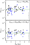 |
Fig. 6 Same as Fig. 4 but for XOH,H2 and XOH,H vs. RGC. |
| In the text | |
|
Fig. 7 Distribution of VLA 18 cm and GLIMPSE 8 µm continuum emission (top row Benjamin et al. 2003) in G29.935-0.053, with contours of ATLASGAL 870 µm emission (black; at 0.5, 1.0, 1.5 and 2 Jybeam-1 Schuller et al. 2009) and VLA 18 cm continuum (white; in steps of 0.1 Jy beam-1, starting at 0.03 Jy beam-1). The beam of both observations is indicated with a black circle in the lower left. The positions of the upGREAT LFA pixels are indicated, and the beamsize shown in blue. The following rows show spectral lines integrated over 95-100 km s-1 and 100-105 km s-1 in the left and right panels, respectively. |
| In the text | |
|
Fig. A.1 Same as Fig. 2, but toward G21.347-0.629. The CO data has been taken from the FUGIN (Umemoto et al. 2017) and GRS (Jackson et al. 2006) surveys. No [C II] 158 µm emission spectrum has been recorded for this source. |
| In the text | |
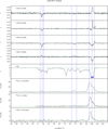 |
Fig. A.2 Same as Fig. A.1, but for G29.957-0.018 |
| In the text | |
|
Fig. A.3 Same as Fig. 2, but for G29.935-0.053. The bottom panel includes an enlarged view of the [C II] 158 µm line for better visibility of the faint emission or absorption components, and/or baseline ripples. |
| In the text | |
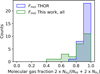 |
Fig. A.4 As Fig. 5, but for Tspin = 50K. |
| In the text | |
|
Fig. A.5 Optical depth of the OH lines at 1612, 1665, 1667 and 1720 MHz, as well of H I toward the seven pixels toward G29.935-0.053 of the upGREAT/SOFIA [12C II] observations, as well as accompanying C18O (2–1) (APEX/PI230) and stacked radio recombination lines (40″, GLOSTAR; Brunthaler et al. 2021; Khan et al. 2024). The maps in the middle panel are repeated for clarity from row 2 in Fig. 7. |
| In the text | |
|
Fig. B.1 [O I] 63 µm emission toward G29.935-0.053. For each spectrum, we show the average of all data (black). We only show the [C II] 158 µm emission for reference in pixel 1, as the other pixels are closer to the central beam than for [C II] 158 µm and do not overlap. Offsets from the source position are indicated in arcsec. |
| In the text | |
|
Fig. B.2 [C II] 158 µm emission toward G31.388-0.383. For each spectrum, we show the average of all data (black), as well as averages by reference position. Note that only vertical polarization (“V”) is available for Pixel 2. The gray-shaded region is masked as it is contaminated by emission in the reference position. |
| In the text | |
|
Fig. B.3 [O I] 63 µm emission toward G31.388-0.383. For each spectrum, we show the average of all data (black). We only show the [C II] 158 µm emission for reference in pixel 1, as the other pixels are closer to the central beam than for [C II] 158 µm and do not overlap. Several pixels show residual low-frequency baseline ripples. The gray-shaded region around 25 km s-1 is masked due to residual artefacts from atmospheric corrections. |
| In the text | |
|
Fig. B.4 [C II] 158 µm emission toward G29.935-0.053. For each spectrum, we show the average of all data (black), as well as averages by reference position. Note that only vertical polarization (“V”) is available for Pixel 2. |
| In the text | |
|
Fig. B.5 Zoom-in on the low-level [C II] 158 µm emission in G29.935-0.053. Colors and spectra as in Fig. B.4. |
| In the text | |
|
Fig. B.6 [C II] 158 µm and [13C II] emission toward G29.935-0.053. Colors and spectra as in Fig. B.4, with the spectra in each subplot shifted to the rest frequency of each line. |
| In the text | |
Current usage metrics show cumulative count of Article Views (full-text article views including HTML views, PDF and ePub downloads, according to the available data) and Abstracts Views on Vision4Press platform.
Data correspond to usage on the plateform after 2015. The current usage metrics is available 48-96 hours after online publication and is updated daily on week days.
Initial download of the metrics may take a while.