| Issue |
A&A
Volume 700, August 2025
|
|
|---|---|---|
| Article Number | A75 | |
| Number of page(s) | 15 | |
| Section | Galactic structure, stellar clusters and populations | |
| DOI | https://doi.org/10.1051/0004-6361/202554349 | |
| Published online | 06 August 2025 | |
A kinematically constrained kick distribution for isolated neutron stars
1
Department of Astrophysics/IMAPP, Radboud University,
PO Box 9010, 6500 GL Nijmegen,
The Netherlands
2
School of Physics and Astronomy, Monash University, Clayton,
Victoria
3800,
Australia
3
The ARC Center of Excellence for Gravitational Wave Discovery – OzGrav,
Australia
4
Department of Physics, University of Warwick,
Coventry
CV4 7AL,
UK
★ Corresponding author: This email address is being protected from spambots. You need JavaScript enabled to view it.
Received:
3
March
2025
Accepted:
1
July
2025
Abstract
Context. The magnitudes of the velocity kicks that neutron stars (NSs) obtain at their formation have long been a topic of discussion, with the latest studies analysing the velocities of young pulsars and favouring a bimodal kick distribution.
Aims. In previous work, a novel method was proposed to determine kicks based on the eccentricity of Galactic trajectories, which is also applicable to older objects. We applied this method to the isolated pulsars with a known parallax – both young and old – in order to kinematically constrain the NS natal kick distribution and investigate its proposed bimodality. Since this method is applicable to older pulsars, we effectively increase the sample size with ~50% compared to the pulsars younger than 10 Myr.
Methods. We assumed the velocity vectors of the pulsars to be distributed isotropically in the local standard of rest frame, and for each pulsar we sampled 100 velocities taking into account this assumption. These velocity vectors were used to trace back the trajectories of the NSs through the Galaxy and estimate their eccentricity. Then, we simulated kicked objects in order to evaluate the relationship between kick magnitude and Galactic eccentricity, which was used to infer the kicks corresponding to the estimated eccentricities.
Results. The resulting kick distributions indeed show a bimodal structure for young pulsars and our fits resemble the ones from literature well. However, for older pulsars the bimodality vanishes and instead we find a log-normal kick distribution peaking at ~200 km/s and a median of ~400 km/s (for velocities below 1000 km/s). We also compare our methods to literature that suggests natal kicks are significantly higher and follow a Maxwellian with σ = 265 km/s. We cannot reproduce these results using their sample and distance estimates, and instead find kicks that are consistent with our proposed distribution.
Conclusions. We conclude that our kinematically constrained kick distribution is well described by a log-normal distribution with μ = 6.38 and σ = 1.01, normalised between 0 and 1000 km/s. This analysis reveals no evidence for bimodality in the larger sample, and we suggest that the bimodality found by existing literature may be caused by their relatively small sample size.
Key words: stars: kinematics and dynamics / stars: neutron / pulsars: general / Galaxy: stellar content
© The Authors 2025
 Open Access article, published by EDP Sciences, under the terms of the Creative Commons Attribution License (https://creativecommons.org/licenses/by/4.0), which permits unrestricted use, distribution, and reproduction in any medium, provided the original work is properly cited.
This article is published in open access under the Subscribe to Open model. This email address is being protected from spambots. You need JavaScript enabled to view it. to support open access publication.
1 Introduction
Neutron stars (NSs) that are observed as isolated pulsars (i.e. pulsars without a binary companion) are known to have relatively high velocities compared to their progenitor stars (e.g. Gunn & Ostriker 1970; Lyne & Lorimer 1994; Lorimer et al. 1997; Cordes & Chernoff 1998), because of which they are thought to have received a (natal) kick at their formation (e.g. Dewey & Cordes 1987; Bailes 1989; Van Paradijs & White 1995; Iben & Tutukov 1996; Fryer & Kalogera 1997; Van den Heuvel & Van Paradijs 1997). These natal kicks are most often associated with anisotropic supernova (SN) explosions (e.g. Janka & Müller 1994; Burrows et al. 1995; Burrows & Hayes 1996; Janka 2017; Gessner & Janka 2018; Müller et al. 2019), although jets launched by the newly formed NS could also potentially play a significant role (e.g. Soker 2010; Bear et al. 2025; Soker 2024; Wang et al. 2024). Moreover, some studies argue that a ‘rocket’ mechanism, caused by anisotropic emission of electromagnetic radiation due to the spin-down of the NS, could provide (minor) contributions to the observed velocities (e.g. Harrison & Tademaru 1975; Lai et al. 2001; Agalianou & Gourgouliatos 2023; Igoshev et al. 2023; Hirai et al. 2024).
Core-collapse SNe cannot only form NSs but also stellarmass black holes, which are therefore potential recipients of natal kicks as well (e.g. Brandt et al. 1995; Nelemans et al. 1999; Jonker & Nelemans 2004; Repetto et al. 2012; Mandel 2016; Andrews & Kalogera 2022; Banagiri et al. 2023; Vigna-Gómez et al. 2024). In addition, when kicked objects are part of a binary, the system also experiences a Blaauw kick through recoil due to mass-loss (Blaauw 1961; Van den Heuvel et al. 2000). This means that the total (systemic) kick imparted on a binary consists of a natal kick and a Blaauw kick for each component that has experienced a SN (e.g. Hills 1983; Tauris et al. 2017; Andrews & Zezas 2019). Determining the magnitude of NS kicks is therefore not only important for studying the Galactic distribution of NSs (e.g. Prokhorov & Postnov 1994; Kiel & Hurley 2009; Ofek 2009; Sartore et al. 2010; Sweeney et al. 2022; Song et al. 2024) but also for the rates and locations of the mergers of compact binaries and the resulting transient signals (e.g. Fryer et al. 1999; Voss & Tauris 2003; Church et al. 2011; Abbott et al. 2017; Vigna-Gómez et al. 2018; Zevin et al. 2020; Iorio et al. 2023; Gaspari et al. 2024a,b; Wagg et al. 2025), as well as important for understanding the SN mechanism (e.g. Nagakura et al. 2019; Müller 2020; Coleman & Burrows 2022; Burrows et al. 2024; Kondratyev et al. 2024; Janka & Kresse 2024) and therefore also the mass distributions of compact objects (e.g. Disberg & Nelemans 2023; Schneider et al. 2023; Laplace et al. 2025).
In an attempt to determine the natal kicks of NSs, several studies have analysed the velocities of (young) pulsars (e.g. Arzoumanian et al. 2002; Brisken et al. 2003a; Hobbs et al. 2005; Faucher-Giguère & Kaspi 2006; Verbunt et al. 2017; Igoshev 2020; Disberg & Mandel 2025, see also Appendix A), often by formulating statistical estimates of the (unknown) radial component of the velocity vector relative to the observer. For example, Hobbs et al. (2005) employed a deconvolution technique (similar to the CLEAN algorithm of Högbom 1974) to infer the full 3D velocity from the observed 1D and 2D pulsar velocities, and argued that the velocity distribution of pulsars younger than 3 Myr approximates the natal kick distribution and is well described by a Maxwellian distribution with σ = 265 km/s. However, Verbunt & Cator (2017) find that (1) there are systematic errors because of which the distance estimates used by Hobbs et al. (2005) that are based on dispersion measures (Cordes & Chernoff 1998; Yao et al. 2017) are likely inaccurate (as confirmed by Deller et al. 2019), and (2) it is difficult to explain the observed transverse 2D velocities of pulsars using the kick distribution of Hobbs et al. (2005).
Because of these concerns, Verbunt et al. (2017) developed a formalism to compare the observed properties of pulsars directly to potential kick distributions, and applied this method to pulsars with distances estimated through parallax instead of dispersion measure. After Deller et al. (2019) significantly expanded the sample of pulsars with parallax estimates, Igoshev (2020) applied the method of Verbunt et al. (2017) to the complete pulsar sample. Both Verbunt et al. (2017) and Igoshev (2020) find that a distribution consisting of two Maxwellians provides a better fit to the data than a single Maxwellian (for details see Appendix A). However, since they compare the proposed distributions directly to observations they stress that this does not necessarily mean that the kick distribution is truly bimodal, it could also mean that the kick distribution is simply wider than a single Maxwellian. After all, for any non-Maxwellian underlying kick distribution adding Maxwellians improves the accuracy of the fit.
There are, however, several reasons why the observed NSs could indeed follow a bimodal kick distribution, the first of which is a dichotomy in the formation mechanism. For example, electron-capture supernovae (ECSNe) (Miyaji et al. 1980; Nomoto 1987; Takahashi et al. 2013; Doherty et al. 2017) from single stars such as super-AGB stars can account for 2-20% of all SNe (Poelarends et al. 2008; Doherty et al. 2015) and are thought to result in smaller natal kicks compared to the canonical corecollapse SNe (Van den Heuvel 2010, and references therein). Small natal kicks could also be the result of interactions in binary stars, which are relevant since the population of isolated NS contains NSs that are born in binaries and have received a kick large enough to unbind the system (although binary disruptions due to mass loss or natal kicks result in different velocities for the escaped pulsar, see e.g. Beniamini & Piran 2024). Mass transfer in a binary can strip the NS progenitor and lead to stripped and ultra-stripped SNe (Podsiadlowski et al. 2004; Tauris et al. 2013, 2015), which in turn result in small natal kicks. However, it has been shown that these smaller kicks would not be sufficient to unbind the binary, and hence that isolated NSs born in binaries can only represent the upper tail of the kick distribution (Kuranov et al. 2009). More recently, SN simulations suggest that there are likely multiple ranges of zero-age main-sequence masses leading to NS formation (e.g. Ertl et al. 2016; Müller et al. 2016; Kresse et al. 2021). In particular, Burrows et al. (2024) find two classes of progenitors: low mass and low compactness that lead to kicks of ~100-200 km/s and high mass and high compactness that lead to kicks of ~300-1000 km/s. These two classes could hypothetically correspond to the two Maxwellians found by Verbunt et al. (2017) and Igoshev (2020).
The methods of Hobbs et al. (2005), Verbunt et al. (2017), and Igoshev (2020) constrain natal kicks by analysing the velocities of young pulsars. This motivation of this choice is that a sample of old pulsars would be biased towards low kick in at least two ways: (1) the Galactic trajectories become more eccentric as a result of the kicks, because of which the objects are more likely to be observed near their Galactic apocentre where they have reduced speeds relative to their initial velocities (Hansen & Phinney 1997; Disberg et al. 2024a), and (2) NSs that receive high kicks migrate outwards more quickly and therefore become less likely to be observed as they age (Cordes 1986; Lyne & Lorimer 1994). In order to eliminate the first of these biases, Disberg et al. (2024b) proposed a method of inferring kicks (i.e. the systemic kicks of binary NSs) based on the shape of their Galactic trajectory, which remains close to circular for low kicks and becomes more eccentric for increasing kick magnitude. This method employs the entire Galactic orbit instead of the presentday circular velocity to infer kicks and should therefore also provide relatively accurate estimates for older NSs. The advantages of such an approach are two-fold. Firstly, the use of older pulsars provides a second, entirely independent sample of NSs on which the kick distribution can be determined while accounting for the evolution of their velocity as they migrate through the Galactic potential. Secondly, the older pulsars expand the sample with measured parallax, making it less prone to noise due to low-number statistics compared to the sample containing only young sample with measured parallax, while retaining the advantage of parallax measurements over (likely more uncertain) distance estimates through dispersion measures.
We applied the method of Disberg et al. (2024b) to the isolated pulsars from the samples of Verbunt et al. (2017) and Igoshev (2020) in order to kinematically constrain the natal kick distribution of NSs and compare it to the results from literature. In Sect. 2, we discuss the distance estimates formulated by Verbunt & Cator (2017) and Verbunt et al. (2017) and analyse the Galactic trajectories of the pulsars. Then, in Sect. 3, we describe and expand the method of Disberg et al. (2024b). The resulting kick distributions are shown in Sect. 4 and are compared to estimates from existing literature. Finally, we summarise our conclusions in Sect. 5.
2 Pulsars
In order to estimate the natal kicks of NSs, we first employed the formalism of Verbunt & Cator (2017, as used by Verbunt et al. 2017 and Igoshev 2020) to determine pulsar distances through their observed parallaxes (Sect. 2.1). Then, we estimated the 3D velocity vectors of these pulsars and computed their Galactic trajectories, which allowed us to investigate their kinematic ages as well as their Galactic eccentricities (Sect. 2.2).
2.1 Distances
Because of systematic uncertainties in distance estimates through dispersion measures, Verbunt et al. (2017) limited their analysis to pulsars with known parallax. In order to infer the distance of a pulsar based on its parallax, Verbunt & Cator (2017) defined the conditional probability of observing a parallax equal to ωobs when the true distance equals D as:
![Mathematical equation: P(\omega_{\text{obs}}\text{\hspace{.4mm}}|\text{\hspace{.4mm}}D)\propto\exp\left(-\dfrac{\left(\left[D/\text{kpc}\right]^{-1}-\left[\omega_{\text{obs}}/\text{mas}\right]\right)^2}{2\left[\sigma_\omega/\text{mas}\right]^2}\right),](/articles/aa/full_html/2025/08/aa54349-25/aa54349-25-eq1.png) (1)
(1)
where σω is the measurement error for the parallax. Then, they defined the prior probability of observing a pulsar with a distance D. If a pulsar is observed at a certain sky location, the distance probability is not uniformly distributed but follows the density of the Galactic pulsar population. For this reason, Verbunt & Cator (2017) employed the prior distance function from Verbiest et al. (2012), which equals (in the notation of Igoshev et al. 2016b):
 (2)
(2)
where z and R are the galactocentric height and cylindrical radius of the pulsar, respectively. These values are related to the distance and the observed sky locations (i.e. the galactic co-ordinates l and b) through:
 (3)
(3)
with R⊙ the galactocentric cylindrical radius of the Sun, which we take to be equal to 8.122 kpc (GRAVITY Collaboration 2018). Since P(ωobs | D) is relatively well constrained due to the accuracy of parallax measurements, the values of the parameters in Eq. (2) do not affect the inferred distances significantly (as shown by Igoshev 2020). The distance to a pulsar is inferred through (cf. Eq. (5) of Verbunt & Cator 2017):
 (4)
(4)
which is a function of D depending on the observed parallax (ωobs) and the sky co-ordinates l and b (through Eq. (3)).
We considered the Verbunt et al. (2017) pulsar sample (based on data from Chatterjee et al. 2001; Brisken et al. 2002, 2003b; Chatterjee et al. 2004, 2009; Deller et al. 2009; Kirsten et al. 2015, taken from the ATNF catalogue1 of Manchester et al. 2005) and the Igoshev (2020) sample (which more than doubles the Verbunt et al. sample by adding data from Deller et al. 2019). This means that the Verbunt et al. sample is a subset of the Igo-shev sample. We computed the probability distribution of their distances through Eq. (4), and for each pulsar we sampled 102 distances from this distribution. These distance estimates were combined with the observed sky locations to determine their galactocentric locations. In Fig. 1 we show the median locations of the pulsars in both samples (where we only show the pulsars in the Igoshev sample that are not in the Verbunt et al. sample). In Appendix B we show the distributions of the pulsar distances, where ~80% of the Verbunt et al. sample and ~60% of the (total) Igoshev sample is located in the solar neighbourhood (which we defined as D ≤ 2 kpc). Moreover, the majority of pulsars are located at x > 0 kpc (cf. Fig. 5 of Chrimes et al. 2021). This is also noted by Igoshev (2020), who suggest this might be due to some regions of the Galaxy being unavailable for very long baseline interferometry (VLBI) measurements.
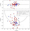 |
Fig. 1 Median locations of the pulsars in the sample of Verbunt et al. (2017, blue dots) and the expansion made by Igoshev (2020, red dots), where the distances are determined through their parallaxes (Eq. (4)). The dashed line shows the solar neighbourhood (i.e. D < 2 kpc) whereas the dotted line shows the solar galactocentric radius (R = 8.122 kpc, GRAVITY Collaboration 2018). |
2.2 Trajectories
Having determined the distances to the pulsars in the Verbunt et al. and the Igoshev samples, we turned to the observed proper motions in order to estimate their velocities. That is, the proper motions can be combined with the distances to obtain the 2D transverse velocity vectors (i.e. vt) which are the projection of the full 3D velocity vector on the sky (and corrected for the transverse component of the Sun’s velocity). However, the radial component of the velocity vector (i.e. vr) cannot be constrained from observations, so in order to estimate the pulsar velocities we follow the method of Gaspari et al. (2024a) in assuming isotropy to determine the probability distribution of vr. They compared two options: isotropy in the galactocentric frame (GC isotropy) and isotropy in the local standard of rest frame (LSR isotropy). However, Disberg et al. (2024b) showed that LSR isotropy is a more accurate assumption (for any given kick magnitude). For this reason we choose LSR isotropy to determine the pulsar velocity vectors. Following this assumption, the radial component of the velocity vector was estimated through:
 (5)
(5)
where vLSR,t and vLSR,r are the transverse and radial components of the LSR velocity, respectively, and θ = arccos u with u being uniformly sampled between −1 and 1. For each sampled pulsar location, we took a uniformly sampled value of u and calculated vr which combined with vt determines the velocity vector.
Having obtained 102 locations and velocities for each pulsars, we flipped the estimated velocity vectors and used GALPY2 v .1.10.0 (Bovy 2015) to trace back the trajectories through the Milky Way using the Galactic potential of McMillan (2017), where we - similarly to Disberg et al. (2024a,b) - set the circular velocity at R⊙ equal to νφ,⊙ = 245.6 km/s (GRAVITY Collaboration 2018). We computed the pulsar trajectories for 1 Gyr and evaluated them every 1 Myr.
The sets of pulsar trajectories allowed us to estimate the kinematic ages (τkin) of the pulsars, which are defined as the time that has passed since their last disc crossing (i.e. at z = 0 kpc). After all, since NSs are formed in SNe of massive stars, which are located in the thin disc at z ≈ 0 kpc, the last disc crossing can provide a lower bound on the age of a NS. The kinematic ages can, then, be compared to the characteristic spin-down ages of the pulsars (τc), which are defined through their rotational period and its derivative (τc = P/(2Ṗ), e.g. Shapiro & Teukolsky 1983). Although in some cases it seems to be inaccurate (e.g. Jiang et al. 2013; Zhang et al. 2022), the characteristic age is usually considered a reasonable estimate of the true pulsar age (as e.g. argued by Maoz & Nakar 2025). Several studies have compared kinematic and characteristic ages (e.g. Lyne et al. 1982; Cordes & Chernoff 1998; Brisken et al. 2003a) and in particular Noutsos et al. (2013) and Igoshev (2019) find a general agreement between the two (independent) age estimates. Here, we compared τkin to τc in order to test whether the assumption of LSR isotropy in the distribution of vr (which influences τkin) is consistent with the assumptions behind τc. In Fig. 2 we show the kinematic age distributions - that follow from the sets of pulsar trajectories - versus the characteristic ages. Indeed, the assumption of LSR isotropy results in the majority of the median kinematic age estimates to differ less than ~20% from the corresponding characteristic ages. There are, however, a few pulsars with τkin exceeding τc substantially, which could either mean that the assumption of LSR isotropy is invalid or that τc is not indicative of the true age (e.g. due to post-SN fallback on the NS, as discussed by Igoshev et al. 2016a). In particular, we considered pulsars where median τkin exceeds τc with more than 5 Myr to have potentially uncertain ages. Nevertheless, in general we deem the characteristic age a reliable age estimate and consistent with the assumption of LSR isotropy.
In order to use the method of Disberg et al. (2024b) to kinematically constrain the natal kick of the pulsars, we first investigated the shape (i.e. eccentricity) of their Galactic trajectories. After all, a larger kick disturbs the initial circular orbits more and therefore results in a more eccentric path through the Galaxy. Since we have established that τc is a reasonable age estimate, we limited our analysis to the pulsar trajectories that do not deviate from the Galactic disc when traced back for a period equal to the characteristic age. That is, we conservatively adopted the constraint that the traced-back trajectories should be positioned within R ≤ 20 kpc and |z| ≤ 1 kpc at t = τc. Although for a few pulsars this decreases the amount of trajectories significantly (i.e. J1321+8323, J1543+0929, J1840+5640, J2046+1540, J2046-0421, J2248-0101, J2346-0609), the median exclusion rate is only 3%. We evaluate the cylindrical radii (i.e. the Galactic distances projected on the Galactic plane) of the selected trajectories and take their minimum and maximum values (Rmin and Rmax, respectively). The eccentricity of the Galactic orbit is then defined as:
 (6)
(6)
analogous to a Keplerian eccentricity (although the trajectories are not Keplerian due to the Galactic potential). If an object that starts in a circular Galactic orbits experiences no kick, then Rmin = Rmax and ẽ ≈ 0. In contrast, if the object receives an extremely large kick, it will escape the Galaxy meaning Rmax >> Rmin and ẽ ≈ 1.
In Fig. 3, we show the resulting eccentricity distributions (cf. Fig. 9 of Disberg et al. 2024b) for four subsets: the ‘young’ pulsars as defined by Igoshev (2020, i.e. τc ≤ 3 Myr) and Verbunt et al. (2017, i.e. τc ≤ 10 Myr), as well as old pulsars (i.e. 40 Myr ≤ τc ≤ 1 Gyr) that have obtained (galactocentric) velocities ~200 km/s (independent of kick distribution, see Appendix B of Disberg et al. 2024a) and pulsars in between these two categories (i.e. 10 Myr ≤ Tc ≤ 40 Myr, see Appendix A of Disberg et al. 2024a). We note that the oldest pulsar in the samples has a characteristic age of τc = 575 Myr, but we set the range of the oldest bin to 1 Gyr for consistency with the simulation introduced in Sect. 3. The eccentricity distributions shown in Fig. 3 peak at ẽ ≈ 1 for the young pulsars. For older pulsars this peak starts to shift to lower eccentricities, in fact the oldest pulsars peak at ẽ ≈ 0. The small eccentricities indicate that if older pulsars were observed to have small velocities, then these cannot be explained by the deceleration due to galactic drift (as discussed by Hansen & Phinney 1997; Disberg et al. 2024a) because this would require eccentric orbits. This means that the shift is likely due to the fact that high kicks displace NSs to relatively large offsets, making them less likely to be observed after a certain amount of time and therefore introducing a selection effect (as discussed by Cordes 1986; Lyne & Lorimer 1994). Besides this general shift to lower values of ẽ, the eccentricity distributions encode the natal NS kicks (see e.g. the peak at ẽ ≈ 0.45 for the oldest pulsars). Lastly, we note that applying the method of Disberg et al. (2024b) to these pulsars will result in more accurate kick estimates for older pulsars (i.e. τc ≳ 10 Myr) compared to methods that only estimate their current velocities (e.g. Hobbs et al. 2005; Verbunt et al. 2017; Igoshev 2020). At the cost of having to consider selection effects (such as NSs that receive large kicks and escape the Galaxy not being observable after a certain amount of time), this method effectively expands the sample of pulsars with relatively accurate kick estimates, making it more robust against noise caused by low-number statistics.
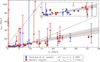 |
Fig. 2 Kinematic ages (τkin) versus characteristic spin-down ages (τc) for the pulsars in the sample of Verbunt et al. (2017, blue) and the expansion of Igoshev (2020, red) with characteristic ages below 40 Myr. The kinematic ages were determined through the sets of pulsar trajectories, where the squares are set at the median values and the whiskers show the 68% ranges. The dotted line depicts τkin = τc and the shaded region shows a 20% error on τc. If the median kinematic age exceeds the characteristic age with more than 5 Myr we show it as a triangle instead of a square, because the question arises whether these pulsars affect the accuracy of resulting kick distributions. |
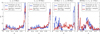 |
Fig. 3 Galactic eccentricities for the pulsars in the samples of Verbunt et al. (2017, blue) and Igoshev (2020, red), as defined in Eq. (6). The distributions are shown in histograms with bins of 0.01, and divided in four ranges of τc consisting of N pulsars. |
3 Method
Having evaluated the eccentricities of the pulsars’ trajectories, we employed the method of Disberg et al. (2024b) to estimate their kicks. In order to do this, we expanded their simulation which determines the relationship between Galactic eccentricity and kick magnitude (Sect. 3.1). Then, we discussed how we inferred kicks based on the simulation and the eccentricity estimates (Sect. 3.2).
3.1 Simulation
In order to relate the estimated eccentricities to kicks, we simulated populations of objects receiving kicks with different magnitudes and analysed the eccentricities of the resulting orbits. For each simulation, we seeded 103 objects in a Gaussian annulus at z = 0 kpc, described by:
 (7)
(7)
Faucher-Giguère & Kaspi (2006) first proposed this distribution for pulsars, which was fitted by Sartore et al. (2010) to the pulsar distribution of Yusifov & Küçük (2004) resulting in Rd = 7.04 kpc and σd = 1.83 kpc. We note that a completely different initial distribution (i.e. an exponential disc) likely results in similar kick estimates (Disberg et al. 2024b). Having obtained the initial positions of the objects, we gave them a circular (azimuthal) velocity as determined by the Galactic potential of McMillan (2017), and added an isotropically sampled kick velocity with a magnitude vkick. Based on the initial positions and velocities, we computed the Galactic trajectories of the sampled objects for 1 Gyr (using GALPY of Bovy 2015), after which each object was assigned an eccentricity through Eq. (6). In order to track the population that is in the solar neighbourhood (i.e. D ≤ 2 kpc) at any given time, we initialised the orbit of the Sun (using the results of Reid & Brunthaler 2004; Drimmel & Poggio 2018; GRAVITY Collaboration 2018; Bennett & Bovy 2019, see also Eqs. (3) and (4) of Disberg et al. 2024a) and selected objects that are within 2 kpc at a given time. After all, it is not that for an individual object its value of ẽ changes over time, but the population of objects that is located in the solar neighbourhood does. We then repeated the simulation for different values of vkick with intervals of 10 km/s up to 1000 km/s (corresponding to the kick ranges found by Burrows et al. 2024), obtaining time-dependent relationships between vkick and ẽ for the solar neighbourhood population.
In Fig. 4 we show the resulting vkick versus ẽ distributions (cf. Fig. 10 of Disberg et al. 2024b), for time intervals corresponding to the τc ranges in Fig. 3. For all time intervals there is a close relationship between kick and eccentricity for vkick ≲ 400 km/s, meaning our method is most sensitive in this region. For higher kicks the objects pile up just below 1, since they are likely to escape the Galaxy. After all, while the true Galactic eccentricity equals 1 for escaping objects, the estimated value of ẽ is limited by the integration time of the simulation. Moreover, Disberg et al. (2024b) distinguish between objects that follow the rotational direction of the Sun (i.e. ‘prograde’ orbits) and objects that travel against the direction of the Solar System (i.e. ‘retrograde’ orbits), and these two kinds of orbits can also be found in Fig, 4. That is, for vkick ≲ vLSR (Rd) all objects are prograde since the kick is likely smaller than the initial circular velocity of the object. At higher kicks it becomes possible to receive a kick larger than the initial velocity but in opposite direction, resulting in a retrograde orbit. This peaks at vkick ≈ 2 · vLSR(Rd), which can result in a circular (i.e. ẽ = 0) retrograde orbit (for a more elaborate discussion see Disberg et al. 2024b).
Also, Fig. 4 shows how over time the contribution of high kicks to the solar neighbourhood population decreases. This supports our previous statement on the small eccentricities of Galactic pulsars, namely that they are caused by the selection effect proposed by Cordes (1986) and Lyne & Lorimer (1994) by which highly kicked pulsars disappear from the solar neighbourhood over time. This selection effect causes a peak at ẽ ≈ 1, which over time shifts to a peak at ẽ ≈ 0 (for a uniform kick distribution), similarly to the observed pulsar eccentricities shown in Fig. 3. Lastly, for older pulsars the ρe density displays an oscillation at low ẽ, this is not physical but a consequence of the ẽ peak shifting significantly between subsequent kick bins at vkick ≲ 30 km/s.
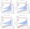 |
Fig. 4 Distributions of vkick versus ẽ for objects in the solar neighbourhood (D ≤ 2 kpc) as resulting from the simulations, shown in 2D histograms on a logarithmic colour scale with eccentricity bins of 0.01 and velocity bins of 10 km/s. We show the eccentricities found in four time-bins, corresponding to the bins from Fig. 3. Each distribution also shows the integrated ẽ and vkick densities (ρe and ρv, respectively). The dotted black lines show one and two times the circular velocity at Rd = 7.04 kpc (from Eq. (7)). For the distribution of the total population see Appendix C. |
3.2 Inference
We have estimated the eccentricities of the observed pulsars (Fig. 3) and investigated the relationship between eccentricity and kick magnitude (Fig. 4), and we used this to infer the kicks corresponding to the observed eccentricities. That is, the simulations provide insight into the amount of eccentric orbits given a certain kick magnitude but we are interested in inferring the kick magnitude given a certain eccentricity. In order to do this we employed Bayes’ theorem, for which the prior distributions of the eccentricities and kicks are needed (see also Appendix B of Disberg et al. 2024b). First, we divided the simulations in time bins corresponding to the ranges shown in Figs. 3 and 4, and separated prograde from retrograde orbits (where we note that ~90% of the observed pulsar trajectories are prograde). For a value of ẽ from the estimated distributions shown in Fig. 3, we compare it with simulated results that are in the same time bin as the corresponding τc and orbit the Galaxy in the same rotational direction. Then, the prior probability of observing an eccentricity ẽ is proportional to the amount of simulated orbits with this eccentricity: P(ẽ) ∝ N(ẽ). Likewise, the prior probability of observing an object that received a kick equal to vkick is given by P(vkick) ∝ N(vkick). Also, the probability of observing a value of ẽ given a certain vkick is the amount of eccentricities in the corresponding bin normalised for objects that have received this kick: P(ẽ | vkick) ∝ N(ẽ | vkick)/N(vkick). In other words, this conditional probability is proportional to the value of a cell in Fig. 4 when each row is normalised individually. The defined probabilities can then be inserted into Bayes’ theorem, which gives:
 (8)
(8)
That is, the probability that a kick of magnitude vkick is the cause of an observed (either prograde or retrograde) orbit with an eccentricity ẽ is given by the value of a cell in Fig. 4 where the columns are normalised individually.
However, for the most eccentric orbits the normalisation is not straightforward, because the corresponding kick distribution starts to shift to vkick > 1000 km/s and this region is not included in the simulations. For this reason, we normalise these distributions as if the amount of orbits per ẽ bin does not decrease, extrapolating the preceding trend with d log10(N)/dẽ = 17. In the top panel of Fig. 5 we show this correction in the amounts of objects per eccentricity bin considered for the normalisation. In the bottom panel of the figure we show how the kick distributions per ẽ (normalised using this correction) shift to higher kick magnitudes. Without the correction these renormalised distributions would cause unnecessary noise in the kick estimates.
For each individual pulsar there is not one single value of ẽ but a distribution of eccentricities (i.e. Dẽ) which defines the probability density of ẽ (i.e. P(ẽ | Dẽ)). The sum of these distributions were shown in Fig. 3 (for certain ranges of τc). The individual kick distributions as constrained through the eccentricity estimates (i.e. P(vkick | Dẽ)) are then determined by weighting the inferred kick per ẽ as given by Eq. (8) by the eccentricity distributions and integrating over ẽ, or:
 (9)
(9)
Moreover, when combining the kick estimates of individual pulsars to show the total kick distributions (of pulsars with a certain age), we divide the results by the prior P(vkick) in order to account for the fact that the contribution of highly kicked objects decreases for older pulsars (because of which an old pulsar with a high kick should have an increased weight). We note that this correction (as well as the correction from Fig. 5) has no noticeable effect on the results of Disberg et al. (2024b).
The method described in this section makes several assumptions in its kick estimation. For example, we assumed that pulsar formation takes place in the Galactic disc at z = 0 kpc, where the initial velocity of the pulsar consists of a perfectly circular Galactic orbit and an isotropic natal kick. Moreover, the relationships shown in Fig. 4 are produced by integrating our simulation over several time intervals, but the distribution of pulsar ages within these intervals is not uniform. We also do not consider a possible binary origin in which the natal kicks unbind the binary and thus lose a fraction of their initial kinetic energy (e.g. Bailes 1989; Kalogera 1996; Tauris & Takens 1998; Kuranov et al. 2009). However, Chrimes et al. (2023) find that the velocities of unbound NSs are dominated by the natal kicks, and Kapil et al. (2023) also conclude that a binary origin has no significant effect on their simulated kicks. Renzo et al. (2019), in turn, find that only ~1% of disrupted massive stars (i.e. potential NS progenitors) obtain velocities above 30 km/s, whereas ejected helium stars can obtain higher velocities but are significantly rarer. The hypothetical effects of a ‘rocket’ mechanism are neglected as well (cf. Hirai et al. 2024). Moreover, Spitzer & Schwarzschild (1951, 1953) discuss the effect of overdensities in the Galactic disc (such as giant molecular clouds) on stellar velocities (see also e.g. Dehnen & Binney 1998; Sellwood & Binney 2002), and Madau & Blaes (1994) argue that this dynamical heating should apply to (old) NSs as well. However, Ofek (2009) argues that dynamical heating becomes important for velocities below (τc · 328 km2 s−2 Gyr−1)1/2, meaning that for an old pulsar with τc = 1 Gyr it is relevant when the velocity is less than ~20 km/s, and he therefore concludes this effect can be neglected due to the relatively high velocities of NSs. Another potential effect assumed to be negligible is the alignment of kick and NS spin (e.g. Johnston et al. 2005; Biryukov & Beskin 2024) because of which the observed pulsar velocities are not isotropic and the kicks of young pulsars might be overestimated by ~15% (Mandel & Igoshev 2023). These assumptions add uncertainty to the kick estimates that follow from this method, although we note that most of them apply to the method of Verbunt et al. (2017) and Igoshev (2020) as well.
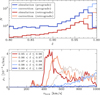 |
Fig. 5 Correction made to the normalisation of the simulated vkick versus ẽ distributions of young objects (the figure shows the example of τc ≤ 10 Myr). The top panel shows the amount of objects per eccentricity bin for progrades (blue) and retrogrades (red) orbits, as well as the corrected amounts used for the normalisation (lightblue and lightred, respectively). The bottom panel shows the kick distributions for the five ẽ bins closest to 1 (indicated by colour), normalised using the corrected values shown above. |
4 Kicks
Having estimated the eccentricities of the pulsars in the Verbunt et al. and Igoshev samples, we used the method of Disberg et al. (2024b) - as described above - to infer the natal kicks of these pulsars. We show and discuss the resulting kick distributions for both samples and for different ranges of Tc (Sect. 4.1) and compare them to kinematically constrained estimates using the pulsar sample of Hobbs et al. (2005) as well as distributions established in literature (Sect. 4.2).
4.1 Results
We applied the method discussed in Sect. 3 to the eccentricity estimates shown in Sect. 2, for the Verbunt et al. sample and the expanded Igoshev sample. We determined the results for these complete samples as well as the subsets shown in Fig. 3 (i.e. τc ≤ 3 Myr, τc ≤ 10 Myr, 10 Myr < τc ≤ 40 Myr, and 40 Myr < τc ≤ 1 Gyr). In Fig. 6 we show our resulting kick distributions for the pulsar samples, and fit multiple distributions to the results. That is, similarly to Disberg et al. (2024b) we fit log-normal distributions:
 (10)
(10)
where the fitted parameters are listed in Table 1. Moreover, similarly to Verbunt et al. (2017) and Igoshev (2020) we fit Maxwellians to our results (i.e. the results for the complete samples and their ‘young’ subsets):
 (11)
(11)
They find, however, that NS kicks are better described by a distribution that combines two Maxwellians. We therefore also fit a double-Maxwellian to our results, defined as:
 (12)
(12)
where σ1 < σ2 and the parameter w determines the fraction of NS kicks situated in the lower Maxwellian component. The distributions of our results as well as the fitted distributions are normalised between 0 km/s and 1000 km/s. The fitted parameters of the Maxwellians and double-Maxwellians are listed in Table 2 and compared to the parameters from the corresponding literature.
The first two rows in Fig. 6 respectively show the estimated kick distributions for pulsars younger than 3 Myr (similar to Hobbs et al. 2005; Igoshev 2020) and younger than 10 Myr (similar to Verbunt et al. 2017). When we fit (double-)Maxwellians to the results corresponding to the ‘young’ subsets of the Verbunt et al. and the Igoshev samples, we find that the resulting distributions resemble the corresponding fits of Verbunt et al. (2017) and Igoshev (2020) remarkably well. We thus find that our kick distributions for the young pulsars in their samples agree with their results. The single Maxwellian fits, however, are clearly not representative of the underlying kick distribution, because of which a comparison with, for instance, the Maxwellian found by Hobbs et al. (2005) is not meaningful. The double-Maxwellian fits, in contrast, are an accurate description of the results. However, although the kicks of the τc ≤ 3 Myr pulsars in the Igoshev sample show a clear bimodality, the kicks of the corresponding τc ≤ 10 Myr pulsars in the Verbunt et al. sample are less bimodal than the double-Maxwellian fit suggests. This might be due to our method not being sensitive enough to resolve the bimodal structure, but since Verbunt et al. (2017) determine their fits through a direct comparison with observed data there is no way to examine whether they actually do find a clearly bimodal structure. Nevertheless, our results do suggest a bimodality for the τc ≤ 3 Myr pulsars in the Igoshev sample, and are compatible with bimodality in the τc ≤ 10 Myr pulsars in the Verbunt et al. sample.
However, the τc ≤ 10 Myr pulsars in the Igoshev sample do not show a bimodal structure at all (in fact, the kicks agree well with the log-normal fit). This set of pulsars contains the ‘young’ subsets of both the Verbunt et al. and the Igoshev samples, so if the bimodality of those double-Maxwellian fits were physical then one would expect the τc ≤ 10 Myr pulsars in the Igoshev sample to also follow a bimodal distribution. These results, though, show a single peak at vkick ≈ 200 km/s at the same place where the τc ≤ 3 Myr subset shows a dearth of pulsars. This is difficult to explain if the true natal kick distribution for NSs follows a bimodal distribution similar to the one found by Igoshev (2020). Indeed, in the subsequent age ranges the older pulsars in the Igoshev sample also follow an approximately log-normal distribution peaking at vkick ≈ 200 km/s. The corresponding distributions for the Verbunt et al. sample only contain 4 and 5 pulsars, respectively, because of which it is difficult to draw strong conclusions from these results. For the oldest pulsars the correction of dividing by the prior kick probabilities causes unnecessary noise at vkick > 600 km/s, which is why we exclude this region from the fits and normalisations.
In the bottom row of Fig. 6 we show the kick distributions for the complete samples (i.e. the sum of the separate distributions weighted by the amount of pulsars). Our results for the complete Verbunt et al. sample differ slightly from the fit made by Verbunt et al. (2017). This is likely due to the fact that we find that this sample contains relatively high kicks for pulsars older than 10 Myr, and Disberg et al. (2024a) show that - up to a certain point - higher kicks result in lower observed velocities for older pulsars. Therefore the older pulsars probably contribute to the lower Maxwellian peak of Verbunt et al. (2017), while we find that this is actually an underestimation of their actual kick. Our results for the complete Verbunt et al. sample do, however, match the results for the complete Igoshev sample better. In fact, the fit made by Igoshev (2020) also aligns with our results (and is less bimodal than the double-Maxwellian structure might suggest). This agreement is probably coincidental, since the (kickindependent) velocity distribution of older pulsars found by Disberg et al. (2024a) might be aligning with the natal kick distribution (peaking at ~200 km/s). Nevertheless, we argue that (1) the kinematically constrained pulsar kick distributions are consistent with a single peak at 200 km/s, and (2) the resulting kick distribution for the complete Igoshev sample appears to describe the distributions for the different age-selected samples relatively well and approximately follows a log-normal distribution.
The question arises whether the bimodality in the young pulsar kicks is consistent with the log-normal distributions that older pulsars appear to follow. Considering that (relatively) young pulsars remain the least biased with regard to kick velocities, we adopted the log-normal fit to the Igoshev sample for τc ≤ 10 Myr (i.e. μ = 6.38 and σ = 1.01) as the fiducial NS natal kick distribution determined through kinematic constraints. Furthermore, we employed a one-sample Kolmogorov-Smirnov (KS) test in order to evaluate the hypothesis that the underlying natal kick distribution for the results in the different age ranges equals the fiducial log-normal distribution. Relevantly, in Fig. 7 we show the cumulative distribution functions (CDFs) of the young and complete samples as examples. We computed the KS statistic for the results shown in the panels of Fig. 6, and find that for no distribution it exceeds the critical value (as listed by Massey 1951) above which we can reject the hypothesis at a 0.05 level of significance (although for τc > 40 Myr the difference becomes relatively small). We therefore conjecture that -despite the fact that Valli et al. (2025) predict that unbound NSs indeed form a second peak at ~100 km/s - this bimodality may be caused by noise due to low-number statistics (cf. the analysis of the observed binary black hole mass distribution of Farah et al. 2023 and Adamcewicz et al. 2024). Moreover, one might suspect that there are pulsars in the young samples that are older than their τc might suggest. We therefore investigated the results for the young samples where we excluded the pulsars with a τkin that exceeds τc by more than 5 Myr (as marked in Fig. 2). In Appendix D we show that these results still include the bimodality, meaning it is probably not caused by pulsars of which τkin and τc do not align.
Parameters of the log-normal distributions (Eq. (10)) fitted to the results shown in Fig. 6, for the pulsar samples of Verbunt et al. (2017) and Igoshev (2020).
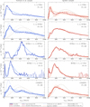 |
Fig. 6 Resulting kick estimates (solid blue and red lines) for the pulsars in the sample of Verbunt et al. (2017, blue and left column) and the expanded sample of Igoshev (2020, red and right column) after applying the method described in Sect. 3 to the eccentricity estimates shown in Fig. 3. The samples - consisting of N pulsars - are divided in four age ranges (i.e. τc ≤ 3 Myr, τc ≤ 10 Myr, 10 Myr < τc ≤ 40 Myr, 40 Myr < τc ≤ 1 Gyr, and the complete sample) as shown in the different rows. We fitted log-normal distributions (solid light blue/red) to the results in each panel (listed in Table 1), and to the results corresponding to the ages analysed in the literature we also fitted Maxwellians and double-Maxwellians (dashed light blue/red and grey lines, listed in Table 2). The corresponding distributions posed by Verbunt et al. (2017) and Igoshev (2020) are also shown (dotted light blue/red and grey lines). For ages 40 Myr < τc ≤ 1 Gyr we excluded the results for vkick > 600 km/s (dotted blue/red lines) in the normalisation and fits. We adopted the log-normal fit to the results for the τc ≤ 10 Myr Igoshev sample as the fiducial natal NS kick distribution. |
Parameters of the (double-)Maxwellians fitted to our results for the Verbunt et al. (2017) and Igoshev (2020) samples (fit), compared to the results from the corresponding literature (lit.), for young pulsars and the complete samples.
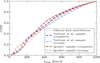 |
Fig. 7 Cumulative distributions of the fiducial kick distribution (lognormal with μ = 6.00 and σ = 0.85, grey) compared to the kick distributions from Verbunt et al. (2017, blue) and Igoshev (2020, red), for their complete samples as well as young subsets (blue/red and light blue/red, respectively). The distributions are all normalised in the region of 0 km/s ≤ vkick ≤ 1000 km/s. |
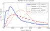 |
Fig. 8 Kinematically constrained kick distributions for the young pulsars using the pulsar sample - including distance estimates - of Hobbs et al. (2005), considering the age ranges of τc ≤ 3 Myr (blue solid line, with a sample size N = 46) and τc ≤ 10 Myr (dotted light blue line, N = 83). The dashed grey line shows a Maxwellian fit to the τc < 3 Myr results (resulting in σ = 159(5) km/s). For comparison we also show the fit of Hobbs et al. (2005, dashed light red line, a Maxwellian with σ = 265 km/s) and the fiducial kick distribution based on the results for the pulsars with parallax estimates (dashed red line). |
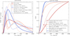 |
Fig. 9 Comparison between our fiducial kick distribution (red solid line) and kick distributions as found in existing literature. In the left panel the comparison is made with probability density functions (PDFs) from existing literature on NS natal kicks (i.e. Arzoumanian et al. 2002; Brisken et al. 2003a; Faucher-Giguère & Kaspi 2006; Verbunt et al. 2017; Igoshev 2020; Igoshev et al. 2021; Disberg & Mandel 2025, omitting the erroneous distribution of Hobbs et al. 2005), while in the right panel we compare our natal kicks and the results of Disberg & Mandel (2025) to CDFs of the systemic kicks of binaries that include compact objects (i.e. Atri et al. 2019; O’Doherty et al. 2023; Zhao et al. 2023; Disberg et al. 2024b, where the modes are displayed as dots). The shown distributions are all normalised between 0 km/s and 1000 km/s, and their parameters are listed in Appendix A. |
4.2 Comparisons
The fiducial kick distribution and the distributions found by Verbunt et al. (2017) and Igoshev (2020) contain lower kick velocities than the commonly used kick distribution of Hobbs et al. (2005, i.e. a Maxwellian with σ = 265 km/s). This difference could hypothetically be caused by the fact that the Hobbs et al. sample is not limited to pulsars with observed parallaxes but mainly uses distance estimates through dispersion measures. In order to test this, we applied our method to the Hobbs et al. sample - using their distance estimates - and compared it to the parallax samples from Fig. 6. In Fig. 8 we show the results for the pulsars in the Hobbs et al. sample that are either younger than 3 Myr (for comparison with Hobbs et al. 2005; Igoshev 2020) or 10 Myr (for comparison with Verbunt et al. 2017). Both of these age ranges result in a kick distribution showing one clear peak at −100−200 km/s.
The figure shows how our results differ significantly from the Maxwellian found by Hobbs et al. (2005), which peaks at −400 km/s. In Fig. 6, the single-Maxwellian fits peak at these high kick velocities as well, but (1) this is coincidental since Hobbs et al. (2005) show that their results follow their fit well (in contrast to the single Maxwellians in Fig. 6), and (2) the Maxwellian fit in Fig. 8 differs significantly. More importantly, our results for the Hobbs et al. sample are more similar to our results for the parallax samples, and seem relatively well described by our fiducial kick distribution. The latter includes slightly higher kicks, though, but this is similar to the difference between the Verbunt et al. sample and the Igoshev sample. In fact, we note that the results for the young pulsars in the Hobbs et al. sample (Fig. 8) are especially similar to the results for the young pulsars in the Verbunt et al. sample (Fig. 6). We therefore argue that it may be difficult to explain the difference between the results of these studies through inaccuracy in distance estimates. After all, we were able to use our method to recreate the results of Verbunt et al. (2017) and Igoshev (2020), but failed to reproduce the results of Hobbs et al. (2005) even though we used their distance estimates. Lastly, we note the similarity between our kick estimates (in particular the results for the young pulsars in the Hobbs et al. and Verbunt et al. samples) and the theoretical -probabilistic - kick prescription of Mandel & Müller (2020, see also Mandel et al. 2021 and Kapil et al. 2023).
While this article was in review, Disberg & Mandel (2025) analysed the present-day velocities of young pulsars in order to obtain a kick velocity distribution (and applied the method described in this paper to pulsars older than 10 Myr, finding consistent results). Their resulting kick distribution is in general similar to our fiducial kick distribution: it is a log-normal distribution peaking at −200 km/s. The main difference between these two distributions is that they predict a smaller contribution of the high-velocity tail. After all, as stated before, our method is mainly sensitive to velocities ≤ 400 km/s. Moreover, Disberg & Mandel (2025) show that the Maxwellian distribution found by Hobbs et al. (2005) is based on an erroneous histogram interpretation that misses a Jacobian to correct for its logarithmic bin sizes. Correcting for the missing Jacobian indeed results in kicks similar to our results shown in Fig. 8, explaining why we are unable to reproduce the Maxwellian distribution of Hobbs et al. (2005) and solving the tension in the literature caused by their work.
In the left panel of Fig. 9 we compare our fiducial kick distribution to results from literature (i.e. Arzoumanian et al. 2002; Brisken et al. 2003a; Faucher-Giguère & Kaspi 2006; Verbunt et al. 2017; Igoshev 2020; Igoshev et al. 2021; Disberg & Mandel 2025). The figure shows that existing literature on NS kicks indeed tend to find distributions that peak around ~100-200 km/s. Since we omit the distribution of Hobbs et al. (2005), the literature paints a relatively consistent picture. In the right panel of Fig. 9 we also show the results of studies estimating the systemic kicks of binaries that include a NS or black hole (i.e. Atri et al. 2019; O’Doherty et al. 2023; Zhao et al. 2023; Disberg et al. 2024b). The natal kicks of isolated NSs peak at kick velocities a factor ~2 higher than the systemic kicks of these binaries. There are at least two reasons for this: (1) high natal kicks can unbind a binary, hence the observed binaries that experienced a SN kick are biased towards low kicks (e.g. Beniamini & Piran 2016), and (2) the natal kick contributes to the systemic kick with a weight equal to the NS mass over the binary mass, and therefore the systemic kicks is usually smaller when the natal kick dominates over the Blaauw kick. In order to investigate these two effects it would be interesting to attempt to reconcile the observed natal and systemic kick distributions, for example through a population synthesis.
5 Conclusions
In this work, we have analysed the pulsars in the samples of Verbunt et al. (2017) and Igoshev (2020), and estimated the eccentricities of their Galactic orbits (Sect. 2). Moreover, we expanded the simulation of Disberg et al. (2024b) which determines the relationship between kick magnitude and Galactic eccentricity (Sect. 3). The results of this simulation were combined with the eccentricity estimates in order to determine the natal kicks of the pulsars in the Verbunt et al. and Igoshev samples (Sect. 4). Based on our analysis we come to the following conclusions:
For most young pulsars in the Verbunt et al. and Igoshev samples (Fig. 1), their kinematic age and characteristic age align relatively well (Fig. 2). This means that LSR isotropy is compatible with the characteristic age estimates, which provides confidence in both assumptions.
The younger pulsars follow more eccentric Galactic orbits (Eq. (6) and Fig. 3), which is likely due to the selection effect of older pulsars with high kicks reaching relatively large offsets, making them less likely to be observed. The simulated orbits (Fig. 4) follow this trend as well, and display a close relationship between kick magnitude and Galactic eccentricity (at least for vkick ≲ 400km/s). After correcting the normalisation for the most eccentric orbits (Fig. 5), we used this relationship to infer the kick velocities of the pulsars.
The resulting kinematically constrained kick distributions, which were divided in different age bins (Fig. 6), are consistent with NS natal kicks following a log-normal distribution with μ = 6.38 and σ = 1.01 - normalised between 0 and 1000 km/s - which peaks at ~200 km/s and has a median of ~400 km/s (Fig. 7). In particular, double-Maxwellians (Eq. (12)) fitted to the results for young pulsars resemble the results of Verbunt et al. (2017, for τc ≤ 10 Myr) and Igoshev (2020, for τc < 3 Myr). However, we argue that the bimodality found for young pulsar kicks might not be physical but instead caused by noise due to low-number statistics.
If we apply our method to the pulsar sample - including distance estimates - of Hobbs et al. (2005), the results do not resemble their Maxwellian fit (Fig. 8). Instead, our results do not show a significant difference between the kicks of the pulsars in the Hobbs et al. sample and ones in the Verbunt et al. sample. This can be explained by the fact that Disberg & Mandel (2025) show that the Maxwellian distribution of Hobbs et al. (2005) is based on an erroneous histogram interpretation that misses a Jacobian. Neglecting their Maxwellian, the existing literature on NS kicks paints a relatively consistent picture with distributions peaking at ~100-200 km/s (Fig. 9).
In general, we also note that Disberg et al. (2024b) show that their method gives results very similar to the method of Atri et al. (2019, who trace back trajectories and analyse peculiar velocities at disc crossings), while we show that this method also gives results similar to the method of Verbunt et al. (2017). Because of this we can be relatively confident in these methods.
Our fiducial log-normal kick distribution has median and mean values of ~400 km/s and ~600 km/s, respectively. This is, for example, compatible with the constraint posed by Popov et al. (2000) that the average NS kick should exceed ~200-300 km/s. Willcox et al. (2021), in turn, estimate that in their sample 5±2% of isolated NS kick velocities are below 50 km/s, and they show that in their model this is compatible with observations of binary NSs and NSs in globular clusters (since these have escape velocities on this scale, see e.g. Katz 1975; Sigurdsson & Phinney 1995). However, our log-normal fit predicts <1% of kicks to be below this limit, which might be in tension with their model. Nevertheless, in the kinematically constrained kick estimates for the complete Igoshev sample (Fig. 6), ~3% of kicks are below 50 km/s, which agrees with the findings of Willcox et al. (2021) and might indicate that our log-normal fit might be insufficient in describing the low end of the kick distribution in detail (e.g. in the context of NS populations in globular clusters). These kind of details and further applications of the NS natal kick distribution could provide an interesting basis for future research.
Acknowledgements
The authors are thankful to the referee for helpful comments that helped improve this paper, and thank Ilya Mandel for useful discussions. P.D. acknowledges support from the Australian Research Council Centre of Excellence for Gravitational Wave Discovery (OzGrav) through project number CE230100016. N.G. acknowledges studentship support from the Dutch Research Council (NWO) under the project number 680.92.18.02, and A.J.L. was supported by the European Research Council (ERC) under the European Union’s Horizon 2020 research and innovation programme (grant agreement No. 725246). In this work, we made use of NUMPY (Harris et al. 2020), SCIPY (Virtanen et al. 2020), MATPLOTLIB (Hunter 2007), GALPY (Bovy 2015), and ASTROPY, a community-developed core Python package and an ecosystem of tools and resources for astronomy (Astropy Collaboration 2013, 2018, 2022).
Appendix A Kick distributions
In Fig. 9 we display various distributions, of which the parameters are listed in Table A.1. For instance, Arzoumanian et al. (2002) define a two-component Gaussian:
![Mathematical equation: \rho_{2\text{G}}(v\text{\hspace{.4mm}}|\text{\hspace{.4mm}}\sigma_1,\sigma_2,w)=4\pi v^2\left[w\,\rho_{\text{G}}(v\text{\hspace{.4mm}}|\text{\hspace{.4mm}}\sigma_1)+(1-w)\,\rho_{\text{G}}(v\text{\hspace{.4mm}}|\text{\hspace{.4mm}}\sigma_2)\right],](/articles/aa/full_html/2025/08/aa54349-25/aa54349-25-eq13.png) (A.1)
(A.1)
using the Gaussian-like function:
 (A.2)
(A.2)
Moreover, O’Doherty et al. (2023) employ a beta distribution:
 (A.3)
(A.3)
where Γ denotes the gamma function and s is a scaling factor above which the function is set to zero.
Appendix B Pulsar distances
The distributions of the distances between the Solar System and the pulsars in the samples of Verbunt et al. (2017) and Igoshev (2020) are shown in Fig. B.1 (for their Galactocentric locations, see Fig. 1). We note that for ≳50% of pulsars D ≤ 2 kpc.
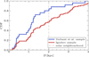 |
Fig. B.1 Cumulative distributions of the pulsar distances corresponding to the samples of Verbunt et al. (2017, blue) and Igoshev (2020, red), together with the edge of the solar neighbourhood (dashed grey line). |
Appendix C Total population
In Fig. 4 we show the relationship between kick magnitude and eccentricity for objects that are at a certain time in the solar neighbourhood. In Fig. C.1, we also show the (time-independent) distribution for the total population, which aligns relatively well with the results for the solar neighbourhood.
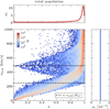 |
Fig. C.1 Distributions of vkick versus ẽ for the total population as resulting from the simulations (similarly to Fig. 4). The distribution also shows the integrated ẽ and vkick densities (ρe and ρv, respectively). The dotted black lines show one and two times the circular velocity at Rd = 7.04 kpc (from Eq. 7). |
Appendix D Kinematic age selection
In order to investigate whether the pulsars with τkin > τc + 5 Myr (as marked in Fig. 2) cause the bimodality in the young pulsar sample (as shown in Fig. 6), we determined the kick distributions for the young samples while excluding these pulsars. In Fig. D.1 we show the kick distributions of young pulsars with aligning τc and τkin. In these kick distributions the bimodality is still present, meaning it is unlikely caused by the pulsars with inconsistent age estimates.
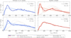 |
Fig. D.1 Resulting kick estimates (blue and red solid lines) for the young pulsars in the sample of Verbunt et al. (2017, blue and left column) and the expanded sample of Igoshev (2020, red and right column), similar to Fig. 6 but excluded pulsars with τkin > τc + 5 Myr. We fitted log-normal distributions (solid light blue/red) to the results in each panel, and to the results corresponding to the ages analysed by the literature we also fitted Maxwellians and double-Maxwellians (dashed light blue/red and grey lines). The corresponding distributions posed by Verbunt et al. (2017) and Igoshev (2020) are also shown (dotted light blue/red and grey lines). |
Appendix E Igoshev sample
The two pulsar samples used in the main analysis of this paper are the samples of Verbunt et al. (2017) and Igoshev (2020), where the Igoshev sample expands the Verbunt et al. sample with the results of Deller et al. (2019). The question arises whether the pulsars that were added to the Verbunt et al. sample to form the Igoshev sample follow a kick distribution similar to the results of Verbunt et al. (2017). In Fig. D.1 we compare the kinemati- cally constrained kick distributions of the Verbunt et al. sample to the kick distributions for the pulsars that are only present in the Igoshev sample. The resulting distributions do not describe a consistent kick distribution: the Verbunt et al. kicks peak at −100 km/s, whereas the expansion of the Igoshev sample has a dearth at ~100 km/s and peaks at ~50 km/s and ~300—400 km/s. This could either be caused by low-number statistics or perhaps an observation bias in the observations of Deller et al. (2019).
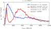 |
Fig. E.1 Kinematically constrained kick distributions for the sample of Verbunt et al. (2017, blue line) and the sample of pulsars that are only in the Igoshev (2020, red line) sample (i.e. the observations of Deller et al. 2019), for τc ≤ 3 Myr. The dotted lines show the kick distributions posed by Verbunt et al. (2017) and Igoshev (2020), where we note that the former is based on pulsars with τc ≤ 10 Myr instead of τc ≤ 3 Myr. |
References
- Abbott, B. P., Abbott, R., Abbott, T. D., et al. 2017, ApJ, 850, L40 [NASA ADS] [CrossRef] [Google Scholar]
- Adamcewicz, C., Lasky, P. D., Thrane, E., & Mandel, I. 2024, ApJ, 975, 253 [Google Scholar]
- Agalianou, V., & Gourgouliatos, K. N. 2023, MNRAS, 522, 5879 [NASA ADS] [CrossRef] [Google Scholar]
- Andrews, J. J., & Zezas, A. 2019, MNRAS, 486, 3213 [NASA ADS] [CrossRef] [Google Scholar]
- Andrews, J. J., & Kalogera, V. 2022, ApJ, 930, 159 [NASA ADS] [CrossRef] [Google Scholar]
- Arzoumanian, Z., Chernoff, D. F., & Cordes, J. M. 2002, ApJ, 568, 289 [NASA ADS] [CrossRef] [Google Scholar]
- Astropy Collaboration (Robitaille, T. P., et al.) 2013, A&A, 558, A33 [NASA ADS] [CrossRef] [EDP Sciences] [Google Scholar]
- Astropy Collaboration (Price-Whelan, A. M., et al.) 2018, AJ, 156, 123 [Google Scholar]
- Astropy Collaboration (Price-Whelan, A. M., et al.) 2022, ApJ, 935, 167 [NASA ADS] [CrossRef] [Google Scholar]
- Atri, P., Miller-Jones, J. C. A., Bahramian, A., et al. 2019, MNRAS, 489, 3116 [NASA ADS] [CrossRef] [Google Scholar]
- Bailes, M. 1989, ApJ, 342, 917 [Google Scholar]
- Banagiri, S., Doctor, Z., Kalogera, V., Kimball, C., & Andrews, J. J. 2023, ApJ, 959, 106 [NASA ADS] [CrossRef] [Google Scholar]
- Bear, E., Shishkin, D., & Soker, N. 2025, Res. Astron. Astrophys., 25, 045008 [Google Scholar]
- Beniamini, P., & Piran, T. 2016, MNRAS, 456, 4089 [NASA ADS] [CrossRef] [Google Scholar]
- Beniamini, P., & Piran, T. 2024, ApJ, 966, 17 [NASA ADS] [CrossRef] [Google Scholar]
- Bennett, M., & Bovy, J. 2019, MNRAS, 482, 1417 [NASA ADS] [CrossRef] [Google Scholar]
- Biryukov, A., & Beskin, G. 2024, arXiv e-prints [arXiv:2412.12017] [Google Scholar]
- Blaauw, A. 1961, Bull. Astron. Inst. Netherlands, 15, 265 [NASA ADS] [Google Scholar]
- Bovy, J. 2015, ApJS, 216, 29 [NASA ADS] [CrossRef] [Google Scholar]
- Brandt, W. N., Podsiadlowski, P., & Sigurdsson, S. 1995, MNRAS, 277, L35 [NASA ADS] [Google Scholar]
- Brisken, W. F., Benson, J. M., Goss, W. M., & Thorsett, S. E. 2002, ApJ, 571, 906 [NASA ADS] [CrossRef] [Google Scholar]
- Brisken, W. F., Fruchter, A. S., Goss, W. M., Herrnstein, R. M., & Thorsett, S. E. 2003a, AJ, 126, 3090 [NASA ADS] [CrossRef] [Google Scholar]
- Brisken, W. F., Thorsett, S. E., Golden, A., & Goss, W. M. 2003b, ApJ, 593, L89 [NASA ADS] [CrossRef] [Google Scholar]
- Burrows, A., & Hayes, J. 1996, Phys. Rev. Lett., 76, 352 [Google Scholar]
- Burrows, A., Hayes, J., & Fryxell, B. A. 1995, ApJ, 450, 830 [NASA ADS] [CrossRef] [Google Scholar]
- Burrows, A., Wang, T., Vartanyan, D., & Coleman, M. S. B. 2024, ApJ, 963, 63 [NASA ADS] [CrossRef] [Google Scholar]
- Chatterjee, S., Cordes, J. M., Lazio, T. J. W., et al. 2001, ApJ, 550, 287 [Google Scholar]
- Chatterjee, S., Cordes, J. M., Vlemmings, W. H. T., et al. 2004, ApJ, 604, 339 [NASA ADS] [CrossRef] [Google Scholar]
- Chatterjee, S., Brisken, W. F., Vlemmings, W. H. T., et al. 2009, ApJ, 698, 250 [NASA ADS] [CrossRef] [Google Scholar]
- Chrimes, A. A., Levan, A. J., Groot, P. J., Lyman, J. D., & Nelemans, G. 2021, MNRAS, 508, 1929 [NASA ADS] [CrossRef] [Google Scholar]
- Chrimes, A. A., Levan, A. J., Eldridge, J. J., et al. 2023, MNRAS, 522, 2029 [Google Scholar]
- Church, R. P., Levan, A. J., Davies, M. B., & Tanvir, N. 2011, MNRAS, 413, 2004 [NASA ADS] [CrossRef] [Google Scholar]
- Coleman, M. S. B., & Burrows, A. 2022, MNRAS, 517, 3938 [NASA ADS] [CrossRef] [Google Scholar]
- Cordes, J. M. 1986, ApJ, 311, 183 [NASA ADS] [CrossRef] [Google Scholar]
- Cordes, J. M., & Chernoff, D. F. 1998, ApJ, 505, 315 [NASA ADS] [CrossRef] [Google Scholar]
- Dehnen, W., & Binney, J. J. 1998, MNRAS, 298, 387 [NASA ADS] [CrossRef] [Google Scholar]
- Deller, A. T., Tingay, S. J., Bailes, M., & Reynolds, J. E. 2009, ApJ, 701, 1243 [NASA ADS] [CrossRef] [Google Scholar]
- Deller, A. T., Goss, W. M., Brisken, W. F., et al. 2019, ApJ, 875, 100 [NASA ADS] [CrossRef] [Google Scholar]
- Dewey, R. J., & Cordes, J. M. 1987, ApJ, 321, 780 [NASA ADS] [CrossRef] [Google Scholar]
- Disberg, P., & Mandel, I. 2025, arXiv e-prints [arXiv:2505.22102] [Google Scholar]
- Disberg, P., & Nelemans, G. 2023, A&A, 676, A31 [NASA ADS] [CrossRef] [EDP Sciences] [Google Scholar]
- Disberg, P., Gaspari, N., & Levan, A. J. 2024a, A&A, 687, A272 [NASA ADS] [CrossRef] [EDP Sciences] [Google Scholar]
- Disberg, P., Gaspari, N., & Levan, A. J. 2024b, A&A, 689, A348 [NASA ADS] [CrossRef] [EDP Sciences] [Google Scholar]
- Doherty, C. L., Gil-Pons, P., Siess, L., Lattanzio, J. C., & Lau, H. H. B. 2015, MNRAS, 446, 2599 [Google Scholar]
- Doherty, C. L., Gil-Pons, P., Siess, L., & Lattanzio, J. C. 2017, PASA, 34, e056 [NASA ADS] [CrossRef] [Google Scholar]
- Drimmel, R., & Poggio, E. 2018, RNAAS, 2, 210 [NASA ADS] [Google Scholar]
- Ertl, T., Janka, H. T., Woosley, S. E., Sukhbold, T., & Ugliano, M. 2016, ApJ, 818, 124 [NASA ADS] [CrossRef] [Google Scholar]
- Farah, A. M., Edelman, B., Zevin, M., et al. 2023, ApJ, 955, 107 [NASA ADS] [CrossRef] [Google Scholar]
- Faucher-Giguère, C.-A., & Kaspi, V. M. 2006, ApJ, 643, 332 [CrossRef] [Google Scholar]
- Fryer, C., & Kalogera, V. 1997, ApJ, 489, 244 [NASA ADS] [CrossRef] [Google Scholar]
- Fryer, C. L., Woosley, S. E., & Hartmann, D. H. 1999, ApJ, 526, 152 [NASA ADS] [CrossRef] [Google Scholar]
- Gaspari, N., Levan, A. J., Chrimes, A. A., & Nelemans, G. 2024a, MNRAS, 527, 1101 [Google Scholar]
- Gaspari, N., Stevance, H. F., Levan, A. J., Chrimes, A. A., & Lyman, J. D. 2024b, A&A, 692, A21 [NASA ADS] [CrossRef] [EDP Sciences] [Google Scholar]
- Gessner, A., & Janka, H.-T. 2018, ApJ, 865, 61 [Google Scholar]
- GRAVITY Collaboration (Abuter, R., et al.) 2018, A&A, 615, L15 [NASA ADS] [CrossRef] [EDP Sciences] [Google Scholar]
- Gunn, J. E., & Ostriker, J. P. 1970, ApJ, 160, 979 [NASA ADS] [CrossRef] [Google Scholar]
- Hansen, B. M. S., & Phinney, E. S. 1997, MNRAS, 291, 569 [NASA ADS] [Google Scholar]
- Harris, C. R., Millman, K. J., Van der Walt, S. J., et al. 2020, Nature, 585, 357 [NASA ADS] [CrossRef] [Google Scholar]
- Harrison, E. R., & Tademaru, E. 1975, ApJ, 201, 447 [NASA ADS] [CrossRef] [Google Scholar]
- Hills, J. G. 1983, ApJ, 267, 322 [NASA ADS] [CrossRef] [Google Scholar]
- Hirai, R., Podsiadlowski, P., Heger, A., & Nagakura, H. 2024, ApJ, 972, L18 [Google Scholar]
- Hobbs, G., Lorimer, D. R., Lyne, A. G., & Kramer, M. 2005, MNRAS, 360, 974 [Google Scholar]
- Högbom, J. A. 1974, A&AS, 15, 417 [Google Scholar]
- Hunter, J. D. 2007, Comput. Sci. Eng., 9, 90 [NASA ADS] [CrossRef] [Google Scholar]
- Iben, Icko, J., & Tutukov, A. V. 1996, ApJ, 456, 738 [NASA ADS] [CrossRef] [Google Scholar]
- Igoshev, A. P. 2019, MNRAS, 482, 3415 [Google Scholar]
- Igoshev, A. P. 2020, MNRAS, 494, 3663 [NASA ADS] [CrossRef] [Google Scholar]
- Igoshev, A. P., Elfritz, J. G., & Popov, S. B. 2016a, MNRAS, 462, 3689 [Google Scholar]
- Igoshev, A. P., Verbunt, F., & Cator, E. 2016b, A&A, 591, A123 [NASA ADS] [CrossRef] [EDP Sciences] [Google Scholar]
- Igoshev, A. P., Chruslinska, M., Dorozsmai, A., & Toonen, S. 2021, MNRAS, 508, 3345 [NASA ADS] [CrossRef] [Google Scholar]
- Igoshev, A. P., Hollerbach, R., & Wood, T. 2023, MNRAS, 525, 3354 [Google Scholar]
- Iorio, G., Mapelli, M., Costa, G., et al. 2023, MNRAS, 524, 426 [NASA ADS] [CrossRef] [Google Scholar]
- Janka, H.-T. 2017, ApJ, 837, 84 [Google Scholar]
- Janka, H.-T., & Kresse, D. 2024, Ap&SS, 369, 80 [NASA ADS] [CrossRef] [Google Scholar]
- Janka, H. T., & Müller, E. 1994, A&A, 290, 496 [Google Scholar]
- Jiang, L., Zhang, C.-M., Tanni, A., & Zhao, H.-H. 2013, Int. J. Mod. Phys. Conf. Ser., 23, 95 [NASA ADS] [CrossRef] [Google Scholar]
- Johnston, S., Hobbs, G., Vigeland, S., et al. 2005, MNRAS, 364, 1397 [NASA ADS] [CrossRef] [Google Scholar]
- Jonker, P. G., & Nelemans, G. 2004, MNRAS, 354, 355 [Google Scholar]
- Kalogera, V. 1996, ApJ, 471, 352 [Google Scholar]
- Kapil, V., Mandel, I., Berti, E., & Müller, B. 2023, MNRAS, 519, 5893 [NASA ADS] [CrossRef] [Google Scholar]
- Katz, J. I. 1975, Nature, 253, 698 [NASA ADS] [CrossRef] [Google Scholar]
- Kiel, P. D., & Hurley, J. R. 2009, MNRAS, 395, 2326 [NASA ADS] [CrossRef] [Google Scholar]
- Kirsten, F., Vlemmings, W., Campbell, R. M., Kramer, M., & Chatterjee, S. 2015, A&A, 577, A111 [NASA ADS] [CrossRef] [EDP Sciences] [Google Scholar]
- Kondratyev, I. A., Moiseenko, S. G., & Bisnovatyi-Kogan, G. S. 2024, Phys. Rev. D, 110, 083025 [Google Scholar]
- Kresse, D., Ertl, T., & Janka, H.-T. 2021, ApJ, 909, 169 [NASA ADS] [CrossRef] [Google Scholar]
- Kuranov, A. G., Popov, S. B., & Postnov, K. A. 2009, MNRAS, 395, 2087 [Google Scholar]
- Lai, D., Chernoff, D. F., & Cordes, J. M. 2001, ApJ, 549, 1111 [NASA ADS] [CrossRef] [Google Scholar]
- Laplace, E., Schneider, F. R. N., & Podsiadlowski, P. 2025, A&A, 695, A71 [NASA ADS] [CrossRef] [EDP Sciences] [Google Scholar]
- Lorimer, D. R., Bailes, M., & Harrison, P. A. 1997, MNRAS, 289, 592 [NASA ADS] [Google Scholar]
- Lyne, A. G., & Lorimer, D. R. 1994, Nature, 369, 127 [NASA ADS] [CrossRef] [Google Scholar]
- Lyne, A. G., Anderson, B., & Salter, M. J. 1982, MNRAS, 201, 503 [Google Scholar]
- Madau, P., & Blaes, O. 1994, ApJ, 423, 748 [Google Scholar]
- Manchester, R. N., Hobbs, G. B., Teoh, A., & Hobbs, M. 2005, AJ, 129, 1993 [Google Scholar]
- Mandel, I. 2016, MNRAS, 456, 578 [Google Scholar]
- Mandel, I., & Igoshev, A. P. 2023, ApJ, 944, 153 [NASA ADS] [CrossRef] [Google Scholar]
- Mandel, I., & Müller, B. 2020, MNRAS, 499, 3214 [NASA ADS] [CrossRef] [Google Scholar]
- Mandel, I., Müller, B., Riley, J., et al. 2021, MNRAS, 500, 1380 [Google Scholar]
- Maoz, D., & Nakar, E. 2025, ApJ, 982, 179 [Google Scholar]
- Massey, F. J. 1951, J. Am. Statist. Assoc., 46, 68 [CrossRef] [Google Scholar]
- McMillan, P. J. 2017, MNRAS, 465, 76 [NASA ADS] [CrossRef] [Google Scholar]
- Miyaji, S., Nomoto, K., Yokoi, K., & Sugimoto, D. 1980, PASJ, 32, 303 [Google Scholar]
- Müller, B. 2020, Liv. Rev. Computat. Astrophys., 6, 3 [Google Scholar]
- Müller, B., Heger, A., Liptai, D., & Cameron, J. B. 2016, MNRAS, 460, 742 [Google Scholar]
- Müller, B., Tauris, T. M., Heger, A., et al. 2019, MNRAS, 484, 3307 [Google Scholar]
- Nagakura, H., Sumiyoshi, K., & Yamada, S. 2019, ApJ, 880, L28 [Google Scholar]
- Nelemans, G., Tauris, T. M., & Van den Heuvel, E. P. J. 1999, A&A, 352, L87 [NASA ADS] [Google Scholar]
- Nomoto, K. 1987, ApJ, 322, 206 [NASA ADS] [CrossRef] [Google Scholar]
- Noutsos, A., Schnitzeler, D. H. F. M., Keane, E. F., Kramer, M., & Johnston, S. 2013, MNRAS, 430, 2281 [NASA ADS] [CrossRef] [Google Scholar]
- O’Doherty, T. N., Bahramian, A., Miller-Jones, J. C. A., et al. 2023, MNRAS, 521, 2504 [CrossRef] [Google Scholar]
- Ofek, E. O. 2009, PASP, 121, 814 [NASA ADS] [CrossRef] [Google Scholar]
- Podsiadlowski, P., Langer, N., Poelarends, A. J. T., et al. 2004, ApJ, 612, 1044 [NASA ADS] [CrossRef] [Google Scholar]
- Poelarends, A. J. T., Herwig, F., Langer, N., & Heger, A. 2008, ApJ, 675, 614 [Google Scholar]
- Popov, S. B., Colpi, M., Treves, A., et al. 2000, ApJ, 530, 896 [NASA ADS] [CrossRef] [Google Scholar]
- Prokhorov, M. E., & Postnov, K. A. 1994, A&A, 286, 437 [Google Scholar]
- Reid, M. J., & Brunthaler, A. 2004, ApJ, 616, 872 [Google Scholar]
- Renzo, M., Zapartas, E., De Mink, S. E., et al. 2019, A&A, 624, A66 [NASA ADS] [CrossRef] [EDP Sciences] [Google Scholar]
- Repetto, S., Davies, M. B., & Sigurdsson, S. 2012, MNRAS, 425, 2799 [Google Scholar]
- Sartore, N., Ripamonti, E., Treves, A., & Turolla, R. 2010, A&A, 510, A23 [NASA ADS] [CrossRef] [EDP Sciences] [Google Scholar]
- Schneider, F. R. N., Podsiadlowski, P., & Laplace, E. 2023, ApJ, 950, L9 [NASA ADS] [CrossRef] [Google Scholar]
- Sellwood, J. A., & Binney, J. J. 2002, MNRAS, 336, 785 [Google Scholar]
- Shapiro, S. L., & Teukolsky, S. A. 1983, Black Holes, White Dwarfs and Neutron Stars: The Physics of Compact Objects (Wiley-VCH) [Google Scholar]
- Sigurdsson, S., & Phinney, E. S. 1995, ApJS, 99, 609 [NASA ADS] [CrossRef] [Google Scholar]
- Soker, N. 2010, MNRAS, 401, 2793 [NASA ADS] [CrossRef] [Google Scholar]
- Soker, N. 2024, arXiv e-prints [arXiv:2409.13657] [Google Scholar]
- Song, Y., Stevenson, S., & Chattopadhyay, D. 2024, arXiv e-prints [arXiv:2406.11428] [Google Scholar]
- Spitzer, Lyman, J., & Schwarzschild, M. 1951, ApJ, 114, 385 [NASA ADS] [CrossRef] [Google Scholar]
- Spitzer, Lyman, J., & Schwarzschild, M. 1953, ApJ, 118, 106 [NASA ADS] [CrossRef] [Google Scholar]
- Sweeney, D., Tuthill, P., Sharma, S., & Hirai, R. 2022, MNRAS, 516, 4971 [NASA ADS] [CrossRef] [Google Scholar]
- Takahashi, K., Yoshida, T., & Umeda, H. 2013, ApJ, 771, 28 [NASA ADS] [CrossRef] [Google Scholar]
- Tauris, T. M., & Takens, R. J. 1998, A&A, 330, 1047 [NASA ADS] [Google Scholar]
- Tauris, T. M., Langer, N., Moriya, T. J., et al. 2013, ApJ, 778, L23 [NASA ADS] [CrossRef] [Google Scholar]
- Tauris, T. M., Langer, N., & Podsiadlowski, P. 2015, MNRAS, 451, 2123 [NASA ADS] [CrossRef] [Google Scholar]
- Tauris, T. M., Kramer, M., Freire, P. C. C., et al. 2017, ApJ, 846, 170 [Google Scholar]
- Valli, R., De Mink, S. E., Justham, S., et al. 2025, [arXiv:2505.08857] [Google Scholar]
- Van den Heuvel, E. P. J. 2010, New A Rev., 54, 140 [Google Scholar]
- Van den Heuvel, E. P. J., & Van Paradijs, J. 1997, ApJ, 483, 399 [CrossRef] [Google Scholar]
- Van den Heuvel, E. P. J., Portegies Zwart, S. F., Bhattacharya, D., & Kaper, L. 2000, A&A, 364, 563 [NASA ADS] [Google Scholar]
- Van Paradijs, J., & White, N. 1995, ApJ, 447, L33 [NASA ADS] [CrossRef] [Google Scholar]
- Verbiest, J. P. W., Weisberg, J. M., Chael, A. A., Lee, K. J., & Lorimer, D. R. 2012, ApJ, 755, 39 [NASA ADS] [CrossRef] [Google Scholar]
- Verbunt, F., & Cator, E. 2017, J. Astrophys. Astron., 38, 40 [Google Scholar]
- Verbunt, F., Igoshev, A., & Cator, E. 2017, A&A, 608, A57 [NASA ADS] [CrossRef] [EDP Sciences] [Google Scholar]
- Vigna-Gómez, A., Neijssel, C. J., Stevenson, S., et al. 2018, MNRAS, 481, 4009 [Google Scholar]
- Vigna-Gómez, A., Willcox, R., Tamborra, I., et al. 2024, Phys. Rev. Lett., 132, 191403 [CrossRef] [Google Scholar]
- Virtanen, P., Gommers, R., Oliphant, T. E., et al. 2020, Nat. Methods, 17, 261 [Google Scholar]
- Voss, R., & Tauris, T. M. 2003, MNRAS, 342, 1169 [Google Scholar]
- Wagg, T., Breivik, K., Renzo, M., & Price-Whelan, A. M. 2025, ApJS, 276, 16 [Google Scholar]
- Wang, N. Y. N., Shishkin, D., & Soker, N. 2024, ApJ, 969, 163 [Google Scholar]
- Willcox, R., Mandel, I., Thrane, E., et al. 2021, ApJ, 920, L37 [NASA ADS] [CrossRef] [Google Scholar]
- Yao, J. M., Manchester, R. N., & Wang, N. 2017, ApJ, 835, 29 [NASA ADS] [CrossRef] [Google Scholar]
- Yusifov, I., & Küçük, I. 2004, A&A, 422, 545 [NASA ADS] [CrossRef] [EDP Sciences] [Google Scholar]
- Zevin, M., Kelley, L. Z., Nugent, A., et al. 2020, ApJ, 904, 190 [NASA ADS] [CrossRef] [Google Scholar]
- Zhang, C.-M., Cui, X.-H., Li, D., et al. 2022, Universe, 8, 628 [NASA ADS] [CrossRef] [Google Scholar]
- Zhao, Y., Gandhi, P., Dashwood Brown, C., et al. 2023, MNRAS, 525, 1498 [NASA ADS] [CrossRef] [Google Scholar]
All Tables
Parameters of the log-normal distributions (Eq. (10)) fitted to the results shown in Fig. 6, for the pulsar samples of Verbunt et al. (2017) and Igoshev (2020).
Parameters of the (double-)Maxwellians fitted to our results for the Verbunt et al. (2017) and Igoshev (2020) samples (fit), compared to the results from the corresponding literature (lit.), for young pulsars and the complete samples.
All Figures
|
Fig. 1 Median locations of the pulsars in the sample of Verbunt et al. (2017, blue dots) and the expansion made by Igoshev (2020, red dots), where the distances are determined through their parallaxes (Eq. (4)). The dashed line shows the solar neighbourhood (i.e. D < 2 kpc) whereas the dotted line shows the solar galactocentric radius (R = 8.122 kpc, GRAVITY Collaboration 2018). |
| In the text | |
|
Fig. 2 Kinematic ages (τkin) versus characteristic spin-down ages (τc) for the pulsars in the sample of Verbunt et al. (2017, blue) and the expansion of Igoshev (2020, red) with characteristic ages below 40 Myr. The kinematic ages were determined through the sets of pulsar trajectories, where the squares are set at the median values and the whiskers show the 68% ranges. The dotted line depicts τkin = τc and the shaded region shows a 20% error on τc. If the median kinematic age exceeds the characteristic age with more than 5 Myr we show it as a triangle instead of a square, because the question arises whether these pulsars affect the accuracy of resulting kick distributions. |
| In the text | |
|
Fig. 3 Galactic eccentricities for the pulsars in the samples of Verbunt et al. (2017, blue) and Igoshev (2020, red), as defined in Eq. (6). The distributions are shown in histograms with bins of 0.01, and divided in four ranges of τc consisting of N pulsars. |
| In the text | |
|
Fig. 4 Distributions of vkick versus ẽ for objects in the solar neighbourhood (D ≤ 2 kpc) as resulting from the simulations, shown in 2D histograms on a logarithmic colour scale with eccentricity bins of 0.01 and velocity bins of 10 km/s. We show the eccentricities found in four time-bins, corresponding to the bins from Fig. 3. Each distribution also shows the integrated ẽ and vkick densities (ρe and ρv, respectively). The dotted black lines show one and two times the circular velocity at Rd = 7.04 kpc (from Eq. (7)). For the distribution of the total population see Appendix C. |
| In the text | |
|
Fig. 5 Correction made to the normalisation of the simulated vkick versus ẽ distributions of young objects (the figure shows the example of τc ≤ 10 Myr). The top panel shows the amount of objects per eccentricity bin for progrades (blue) and retrogrades (red) orbits, as well as the corrected amounts used for the normalisation (lightblue and lightred, respectively). The bottom panel shows the kick distributions for the five ẽ bins closest to 1 (indicated by colour), normalised using the corrected values shown above. |
| In the text | |
|
Fig. 6 Resulting kick estimates (solid blue and red lines) for the pulsars in the sample of Verbunt et al. (2017, blue and left column) and the expanded sample of Igoshev (2020, red and right column) after applying the method described in Sect. 3 to the eccentricity estimates shown in Fig. 3. The samples - consisting of N pulsars - are divided in four age ranges (i.e. τc ≤ 3 Myr, τc ≤ 10 Myr, 10 Myr < τc ≤ 40 Myr, 40 Myr < τc ≤ 1 Gyr, and the complete sample) as shown in the different rows. We fitted log-normal distributions (solid light blue/red) to the results in each panel (listed in Table 1), and to the results corresponding to the ages analysed in the literature we also fitted Maxwellians and double-Maxwellians (dashed light blue/red and grey lines, listed in Table 2). The corresponding distributions posed by Verbunt et al. (2017) and Igoshev (2020) are also shown (dotted light blue/red and grey lines). For ages 40 Myr < τc ≤ 1 Gyr we excluded the results for vkick > 600 km/s (dotted blue/red lines) in the normalisation and fits. We adopted the log-normal fit to the results for the τc ≤ 10 Myr Igoshev sample as the fiducial natal NS kick distribution. |
| In the text | |
|
Fig. 7 Cumulative distributions of the fiducial kick distribution (lognormal with μ = 6.00 and σ = 0.85, grey) compared to the kick distributions from Verbunt et al. (2017, blue) and Igoshev (2020, red), for their complete samples as well as young subsets (blue/red and light blue/red, respectively). The distributions are all normalised in the region of 0 km/s ≤ vkick ≤ 1000 km/s. |
| In the text | |
|
Fig. 8 Kinematically constrained kick distributions for the young pulsars using the pulsar sample - including distance estimates - of Hobbs et al. (2005), considering the age ranges of τc ≤ 3 Myr (blue solid line, with a sample size N = 46) and τc ≤ 10 Myr (dotted light blue line, N = 83). The dashed grey line shows a Maxwellian fit to the τc < 3 Myr results (resulting in σ = 159(5) km/s). For comparison we also show the fit of Hobbs et al. (2005, dashed light red line, a Maxwellian with σ = 265 km/s) and the fiducial kick distribution based on the results for the pulsars with parallax estimates (dashed red line). |
| In the text | |
|
Fig. 9 Comparison between our fiducial kick distribution (red solid line) and kick distributions as found in existing literature. In the left panel the comparison is made with probability density functions (PDFs) from existing literature on NS natal kicks (i.e. Arzoumanian et al. 2002; Brisken et al. 2003a; Faucher-Giguère & Kaspi 2006; Verbunt et al. 2017; Igoshev 2020; Igoshev et al. 2021; Disberg & Mandel 2025, omitting the erroneous distribution of Hobbs et al. 2005), while in the right panel we compare our natal kicks and the results of Disberg & Mandel (2025) to CDFs of the systemic kicks of binaries that include compact objects (i.e. Atri et al. 2019; O’Doherty et al. 2023; Zhao et al. 2023; Disberg et al. 2024b, where the modes are displayed as dots). The shown distributions are all normalised between 0 km/s and 1000 km/s, and their parameters are listed in Appendix A. |
| In the text | |
|
Fig. B.1 Cumulative distributions of the pulsar distances corresponding to the samples of Verbunt et al. (2017, blue) and Igoshev (2020, red), together with the edge of the solar neighbourhood (dashed grey line). |
| In the text | |
|
Fig. C.1 Distributions of vkick versus ẽ for the total population as resulting from the simulations (similarly to Fig. 4). The distribution also shows the integrated ẽ and vkick densities (ρe and ρv, respectively). The dotted black lines show one and two times the circular velocity at Rd = 7.04 kpc (from Eq. 7). |
| In the text | |
|
Fig. D.1 Resulting kick estimates (blue and red solid lines) for the young pulsars in the sample of Verbunt et al. (2017, blue and left column) and the expanded sample of Igoshev (2020, red and right column), similar to Fig. 6 but excluded pulsars with τkin > τc + 5 Myr. We fitted log-normal distributions (solid light blue/red) to the results in each panel, and to the results corresponding to the ages analysed by the literature we also fitted Maxwellians and double-Maxwellians (dashed light blue/red and grey lines). The corresponding distributions posed by Verbunt et al. (2017) and Igoshev (2020) are also shown (dotted light blue/red and grey lines). |
| In the text | |
|
Fig. E.1 Kinematically constrained kick distributions for the sample of Verbunt et al. (2017, blue line) and the sample of pulsars that are only in the Igoshev (2020, red line) sample (i.e. the observations of Deller et al. 2019), for τc ≤ 3 Myr. The dotted lines show the kick distributions posed by Verbunt et al. (2017) and Igoshev (2020), where we note that the former is based on pulsars with τc ≤ 10 Myr instead of τc ≤ 3 Myr. |
| In the text | |
Current usage metrics show cumulative count of Article Views (full-text article views including HTML views, PDF and ePub downloads, according to the available data) and Abstracts Views on Vision4Press platform.
Data correspond to usage on the plateform after 2015. The current usage metrics is available 48-96 hours after online publication and is updated daily on week days.
Initial download of the metrics may take a while.