| Issue |
A&A
Volume 700, August 2025
|
|
|---|---|---|
| Article Number | A190 | |
| Number of page(s) | 23 | |
| Section | Planets, planetary systems, and small bodies | |
| DOI | https://doi.org/10.1051/0004-6361/202554401 | |
| Published online | 19 August 2025 | |
DBNets2.0: Simulation-based inference for planet-induced dust substructures in protoplanetary discs
1
Università degli Studi di Milano, Dipartimento di Fisica,
via Celoria 16,
20133
Milano,
Italy
2
Center for Computational Astrophysics, Flatiron Institute,
162 Fifth Avenue,
New York,
NY 10010,
USA
3
Department of Physics and Astronomy, Stony Brook University,
Stony Brook,
NY 11794,
USA
★ Corresponding author: This email address is being protected from spambots. You need JavaScript enabled to view it.
Received:
6
March
2025
Accepted:
10
June
2025
Abstract
Dust substructures observed in protoplanetary discs can be interpreted as signatures of embedded young planets, whose detection and characterisation would provide a better understanding of planet formation. Traditional techniques used to link the morphology of these substructures to the properties of putative embedded planets present several limitations, which the use of deep learning methods has partly overcome. In our previous work, we used these new techniques to develop DBNets, a tool that uses an ensemble of convolutional neural networks (CNNs) to estimate the mass of putative planets in disc dust substructures. This inference problem, however, is degenerate, as planets of different masses could produce the same rings and gaps if other physical disc properties differ. In this paper, we address this issue by improving our tool to estimate three other disc properties in addition to the planet mass: the disc α-viscosity, the disc scale height, and the dust Stokes number. For a given dust continuum observation, the full joint posterior for these four properties is inferred, exposing the existing degeneracies and enabling the integration of external constraints to improve the planet mass estimates. In addition to this new feature, we also addressed a few minor issues with our previous tool, which reduced its accuracy depending on the resolution of the observations, or in the case of peculiar disc morphologies. The new pipeline involves a CNN that summarises the input images into a set of summary statistics, followed by an ensemble of normalising flows that model the inferred posterior for the target properties. We tested our pipeline on a dedicated set of synthetic observations, using the TARP test and standard metrics to demonstrate that our estimates are good approximations of the actual posteriors. Additionally, we applied the results obtained on the test set to study the presence and shape of degeneracies between pairs of parameters. Finally, we applied the developed pipeline to a set of 49 gaps in 34 protoplanetary disc continuum observations. The results show typically low values of α-viscosity, disc scale heights, and planet masses, with 83% of them being lower than 1 MJ. These low masses are consistent with the non-detections of these putative planets in direct imaging surveys. Our tool is publicly available.
Key words: methods: data analysis / protoplanetary disks / planet / disk interactions
© The Authors 2025
 Open Access article, published by EDP Sciences, under the terms of the Creative Commons Attribution License (https://creativecommons.org/licenses/by/4.0), which permits unrestricted use, distribution, and reproduction in any medium, provided the original work is properly cited.
This article is published in open access under the Subscribe to Open model. This email address is being protected from spambots. You need JavaScript enabled to view it. to support open access publication.
1 Introduction
Continuum observations of dust emission in protoplanetary discs often reveal annular substructures in the form of gaps and rings (e.g. Isella et al. 2016; Andrews et al. 2018; van Terwisga et al. 2018; Huang et al. 2020b). Although other mechanisms have been proposed (e.g. Hawley 2001; Barge et al. 2017; Dullemond & Penzlin 2018; Hu et al. 2019; Bae et al. 2023), a promising explanation for their origin is the presence of embedded planets that gravitationally interact with the disc material (Dipierro et al. 2015; Rosotti et al. 2016; Zhang et al. 2018). In the specific case of the PDS70 transition disc, two planets in the disc cavity have been detected via observations of accretion tracers (Wagner et al. 2018; Haffert et al. 2019; Zhou et al. 2021), direct imaging in the infrared (Keppler et al. 2019; Christiaens et al. 2019; Mesa et al. 2019), and, for PDS70c, in the millimetre and submillimetre (Isella et al. 2019; Benisty et al. 2021). Furthermore, evidence has been presented for candidate planets in other systems with dust substructures, including AS209 (Fedele et al. 2023), AB Aur (Currie et al. 2022), and HD 169142 (Hammond et al. 2023). However, apart from these cases, systematic infrared surveys of discs with substructure have so far had limited success in directly detecting planets, being only able to put upper limits on the mass and temperature of putative embedded planets (e.g. Reggiani et al. 2016; Nielsen et al. 2019; Vigan et al. 2021; Asensio-Torres et al. 2021).
In the planet-disc interaction scenario, the morphology of observed substructures is determined by the physical properties of the planet and the surrounding disc, and it can be used to estimate these quantities. The collation and systematic analysis of substructures thus constitutes a useful tool for studying the population of young planets (Lodato et al. 2019; Zhang et al. 2018), which is difficult to probe with the more standard techniques used for exoplanet detection (e.g. transit, radial velocity). Additionally, it can support observational surveys by testing the consistency of (non-)detections and by identifying promising candidates for new observations.
Several studies have investigated the dependence of substructure morphology on disc and planet properties (e.g. Rosotti et al. 2016; Kanagawa et al. 2016; Dipierro & Laibe 2017), proposing empirical relations that link morphological features, such as gap widths and depths, with the mass of the putative planet and, for example, the disc α-viscosity and scale height. Nevertheless, these formulae are limited in accuracy and precision as they rely on only a few properties of the observed substructures, whereas actual observations can present a richer morphology with asymmetries or other local features. In selected cases, more accurate analyses have been carried out using a set of fine-tuned hydrodynamical and radiative transfer models to produce synthetic observations that match data as closely as possible (e.g. Fedele et al. 2018; Clarke et al. 2018; Toci et al. 2020; Veronesi et al. 2020). Computational and time costs are the main downsides of this approach, which hinder a systematic study of all disc observations. Furthermore, both empirical formulae and case-specific modelling typically lack a proper statistical formalisation of their uncertainties.
Deep learning methods have been proposed to overcome these issues and provide a fast, accurate, and reliable means of estimating the properties of discs and planets that would give rise to the observed dust substructures. Auddy & Lin (2020) and Auddy et al. (2022) respectively implemented feed-forward and Bayesian neural networks to estimate the planet mass from the observed gap width and other disc properties, thereby overcoming the rigid functional forms used in empirical formulae. Auddy et al. (2021), Zhang et al. (2022) and Ruzza et al. (2024) improve on these works by instead using convolutional neural networks (CNNs) that take dust continuum observations directly as input, so that the entire substructure morphology is taken into account in the inference process. Mao et al. (2024) propose a different approach, in which the disc gas density map is directly fitted to hydrodynamical models using an evolutionary algorithm tailored to complex optimisation problems (Covariance Matrix Adaptation Evolution Strategy). This was made feasible by using an emulator (Mao et al. 2023) to substitute for expensive hydrodynamical simulations. In all of these studies, the techniques employed outperform more traditional methods to estimate the mass of putative planets. In our previous work (Ruzza et al. 2024), we developed a tool, DBNets, that takes as input a dust continuum observation of a protoplanetary disc and, using an ensemble of CNNs, provides an estimate for the mass of putative planets in the observed substructures. We focused on equipping our tool with a robust uncertainty quantification method, and we extensively tested how the results were affected by non-idealities that might be present in real data. Nevertheless, DBNets still faced some limitations that motivated the further developments that we present here.
 |
Fig. 1 Schematic of DBNets2.0 pipeline and objective. |
2 Improvements to DBNets and paper outline
The morphology of planet-induced dust substructures is determined not only by the planet's mass but also by other disc properties, which make the inference problem degenerate. In DBNets (Ruzza et al. 2024), we only provided estimates for the planet mass, accounting for the degeneracy between different disc properties in the estimated uncertainties. The major improvement introduced in this work is the ability to expose and explore these degeneracies through direct inference, given an observation, of the full joint posterior for the planet mass and three additional disc parameters: the disc scale height, α-viscosity, and dust Stokes number. Figure 1 provides an overview of the pipeline's overall concept and objective. Inferring the 4D posterior not only enables a systematic quantification of the relationships between these parameters, but could also potentially provide a way to reduce the uncertainties in our constraints by setting proper priors, informed by other studies, on some or all of the target properties. Additionally, a statistical formalisation of the results allows us to properly validate them through rigorous testing.
Another limitation of DBNets was its limited flexibility, as it could only infer posteriors for the planet's mass as mixtures of 50 Gaussians. We overcome this limitation by adopting techniques that can effectively approximate posteriors described by virtually any functional form.
We also addressed two minor issues that reduced the generalisation capabilities of our tool. Specifically, in Ruzza et al. (2024) we show that the inference results are affected by the resolution of the input observation, with the best accuracy obtained only when the beam size closely matches that used to convolve the synthetic observations used for training. Further testing also revealed that the position of the outer disc boundary could, in some cases, affect DBNets' inference outcome, often returning results that failed our established rejection criterion. This issue was especially pronounced when the outer boundary appeared to be close to the gap edge. Both of these limitations have now been removed.
The paper is organised as follows. In Sect. 3, we outline the dataset of synthetic observations used in this work and the adopted inference pipeline. In Sect. 4, we explain the metrics and tests used to benchmark our tool. The results of our tests are presented in Sect. 5. We also applied our final pipeline to a large set of actual observations; results of this survey are shown in Sect. 6. In Sect. 7, we discuss some of the key features of this tool and summarise our conclusions in Sect. 8.
3 DBNets2.0 pipeline
DBNets2.0 aims to infer the full posterior p(θ|x, b) for four disc and planet properties (θ, introduced in Sect. 3.1), given a disc dust continuum observation (x) and its resolution (b). The pipeline employed, similar to Lemos et al. (2023b), consists of two main components: (1) a CNN used for feature extraction and compression of the input data, and (2) an ensemble of normalising flows for neural posterior estimation (NPE), trained on the summary statistics extracted in the previous step.
Normalising flows provide the flexibility to represent arbitrary posteriors in a form that can be directly evaluated, providing an accessible interface for modifying the priors, computing marginalised posteriors, and evaluating the likelihood of the training dataset. However, normalising flows are difficult to train directly on a high-dimensional feature space. Additionally, the inductive bias of CNNs makes them more effective in extracting information from structured data types, such as images. For these reasons, following the approach of other works (e.g. Lemos et al. 2023b), we included a CNN in our pipeline to extract and compress the main features of the input data into a set of lower-dimensional summary statistics, which were then used to train the NPE algorithm.
In Section 3.1, we introduce the dataset of mock observations used to train, test, and evaluate our methods. We describe in detail the first component of our pipeline (the feature extraction CNN) in Section 3.2 and the simulation-based inference (SBI) method implemented in Section 3.3.
Dynamical properties sampled in the simulation dataset.
3.1 Dataset
We used the same dataset of hydrodynamical simulations presented in Ruzza et al. (2024). These are 2D simulations of protoplanetary discs with one embedded planet, run with the mesh code FARGO3D (Benitez-Llambay & Masset 2016). We adopted a locally isothermal equation of state for the gas component, while dust was simulated as a pressureless fluid subject to gas drag (Benítez-Llambay et al. 2019). We neglected dust feedback on the gas, self-gravity, planet migration, and accretion.
The original dataset contains 1000 simulations with differing values for six disc and planet properties, randomly sampled using a Latin Hypercube Sampling (LHS) algorithm to provide the best coverage of the parameter space. These properties are: the disc α-viscosity (α), aspect ratio at the planet position (h), Stokes number of the dust-gas interaction (St), slope of the power-law profile for the disc surface density (σ), flaring index (β), and planet-to-star mass ratio (Mp). Both α and St are considered constants across the entire disc. For definitions and physical meanings of these properties, we refer the reader to our previous work (Ruzza et al. 2024). To simplify the problem, we chose to explicitly infer only four of these properties (α, h, S t, and Mp) with our pipeline, assuming an implicit marginalisation of the posteriors over all possible σ and β. For convenience, we report in Table 1 the ranges in which these four main properties were sampled.
Supplementing the 1000 simulations used in Ruzza et al. (2024), we added 300 additional simulations that we used as the test set. For each simulation, we considered the snapshots after 500, 1000, and 1500 orbits of the embedded planet, corresponding, respectively, to 1.7 × 10⁵ yr, 3.5 × 10⁵ yr, and 5.3 × 10⁵ yr for an orbit at 50 au around a solar-mass star.
From each simulated map of the dust density (Σd), we computed the expected brightness temperature (Ts), following the approach in Ruzza et al. (2024), through
![Mathematical equation: $T_s = T_d \left[1-\exp(-\kappa \Sigma_d)\right],$](/articles/aa/full_html/2025/08/aa54401-25/aa54401-25-eq1.png) (1)
where we set the disc temperature Td consistent with the disc aspect ratios (h) of the hydrodynamical simulations. Assuming vertical hydrostatic equilibrium,
(1)
where we set the disc temperature Td consistent with the disc aspect ratios (h) of the hydrodynamical simulations. Assuming vertical hydrostatic equilibrium,  (where r is the radial coordinate). We computed the opacity κ with the same model and assumptions as in Ruzza et al. (2024).
As in our previous work, we removed all synthetic observations that did not exhibit visible substructures. The final size of our dataset was 2151 synthetic observations used for training and validation, with an additional 534 used for testing. These numbers resulted from our original choice of running 1000+ 300 hydrodynamical simulations, which was a trade-off between good coverage of the parameter space and computational costs, informed by similar works that achieved good performance of their deep learning models with datasets of similar sizes. For instance, Auddy et al. (2021) used 1200 independent simulations selecting four snapshots from each, while Zhang et al. (2022) used 6240 synthetic observations obtained from only 195 hydrodynamical simulations.
Each synthetic observation in our dataset was resized to 128 × 128 pixels and standardised by subtracting the mean value of its pixels and dividing by their standard deviation. Regarding the target values, a logarithmic transformation was first applied to the parameters that were uniformly sampled in their log space (see Table 1). Following this, all targets (θ) were normalised with a linear transformation to bring their values between −1 and 1.
3.2 First step: The CNN
Our pipeline takes as input the dust continuum observation of a protoplanetary disc showing substructure. The first step aims to compress the information content extracted from the input data into a set of summary statistics. For this purpose, we employ a CNN that outputs a first guess for the four target parameters characterising the input disc. We implemented the CNN using Keras (Chollet et al. 2015) with the TensorFlow backend Abadi et al. (2015). Training was performed by minimising the mean squared error between the true (θ) and estimated ( ) parameters for each one of the N elements in the training dataset 𝒯:
 (2)
Our summary statistics for a given observation is a set of 1500 samples of
(2)
Our summary statistics for a given observation is a set of 1500 samples of  obtained by enabling dropout layers during inference. This approach, also known as Monte Carlo dropout, is proposed to approximate a Bayesian sampling of the model uncertainty (Gal & Ghahramani 2016; Kendall & Gal 2017), although subsequent studies raised concerns about its limitations and statistical justification (Le Folgoc et al. 2021). Thus, we only use this method to easily capture model variability in our summary statistics. We adopted the same dropout rate used for training.
The architecture of the CNN we use is composed of three main parts: (1) augmentation layers, (2) residual convolutional blocks, and (3) dense layers. The first block of layers performs image augmentation during training, in the following order: randomly translating each input image by up to 1% of its dimensions, applying a random rotation, adding Gaussian noise with zero mean and variance 0.1, randomly masking the disc to simulate a different outer boundary, and finally convolving the input with a Gaussian beam with a random semi-major axis up to 0.2 rp, where rp is the planet's orbital radius. We introduced the last two layers to make our tool less sensitive to, respectively, the position of the disc outer boundary and the resolution of the observation provided as input. The dimension of the Gaussian beam convolved with the input image is saved and run through a dedicated dense layer whose output is concatenated to the flattened output of the convolutional residual blocks. At inference time, it is therefore necessary to provide both the dust continuum observation and its observational beam size as input to the CNN. The second part of the CNN contains the convolutional and max-pooling layers commonly found in convolutional networks. These are organised into groups of three convolutional layers followed by one pooling layer, with the introduction of a residual connection that is proven to facilitate training (He et al. 2016). We refer to these as ‘residual convolutional blocks’. In the third part of the CNN, a set of dense layers gradually compresses the information down to four real values interpreted as estimates of the target disc and planet properties. Connections between these layers are randomly dropped with a 20% rate. The tanh activation function is finally applied to the CNN outputs to limit their values between −1 and 1, matching the domain of the normalised targets.
We used the Weight and Bias framework to track our experiments and perform a Bayesian hyperparameter optimisation, varying the number and complexity of residual convolutional blocks, the number and dimension of dense layers, the learning rate, batch size, and the normalisation method of the input data. The architecture presented here is the optimal configuration that resulted from this optimisation process. We observed that standardising the input images, instead of normalising them, and using simpler architectures were the keys to achieving the best results and avoiding overfitting. The optimised CNN configuration used for the following steps was trained for 3000 epochs with the Adam optimiser, a batch size of 64 items, and a learning rate 5 × 10⁻⁵.
3.3 Second step: NPE with normalising flows
In the second part of our pipeline, we run simulation-based inference (SBI) of the disc and planet properties listed in Table 1, using the summary statistics  , returned by the CNN in the previous step as input. We implemented masked autoregressive flows (MAFs) to perform neural posterior estimation. The goal is to infer the joint posterior
  , b) where x denotes the specific disc observation under examination. These MAF models belong to a class of generative models called normalising flows (NFs), which operate by learning an appropriate set of variable transformations that map a simple distribution onto the complex target distribution. Different variants of NFs available, such as MAF, differ in how the transformation is constructed, making them more or less flexible and easy to train.
We implemented this method using the sbi Python package (Tejero-Cantero et al. 2020), which provides ready-to-use implementations of most SBI algorithms. We trained the model for a minimum of 100 epochs and continued training until the loss function on the validation set no longer improved. Training was performed by minimising the negative log-likelihood of the training dataset, defined as
 (3)
where p̂(·) denotes the NF estimate for the target posterior. The addition of this SBI method to our pipeline enables the inference of virtually any posterior without the limitation of Gaussian (or Gaussian mixture) approximations. As discussed in Sect. 5, we found this step to be necessary to estimate accurate posteriors. Furthermore, access to the full joint posterior allows users to understand degeneracies and correlations between the different disc and planet properties, and to modify priors to incorporate constraints from other analyses.
(3)
where p̂(·) denotes the NF estimate for the target posterior. The addition of this SBI method to our pipeline enables the inference of virtually any posterior without the limitation of Gaussian (or Gaussian mixture) approximations. As discussed in Sect. 5, we found this step to be necessary to estimate accurate posteriors. Furthermore, access to the full joint posterior allows users to understand degeneracies and correlations between the different disc and planet properties, and to modify priors to incorporate constraints from other analyses.
3.4 Usage and result interpretation guidelines
DBNets2.0 is an SBI tool designed to fit the morphology of substructures observed in the dust continuum emission of protoplanetary discs by inferring the posterior distribution of model parameters corresponding to disc and planet properties. The model is inherently defined by the training dataset, which encodes the assumptions made to sample the parameter space and the physical assumptions made in running and postprocessing the simulations (see Sect. 3.1). The returned posteriors are conditioned on this model and represent the disc and planet properties that could produce, under the model assumptions, the observed disc morphology. In particular, the inferred distributions cannot account for scenarios that are not included in our model, e.g. the presence of other planets.
The suitability of our model for describing dust continuum observations must be carefully considered in each case, taking into account all the information available for the system under examination. To support this analysis, we designed a new metric called the ‘confidence score’ which quantifies, with a value between 0 and 1, how well our underlying model can explain the observed substructures. We integrated the computation of this metric into our code, ensuring it is automatically calculated and returned with every DBNets2.0 posterior estimate. The definition, calibration, and testing of this metric are thoroughly discussed in Appendix A. Based on our testing, we recommend rejecting any DBNets2.0 estimate associated with a confidence score lower than 0.6. Scores above this threshold can be treated as a continuous metric of the model's fit quality. However, even though a high confidence score indicates that our model can describe the observed substructures well, it cannot exclude different models and scenarios.
4 Evaluation methods
4.1 Train-validation-test dataset split
The dataset used in this work comprises, before filtering, 3900 synthetic observations of protoplanetary discs obtained from 1300 hydrodynamical simulations, with three snapshots considered for each simulation. To perform cross-validation and testing of our pipeline, we implemented the following data split. We selected 900 synthetic observations uniformly across the parameter space to be used exclusively to validate the entire pipeline (test set). To avoid bias, the results of these data were never used to optimise any parameter or hyperparameter. Instead, we used the remaining 3000, appropriately split into training and validation sets, for training and tuning each model.
We trained the CNN used in the first part of our pipeline (Sect. 3.2) using 5-fold cross-validation to prevent overlearning and to optimise the CNN architecture and hyperparameters. This meant that the 3000 synthetic observations were split into five different folds, each consisting of a training set, accounting for 80% of these data, and a validation set containing the remaining 20%. For each fold, the training set was used to train the CNN, while the validation set results were used to early stop the training and to optimise the hyperparameters. Using five folds maximised the training data utilisation and allowed us to prevent the performed optimisations from being fine-tuned for a specific split. In the second part of our pipeline, to train and test the normalising flows, we collated a new dataset of  pairs obtained from the original dataset {xi, θi}. The summary statistics
  were obtained, for each element, using the CNN trained on the fold where the respective ith simulation was contained in the validation set. We then trained the models by performing a single 80−20% split of the data into a training set and a validation set.
Finally, we used the test set to check our final pipeline and evaluate its performance. The results shown in the following sections were obtained on these data.
4.2 Evaluation tests and metrics
To evaluate our pipeline, we performed two types of test on the test set. First, we assessed the accuracy of the full joint posterior p(α, h0, St−1, Mp|x) using the Test of Accuracy with Random Points (TARP; Lemos et al. 2023a). TARP provides a necessary and sufficient condition for assessing the accuracy of the estimated posteriors. It is based on computing the coverage probability of credibility regions constructed around randomly sampled points from the inferred posteriors. The expected coverage probability (ECP) should equal the credibility level (αTARP) of the considered region if and only if the estimation p̂(θ|x) accurately represents the actual target posterior p(θ|x). We refer the reader to Lemos et al. (2023a) for further details. For the purpose of interpreting the plots in this paper, a TARP curve where the ECP is systematically lower than αTARP indicates a biased posterior; an ECP that tends towards 0.5 for all values of αTARP indicates an overconfident posterior, while an underconfident posterior is characterised by ECPs significantly lower than αTARP for αTARP<0.5 and higher for αTARP>0.5. To quantitatively evaluate the results of the TARP tests, we introduce two metrics: ks-pval and atc. The first, ks-pval, is the p-value of a two-sample Kolmogorov-Smirnov test, where the null hypothesis is that the distributions of ECP and αTARP are identical. If this hypothesis holds, it indicates a perfect match between the inferred and target posteriors. The null hypothesis is generally rejected for p-values below 0.05. The latter metric, atc, is defined as the integral of the difference between the ECP and αTARP curves for αTARP values greater than 0.5. This value should be close to 0. Lower values indicate underconfident or biased distributions, while positive values suggest overconfidence. These metrics are intended to be used to compare different results. For example, future updates to our public tool may improve the accuracy of the pipeline. In such cases, these metrics will be recomputed and provided to enable proper comparison with previous versions. We performed the same TARP test on the 1D posteriors for each target property marginalising over the inferred 4D posteriors with uniform priors over the training parameter space.
Finally, to assess the precision of our estimates and quantify bias and under or overconfidence revealed by the TARP tests, we used the medians of the inferred distributions as the best estimates and computed the root mean squared error (RMSE) and the r2-score metrics for each target. These are defined as
 (4)
and
(4)
and
 (5)
where θ and
(5)
where θ and  indicate, respectively, the target and estimated values of the property under examination for each of the N elements in the test set 𝒯, while
  is the mean of the target values ∑i ∈ 𝒯 θi/N. We note that, when computed on normalised values, the RMSE can be interpreted as the root mean square of the relative errors (of the non-normalised property) with respect to the mean value of the parameter space explored, as listed in Table 1. We also computed the standard deviation (σ) of the inferred 1D marginalised distributions and compared them with the RMSE to assess whether the inferred uncertainties reflect the typical estimation errors.
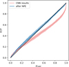 |
Fig. 2 TARP curves computed on the test set using the entire pipeline (blue line) and the feature-extracting CNN alone (red line). Shaded areas indicate the uncertainty of the curves, estimated by bootstrapping the test set. |
5 Results
In this section, we present our evaluation of the entire pipeline on the test set. A brief discussion on the performance of the CNN alone can be found in Appendix B. To evaluate how the tool is affected by the observations' resolution, we convolved the input images of the test set with Gaussian beams of four different sizes: 0, 0.1, 0.15, and 0.2 rp. We present both aggregated and separated results with regard to the synthetic image resolution.
We first test the full joint posterior inferred with DBNets2.0, then evaluate the resulting single-parameter distributions obtained by marginalising the joint. Finally, we examine and discuss the correlations between pairs of variables encoded in the inferred posteriors. To further validate our pipeline, we performed posterior predictive checks (PPC) for three elements of our test set. These involve comparing the input synthetic images to new simulations run with DBNets2.0 best estimates for the disc and planet properties. If the inference is correct, a synthetic observation generated from the inferred properties should closely reproduce the actual data. We discuss the results in Appendix C.
5.1 Full joint posterior
Figure 2 shows the result of the TARP test on the full 4D posteriors p(Mp, S t, α, h|x) inferred by our tool. The shaded area represents the uncertainty of the curve, estimated by bootstrapping the test set simulations. The expected coverage curve shows good agreement with the target diagonal, indicating that our posteriors are well calibrated (ks-pval: 0.999, atc: −0.86). The figure also shows the result of the same test performed on the summary statistics returned by the CNN, assuming that they are samples of the posterior target (ks-pval: 0.009, atc: −13.27). This highlights that Bayesian dropout on the CNN alone is insufficient in our pipeline to accurately estimate the full 4D posterior. Figure 3 presents the TARP curves separated by the input image resolution. The results demonstrate a fair agreement with the target, within the uncertainties, independent of the observational resolution.
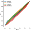 |
Fig. 3 TARP curves computed on the test set using the full pipeline, with input images convolved by Gaussian beams of varying sizes. Shaded areas indicate the uncertainty of the curves, estimated by bootstrapping the test set. |
5.2 Single parameter predictions
The accuracy of the inferred posteriors evaluated in the previous section does not necessarily imply precision. In this section, we are interested in evaluating both the accuracy and precision of single- parameter estimates that can be obtained by marginalising the full joint posterior over the other disc or planet properties. In this context, for this marginalisation, we assume uniform priors within the tool's scope of the parameter space. We define the ‘best estimate’ of a given parameter θ the median of the respective posterior p(θ|x).
Figure 4 presents metrics computed on these best estimates for each inferred property and dimension of the Gaussian beam used to convolve the input image. As noted in Sect. 5.1, the results are not significantly affected by the resolution of the input images, although a slight decrease in precision is observed at the lower resolution tested. The average standard deviation of the inferred 1D posteriors (σ in Fig. 4) is typically close to the RMSE relative to the target values, indicating that, in general, the estimated uncertainties reliably represent the actual errors.
All target properties are treated identically and are normalised to lie between −1 and 1. Therefore, these metrics indicate that planet mass can be inferred with greater precision than other properties, suggesting that the morphology of dust substructures is primarily controlled by the planet mass. Conversely, the disc scale height is the most challenging property to infer and shows a notable drop in accuracy at lower observational resolutions. For comparison, in our previous work, accounting for differences in normalisation of the target data, the RMSE of DBNets (Ruzza et al. 2024) estimates for the planet mass was 0.07 while the r2-score was 97%. Thus, within the scope and objectives of our previous work, the new pipeline achieves the same accuracy.
Figure 5 displays, for each inferred property, the distribution of samples extracted from the marginalised inferred posteriors on the test set. After binning, the 50th, 16th and 84th percentiles of these distributions are plotted as functions of the target values. The inferred parameters exhibit good agreement with the targets, which are always within the uncertainties. We observe a systematic over- and underestimation at the lower and higher end of the explored range of values, respectively, for all of the inferred properties with the exception of the planet's mass. We also performed TARP tests on these marginalised posteriors; results confirming their accuracy are shown in detail in Appendix D. While some TARP curves reveal slight biases, these are generally minor and consistent with the behaviour seen in the target-estimate plots.
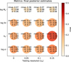 |
Fig. 4 Metrics computed on the test set for the four inferred parameters and at varying resolution of the input images. The RMSE and r2-score are computed using the median of the inferred distributions as best estimates. The σ represents the mean standard deviation of the inferred distributions. |
5.3 Correlations between pairs of variables in the inferred marginalised posteriors
One of the key advantages provided by the availability of the full joint posterior is the ability to examine correlations between disc and planet properties inferred from the substructures. These correlations arise because, typically, there is not a unique combination of disc and planet properties that determines the observed substructures; rather, several combinations can result in similar disc morphologies. To understand which properties are primarily involved in this degeneracy, we computed the Pearson correlation coefficient between all pairs of inferred variables using 5000 samples drawn from the inferred posterior for each item in our test set. The results are shown in Fig. 6. The bottom-left panels of this figure display the distribution of the computed Pearson coefficients for each pair of variables. The strongest correlations are observed between log St and log α and between log Mp and log α. Other pairs of variables also exhibit distributions of Pearson coefficients that peak away from zero, although at lower values. An interpretation of these results is given in Sect. 7.3. We also observe that these distributions are typically broad, indicating that correlations in the inferred posteriors are not consistent for all items in our test set or across the entire parameter space. This variability is illustrated in the top right panels of the figure. We note that correlation coefficients near zero, or in the opposite direction to the general trend, are usually segregated to the boundaries of the parameter space. This may be the result of a selection effect due to the low density of simulations in those regions. As with any deep learning model trained on large datasets, users should be aware that the models might be less accurate in extreme cases at the boundaries of the parameter space covered by the training data.
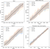 |
Fig. 5 Results on the test set for each inferred property. For each targeted disc or planet property, the plots show the correlation between DBNets2.0 estimates and target values by plotting the median of the inferred distributions along with the region between the 16th and 84th percentiles. Different colours correspond to results obtained from synthetic images at varying resolutions. |
6 Results on actual observations
We applied the newly developed pipeline to the same sample of discs with ALMA Band 6 or 7 continuum observations showing observable axisymmetric substructures, as collated in Ruzza et al. (2024). The names and properties of these objects are reported in Appendix E. In cases with multiple substructures, we applied the tool once per gap.
Aggregated results are presented in Fig. 7, and in detail for each disc in Fig. E.1. For each given input, our tool provides an estimate of the 4D posterior for the planet mass, α-viscosity, disc scale height, and dust Stokes number. To visualise and analyse these results, we sampled 5000 points θ∈ℛ4 ∼ p(θ|x) from each posterior. Figure 7 displays the distributions of the inferred properties for all 49 inputs constrained within the parameter space covered during training. Figure E.1 shows the 1D marginalised posteriors for each analysed substructure and parameter. The violin plots illustrate the posterior shape. Some cases exhibit very elongated distributions that cover the entire training scope of the tool. We interpret these results as failures to extract information about that property from the observed dust substructure.
Overall, our analysis indicates that the observed substructures imply relatively low values of α-viscosity. The inferred distribution of log α has a mean of −3.4 and standard deviation of 0.45. These results are in agreement with other constraints in the literature derived from modelling planet-disc interactions (e.g. Zhang et al. 2018, Sect. 4.4 of Rosotti 2023), and from direct measures of line broadening (e.g. Flaherty et al. 2015; Teague et al. 2016; Flaherty et al. 2020), which typically yield strong upper limits, with some exceptions, such as Flaherty et al. (2024).
We similarly observe that the distribution of inferred h0 is slightly skewed towards lower values. Since αh2 ∼ tdyn/tvisc, these results suggest generally long viscous timescales of ∼ 105− 107 Ω−1, corresponding to 106−109 yr when rescaled to the dynamical timescales (tdyn ∼ Ω−1) at the locations of the respective gaps. Plots illustrating these timescales can be found in Appendix F. Assuming a self-similar disc model, the product αh2 can be related to the star accretion rate and disc mass. Figure 8 shows, for a small sample of common objects, the viscous timescales computed in this way using disc masses from Martire et al. (2024) and mass accretion rates from Manara et al. (2014); Öberg et al. (2021). The same plot also shows local estimates of αh2 inferred with our tool from dust substructures. These local estimates are systematically lower than the global accretion timescales inferred from measurements of the star accretion rate. Variability might explain, to some extent, the higher-thanexpected accretion rates. Alternatively, the systematic nature of this difference may suggest that the local angular momentum transport mechanisms, modelled as an effective viscosity and affecting the outcome of planet-disc interactions, are insufficient to account for the global disc accretion timescales. This points towards the presence of an additional, global mechanism for dispersing angular momentum. There is considerable evidence for wind-driven angular momentum loss (see e.g. the reviews Pascucci et al. 2023; Manara et al. 2023), and the observed offset is broadly consistent with that scenario. However, caution is warranted, as we use dynamical estimates for the disc masses (Lodato et al. 2022; Longarini et al. 2025), which can only be obtained for high-mass discs, possibly introducing a selection bias into our sample.
The inferred Stokes numbers appear to be more uniformly distributed across the parameter space. However, the inferred distribution shown in Fig. 7 still exhibits a noticeable peak around St ∼ 0.03.
The dependence of the main features of planet-induced gas substructures on disc and planet properties is often expressed in terms of the coefficients K and K′, defined as
 (6)
and
(6)
and
 (7)
Specifically, several studies (e.g. Duffell & Macfadyen 2013; Kanagawa et al. 2015), using both analytical arguments and hydrodynamical simulations, have shown that the gas gap depth (Σmin/Σ0) scales approximately as 1/(1+0.04 K), while Kanagawa et al. (2016) found an empirical relation for the gap width as Δgap ∝ K′ 1/4. Figure 9 shows the overall distribution of these parameters obtained by analysing the 49 gaps in our sample of dust observations. Among other features, the K distribution exhibits a significant peak around K ∼ 10, which, according to Kanagawa et al. (2015), corresponds to planets only weakly perturbing the gas component of the disc. We compute and report these distributions because, as quantities derived from the planet-disc interaction theory, these coefficients are commonly used to study the dependence of different phenomena in this context on the disc and planet properties. For example, Scardoni et al. (2022) studied the relation between the sign of planet migration and the parameter K, identifying a threshold value of K ∼ 1.5 · 104 where the planet switches from inward to outward migration. According to this criterion, most of the proposed planet population would experience inner migration, although a significantly non-null tail of the distribution falls beyond the critical K value. However, this last observation should be interpreted with caution, as planet migration and its effects on gap morphologies (Nazari et al. 2019), were not included in our simulations.
(7)
Specifically, several studies (e.g. Duffell & Macfadyen 2013; Kanagawa et al. 2015), using both analytical arguments and hydrodynamical simulations, have shown that the gas gap depth (Σmin/Σ0) scales approximately as 1/(1+0.04 K), while Kanagawa et al. (2016) found an empirical relation for the gap width as Δgap ∝ K′ 1/4. Figure 9 shows the overall distribution of these parameters obtained by analysing the 49 gaps in our sample of dust observations. Among other features, the K distribution exhibits a significant peak around K ∼ 10, which, according to Kanagawa et al. (2015), corresponds to planets only weakly perturbing the gas component of the disc. We compute and report these distributions because, as quantities derived from the planet-disc interaction theory, these coefficients are commonly used to study the dependence of different phenomena in this context on the disc and planet properties. For example, Scardoni et al. (2022) studied the relation between the sign of planet migration and the parameter K, identifying a threshold value of K ∼ 1.5 · 104 where the planet switches from inward to outward migration. According to this criterion, most of the proposed planet population would experience inner migration, although a significantly non-null tail of the distribution falls beyond the critical K value. However, this last observation should be interpreted with caution, as planet migration and its effects on gap morphologies (Nazari et al. 2019), were not included in our simulations.
In Fig. 10, we compare the planet masses inferred using DBNets2.0 with those estimated using the previous version, DBNets (Ruzza et al. 2024; right panel) and with those proposed by Lodato et al. (2019) (left panel), who assume that the gap width scales with the planet Hill radius. In the latter case, we find good agreement between the two methods, suggesting that our tool indeed captures the morphological features of the observed substructures. Interestingly, at the higher end of the mass spectrum, DBNets2.0 tends to return lower estimates than Lodato et al. (2019). Compared to our previous work, the new estimates show good agreement for planet masses above approximately 1 MJ. For lower-mass planets, however, the correlation between the two mass estimates is weaker, with the values inferred by DBNets2.0 systematically lower than those inferred in Ruzza et al. (2024). This discrepancy may have two causes. First, tests on synthetic observations in Ruzza et al. (2024) show that the masses of low-mass planets were usually slightly overestimated. Second, observational effects, such as statistical noise or differing image resolution from that used in the training dataset, were also observed to affect mass estimates, typically leading to overestimation. Nevertheless, Ruzza et al. (2024) provided a rejection criterion to help identify such failure cases in their pipeline. In Fig. 10, we mark with yellow crosses the estimates rejected according to this criterion, observing that many of the discrepant estimates would be rejected.
Finally, in Fig. 11, we report the masses of the proposed planets in dust substructures and their radial distance from the host stars, together with all confirmed detections of exoplanets as of December 2024 (exoplanet.eu). This plot highlights how the population of young planets that would emerge from dust substructures covers a region of the Mp−a space where no exoplanets have been detected using traditional techniques, due to their intrinsic limitations. As also noted in Ruzza et al. (2024), we confirm that most (83%) of the proposed exoplanets would be sub-Jupiters (Mp<1 MJ), possibly explaining why more direct signatures of these objects have not yet been detected (Reggiani et al. 2016; Nielsen et al. 2019; Vigan et al. 2021; Asensio-Torres et al. 2021; Wallack et al. 2024).
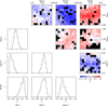 |
Fig. 6 Pearson correlation coefficients between pairs of inferred properties, computed for each element of the test set using 5000 samples from the inferred posterior. The bottom-left panels shows, for each pair of target properties, the distribution of values of the relative Pearson correlation coefficients over the entire test set. The top-right corner displays the same coefficients as a function of the two parameters considered. Bins in the 2D histograms with no data are shown in black. |
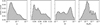 |
Fig. 7 Distribution of the inferred properties for the 49 observed substructures analysed. Each histogram is constructed by combining 5000 samples drawn from each inferred posterior. |
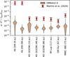 |
Fig. 8 Comparison between DBNets2.0 and literature estimates of disc viscous timescales for a subset of the analysed discs. Violin plots show the distribution of p(αh2|x) inferred with DBNets2.0. Red and green points correspond to literature estimates obtained using αh2 ∼ Ṁ/(Md Ω). Disc masses Md are dynamical measurements from Martire et al. (2024). Measures of stellar accretion rate Ṁ are from Manara et al. (2014) and Öberg et al. (2021), with an uncertainty of 0.35 dex, which dominates the αh2 uncertainties shown. |
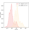 |
Fig. 9 Inferred distributions of the K and K′ coefficients for the population of proposed planets within dust substructures. The figure combines K and K′ values obtained from 5000 samples of the posterior p(α, h, St, Mp|x) for each of the 49 analysed gaps. |
7 Discussion
7.1 Independence of the results on the observation resolution
Unlike in our previous work Ruzza et al. (2024), this new pipeline was trained on synthetic observations of virtually any resolution, corresponding to a synthetic beam size between 0 and 0.2 rp. As shown in Sect. 5, the accuracy of the estimated posteriors is not influenced by the resolution of the input observation. Therefore, our tool can be safely applied to any actual observation whose beam size lies within this range. The histogram in Fig. 12 shows the distribution of beam sizes for the set of actual observations with dust substructures analysed with DBNets2.0 in Sect. 6. All fall within the scope of our tool, with only a few exceptions exhibiting slightly worse resolution.
7.2 Integration of independent constraints
Access to the full joint posterior for the target disc and planet properties enables the integration of our tool's estimates with independent constraints from other studies. For instance, we have shown the existence of a strong degeneracy between the planet's mass and the disc effective viscosity. Hence, if we were able to constrain the value of α, we could break this degeneracy and improve our estimate of the planet mass. The same also applies to the other inferred disc properties.
We showcase this capability by considering the results obtained on the 16 au gap in HD 142666, whose inferred posterior p(α, Mp|x), shown in Fig. 16, presents a marked degeneracy between the two properties, with the possible values for the viscosity spanning an entire order of magnitude. In this case, an independent measure of α could imply different estimates of the planet mass. This is shown in Fig. 13 where we plot, for this specific example, the inferred marginalised posterior for the planet mass with no constraint on α (in green) and those obtained assuming Gaussian priors with means α = 10−3 and α = 10−4 and standard deviations corresponding to a 10% error on log α. The choice of the error magnitude is discussed further in the following paragraphs. We observe that different priors on the disc viscosity cause a shift of the planet mass posterior. Additionally, we observe a slight improvement in precision with the α = 10−4 constraint, measured by a ∼ 30% reduction in the standard deviation of the distribution.
Combining independently constrained priors can thus shift the results and improve the estimates’ precision. We demonstrated this with the results obtained on a real observation constituting an ideal case because of the marked α−Mp degeneracy in the posterior and high uncertainties for both these properties. We are now interested in systematically studying the consequences of combining DBNets2.0 estimates with independent constraints in terms of both accuracy and precision. To address this, we performed the following test on the test set. First, we consider an inferred property θc and assume that another method could provide an estimate with uncertainty σc, θ. We thus represent these ‘mock’ measures as Gaussian priors  of standard deviation σc, θ and with means
  that are themselves randomly sampled from a normal distribution centred on the true value of θc (which we know because we are using synthetic observations) with standard deviation σc, θ. We then assess how imposing a constraint on θc influences the estimate of a target property θt. This is done by marginalising the 4D posteriors obtained in the test set into the 1D posteriors p(θt|x) using the prior constraints p(θc). We then compute the best estimates for θt as the medians of the 1D marginalized posteriors and evaluate their distance to the target values.
A critical aspect of this procedure is the choice of errors σc, θ assumed to be able to constrain the disc properties. If these errors exceed the typical uncertainties of our tool's estimates, little or no improvement from additional constraints would be expected. Conversely, to provide a realistic proof of concept, we note that current methods for constraining the targeted properties generally exhibit high or difficult-to-quantify uncertainties. We therefore assume an uncertainty of approximately 10% for each disc or planet property, corresponding to 0.1 in normalised units. We note that these values are smaller than the typical uncertainties of DBNets2.0 on the test set, as illustrated in Fig. 4.
The full results of this test are presented in Fig. 17 as the mean absolute error (MAE), root mean squared error (RMSE), and the mean of the posterior standard deviations (σ). We compute these metrics using the median of the inferred posteriors as the best estimate. The MAE can be compared to understand global under- or overestimations, the RMSE measures the tool's accuracy, and σ represents precision. As discussed in Sect. 4, we highlight that the RMSE computed in normalised units can be interpreted as the mean squared relative error with respect to the mean value of the range of values sampled in our training dataset (these ranges are listed in Table 1). From these values, we observe minimal or no improvement in accuracy and precision of our estimates when additional constraints on another disc property are applied. However, some notable exceptions exist. First, both α and S t benefit from constraints on the other, exhibiting slight improvements in both accuracy and precision. This outcome is expected due to the strong correlation between these properties observed in the test set results (see Sect. 5.3).
The main case warranting discussion is the planet mass estimate, which would be the main target of our tool. Figure 14 shows the error distribution for this property across cases with or without constraints on other properties. We find that, on average, an independent estimate of the disc α-viscosity would be the most helpful to reduce the uncertainty in DBNets2.0's planet mass estimates. Specifically, in the test presented here, we achieved a 15% reduction in both RMSE and σ.
All results this far were obtained using constraints for the other properties with uncertainties corresponding to a relative error of approximately 10%. In Fig. 15, we show how the RMSE of planet mass estimates would decrease if the uncertainties on the other disc properties were lower. In all cases, the RMSE would gradually decrease before eventually reaching a plateau or starting to increase again. These results show that, on average, external constraints would provide only a small increase in accuracy for the planet mass estimates. We attribute this to the already low errors and uncertainties of our tools’ estimates, which thus require very tight external constraints to yield a significant improvement. Although we demonstrated satisfactory overall accuracy, very tight priors highlight detailed regions of the inferred posteriors, requiring increasingly higher accuracy as the uncertainties of the external constraints decrease. Our posterior estimates likely lack sufficient accuracy at this level, explaining the RMSE plateau or deterioration observed in Fig. 15. However, the stage at which we observe the RMSE to remain constant (or increase) corresponds to unrealistically low errors on the other properties.
We emphasise that these results represent statistical averages over the entire test set. As noted earlier, for individual cases with large errors in one or more of the target properties, external constraints can indeed improve or alter our estimates.
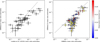 |
Fig. 10 Comparison between DBNets2.0 and literature estimates for the masses of the proposed planets in the 49 observed substructures analysed. The left-hand panel shows a comparison with Lodato et al. (2019), who assumed the gap width to scale with the planet's Hill radius. The right-hand panel presents a comparison with the estimates from the previous version of our tool, DBNets (Ruzza et al. 2024). The colour map indicates the resolution of the considered observations, measured as the beam size over the assumed planet location. The diverging colour scale is centred on the resolution used by Ruzza et al. (2024) for both training and testing. Yellow crosses mark DBNets estimates that were considered unreliable by Ruzza et al. (2024), based on their rejection criterion. |
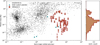 |
Fig. 11 Mass and semi-major orbital axis of the over 7000 confirmed exoplanet detections (grey points; data from exoplanet.eu). Red points mark the proposed planets in protoplanetary discs, as characterised by DBNets2.0. Error bars indicate the 16th and 84th percentiles of the inferred distributions. |
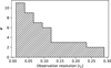 |
Fig. 12 Distribution of resolutions of the set of dust continuum observations with substructures considered in this work. |
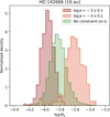 |
Fig. 13 Marginalised posteriors p(Mp|x) for the planet mass given the 16 au gap in HD 142666 with no additional constraint on α (green histogram), and setting Gaussian priors for log α centred at −3 (dark red histogram) or −4 (orange histogram), each with a standard deviation of 0.1. Means mu and standard deviations σ of the shown distributions are: μ=−3.82, σ=0.11 (no constraint on α); μ=−3.60; σ=0.11 (α = 10−3); and μ=−3.96, σ=0.08(α = 10−4). |
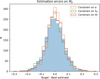 |
Fig. 14 Distributions of errors of DBNets best estimates (medians of the inferred posteriors) for the planet mass obtained with and without prior constraints on the other target properties. The test was performed on the test set. |
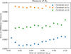 |
Fig. 15 Root mean squared error (RMSE) of the planet mass estimates obtained by integrating the tool's results with external constraints on one of the other inferred properties, shown as a function of the assumed uncertainty of the independent constraint. |
7.3 Observed degeneracies and comparison with literature results
In Sect. 5.3, we discussed the correlation between disc and planet properties, as captured by the posteriors inferred on the test set. These correlations can be interpreted by considering that the same morphological features of dust substructures can be obtained with different combinations of properties. To provide a general but quantitative picture, we consider each pair of target properties (e.g. Mp and α) and assume that the degeneracy between them can be described by a power law, Mp ∝ αγ. This implies that, within a certain domain, systems with individually different values of Mp and α can present the same morphology if the power-law relation holds with the same multiplicative coefficient. We therefore consider each pair of properties and measure the possible indices of these degeneracies by fitting the marginalised posteriors in the logged parameter space with a bivariate Gaussian distribution, and computing the slope of its semi-major axis. This is the line along which all points would lie in the limit of ρ → 1, where ρ denotes the Pearson correlation coefficient. In general, ρ is the cosine of the angle between the two separate best linear predictors of one variable with respect to the other. Hence, the most reliable dependence between the two variables is given by the distributions with the highest ρ. In Fig. 18, we show the slopes obtained in this way as a function of ρ for the respective distributions. We also show, in the same plot, three examples of the marginalised 2D posteriors relative to the lower, median, and highest correlation coefficients, to visually assess the meaning of these values in terms of the distribution's shape. For each pair of properties, we provide a single estimate, with uncertainties, for the index of the possible power-law degeneracy, averaging the slopes computed for each element of the test set, weighted by the square of their Pearson correlation coefficient.
It is interesting to examine whether these relations correspond to those captured by the K and K′ coefficients (introduced in Sect. 6), which have been found to capture the main dependence of gap morphologies on the properties of the disc and the planet. The slope we measure for the typical correlation between Mp and α in our test set (Mp ∝ α0.42) is in good agreement with the degeneracy captured by both the K and K′ coefficients which, when other properties are fixed, would result in Mp ∝ α1/2. The measured, nearly linear, relation between α and St is compatible with the substructures’ morphologies being primarily determined by the ratio of St to α, rather than by the two properties separately. Analogously, the relation Mp ∝ St0.52 ± 0.35 supports this picture, with an index compatible with that between Mp and α. This suggests that the main morphological features used in the inference are those associated with dust trapping, specifically those related to the rings.
Considering the Mp−h degeneracy, the mean power-law index that we measure in this case (2.66) is in good agreement with that expected from the K coefficient. However, we observe greater scatter and typically lower correlation coefficients, indicating that this degeneracy is weaker and less coherent across different regions of the parameter space. Some of the scatter may be explained by the differing dependence of the K and K′ coefficients on the disc aspect ratio. These are related, respectively, to the gap depth and width, which should be simultaneously taken into account by the CNN in our pipeline.
Although less pronounced, some scatter is also observed in both the correlation coefficients and the measured power-law indices in the other cases. We note that the empirical relations based on the K and K′ are derived from morphological features of gas gaps, whereas in this work we consider only dust substructures. We expect these formulae to remain approximately valid due to the low Stokes numbers of our simulations, but it may also explain the imperfect agreement with analytical expectations and the absence of a unique parameter degeneracy. Furthermore, we estimate the expected degeneracies between pairs of parameters based on the empirical formulae by fixing all the other properties, but we measure them on the 2D marginalised posterior distributions. Hence, if the integrated properties are not completely independent, an uncertainty on them could obscure or alter the relation between the two properties under examination. A more systematic study of how these relations vary across the parameter space, and of their multidimensional dependences, is beyond the scope of this paper.
 |
Fig. 16 DBNets 2.0 inferred posterior for the α-viscosity and planet mass given the gap at 16 au in HD 14266. |
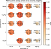 |
Fig. 17 Evaluation metrics for each inferred property with and without a sharp Gaussian prior on a different property, with standard deviation corresponding to a 10% uncertainty. In each case, we report the mean absolute errors (MAE), indicative of overall biases, the root mean squared error (RMSE) indicative of the tool's accuracy, and the mean standard deviation of the inferred posteriors (σ, indicative of the tool's precision). The size of the markers is proportional to σ. |
8 Conclusion
In this work, we developed a simulation-based inference pipeline for the analysis of protoplanetary disc observations of dust thermal emission. From the morphology of the observed substructures, we estimate the posterior for the disc α-viscosity, disc scale height, dust Stokes number, and the mass of a putative planet. This is the first publicly available and fully automated tool with this capability. We performed TARP tests (Lemos et al. 2023a) and computed standard metrics (RMSE and r2-score) to quantify the accuracy and precision of the inferred posteriors.
With respect to our previous work Ruzza et al. (2024), the most significant improvement lies in the inference of the full posterior for the planet mass and additional disc properties. We also resolved two minor issues, providing a new pipeline whose accuracy is not affected by the resolution of the input observation or by the position of the outer disc edge. Additionally, DBNets could only approximate the inferred posterior as a Gaussian mixture, whereas in this work we were able to remove this limitation through the use of normalising flows. In the test set, we achieve an RMSE for the planet mass of 0.07 which, taking into account the different normalisation, is consistent with the results obtained in our previous work (Ruzza et al. 2024). In actual observations, the DBNets and DBNets2.0 planet mass estimates are in good agreement at the higher end of the mass spectrum. For lower masses, we typically infer lower values with the new pipeline. This result is consistent with the tests performed in Ruzza et al. (2024), where we observed a systematic overestimation of low planet masses in synthetic observations, particularly after the injection of observational errors (e.g. noise, deprojection effects, or change of resolution).
Evaluating our tool's precision on the test set, we conclude that the morphology of planet-induced substructures is primarily determined by the planet mass, as this is always the best-constrained property. Nevertheless, the other properties are also inferred successfully, with errors significantly lower than the parameter space dimension, suggesting that they also imprint detectable signatures on the substructures’ morphologies. We also studied, using the same results, the degeneracies captured by the inferred posteriors between each pair of parameters, finding α and St to be the properties with the most marked degeneracy with the planet mass. A strong correlation between α and St themselves, consistent with α ∝ St, suggests that, in addition to the planet mass, the morphology of dust substructures is primarily controlled by the ratio between these two properties.
We applied the developed pipeline to a set of 49 gaps across 34 discs, independently assuming the presence of a planet in each gap. The results indicate generally low α-viscosities and disc scale heights, which would imply long viscous timescales (∼ 105−107 Ω−1). The population of proposed planets also exhibits generally low masses, with approximately 83% of them below 1 MJ, consistent with the lack of direct detections of these objects.
The pipeline presented here demonstrates an approach to fitting a simulation-based model to data, with techniques that improve both speed and accuracy compared to alternative procedures. The inferred posteriors should be interpreted with caution, as they represent results conditioned on the model and assumptions underlying the synthetic observations used in the training dataset. As such, they do not account for situations or phenomena not included in these simulations. Future work could improve the underlying models by introducing additional effects, such as planet migration, dust feedback, or planet multiplicity. In this scenario, access to the full posteriors for the disc and planet properties, rather than single value best estimates, would allow us to perform a rigorous statistical comparison of different models to determine which best fits the data.
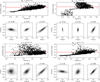 |
Fig. 18 Degeneracies between pairs of properties highlighted by the inferred posteriors on the test set. For each simulation, these plots show the slope of the major axis of the 2D Gaussian that best fits the inferred posterior as a function of the Pearson correlation coefficients. Higher correlation coefficients correspond to sharper distributions towards the major axis of the Gaussian ellipses, as shown by the exemplificative examples plotted. As indicated by the plot titles, the inferred slopes suggest possible degeneracies between pairs of properties in forming the observed substructures. The red lines indicate the weighted average slope, calculated using the Pearson coefficients as weights. |
Data availability
The entire pipeline is publicly available as a Python package at https://github.com/dust-busters/DBNets. DBNets2.0 requires a disc observation of the dust continuum, the disc's geometrical properties (inclination, position angle, and location of the disc centre within the image), and an estimate on the suspected planet's location, provided either as the angular separation from the disc centre or in physical units using the disc distance. The tool then returns the best-fitting posterior distribution for the planet mass, disc viscosity, aspect ratio, and dust Stokes number. Utility functions are also provided to interpret and analyse the results. Comprehensive documentation, including commented examples, is available via the same link.
Acknowledgements
We thank the anonymous referee for the insightful comments and suggestions. Computational resources have been provided by the INDACO Core facility, which is a project of High Performance Computing at the Università degli Studi di Milano (https://www.unimi.it). We also acknowledge ISCRA for awarding this project access to the LEONARDO supercomputer, owned by the EuroHPC Joint Undertaking, hosted by CINECA (Italy). This work has been supported by Fondazione Cariplo, grant no. 2022-1217, from the European Union's Horizon Europe Research & Innovation Programme under the Marie Sklodowska-Curie grant agreement No. 823823 (DUSTBUSTERS) and from the European Research Council (ERC) under grant agreement no. 101039651 (DiscEvol). GL acknowledges support from PRIN-MUR 20228JPA3A and from the European Union Next Generation EU, CUP:G53D23000870006. Views and opinions expressed are however those of the author(s) only, and do not necessarily reflect those of the European Union or the European Research Council Executive Agency. Neither the European Union nor the granting authority can be held responsible for them.
Appendix A Confidence score
DBNets2.0 is a simulation-based inference tool. As such, it infers the posterior distribution for some target properties, fitting data with a model that is intrinsically defined by the training synthetic data. This means that the results are dependent on all the assumptions made in running the simulations used to generate these data and on the structure of the explored parameter space. Data that satisfy these assumptions and therefore are within the scope of the tool are typically referred to as in-distribution (ID) data in opposition to out-of-distribution (OOD) data, which are instead out of the tool's scope. Deep learning methods, like those we used in our SBI pipeline, are designed to interpolate within ID data but are typically not reliable when applied to OOD data. While directly detecting OOD data is challenging, as most of the assumptions made in generating the training dataset cannot be directly and reliably assessed, we can instead check the similarity of the data that we are targeting with the training data. Although this approach does not eliminate the possibility of degeneracies with OOD scenarios, it provides a practical means to estimate the reliability of the model's outputs. Following this idea, we designed and equipped our tool with the “confidence score” (CS), a new metric that helps the user to assess the reliability of the inferred posterior.
The idea underlying this metric is to quantify the difference between the input observation and a synthetic observation corresponding to DBNets2.0 best estimates for the disc and planet properties. In other words, this metric summarises in a faster and automated procedure the PPC tests presented in Appendix C. Given an observation x and DBNets2.0 estimate p(θ|x), CS is computed as follows: 1) we sample ten θi from.p(θ|x), 2) we linearly interpolate the synthetic images in the training dataset at all θi, 3) we remap the interpolated images bi and the input image x to polar coordinates, 4) we compute the FFT of the remapped bi and x, 5) we compute CS as
 (A.1)
This pipeline implements the idea previously exposed. We use linear interpolation of the training dataset as a cheap surrogate of hydrodynamical simulations, but we sample 10 points from the inferred posterior to average out artefacts and errors. Additionally, sampling 10 points also makes the CS definition sensitive to the uncertainty of the inferred properties, lowering its value in the case of broad inferred posteriors. We remap the images to polar coordinates and compute the Fourier decomposition, using only the modulus of the complex Fourier coefficients, to remove any azimuthal dependence. For instance, if the input data presents a strong azimuthal asymmetry the image is found similar to the training data if a similar asymmetry is present, regardless of its azimuthal position. We finally included a normalisation factor in our definition of CS.
(A.1)
This pipeline implements the idea previously exposed. We use linear interpolation of the training dataset as a cheap surrogate of hydrodynamical simulations, but we sample 10 points from the inferred posterior to average out artefacts and errors. Additionally, sampling 10 points also makes the CS definition sensitive to the uncertainty of the inferred properties, lowering its value in the case of broad inferred posteriors. We remap the images to polar coordinates and compute the Fourier decomposition, using only the modulus of the complex Fourier coefficients, to remove any azimuthal dependence. For instance, if the input data presents a strong azimuthal asymmetry the image is found similar to the training data if a similar asymmetry is present, regardless of its azimuthal position. We finally included a normalisation factor in our definition of CS.
A.1 Validation and calibration
To calibrate this confidence score and assess its correct functioning we performed several tests. First, we checked CS values for input data completely out of scope, i.e. white noise, observing, as shown in Fig. A.1, that their distribution is well separated from that of CS values computed for our validation set. Furthermore, in Fig. A.2 we compare the CS values computed for the test set images augmented with the same augmentation layers used in the DBNets2.0 CNN (see Sect. 3.2) using the same (ID) and wider (OOD) ranges for the augmentation hyperparameters (e.g. translation factor, noise level, synthetic resolution, etc.). We observe a shift of CS values towards lower values in the case of inputs on which OOD augmentation was performed. Note that while in the case of OOD augmentation we increased the ranges of allowed values for the augmentation's hyperparameters, these are randomly sampled for each new observation and might thus, in specific cases, still fall within ID values. Additionally, particularly simple morphologies might still appear similar to the training data even when OOD augmentation is performed. This explains the overlap in the CS values distributions.
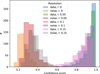 |
Fig. A.1 Confidence score distributions for DBNets2.0 estimates on the synthetic observations of the test set and on white noise images. In both cases, we show the results for the same images convolved with a Gaussian beam of different sizes (standard deviation reported in the legend). |
From the results shown in Fig. A.1 and Fig. A.2 we can suggest a threshold of 0.6 for CS under which DBNets2.0 estimates should be rejected. However, we strongly encourage future users to consider the actual CS value, treating it exactly as a continuous confidence score whose value must be considered together with all the information available about the disc under exam. Indeed, individually inspecting the disc morphologies, we observe that they become qualitatively more peculiar as the CS decreases. For instance, Fig. A.3 shows the 9 elements of the validation set corresponding to the lowest CS. As shown, these exhibit untypical morphologies with strong asymmetries or multiple rings and gaps.
As a final test, we computed the CS on synthetic observations generated from simulations with two planets. This is meant to benchmark the CS in a case where the physics assumptions in the model that DBNets2.0 is fitting are not met. Figure A.4 shows these synthetic images ordered with respect to the CS of DBNets2.0 estimate. We observe that even though none of these CS values fall below 0.6, the images corresponding to the lowest CS exhibit the most peculiar morphologies with multiple gaps and rings that are probably difficult to explain with only one planet. It is, however, important to keep in mind that this metric cannot point out degeneracies with OOD systems, and therefore, generally, a high CS is still expected if the observed morphology could also be explained with only one planet.
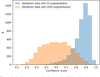 |
Fig. A.2 Confidence score distributions for DBNets2.0 estimates on the synthetic observations of the test set randomly augmented with the same augmentation layers used during training: random rotation, random translation, random cut of the outer disc, convolution with a Gaussian beam of random size and addition of white noise. The blue histogram corresponds to in-distribution (ID) augmentation, i.e. using the same hyperparameters used during training. The orange histogram corresponds to values obtained for images on which we performed OOD augmentation increasing the maximum translation factor from 0.01 to 0.1, the noise standard deviation from 0.1 to 0.2 and the maximum synthetic beam size from 0.2 to 0.4 (in code units). |
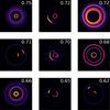 |
Fig. A.3 Morphology of the substructures in the test set synthetic observations corresponding to the lowest confidence scores (reported in the upper right corner of each image). |
A.2 Confidence score of DBNets2.0 application to actual observations
We show in Fig. A.5 the distribution of CS obtained for the actual observations on which we applied DBNets2.0 in this paper. Figure A.6 shows the morphology of the observed substructures ordered with respect to the obtained CS. We also report CS values for each DBNets2.0 estimate in Table E.1.
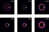 |
Fig. A.4 Synthetic observations obtained from hydrodynamical simulations with two planets. The confidence score of DBNets2.0 estimates on these images is reported in the upper right corners. In each image, the star marks the position of the planet which is also assumed for the analysis of DBNets2.0, while the point marks the position of the second planet in the simulation. |
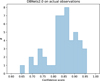 |
Fig. A.5 Distribution of confidence scores obtained for DBNets2.0 estimates on the actual observations analysed in this paper and listed in Table E.1. |
 |
Fig. A.6 Deprojected continuum observations of actual discs analysed with DBNets2.0 in this paper. Images are ordered according to the confidence score of DBNets2.0 estimate and are meant to show how this metric relates to the observations’ features. |
Appendix B Evaluation of the feature extracting CNN (first step of the pipeline)
Figure B.1 shows the learning curve (i.e. loss function as a function of the training epoch) of the CNN trained in this work. The black line shows the loss function computed on the training dataset while the others refer to the loss function computed on the test set with synthetic images convolved with Gaussian beams of different dimensions where darker colours refer to smaller beams. We observe that the CNN is trained effectively exhibiting a significant lowering of the loss function evaluated on the training set. The test set curves show that the CNN is not overtrained. Beyond the stochastic behaviour, a small but sys- tematic improvement of these curves can be observed up to the last training epochs. We remind that the CNN output, for each input observation, is a set of 4 real values interpreted as estimates of log α, h, log St and log Mp. Enabling dropout layers during inference, we collect for each input a set of 1500 estimates for each target property which, in our pipeline, are used as input to the normalising flows. A different solution could have been to directly interpret these values as samples extracted from the target posterior distribution p(α, h, St, Mp|x). We already show in Sect. 5.1, performing the TARP test, that this method would provide inaccurate estimates. We additionally report here in Fig. B.2 some metrics analogously to Fig. 4 but computed using only the CNN outputs. The rmse values are all systematically higher than the σ values, which correspond to the standard deviations of the distributions obtained from the CNN outputs, indicating that these systematically underestimate the uncertainties.
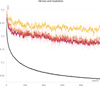 |
Fig. B.1 Loss function (mse averaged over all 4 inferred parameters) computed during training for both the training and test sets. The black line refers to the metric computed on the training dataset. Coloured lines refer to the metric computed on the test set where each image has been convolved with a Gaussian beam of fixed size among [0, 0.05, 0.1, 0.15] rp. Darker colours correspond to smaller beam sizes. Plots are shown for one of the 5 folds trained but the others exhibit a similar behaviour. |
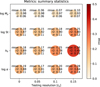 |
Fig. B.2 Different metrics summarising the CNN results on the test set for each inferred parameter and for different synthetic resolutions. The colours ascend from brighter to darker as the mse. Sizes scale as σ. Definitions of the plotted metrics can be found in the text (Appendix B). |
Appendix C Posterior predictive check
In this appendix, we present the results of posterior predictive checks (PPC; e.g. Gabry et al. 2019) that we used to further test our pipeline. In a PPC, one considers the observed data x0 and compares them with those generated from the pipeline's best estimates of the target properties. We call “best estimates” the medians of the inferred marginalised posterior distributions corresponding also, in all these cases, to the maximum a posteriori estimate (MAP). The general idea is that the generated data should look similar to the observed one if the inference is correct. We performed this test using synthetic observations and selected examples with a large difference between the target properties and their inferred best estimates. These are the most interesting to perform this test as they can show if the inferred posteriors are correctly tracing degeneracies between parameters. Instead, if the best estimates were close to the actual target values, the test would be comparing synthetic observations that are expected to be similar because obtained from simulations with small differences in their disc and planet properties.
Figure C.1 shows the results of three iterations of this test (one per row) for three different synthetic observations. The corner plots in the left panel show the inferred posterior distributions (black histograms with medians in orange) compared to the “true” values of the target properties (blue lines). Note that these mostly lie in the tail of the inferred posteriors. In the right panel we compare the simulated dust distributions with the “true” values and best estimates of the system's properties. We observe a good agreement both in the 2D map and in the azimuthally averaged radial profile. The main noticeable difference is in the value of the dust density in the gap minimum which, in all three cases, appears lower in the simulation with the inferred best estimates of the disc and planet properties. This difference, however, being orders of magnitude lower than the gap depth, is practically negligible. The third case presents the most significant difference of the synthetic observation generated with the MAP properties with respect to the original. This is probably due to the low target viscosity close to the lower end of the explored parameter space. Therefore, although the target value is still plausible according to the inferred posterior, its best estimate is slightly higher causing also, as a consequence, a shift of the best estimates of the other properties.
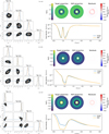 |
Fig. C.1 Results of three posterior predictive checks. Each row corresponds to a PPC considering a different synthetic observation in the test set. Left panel: corner plots showing the inferred posterior distributions for the target properties. The orange lines mark the medians of the marginalised posteriors for each target property which are then assumed as the respective best estimates. The blue lines mark the target “true” values. Confidence scores (CS) of DBNets2.0 estimates (see appendix A) are reported in the upper right corners. Right panel: comparison between the simulated dust distributions with the “true” and “best estimates” values of the systems’ properties. Both the 2D distribution (upper panels) and the azimuthally averaged radial profile of the dust density (lower panels) are compared. |
Appendix D TARP on single parameters marginalised posteriors
We report in Fig. D.1 the results of TARP tests performed, for the test set, on the inferred posteriors marginalised for all but one target property.
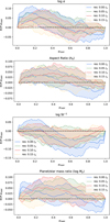 |
Fig. D.1 Results of TARP tests performed for each target property on the marginalised distributions over the other parameters. The different colours refer to the results obtained on synthetic observations convolved with different beam sizes. The dashed black lines mark the target curves that would be obtained if the inferred posteriors were perfectly accurate. |
Appendix E Set of continuum observations considered and DBNets2.0 inference results
In Table E.1 we list the name and properties of the 34 protoplanetary disc observations on which we applied our tool in Sect. 6. We also report in the same table DBNets2.0 estimates of the targeted properties with uncertainties marking the 16th and 84th percentiles of the respective marginalised distributions. DBNets2.0 estimates for each disc are also shown with violin plots in Fig. E.1.
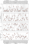 |
Fig. E.1 Overview of the best estimates of each target property for all the 49 dust substructures considered. The grey violin plots represent the inferred posterior distributions marginalised over all other parameters. The red squares mark the medians of these distributions. |
Catalogue of ALMA observations on which we applied DBNets2.0.
Appendix F Inferred viscous timescales
We show in Fig. F.1 the distribution of (αh2)−1 inferred with DBNets2.0 from the set of dust observations considered in this work. As explained in the main text, this quantity can be interpreted as the ratio between the dynamical and viscous timescales measured locally at the gap location. In Fig. F.2 we provide the same distribution for the viscous timescale in years rescaling for the appropriate dynamical timescales.
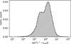 |
Fig. F.1 Inferred distribution of (αh2)−1 ∼ tvisc Ω for the population of proposed planets within dust substructures. The plot is made extracting 5000 samples for α and h from the inferred p(α, h, S t, Mp|x) for each of the 49 analysed gaps. |
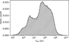 |
Fig. F.2 Inferred distribution of tvisc for the population of proposed planets within dust substructures. The plot is made extracting 5000 samples for α and h from the inferred p(α, h, S t, Mp|x) for each of the 49 analysed gaps and computing tvisc as tvisc = 1/(Ω αh2). |
References
- Abadi, M., Agarwal, A., Barham, P., et al. 2015, arXiv e-prints [arXiv:1603.04467] [Google Scholar]
- Andrews, S. M., Wilner, D. J., Zhu, Z., et al. 2016, AJ, 820, L40 [Google Scholar]
- Andrews, S. M., Huang, J., Pérez, L. M., et al. 2018, ApJ, 869, L41 [NASA ADS] [CrossRef] [Google Scholar]
- Asensio-Torres, R., Henning, T., Cantalloube, F., et al. 2021, A&A, 652, A101 [NASA ADS] [CrossRef] [EDP Sciences] [Google Scholar]
- Auddy, S., Dey, R., Lin, M.-K., Carrera, D., & Simon, J. B., 2022, ApJ, 936, 93 [NASA ADS] [CrossRef] [Google Scholar]
- Auddy, S., & Lin, M.-K., 2020, AJ, 900, 62 [Google Scholar]
- Auddy, S., Dey, R., Lin, M.-K., & Hall, C., 2021, ApJ, 920, 3 [NASA ADS] [CrossRef] [Google Scholar]
- Bae, J., Isella, A., Zhu, Z., et al. 2023, ASP Conf. Ser., 534, 423 [NASA ADS] [Google Scholar]
- Barge, P., Ricci, L., Carilli, C. L., & Previn-Ratnasingam, R., 2017, A&A, 605, A122 [NASA ADS] [CrossRef] [EDP Sciences] [Google Scholar]
- Baruteau, C., Barraza, M., Pérez, S., et al. 2019, MNRAS, 486, 304 [Google Scholar]
- Benisty, M., Bae, J., Facchini, S., et al. 2021, ApJ, 916, L2 [NASA ADS] [CrossRef] [Google Scholar]
- Benitez-Llambay, P., & Masset, F. S., 2016, AJ Suppl. Ser., 223, 11 [Google Scholar]
- Benítez-Llambay, P., Krapp, L., & Pessah, M. E., 2019, AJ Suppl. Ser., 241, 25 [Google Scholar]
- Chollet, F., et al. 2015, Keras, https://keras.io [Google Scholar]
- Christiaens, V., Cantalloube, F., Casassus, S., et al. 2019, ApJ, 877, L33 [Google Scholar]
- Clarke, C. J., Tazzari, M., Juhasz, A., et al. 2018, AJ, 866, L6 [Google Scholar]
- Currie, T., Lawson, K., Schneider, G., et al. 2022, Nat. Astron., 6, 751 [NASA ADS] [CrossRef] [Google Scholar]
- Dipierro, G., & Laibe, G., 2017, MNRAS, 469, 1932 [Google Scholar]
- Dipierro, G., Price, D., Laibe, G., et al. 2015, MNRAS, 453, L73 [NASA ADS] [CrossRef] [Google Scholar]
- Dong, R., & Fung, J., 2017, AJ, 835, 146 [Google Scholar]
- Dong, R., Li, S., Chiang, E., & Li, H., 2018, AJ, 866, 110 [Google Scholar]
- Duffell, P. C., & Macfadyen, A. I., 2013, AJ, 769, 41 [Google Scholar]
- Dullemond, C. P., & Penzlin, A. B. T., 2018, A&A, 609, A50 [NASA ADS] [CrossRef] [EDP Sciences] [Google Scholar]
- Facchini, S., Benisty, M., Bae, J., et al. 2020, A&A, 639, A121 [EDP Sciences] [Google Scholar]
- Fedele, D., Tazzari, M., Booth, R., et al. 2018, A&A, 610, A24 [NASA ADS] [CrossRef] [EDP Sciences] [Google Scholar]
- Fedele, D., Bollati, F., & Lodato, G., 2023, A&A, 672, A125 [NASA ADS] [CrossRef] [EDP Sciences] [Google Scholar]
- Flaherty, K. M., Hughes, A. M., Rosenfeld, K. A., et al. 2015, AJ, 813, 99 [Google Scholar]
- Flaherty, K., Hughes, A. M., Simon, J. B., et al. 2020, AJ, 895, 109 [Google Scholar]
- Flaherty, K., Hughes, A. M., Simon, J. B., et al. 2024, MNRAS, 532, 363 [NASA ADS] [CrossRef] [Google Scholar]
- Gabry, J., Simpson, D., Vehtari, A., Betancourt, M., & Gelman, A., 2019, J. R. Stat. Soc. Ser., 182, 389 [Google Scholar]
- Gal, Y., & Ghahramani, Z., 2016, Proceedings of The 33rd International Conference on Machine Learning, eds. M. F. Balcan & K. Q. Weinberger (New York, USA: PMLR), 48, 1050 [Google Scholar]
- Gratton, R., Ligi, R., Sissa, E., et al. 2019, A&A, 623, A140 [NASA ADS] [CrossRef] [EDP Sciences] [Google Scholar]
- Haffert, S. Y., Bohn, A. J., de Boer, J., et al. 2019, Nat. Astron., 3, 749 [Google Scholar]
- Hammond, I., Christiaens, V., Price, D. J., et al. 2023, MNRAS, 522, L51 [NASA ADS] [CrossRef] [Google Scholar]
- Hashimoto, J., Muto, T., Dong, R., et al. 2021, AJ, 911, 5 [Google Scholar]
- Hawley, J. F., 2001, AJ, 554, 534 [Google Scholar]
- He, K., Zhang, X., Ren, S., & Sun, J., 2016, in 2016 IEEE Conference on Computer Vision and Pattern Recognition (CVPR), 1 [Google Scholar]
- Hu, X., Zhu, Z., Okuzumi, S., et al. 2019, ApJ, 885, 36 [Google Scholar]
- Huang, J., Andrews, S. M., Dullemond, C. P., et al. 2020a, AJ, 891, 48 [Google Scholar]
- Huang, J., Andrews, S. M., Öberg, K. I., et al. 2020b, AJ, 898, 140 [Google Scholar]
- Isella, A., Guidi, G., Testi, L., et al. 2016, PRL, 117, 251101 [Google Scholar]
- Isella, A., Benisty, M., Teague, R., et al. 2019, AJ, 879, L25 [Google Scholar]
- Kanagawa, K. D., Tanaka, H., Muto, T., Tanigawa, T., & Takeuchi, T., 2015, MNRAS, 448, 994 [NASA ADS] [CrossRef] [Google Scholar]
- Kanagawa, K. D., Muto, T., Tanaka, H., et al. 2016, PASJ, 68, 43 [NASA ADS] [Google Scholar]
- Kendall, A., & Gal, Y., 2017, Advances in Neural Information Processing Systems, 5575 [Google Scholar]
- Keppler, M., Teague, R., Bae, J., et al. 2019, A&A, 625, A118 [NASA ADS] [CrossRef] [EDP Sciences] [Google Scholar]
- Kim, S., Takahashi, S., Nomura, H., et al. 2020, AJ, 888, 72 [Google Scholar]
- Le Folgoc, L., Baltatzis, V., Desai, S., et al. 2021, arXiv e-prints [arXiv:2110.04286] [Google Scholar]
- Lemos, P., Coogan, A., Hezaveh, Y., & Perreault-Levasseur, L. 2023a, 40th International Conference on Machine Learning, 202, 19256 [Google Scholar]
- Lemos, P., Parker, L. H., Hahn, C., et al. 2023b, in Machine Learning for Astrophysics, 18 [Google Scholar]
- Lodato, G., Dipierro, G., Ragusa, E., et al. 2019, MNRAS, 486, 453 [Google Scholar]
- Lodato, G., Rampinelli, L., Viscardi, E., et al. 2022, MNRAS, 518, 4481 [NASA ADS] [CrossRef] [Google Scholar]
- Long, F., Pinilla, P., Herczeg, G. J., et al. 2018, AJ, 869, 17 [Google Scholar]
- Longarini, C., Lodato, G., Rosotti, G., et al. 2025, ApJ, 984, L17 [Google Scholar]
- Manara, C. F., Testi, L., Natta, A., et al. 2014, A&A, 568, A18 [NASA ADS] [CrossRef] [EDP Sciences] [Google Scholar]
- Manara, C. F., Ansdell, M., Rosotti, G. P., et al. 2023, ASPC, 534, 539 [Google Scholar]
- Mao, S., Dong, R., Lu, L., et al. 2023, ApJ, 950, L12 [CrossRef] [Google Scholar]
- Mao, S., Dong, R., Yi, K. M., et al. 2024, ApJ, 976, 200 [Google Scholar]
- Marino, S., 2021, MNRAS, 503, 5100 [NASA ADS] [CrossRef] [Google Scholar]
- Martire, P., Longarini, C., Lodato, G., et al. 2024, A&A, 686, A9 [Google Scholar]
- Mesa, D., Keppler, M., Cantalloube, F., et al. 2019, A&A, 632, A25 [NASA ADS] [CrossRef] [EDP Sciences] [Google Scholar]
- Nazari, P., Booth, R. A., Clarke, C. J., et al. 2019, MNRAS, 485, 5914 [Google Scholar]
- Nielsen, E. L., De Rosa, R. J., Macintosh, B., et al. 2019, AJ, 158, 13 [Google Scholar]
- Öberg, K. I., Guzmán, V. V., Walsh, C., et al. 2021, ApJS, 257, 1 [CrossRef] [Google Scholar]
- Pascucci, I., Cabrit, S., Edwards, S., et al. 2023, ASPC, 534, 567 [Google Scholar]
- Pérez, S., Casassus, S., Baruteau, C., et al. 2019, AJ, 158, 15 [Google Scholar]
- Pinte, C., 2019, HD 97048 ALMA B7 continuum + 13CO, https://doi.org/10.6084/m9.figshare.8266988.v1 [Google Scholar]
- Pinte, C., van der Plas, G., Ménard, F., et al. 2019, Nat. Astron., 3, 1109 [NASA ADS] [CrossRef] [Google Scholar]
- Reggiani, M., Meyer, M. R., Chauvin, G., et al. 2016, A&A, 586, A147 [NASA ADS] [CrossRef] [EDP Sciences] [Google Scholar]
- Rosotti, G. P., 2023, New Astron. Rev., 96, 101674 [NASA ADS] [CrossRef] [Google Scholar]
- Rosotti, G. P., Juhasz, A., Booth, R. A., & Clarke, C. J., 2016, MNRAS, 459, 2790 [Google Scholar]
- Ruzza, A., Lodato, G., & Rosotti, G. P., 2024, A&A, 685, A65 [NASA ADS] [CrossRef] [EDP Sciences] [Google Scholar]
- Scardoni, C. E., Clarke, C. J., Rosotti, G. P., et al. 2022, MNRAS, 514, 5478 [NASA ADS] [CrossRef] [Google Scholar]
- Teague, R., Guilloteau, S., Semenov, D., et al. 2016, A&A, 592, A49 [CrossRef] [EDP Sciences] [Google Scholar]
- Tejero-Cantero, A., Boelts, J., Deistler, M., et al. 2020, J. Open Source Softw., 5, 2505 [NASA ADS] [CrossRef] [Google Scholar]
- Toci, C., Lodato, G., Fedele, D., Testi, L., & Pinte, C., 2019, AJ, 888, L4 [Google Scholar]
- Toci, C., Lodato, G., Christiaens, V., et al. 2020, MNRAS, 499, 2015 [NASA ADS] [CrossRef] [Google Scholar]
- van Terwisga, S. E., van Dishoeck, E. F., Ansdell, M., et al. 2018, A&A, 616, A88 [NASA ADS] [CrossRef] [EDP Sciences] [Google Scholar]
- Veronesi, B., Ragusa, E., Lodato, G., et al. 2020, Eur. Planet. Sci. Congress, 2020–398 [Google Scholar]
- Vigan, A., Fontanive, C., Meyer, M., et al. 2021, A&A, 651, A72 [EDP Sciences] [Google Scholar]
- Wagner, K., Follette, K. B., Close, L. M., et al. 2018, ApJ, 863, L8 [NASA ADS] [CrossRef] [Google Scholar]
- Wallack, N. L., Ruffio, J.-B., Ruane, G., et al. 2024, AJ, 168, 78 [Google Scholar]
- Wang, S., Kanagawa, K. D., & Suto, Y., 2021, AJ, 923, 165 [Google Scholar]
- Zhang, S., Zhu, Z., Huang, J., et al. 2018, AJ, 869, L47 [Google Scholar]
- Zhang, S., Zhu, Z., & Kang, M., 2022, MNRAS, 510, 4473 [NASA ADS] [CrossRef] [Google Scholar]
- Zhou, Y., Bowler, B. P., Wagner, K. R., et al. 2021, AJ, 161, 244 [NASA ADS] [CrossRef] [Google Scholar]
All Tables
All Figures
|
Fig. 1 Schematic of DBNets2.0 pipeline and objective. |
| In the text | |
|
Fig. 2 TARP curves computed on the test set using the entire pipeline (blue line) and the feature-extracting CNN alone (red line). Shaded areas indicate the uncertainty of the curves, estimated by bootstrapping the test set. |
| In the text | |
|
Fig. 3 TARP curves computed on the test set using the full pipeline, with input images convolved by Gaussian beams of varying sizes. Shaded areas indicate the uncertainty of the curves, estimated by bootstrapping the test set. |
| In the text | |
|
Fig. 4 Metrics computed on the test set for the four inferred parameters and at varying resolution of the input images. The RMSE and r2-score are computed using the median of the inferred distributions as best estimates. The σ represents the mean standard deviation of the inferred distributions. |
| In the text | |
|
Fig. 5 Results on the test set for each inferred property. For each targeted disc or planet property, the plots show the correlation between DBNets2.0 estimates and target values by plotting the median of the inferred distributions along with the region between the 16th and 84th percentiles. Different colours correspond to results obtained from synthetic images at varying resolutions. |
| In the text | |
|
Fig. 6 Pearson correlation coefficients between pairs of inferred properties, computed for each element of the test set using 5000 samples from the inferred posterior. The bottom-left panels shows, for each pair of target properties, the distribution of values of the relative Pearson correlation coefficients over the entire test set. The top-right corner displays the same coefficients as a function of the two parameters considered. Bins in the 2D histograms with no data are shown in black. |
| In the text | |
|
Fig. 7 Distribution of the inferred properties for the 49 observed substructures analysed. Each histogram is constructed by combining 5000 samples drawn from each inferred posterior. |
| In the text | |
|
Fig. 8 Comparison between DBNets2.0 and literature estimates of disc viscous timescales for a subset of the analysed discs. Violin plots show the distribution of p(αh2|x) inferred with DBNets2.0. Red and green points correspond to literature estimates obtained using αh2 ∼ Ṁ/(Md Ω). Disc masses Md are dynamical measurements from Martire et al. (2024). Measures of stellar accretion rate Ṁ are from Manara et al. (2014) and Öberg et al. (2021), with an uncertainty of 0.35 dex, which dominates the αh2 uncertainties shown. |
| In the text | |
|
Fig. 9 Inferred distributions of the K and K′ coefficients for the population of proposed planets within dust substructures. The figure combines K and K′ values obtained from 5000 samples of the posterior p(α, h, St, Mp|x) for each of the 49 analysed gaps. |
| In the text | |
|
Fig. 10 Comparison between DBNets2.0 and literature estimates for the masses of the proposed planets in the 49 observed substructures analysed. The left-hand panel shows a comparison with Lodato et al. (2019), who assumed the gap width to scale with the planet's Hill radius. The right-hand panel presents a comparison with the estimates from the previous version of our tool, DBNets (Ruzza et al. 2024). The colour map indicates the resolution of the considered observations, measured as the beam size over the assumed planet location. The diverging colour scale is centred on the resolution used by Ruzza et al. (2024) for both training and testing. Yellow crosses mark DBNets estimates that were considered unreliable by Ruzza et al. (2024), based on their rejection criterion. |
| In the text | |
|
Fig. 11 Mass and semi-major orbital axis of the over 7000 confirmed exoplanet detections (grey points; data from exoplanet.eu). Red points mark the proposed planets in protoplanetary discs, as characterised by DBNets2.0. Error bars indicate the 16th and 84th percentiles of the inferred distributions. |
| In the text | |
|
Fig. 12 Distribution of resolutions of the set of dust continuum observations with substructures considered in this work. |
| In the text | |
|
Fig. 13 Marginalised posteriors p(Mp|x) for the planet mass given the 16 au gap in HD 142666 with no additional constraint on α (green histogram), and setting Gaussian priors for log α centred at −3 (dark red histogram) or −4 (orange histogram), each with a standard deviation of 0.1. Means mu and standard deviations σ of the shown distributions are: μ=−3.82, σ=0.11 (no constraint on α); μ=−3.60; σ=0.11 (α = 10−3); and μ=−3.96, σ=0.08(α = 10−4). |
| In the text | |
|
Fig. 14 Distributions of errors of DBNets best estimates (medians of the inferred posteriors) for the planet mass obtained with and without prior constraints on the other target properties. The test was performed on the test set. |
| In the text | |
|
Fig. 15 Root mean squared error (RMSE) of the planet mass estimates obtained by integrating the tool's results with external constraints on one of the other inferred properties, shown as a function of the assumed uncertainty of the independent constraint. |
| In the text | |
|
Fig. 16 DBNets 2.0 inferred posterior for the α-viscosity and planet mass given the gap at 16 au in HD 14266. |
| In the text | |
|
Fig. 17 Evaluation metrics for each inferred property with and without a sharp Gaussian prior on a different property, with standard deviation corresponding to a 10% uncertainty. In each case, we report the mean absolute errors (MAE), indicative of overall biases, the root mean squared error (RMSE) indicative of the tool's accuracy, and the mean standard deviation of the inferred posteriors (σ, indicative of the tool's precision). The size of the markers is proportional to σ. |
| In the text | |
|
Fig. 18 Degeneracies between pairs of properties highlighted by the inferred posteriors on the test set. For each simulation, these plots show the slope of the major axis of the 2D Gaussian that best fits the inferred posterior as a function of the Pearson correlation coefficients. Higher correlation coefficients correspond to sharper distributions towards the major axis of the Gaussian ellipses, as shown by the exemplificative examples plotted. As indicated by the plot titles, the inferred slopes suggest possible degeneracies between pairs of properties in forming the observed substructures. The red lines indicate the weighted average slope, calculated using the Pearson coefficients as weights. |
| In the text | |
|
Fig. A.1 Confidence score distributions for DBNets2.0 estimates on the synthetic observations of the test set and on white noise images. In both cases, we show the results for the same images convolved with a Gaussian beam of different sizes (standard deviation reported in the legend). |
| In the text | |
|
Fig. A.2 Confidence score distributions for DBNets2.0 estimates on the synthetic observations of the test set randomly augmented with the same augmentation layers used during training: random rotation, random translation, random cut of the outer disc, convolution with a Gaussian beam of random size and addition of white noise. The blue histogram corresponds to in-distribution (ID) augmentation, i.e. using the same hyperparameters used during training. The orange histogram corresponds to values obtained for images on which we performed OOD augmentation increasing the maximum translation factor from 0.01 to 0.1, the noise standard deviation from 0.1 to 0.2 and the maximum synthetic beam size from 0.2 to 0.4 (in code units). |
| In the text | |
|
Fig. A.3 Morphology of the substructures in the test set synthetic observations corresponding to the lowest confidence scores (reported in the upper right corner of each image). |
| In the text | |
|
Fig. A.4 Synthetic observations obtained from hydrodynamical simulations with two planets. The confidence score of DBNets2.0 estimates on these images is reported in the upper right corners. In each image, the star marks the position of the planet which is also assumed for the analysis of DBNets2.0, while the point marks the position of the second planet in the simulation. |
| In the text | |
|
Fig. A.5 Distribution of confidence scores obtained for DBNets2.0 estimates on the actual observations analysed in this paper and listed in Table E.1. |
| In the text | |
|
Fig. A.6 Deprojected continuum observations of actual discs analysed with DBNets2.0 in this paper. Images are ordered according to the confidence score of DBNets2.0 estimate and are meant to show how this metric relates to the observations’ features. |
| In the text | |
|
Fig. B.1 Loss function (mse averaged over all 4 inferred parameters) computed during training for both the training and test sets. The black line refers to the metric computed on the training dataset. Coloured lines refer to the metric computed on the test set where each image has been convolved with a Gaussian beam of fixed size among [0, 0.05, 0.1, 0.15] rp. Darker colours correspond to smaller beam sizes. Plots are shown for one of the 5 folds trained but the others exhibit a similar behaviour. |
| In the text | |
|
Fig. B.2 Different metrics summarising the CNN results on the test set for each inferred parameter and for different synthetic resolutions. The colours ascend from brighter to darker as the mse. Sizes scale as σ. Definitions of the plotted metrics can be found in the text (Appendix B). |
| In the text | |
|
Fig. C.1 Results of three posterior predictive checks. Each row corresponds to a PPC considering a different synthetic observation in the test set. Left panel: corner plots showing the inferred posterior distributions for the target properties. The orange lines mark the medians of the marginalised posteriors for each target property which are then assumed as the respective best estimates. The blue lines mark the target “true” values. Confidence scores (CS) of DBNets2.0 estimates (see appendix A) are reported in the upper right corners. Right panel: comparison between the simulated dust distributions with the “true” and “best estimates” values of the systems’ properties. Both the 2D distribution (upper panels) and the azimuthally averaged radial profile of the dust density (lower panels) are compared. |
| In the text | |
|
Fig. D.1 Results of TARP tests performed for each target property on the marginalised distributions over the other parameters. The different colours refer to the results obtained on synthetic observations convolved with different beam sizes. The dashed black lines mark the target curves that would be obtained if the inferred posteriors were perfectly accurate. |
| In the text | |
|
Fig. E.1 Overview of the best estimates of each target property for all the 49 dust substructures considered. The grey violin plots represent the inferred posterior distributions marginalised over all other parameters. The red squares mark the medians of these distributions. |
| In the text | |
|
Fig. F.1 Inferred distribution of (αh2)−1 ∼ tvisc Ω for the population of proposed planets within dust substructures. The plot is made extracting 5000 samples for α and h from the inferred p(α, h, S t, Mp|x) for each of the 49 analysed gaps. |
| In the text | |
|
Fig. F.2 Inferred distribution of tvisc for the population of proposed planets within dust substructures. The plot is made extracting 5000 samples for α and h from the inferred p(α, h, S t, Mp|x) for each of the 49 analysed gaps and computing tvisc as tvisc = 1/(Ω αh2). |
| In the text | |
Current usage metrics show cumulative count of Article Views (full-text article views including HTML views, PDF and ePub downloads, according to the available data) and Abstracts Views on Vision4Press platform.
Data correspond to usage on the plateform after 2015. The current usage metrics is available 48-96 hours after online publication and is updated daily on week days.
Initial download of the metrics may take a while.