| Issue |
A&A
Volume 700, August 2025
|
|
|---|---|---|
| Article Number | A53 | |
| Number of page(s) | 20 | |
| Section | Stellar structure and evolution | |
| DOI | https://doi.org/10.1051/0004-6361/202554614 | |
| Published online | 06 August 2025 | |
Flare frequency in M dwarfs belonging to young moving groups
1
Centre for Planetary Habitability (PHAB), University of Oslo, 0315 Oslo, Norway
2
National Solar Observatory, University of Colorado Boulder, 3665 Discovery Drive, Boulder, CO 80303, USA
3
Department of Astrophysical and Planetary Sciences, University of Colorado, Boulder, 2000 Colorado Ave, CO 80305, USA
4
Laboratory for Atmospheric and Space Physics, University of Colorado Boulder, 3665 Discovery Drive, Boulder, CO 80303, USA
5
Rosseland Centre for Solar Physics, University of Oslo, 0315 Oslo, Norway
6
Institute of Theoretical Astrophysics, University of Oslo, 0315 Oslo, Norway
⋆ Corresponding author.
Received:
18
March
2025
Accepted:
29
May
2025
Abstract
Context. M stars are preferred targets for upcoming studies of terrestrial exoplanets aimed at obtaining their atmosphere spectra over the next decade. However, M dwarfs have long been known for their strong magnetic activity and the ability to frequently produce optical and broadband emission flares.
Aims. We aim to characterise the flaring behaviour of young M dwarfs in the temporal, spectral, and energy dimensions, as well as examine the stellar parameters governing this behaviour. In this way, we aim to improve our understanding of the energy and frequency of the flare events capable of shaping the exoplanet atmosphere.
Methods. Members of young moving groups (YMGs) provide a unique age-based perspective on stellar activity. By examining their flare behaviour in conjunction with rotation, mass, and Hα data, we can obtain a comprehensive understanding of flare-activity drivers in young stars.
Results. We demonstrate that young stars sharing similar stellar parameters could also exhibit a broad range of flare frequency distributions. We also find that the flare behaviour shows indications of difference between optical and far ultraviolet (FUV). We propose that the period of rotation (and not the age of the star) can serve as a good proxy for assessing flaring activity. Furthermore, we recommend that instead of a simple power law for describing the flare frequency distribution, a piecewise power law can be used to describe mid-size and large flare distributions in young and active M dwarfs.
Conclusions. Using known periods of rotation and fine-tuned power laws governing the flare frequency, we can produce a realistic sequence of flare events to study whether the atmosphere of small exoplanets orbiting M dwarf could withstand such activity until the emergence of life.
Key words: methods: numerical / planets and satellites: atmospheres / stars: activity / stars: flare / stars: low-mass / stars: pre-main sequence
© The Authors 2025
 Open Access article, published by EDP Sciences, under the terms of the Creative Commons Attribution License (https://creativecommons.org/licenses/by/4.0), which permits unrestricted use, distribution, and reproduction in any medium, provided the original work is properly cited.
This article is published in open access under the Subscribe to Open model. This email address is being protected from spambots. You need JavaScript enabled to view it. to support open access publication.
1. Introduction
As the most abundant stars in our galaxy, M dwarfs have become focal points in the search for habitable exoplanets (Gaidos & Mann 2013; Dressing & Charbonneau 2015). These low-mass stars are particularly intriguing for exoplanet searches due to their close-in habitable zones, which facilitate the detection of potentially habitable worlds (Bonfils et al. 2013). However, M dwarfs are also characterised by high levels of magnetic activity, a factor that significantly impacts planetary habitability (Lammer et al. 2007; Segura et al. 2010; Tilley et al. 2019).
Sudden releases of magnetic energy resulting in increased emission across the electromagnetic spectrum, known as stellar flares, are among the most prominent manifestations of stellar magnetic activity (Narain & Ulmschneider 1996). On M dwarfs, these flares can be particularly energetic relative to the star’s quiescent luminosity, potentially having profound effects on the atmospheres and surface conditions of orbiting planets (Ranjan et al. 2017). Understanding the frequency and energy distribution of flares on M dwarfs is therefore crucial for modelling the chemical impact on atmospheres for planets in such systems, which could affect the planet’s evolution. Ultimately, understanding these properties would help in assessing the habitability of planetary systems and the potential for life to emerge and persist around red dwarfs (Venot et al. 2016).
Young moving groups (YMGs) provide an excellent laboratory for studying the evolution of stellar activity (Chabrier & Baraffe 1997). These groups of stars, sharing common space motions and ages, allow us to probe how magnetic activity changes as stars evolve within several hundred million years after their birth (Pineda et al. 2021). M dwarfs in YMGs are particularly valuable targets, as they represent the early stages of stellar evolution when magnetic activity is expected to be at its peak (Howell et al. 2014). By studying these young systems, we can gain insights into the early magnetic evolution of M dwarfs and its implications for planetary habitability during the crucial early phases of planetary system formation and evolution.
In this study, we explore the relationship between stellar rotation period, mass, age, and flaring activity for these young M dwarfs. This period-mass-age relation is crucial for understanding the evolution of stellar magnetic activity, as rotation is thought to be the primary driver of dynamo action in these fully convective stars (Hawley et al. 1995; Christian et al. 2006). By examining how rotation periods vary with mass and age in our sample, we can test and refine existing models of angular momentum evolution in low-mass stars and potentially uncover new insights into the underlying physical processes.
White-light flares, which exhibit broadband emission in ranges from the near ultra-violet through to optical wavelengths, sometimes extending into the far ultraviolet (FUV) and near infrared (NIR), have been studied extensively in recent years thanks to space-based dedicated photometric monitoring missions such as Kepler (Borucki et al. 2010) and its extension NASA’s K2 (Howell et al. 2014), as well as the ongoing Transiting Exoplanet Survey Satellite (TESS, Ricker et al. 2015; Ricker 2016). We focus on M dwarfs in YMGs to investigate their flare activity, primarily using data from TESS. This survey provides high-cadence, long-duration light curves that are ideal for detecting and characterising stellar flares across a wide range of energies. By analysing the TESS data, we aim to establish the frequency distribution of flares for our sample of young M dwarfs, providing a comprehensive view of flare occurrence rates and energetics in these active stars.
To complement our analyses of the optical observations, we also examined far ultraviolet (FUV) data from the Cosmic Origins Spectrograph (COS) on the Hubble Space Telescope (HST) for a subset of our sample. Such FUV observations provide valuable insights into the high-energy radiation environment of M dwarfs, which is particularly relevant for assessing planetary atmospheric loss and photochemistry (Dupree et al. 2005; Engle 2024). The FUV emission from M dwarfs, especially during flares, can have a significant impact on planetary atmospheres, potentially leading to atmospheric escape or the formation of pre-biotic compounds (Lammer et al. 2007; Segura et al. 2010).
Recent studies have challenged the accuracy of current flare models and UV emission predictions from optical data and have investigated flare frequency distributions (FFDs) in UV wavelengths. Kowalski et al. (2019) found that the Balmer continuum and line emission increased near-UV (NUV) flux two to three times above the levels of optical continuum extrapolations. Brasseur et al. (2023) identified short-duration NUV flares in GALEX data that lacked detectable optical counterparts in simultaneous Kepler observations. Paudel et al. (2024) found that NUV flares occur with a considerably higher frequency compared to optical flares. Rekhi et al. (2023) noted that UV flare rates significantly exceed those observed by TESS and Kepler in visible/NIR wavelengths (white-light flares), with differences spanning several orders of magnitude. These findings could indicate differences in FFDs of the observed white light and UV flares.
By combining TESS optical data with HST COS FUV observations, we aim to provide a comprehensive view of the magnetic activity of young M dwarfs across different wavelength regimes. This multi-wavelength approach allows us to probe different layers of the stellar atmosphere and better understand the physical processes driving flare activity (Wood et al. 2021). Our study builds upon previous work on stellar activity in young stars (Cully et al. 1993; Bloomfield et al. 2002) and extends it to a larger sample of M and late K dwarfs in well-defined YMGs. By focusing on these young systems, we hope to shed light on the young M dwarf magnetic activity and its implications for planetary formation, evolution, and habitability (Redfield et al. 2002; Lammer et al. 2007; Segura et al. 2010; Venot et al. 2016; Tilley et al. 2019). Understanding the evolution of magnetic activity in M dwarfs informs predictions of long-term planetary habitability (Owen 1980), guiding future exoplanet surveys and prioritising targets for next-generation telescopes.
2. Methods
2.1. The sample
A primary goal of this paper is to understand the flare frequency distribution among young M dwarfs and the relationship with stellar properties, such as the period of rotation and the age. Clusters of stars that formed at the same time and that are located close to each other can serve as crucial test sites. These so-called YMGs are kinematic associations of nearby stars that have a common origin and, thus, a similar age, which can be determined from isochrone dating. We included in our sample the following M and late K dwarf members of such groups in order from young to old: greater Taurus subgroup 8, Chamaeleon I, TW Hydrae, Lower Centaurus Crux, β Pictoris, Argus, Columba, Tucana-Horologium, Carina, AB Doradus associations, and the even older Hyades cluster (see Table 1). To populate the sample with field stars, we considered the CARMENES M dwarf sample provided by Shan et al. (2024) and the multi-planet system’s host stars sample from Mamonova et al. (2024). From the latter sample, we made a separate selection of only K and M-dwarf stars (see Table 2).
YMGs in the sample.
Young and field stars in the sample.
2.2. Data collection and processing
Flares are known to enhance chromospheric activity indicators such as the equivalent width (EW) of Balmer Hα (Hilton et al. 2010; Kowalski et al. 2013). We retrieved Hα emission data from literature and the Gaia astrometric space mission recent data release (Gaia DR3; Gaia Collaboration 2023; Fouesneau et al. 2023). For a small number of stars lacking literature values, we used Gaia’s Hα pseudo-equivalent width (pEW) as an estimate of H-alpha line strength, particularly for the youngest stars in our sample.
For YMGs, it is a custom to report the age of the group and spectral types of the members, but other fundamental parameters, such as mass, radius, and surface gravity of the star, are rarely reported, requiring a further characterisation of targets. For the sample stars, we obtained mean magnitudes in the G band and in the integrated RP band from the Gaia DR3 dataset, along with mean TESS T magnitudes for stars in our sample obtained from TESS Input Catalog (TIC, Ricker et al. 2015). Direct mass measurements for faint, isolated (non-binary) stars are often challenging (Torres et al. 2010; Stassun et al. 2019). To obtain stellar masses and radii (and, in some cases, stellar effective temperatures), we use absolute T magnitudes and the known ages fitting them into isochrones provided by MESA Isochrones and Stellar Tracks (MIST, Dotter 2016; Paxton et al. 2019). The apparent G and RP magnitudes from Gaia DR3 were used for activity analyses.
The sample stars in this study were observed during the Kepler1 (Borucki et al. 2010) and TESS2 (Ricker 2016) missions. We primarily utilised light curve data from the TESS mission, supplemented with data from the Kepler and K2 surveys in cases where TESS data were unavailable. We processed these data using the respective pipelines for each mission. The data were downloaded from the Mikulski Archive for Space Telescopes (MAST)3 in various cadences (for details, see Appendix A). We used these light curves to determine rotation periods and analyse flare events.
2.3. White-light light curve analysis
We determined stellar rotation periods using long-cadence (LC) data from TESS, Kepler, and K2. The analysis was primarily conducted using the ’Lightkurve’ module and the Lomb-Scargle method in the frequency domain.
Typically, we collected light curves from all quarters and analysed them one by one, in the frequency domain using the Lomb-Scargle method (Lomb 1976; Scargle 1982; VanderPlas 2018). We generally used the Pre-search Data Conditioned Simple Aperture Photometry (PDCSAP) fluxes in this study, as they are the result of a systematic reprocessing of the entire Kepler and TESS database using a Bayesian approach to remove systematics from the short and long-term light curves. However, the reported periods were also re-confirmed in SAP fluxes as the aforementioned reprocessing can remove stellar variability needed for determining periods (Cui et al. 2019). The Lomb-Scargle method works by fitting a sinusoidal curve at each of the frequencies in the periodogram and uses this fit to determine the value of power each frequency has in the periodogram. In Appendix B, we plot Fig. B.1, with the panels from the left to the right showing an example of a light curve, periodogram, and folded curve of UCAC4 208-001676 (2MASS J01484771-4831156) in TESS Sector 2 using PDCSAP.
We focussed our flare analysis on short cadence (SC) light curves from TESS and Kepler, using PDCSAP fluxes, as the SC data are most sensitive to flares (Lurie et al. 2015). We implemented a newly developed Python routine named Young M Dwarfs Flares (“YMDF”)4 based on the ‘altaipony’ module (Ilin et al. 2021, 2022) for finding and analysing flares in Kepler, K2, and TESS photometry. The flare finding routine ‘flare finder’ included in YMDF allows us to work with any time series comprised of flux data with corresponding errors. We used it in subsequent analyses of FUV light curves.
To study the flare frequency for the sample stars, we process the light curves and correct the detection efficiency following these steps for each star in our sample: (i) we de-trended the light curve, (ii) found flare events, (iii) performed tests of injection and recovery for flare events, and (iv) corrected the number and energy of flare events based on the detection probability and energy recovery ratio obtained from the third step, respectively. For flare detections, we applied a set of criteria based on Chang et al. (2015), identifying significant statistical outliers 3σ above the iterative median flux. To account for the potential effects of the ’flare finder’ algorithm, we applied an injection-recovery routine to compare recovered events to injected ones. Only stars that exhibited more than three detected and successfully recovered flare events were included in the final sample. A detailed description of the routine is provided in Appendix A.3.
For every star in the sample, by running the injection-recovery routine, we collected all potential flare events and the following information: recovered amplitude measured relative to the quiescent stellar flux, recovered equivalent duration (ED) (Gershberg 1972) of the flare, the minimum uncertainty in ED derived from the uncertainty on the flare flux values, as expressed in Eq. (1) ((Davenport 2016, Eq. (2))), along with the start and end of flare candidates in units of cadence, array index, and actual time in days. The injection-recovery routine produced corrected values for amplitude, ED, and the ED standard deviation (σED), duration and recovery probability, with the corresponding standard deviation.
The ED values provide relative energy for each flare event without having to flux calibrate the light curves. This is a universal parameter, which allows us to compare flares in different stars, and it is widely used in the literature (e.g. Hawley et al. 2014; Davenport et al. 2014; Lurie et al. 2015; Davenport 2016; Ilin et al. 2021; Seli et al. 2021). The ED is the area under the light curve with the quiescent flux subtracted, namely, the time needed for the quiescent star to radiate the same amount of energy that was released during the flare event. It can be formulated as the integrated flare flux divided by the median quiescent flux F0, ⋆ of the star, integrated over the flare duration (Hunt-Walker et al. 2012) as
 (1)
(1)
The energy of the flare emitted in the Kepler/TESS bandpass (units of ergs) can be determined from the ED (units of seconds) by multiplying by the quiescent luminosity (units of erg s−1). The flare energies were calculated as
 (2)
(2)
The quiescent flux can be estimated if we assume blackbody radiation from the effective temperature, Teff, and the radius of the star, R⋆,
 (3)
(3)
Here, ℱ(λ) is the blackbody radiation at Teff and Sres(λ) is the Kepler/TESS response function (Vida et al. 2017). While the blackbody approximation omits molecular opacities inherent to more sophisticated models, its use preserves a direct comparability with previous studies of stellar activity (e.g. Shibayama et al. 2013; Ilin et al. 2019, 2021; Namizaki et al. 2023). The broad, red-sensitive TESS bandpass provides more robust photometric measurements for M dwarfs, whose complex molecular absorption could otherwise introduce significant errors in narrower or bluer bandpasses (Ricker et al. 2015). We computed this photospheric specific flux, which has been normalised to have the same count rate through the Kepler or TESS filters as the photosphere of each target. From that, we obtained LKp/TESS, ⋆, which is the projected quiescent luminosity following Shibayama et al. (2013) and Ilin et al. (2019) as
 (4)
(4)
which allows us to calculate the energy of every flare exhibited by stars in our sample.
The flare frequency distribution (FFD) describes the rate of flares as a function of energy and follows the probability distribution:
 (5)
(5)
where α is the slope of the power law and β is a normalisation constant. In the cumulative form, the frequency of flares above a certain energy, Ecut − off, is defined as
 (6)
(6)
The ED can be inserted in Eq. (5) and Eq. (6) instead of the energy. Since ED values represent a relative measure of energy, this formalism enables the study of multiple stars in the context of cumulative FFD calculations. It also allows for the assembly of sub-samples based on specific stellar properties (e.g., rotation period, mass, and age).
To analyse the flare frequency distribution (FFD), we used the modified maximum likelihood estimator (MMLE, Maschberger & Kroupa 2009) to find the slope α, followed by a least-squares fitting to estimate the intercept, β. These values were then used as initial guesses for assessing the power law distribution behaviour in the sample of flares.
2.4. FUV light curve analyses in COS-HST
The FUV observations reveal the high-energy radiation environment of M dwarfs and it is important in context of FUV emission, especially during flares, significantly impacting planetary atmospheres. Findings (Kowalski et al. 2019; Brasseur et al. 2023; Rekhi et al. 2023) show that UV flare rates significantly exceed those observed in visible/NIR wavelengths (white-light flares) by several orders of magnitude, potentially indicating differences in FFDs between observed white light and UV flares.
We analysed archival HST data to identify low-mass stars belonging to our sample and previously observed using the COS. This equipment, employed for FUV spectroscopy aboard HST, has been instrumental in studying FUV emission from stellar flares (France et al. 2012; Loyd et al. 2018a; Jackman et al. 2024). We focussed our analysis on FUV data from COS’s G130M diffraction grating (usually used for ∼117.0–143.0 nm observations), which includes strong transition region emission lines (C II, C III, Si III, Si IV, N V) and weaker lines. Typically, Lyα and OI are lost to geocoronal airglow. The COS photon-counting detector allows for a flexible binning of wavelength and time for creating light curves, integrated spectra, and sub-sampled spectra (although in practice, meeting S/N thresholds often requires coarser spectral or temporal resolutions).
We utilised existing observations to investigate the FUV characteristics of flare events in low-mass stellar targets with the search criteria focussed on observations conducted in TIME-TAG mode, which records the arrival time and detector position of each photon with a typical precision of 1.25 × 10⁻⁴ seconds. This mode enables the construction of light curves with user-defined cadences. The COS data reduction pipeline, CALCOS, processes raw HST/COS observations to produce calibrated spectra (Hirschauer 2023). It performs wavelength and flux calibrations, corrects for instrumental effects, and generates one-dimensional spectral products.
For the flare finding, we again used the Python routine YMDF, designed to analyse flux from various sources in the form of time series with associated uncertainties. Figure 1 shows the example of flares detected with the finding algorithm in TESS (left panel) and COS-HST (right panel) data.
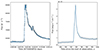 |
Fig. 1. Example of flares detected with the finding algorithm, described in Appendix A.3, shown for TESS (left) and COS (right) observations of Karmn J07446+035 (YZ CMi). The TESS flare, found in Sector 34, the fast (20 s) cadence observation has an ED = 978.54 s and the total energy in TESS bandpass of ≈2.38 × 1033 erg. Applying a correction factor of 0.19 for the TESS CCD response and assuming a blackbody model of 9000 K (Petrucci et al. 2024; Howard & MacGregor 2022) to calculate the bolometric energy of the flare, we obtained Ebol ≈ 1.3 × 1034 erg, consistent with Namizaki et al. (2023). The right panel shows a flare in COS-HST observed 2024-04-12 with starting time 08:36:35.26, with ED = 1836.18 s and a total energy in G130M range of ≈2.70 × 1029 erg. |
To calculate the energy release in the obtained FUV range (106.0–136.0 nm excluding detector gap between 121.0–122.5 nm covering Lyα) for a specific flare event, we used the quiescent surface flux of each flare star calculated from iterative median values of the flux between flare events (i.e. from light curve excluding outliers, as described above). This is expressed as
 (7)
(7)
where Fobs = median(Fobs, ⋆ \ NaN) is the observed de-trended iterative median flux in the span of observation with excluded infinite values, D⋆ is the distance from the Sun, and R⋆ is the star’s radius. Then we can compute
 (8)
(8)
Here, LFUV, ⋆ is the quiescent luminosity in the specific FUV range, Fint, ⋆ is the surface flux, and π ⋅ R⋆2 is the projected disk area of a star.
For our sample stars, we employed the stellar distances most recently reported in the literature and obtained via querying the SIMBAD Astronomical Database (Wenger et al. 2000), as Gaia DR3 does not report distances for numerous targets in our study. The distance values found in the literature for nearby stars up to ∼2 kpc (in case of our sample < 180 pc) exhibit precision comparable to Gaia benchmarks, as demonstrated by cross-validation studies ((Fouesneau et al. 2023, Fig. 7)). Additionally, we derived stellar radii using MIST isochrones, using the TESS T absolute magnitudes. The similar approach was suggested by Howard et al. 2018; Howard & MacGregor 2022. In Feinstein et al. (2022), the authors presented AU Microscopii panchromatic spectra with high resolution. We re-confirmed our approach using this panchromatic flux data for AU Microscopii and compared it with retrieved quiescent spectra values from five different observations of the star by COS-HST. We retrieved the mean value of 1.39 × 1028 erg within the wavelength range of G130M grating (105.815–137.439 nm with covered Lyα), and the quiescent luminosity calculated from panchromatic spectra is similar (1.4 × 1028 erg s−1 according to Feinstein et al. 2022). Therefore, we extended this method for the calculation of quiescent luminosity and released energy in this specific range to the other stars in the sample that have been characterised by FUV observations.
3. Results
3.1. Stellar rotation period analyses
We reported newly determined rotation periods for 119 young stars and the found periods span from 0.14 to 9.75 days. These stars are predominantly members of the β Pictoris and Tucana-Horologium YMGs. While rotation periods can be challenging to measure, particularly with short-baseline data, such as TESS light curves, they are generally reliable for our sample. This is because our dataset is primary composed of young stars exhibiting short rotation periods, and relatively large modulation amplitudes, which are easier to identify and characterize, even within the constraints of TESS observational windows (Shan et al. 2024). Generally, rotation determination is performed using the PDCSAP data from long-duration space missions like Kepler and TESS, and it was our method of choice in this study.
We measured the period of rotation for the sample stars in order to distribute them in period bins in days: Prot < 0.6, 0.6 ≤ Prot < 1.85, 1.85 ≤ Prot < 4, 4 ≤ Prot < 7, 7 ≤ Prot < 30, and Prot ≥ 30. Our bin grid selection aimed to effectively distribute sample stars and isolate very fast rotators in the first bin. We report found periods in the table with the main sample planet parameters available at the CDS. Many stars in the sample already have rotation periods reported in the literature, especially for the CARMENES sample (Shan et al. 2024), and if the found values of rotation period were inside a 10% interval from the literature values, we used our determined periods in subsequent analyses. Our period of rotation calculations sometimes provide different results from TESS and Kepler photometry, which also differ from those found in the literature. In this case, we excluded such stars from the sample. Some of the stars in the sample, whose periods were determined by the periodogram method, would come out with a large discrepancy (> 50% difference in values derived for different sectors or from PDCSAP and SAP data). When such stars had the majority of their detected periods belonging to the same period bin, we included them in the sample and marked them (33 stars total) with a special uncertainty flag. We address the potential explanation of these discrepancies in Sect. 4.
In Fig. 2, we plot the relationship between Hα and log Prot across (G − GRP) colour. In these plots, we distinguish between young stars and field stars (> 800 Myr). The equivalent width of the Hα emission line for the young stars increases with redder values of (G − GRP). The observed variation is primarily attributed to fluctuations in the contribution coming from photosphere, rather than an increase in magnetic activity (Stauffer & Hartmann 1986). Many YMG stars in the colour range corresponding to M dwarfs ∼(G − GRP)≳0.9 exhibit high Hα activity (they fall above the activity boundary line (Kiman et al. 2021), as expected for their young ages (Popinchalk et al. 2021, 2023). The authors of that study did note that this could signal that at the age of Tucana-Horologium, YMG Hα values are independent of the rotation period.
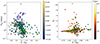 |
Fig. 2. Relationship between Hα and log Prot across (G − GRP) colour from Gaia DR3. Left: Rotation period distribution with (G − GRP) colour-coded by normalised Hα equivalent width. Right: Hα equivalent width against (G − GRP), colour-coded by log Prot. Stars with newly determined periods, Prot, are plotted as circles with lime-green edges, field stars in the sample are represented as circles with blue edges. The M-dwarf activity boundary plotted as a dashed line follows Kiman et al. (2021). |
We observe a subtle correlation where stars with shorter rotation periods and redder (G − GRP) colours tend to exhibit slightly larger Hα equivalent widths; however, curiously, this does not always apply to the fastest rotators (Prot < 0.6). This trend is consistent with the relationship between stellar rotation, colour, and chromospheric activity for young M dwarfs (Skumanich 1972; Mamajek & Hillenbrand 2008). We also comment that the newly determined periods (plotted as circles with lime-green edges) seem to align with the properties of the other young stars in the sample. They exhibit a similar relation between the age and the period and chromospheric activity indicators. The field stars plotted as circles with blue edges exhibit less activity in Hα.
We also examined the rotation period distribution in the context of stellar mass, which we determined based on fitting MIST isochrones to the TESS T absolute magnitudes (see Sect. 2). We binned our sample as follows: M⋆ < 0.11 M⊙, 0.11 M⊙ ≤ M⋆ < 0.3 M⊙, 0.3 M⊙ ≤ M⋆ < 0.45 M⊙, and M⋆ ≥ 0.45 M⊙. We aimed to populate bins effectively, noting that the first two bins likely contain only fully convective stars. The value of the T magnitude for the faintest stars above the values in MIST isochrones for various young ages informed our choice for the right edge of the first bin and we note that sometimes the magnitudes reported in TESS are too faint to correspond to even the smallest mass value for a certain age. This approach enables a distinct analysis of late and mid-late M dwarfs compared to early M and K dwarfs, while maintaining modest-sized sub-samples in each bin.
Another useful parameter for describing stellar magnetic activity-rotation relations is the Rossby number, defined as Ro = Prot/τ, where τ is the convective turnover timescale for a given stellar mass. We calculated it for the stars in the sample from the empirical log τ following Wright et al. (2018). We used these numbers to discuss the implications of measured activity indicators in connection with laws governing frequency flare distributions (see Sect. 4).
3.2. Flare distribution analyses
We analysed flaring activity in the sample stars, following the procedure we described in Appendix A.3. We validated 86 714 flare events with recovery probability > 25%. All events meet our criteria (see Eqs. (A.2), (A.3), (A.4), and (A.5)) and were verified through the injection-recovery procedure, as described in Appendix A.3. The maximum, minimum, and average flare energies detected in the sample are E = 9.23 × 1035 erg, E = 2.87 × 1028 erg, and E = 2.33 × 1032 erg, respectively, which are the TESS flare energies calculated from the observed luminosity of a quiescent star (Kepler flare energies were converted to TESS bandpass using Eq. (A.6)). The individual stars in our sample exhibited from three to 15 969 flare events in the span of observation.
Using the YMDF routines, we look at the flaring rate, the observed energy released in flares, and the power law fit exponent, α, and intercept, β, to the flare frequency distributions (FFDs). These interconnected flare metrics are often used as activity indicators. We proceeded to analyse flare activity by calculating FFDs for each star separately. We plot our resulting FFDs for calculated energies in TESS bandpass released during the flare in Fig. 3 in mass and period bins described above. We provide grey dashed and blue dashed guides corresponding to power law coefficient α = 2.0 and α = 1.5, respectively, for a range of β coefficients. These guide lines facilitate comparison with values for single power law fits found by previous authors. For example, Medina et al. (2020) computed a weighted average of the α = 1.98 ± 0.02 for their sample of mid-to-late M dwarfs. Ilin et al. (2021) investigated K2 light curves of K and M stars and posit that α may be the same for all stars; a value of approximately 2. In the recent study, Feinstein et al. (2024) analysed young stars (ages < 300 Myr) and found α ∼ 1.6 to 1.2 in TESS observations.
The youngest stars in our sample, aged 4.5–5 Myr, exhibit the highest flare energies across all mass ranges. This trend is particularly evident for stars with rotation periods between four and seven days, meaning they are not the fastest rotators, consistent with expectations from being in the disc-locked phase prior to the dissipation of their protoplanetary discs (e.g. Irwin & Bouvier 2009). In contrast, the M dwarfs rotating faster have likely decoupled from their protoplanetary discs due to gas dissipation, enabling faster rotation. The presence or absence of these discs also has implications for ongoing planet formation processes around these young stars.
Stars aged 24–45 Myr populate all bins except the longest period, displaying a shallower slope (α ≈ 1.5) for rotation periods of 1.85–7 days, resulting in a smooth distribution of flare energies. Very low mass stars (M⋆ < 0.11 M⊙) do have rotation periods of less than seven days. These stars and the very fast rotators (Prot < 0.6 days) comprise two populations that exhibit steeper power-law slopes, indicating frequent low-energy flares and rare super-flares, which is evident for young populations and some of the field stars. The picture changes when either the mass or rotation period rises and the population leans towards a power law coefficient of α = 1.5 – up until the point when stars exhibit a rotation period of less than than seven days.
The behaviour of FFDs in the middle part of our grid could reveal the underlying connection between the mass of a star and corresponding period and activity indicators, such as the frequency of small, mid-sized, and extreme flares. The slope α = 1.5 implies that a star would not produce as many small-scale flares as a star that obeys α = 2.0 would. However, there will be a rise in the number of mid-size flares and extreme flares in comparison. With respect to extreme events, it seems that there is no evidence of enhanced super-flare activity in a specific range of M dwarfs with 0.6 ≤ Prot < 7 days and 0.109 M⊙ ≤ M⋆. Moreover, all stars at a certain very-high-energy cut-off will obey the larger slopes. Our results in TESS observations show that both populations in this range, both old and young, show elevated activity in the middle-size flaring compared to α = 2.0. Figure 3 reveals diverse flaring energies among stars with comparable periods and masses. Notably, the FFD slopes of field stars generally align with those of young stars within the same bin.
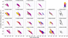 |
Fig. 3. Distribution of the found flare populations in the sample stars in the cumulative form (FFD). The sample is binned in mass and period bins as described in Sect. 3.1. The ages are colour-coded from blue to red to yellow for 4.5–800 Myr; field stars with age > 800 Myr are plotted as grey circles. The grey and blue dashed guides corresponding to power law coefficient α = 2.0 and α = 1.5, respectively, for a range of flare energies ∈[1030, 1036] erg in TESS bandpass. |
From our results, it is apparent that stellar age is not the sole parameter governing flare behaviour. Although Feinstein et al. (2024) found that flare rates are higher when stars are young (less than 50 Myr) and decrease with age, this does not apply to all M dwarfs. For example, the FFD for TRAPPIST-1, the old, low-mass (M⋆ = 0.08 M⊙) and very active M7.5V dwarf (with a value of α = 1.42 computed using MMLE method) show similarities with the FFD for AU Microscopii, a young (belonging to the β Pictoris moving group), more massive (M⋆ = 0.5 M⊙) M0.5-1 pre-main sequence dwarf with power law coefficient of α = 1.46. These stars appear to occupy opposite extremes in stellar properties, yet they exhibit similarly scaled FFDs when normalised to their respective energy regimes. Their derived rotation periods (3.3 days for TRAPPIST-1 and 4.83 days for AU Microscopii in this study) show a close alignment with literature values of 3.304 days (Díez Alonso et al. 2019) and 4.8 days (Yamashita et al. 2024), respectively, and they do not substantially differ from each other either.
We proceeded further with analysing the binned sub-samples using the obtained and corrected equivalent durations of all flare events. As a luminosity-normalised parameter, ED allows for the comparison of flares in different stars, and the simultaneous analysis of flares taking into account the number of stars in sub-samples with different detection thresholds. To do this, we constructed multi-star FFDs by summing the FFDs of all stars belonging to each mass-period bin and normalising the distribution at each ED value by the number of stars that contributed to it. In Fig. 4, we plot the multi-star FFDs for young stars in our sample. Blue dots represent corrected ED and the corrected individual frequencies of each flare by recovery probability. For these multi-star FFDs, we obtained power law coefficients α and intercepts β using the MMLE method as before.
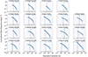 |
Fig. 4. Cumulative distribution plotted for the mass-period bins for young (age < 800 Myr) stars in the sample. Blue dots represent the bin sub-sample FFD, which combines multiple stars by averaging each portion of the FFD by the number of stars that contribute to it. We first calculated initial guess for slope, α1 ini, and intercept, βini, using MMLE method (Maschberger & Kroupa 2009). The initial guess for α2 ini is fixed at 2.0. Then the broken power law was fitted to the distribution, resulting slopes α1, α2 (black dash-dotted lines) and break points (black dashed lines), if the fit was successful. The grey and blue dashed guides corresponding to power law coefficient α = 2.0 and α = 1.5, respectively, plotted for a range of ED ∈ [10−2, 104] days. |
The physical meaning of the FFD power law slope has been discussed previously by several authors. For example, Vida et al. (2017) found α = 1.59 for TRAPPIST-1 and concluded that flare energies of this star are mostly nonthermal and are similar to the energies of other very active M dwarfs found by Hawley et al. (2014). Ilin et al. (2019) noted that flare production is a process with self-similarity in the released energy patterns as it follows a power law; therefore, a deviation from this power law would reflect the underlying physical phenomena. Aschwanden et al. (2016) argued that magnetic and thermal energies dominate around α ∼ 2.0 as opposed to nonthermal energy around α ∼ 1.4. If both thermal and nonthermal processes are in play, it could be interesting to explore the idea that the flare activity will be better represented by the broken power law relation. Based on spotted abrupt changes in power-law slopes in our sample binned for stars’ masses and periods of rotation, we implemented a more sophisticated approach and considered the calculated values of α and the intercept β from MMLE as a first guess for a broken power law routine.
To model the broken power law relationship in our sample FFDs, we employed the BrokenPowerLaw1D class from the Astropy modelling package (Astropy Collaboration 2022). This one-dimensional broken power law model is defined by four key parameters: amplitude A, xbreak, α1, and α2. The amplitude parameter represents the model amplitude at the breakpoint, while xbreak denotes the location of the breakpoint. The model function is mathematically expressed as:
 (9)
(9)
We initialized the BrokenPowerLaw1D model using MMLE-derived α for α1 and 2.0 for α2. We propose that the break likely occurs at EDbreak = 10 s. We then fit this model to our data using Astropy’s LevMarLSQFitter or, if that fails, SimplexLSQFitter. If both fitters end up failing, we then report only the initial power law coefficient estimates. The obtained α1, α2, and breakpoints are given in Fig. 4 and Table 3.
Broken power law coefficients for the mass-period binned sample of young stars.
The young stellar population in our sample generally exhibits initial FFD slopes, α1 ≲ 1.5, except for the lowest-mass stars, which may show slightly larger values. Regarding the second FFD slope, α2, we observe the following trends. The fastest rotators exhibit α2 values closer to 2.0, up to the highest mass bin. In contrast, the remainder of the sample demonstrates substantially shallower slopes. Additionally, the lowest mass bin also shows α2 values approaching 2.0.
We repeated our analysis on the whole sample (i.e. including both young and field stars) to assess how it could affect the slopes of FFDs, as plotted in Fig. B.4. Notwithstanding the evident paucity of slowly rotating young stars, we observed a minimal divergence between the two datasets, with the exception of the scarcely populated (Prot ∈ [1.85, 4] days and M⋆ < 0.11 M⊙) bin, where TRAPPIST-1 flare events cause significant FFD deviation of α2 < 1.5. Field stars generally follow young star behaviour, but while rotating with a period above 30 days, show steep FFD slopes with low-energy flares in this regime. While our sample lacks young stars with Prot > 30 days, the slow-rotating field stars maintain slopes α2 ≥ 2.0, possibly indicating the eventual fate of all M dwarfs at advanced ages, except for the least massive ones. We observe that the highest flare frequency shown in the multi-star FFD exhibits steeper FFD slopes, which correspond to fewer high-energy flares. The young population of the stars in the sample exhibits comparable distribution forms and analogous broken power law coefficients as the whole sample, despite adding the 85 field stars and 35 stars with an age of 800 Myr. Therefore, age does not appear to be an independent factor in determining the flare activity in M dwarfs. The rotational period appears to be a more fundamental indicator of the nuanced FFD behaviour of M dwarfs. Older stars with relatively rapid rotation (e.g. TRAPPIST-1) exhibit the same piecewise and shallower power law as younger stars in the same mass-period bin. Additionally, both fast rotators (< 0.6 days) and slow rotators (≥30 days) tend to have steeper α2 slopes, compared to stars with intermediate rotation periods, regardless of age and up to the highest masses.
The high-energy tails of the FFD deviate from α2 = 2 power law towards steeper values for active stars in our sample, indicating that super-flares are even rarer than previously thought by many authors whose work we mentioned above. These deviations are prominent in all distributions, both for individual stars and the entire sample, as seen in Figs. 3 and 4. We further discussed our findings in Sect. 4.
3.3. Flares in FUV
We analysed flaring activity in the sample stars using the archival observations in FUV for active eleven young stars and six field stars, following the procedure we describe in Sect. 2.4. We found and validated 52 flare events in total (34 and 18 in the young and field stars, respectively). All events met the same criteria as for the TESS/Kepler events (see Eqs. (A.2), (A.3), (A.4), and (A.5)) and were verified through the injection-recovery procedure. The average flare energy detected in the sample is ∼3.5 × 1031 erg, which is the flare energy calculated as EFUV = LFUV, ⋆⋅ ED. We used Eqs. (7) and (8) for the calculation of LFUV, ⋆. These results, along with the summary of the TESS observations for these stars, are presented in Table 4.
UV and white-light activity for several stars in the sample.
Only one star in our small sample of FUV flares, AU Microscopii, has them observed in sufficient amount for frequency analyses. This star exhibited 14 flares with a mean energy of 4.1 × 1029 erg in the specific FUV range during 11.7 hours of observation in total. In Fig. 5, we plotted FFD in FUV flares (the left panel) and in TESS flares (the centre panel) with corresponding broken power law fits and coefficients. We plotted the fitted broken power law slopes, and for the FUV flares, the relations are less steep than for TESS flares; the flares themselves are less energetic and more frequent than those observed in TESS photometry. The high-end tail prominent in TESS FFDs is barely seen in the FUV data, but it can be explained by the lack of super-flares in the observations and the modest size of the sample.
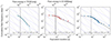 |
Fig. 5. Left and centre panels: Cumulative FFDs (scatter) in ED, and respective broken power law fits (dashed black lines). The y-axis shows the frequency distribution plotted against ED on the x-axis. The secondary x-axis on top represents flare energy. The left panel shows FFD in TESS flares for AU Microscopii. The centre panel represent FFD for FUV flares observed in the same star. Right panel: Cumulative FFDs (scatter) in ED, and respective broken power law fits (dashed black lines) for the sample of FUV flares in young M dwarfs. The y-axis shows the frequency distribution plotted against ED on the x-axis. For all panels, the grey and blue dashed guides corresponding to power law coefficient α = 2.0 and α = 1.5, respectively, for a range of EDs and energies. |
As we obtained the corrected equivalent duration of all flare events in FUV, which allowed us to compare flares in different stars, we proceeded to analyse all FUV sample flares simultaneously. To construct the FFD, we employed the same methodology that incorporates the corrected ED values and the corrected individual frequencies. We applied recovery probability corrections to the individual stars and implemented a weighted averaging approach for each segment of the FFD, where the weighting factor was determined by the number of stars with different detection thresholds contributing to that particular segment. For the young stars in the FUV flare sample, the results are plotted in Fig. 5 (the right panel), and (as done previously for individual FFD for AU Microscopii) we show a fitted broken power law at first slope is even shallower than 1.5 and show good agreement with the slope of 1.58 on the second part. While the 14 flares from AU Microscopii likely dominate the multi-star FFD distribution, it is worth noting that the other two stars, Karmn J07446+035 and 2MASS J02365171-5203036, known as active, each contributed four flares. Importantly, the additional flares in the sample are consistent in terms of ED and released energies, and (more significantly) the fundamental parameters of these stars are somewhat similar. The found relation could hint at differences in energy release in FUV and at visible wavelengths, although for the young stars, it seems that a broken power law with α1 < 1.5 and high energy flares at α2 < 2 is able to accurately represent the flare distribution in both wavelength ranges. We added the six active field stars to the distribution and plotted the results in Fig. B.3. These stars exhibit low to mid-size flares in FUV and including them in the FFD results in an even lower value for α2, along with minimal variations among α1 values.
4. Discussion
4.1. Hα and rotation period as activity indicators
Rotation period determinations typically employ PDCSAP or SAP data analysed with the Lomb-Scargle method, as utilised in this study. This approach, while providing photometry for most of our sample, can encounter challenges when dealing with long rotation periods due to the limited observational windows of TESS. The constraints imposed by TESS’s short-duration observations may lead to uncertainties in accurately identifying extended periodic signals, particularly for slowly rotating stars. We do not report periods longer than ∼10 days, above the problematic periods of 13-14 days often detected in TESS stars. This is due to the TESS mission’s observing strategy: it operates in a lunar-synchronous orbit with a period of 13.7 days, which subjects the telescope to background variations from reflected sunlight, resulting in periodic contamination that is challenging to remove. Therefore, the detection of periods longer than 12–15 days in TESS data presents a challenge (e.g. Avallone et al. 2021; Canto Martins et al. 2020; Holcomb 2020).
In our analysis, we observed a relationship between Hα emission, stellar mass, and age across our sample. We found that the equivalent width of the Hα emission line generally increases with decreasing mass in young stars. This trend is evident in the Hα versus (G − GRP) diagram (see Fig. 2, right panel). The majority of new rotation periods we reported are for stars belonging to the β Pictoris and Tucana-Horologium YMGs, aligning with similar relations observed in previous studies. These findings are consistent with the analysis by Popinchalk et al. (2023), the rotation rate distribution alongside other youth indicators such as Hα of the objects in Tucana-Horologium YMG, which is the second largest sub-group in our sample. They found that the equivalent width of the Hα emission line for their sample increases with decreasing mass at the age of the group due to changes in photospheric contribution and not necessarily more magnetic activity (Kiman et al. 2021). In the Hα against colour-colour diagram, the Tucana-Horologium YMG predominantly occupy a locus typically associated with chromospherically active stellar populations. Popinchalk et al. (2023) conclude that stellar rotation period serves as a robust diagnostic for validating membership in young moving group associations. This conclusion is predicated on the relative ease of measuring rotation periods among young stellar populations.
Overall, YMG stars rarely rotate at a period of less than ∼10 days. In our sample, we have only four stars belonging to the aforementioned groups with greater periods reported in the literature. A distinct transition in the stellar activity that was previously detected in the periods of rotation ∼10 days boundary. This transition was prominent in various observables, including flaring luminosities and amplitudes (Stelzer et al. 2016; Lu et al. 2019). The aforementioned boundary warrants consideration in investigations of field M dwarfs. Our analyses reveal also show the relationship between rotation period and age is clearly non-monotonic. Notably, the youngest stars in our sample exhibit rotation periods of approximately four days, while the older, from 24 to 50 Myr of age, groups include super-fast rotators. Our findings are in agreement with Magaudda et al. (2022) who found that the youngest stars in their sample rotate with periods of ∼4 days. Magaudda et al. (2020) also observed that the X-ray emission level of fast-rotating stars (i.e. those in the saturated regime) is not constant, suggesting the presence of rapid rotators even among older populations, which is in agreement with our results.
The diverse rotational behaviour observed in pre-main sequence stars underscores the complexity of angular momentum evolution in low-mass objects. Our youngest stellar population (4.5–5 Myr) exhibits inflated radii. As young stars contract, the conservation of angular momentum induces spin-up. However, disk-braking mechanisms can counteract this acceleration (Weise et al. 2010). This interplay between contraction-induced spin-up and disk interactions contributes to the intricate rotational evolution observed in young stellar populations, particularly in low-mass stars and brown dwarfs. In the 3-Myr-old Orion Nebula Cluster, Herbst et al. (2002) observed a correlation between stellar rotation rates and infrared excess emission. Specifically, slowly rotating stars exhibited significant infrared excess, indicative of the presence of inner gas disks. Conversely, rapid rotators, characterised by periods shorter than 3.14 days, displayed markedly reduced infrared emission. These findings are aligned with our results and lend support to the hypothesis that protoplanetary disks play a crucial role in modulating stellar angular momentum during the pre-main sequence phase of low-mass stellar evolution (see also e.g. Irwin & Bouvier 2009; Gallet & Bouvier 2015; Reiners & Mohanty 2012).
Another useful parameter for describing stellar magnetic activity-rotation relations is the Rossby number, which is depending on the convective turnover timescale and stellar mass. We calculated it for the stars in the sample from the empirical log τ following Wright et al. (2018). The values of log τ with errors up to ±5% were reported for mass bins in the ranges of ∼0.04–0.19 M⊙. Therefore, it appears unfeasible not to use mass values found using MIST isochrones and the periods reported in this study. For the stars in our sample, the derived Rossby number estimates are expected to be robust.
4.2. The FFD analyses in mass-period bins
In order to construct mass-period bins for our FFDs analyses, we calculated masses for the stars in the sample using TESS T magnitudes and MIST isochrones based on known ages for YMG. However, the isochrone fitting for age determination exhibits significant model-dependent variations. Bell et al. (2015) demonstrated that applying different isochrone models to the β Pic moving group’s observed photometry resulted in age estimates spanning from 10 to 20 Myr. This phenomenon is not isolated to the β Pic group; similar discrepancies have been observed in other nearby moving groups and open clusters (Mamajek & Bell 2014; Kerr et al. 2023; Lee et al. 2024). The disparities in age estimates derived from various isochrones can be attributed to differences in the underlying physics of stellar models, approaches to modelling interior mixing processes, and the stellar atmosphere models employed for bolometric corrections. Moreover, there are known colour discrepancies between observations and model predictions for certain photometry systems and evolutionary stages, which have been discussed in Wang et al. (2025). Since the stellar masses used in this work are primarily for the purpose of assigning stars into coarse bins to study the mass dependence of FFD behaviours, our isochrone-based masses fulfill the precision required. In this case, the faintest stars with uncertainty in the actual mass all fall in the mass bin with M⋆ < 0.11 M⊙ as the approximate upper value for the mass of a star observed with T magnitude larger than the largest available one in the MIST isochrone tables for all age bins for stars in our sample. Given the inherent complexities and potential for introducing additional uncertainties, we have elected to forgo further efforts to refine the mass determinations.
Prevailing models of stellar structure and evolution suggest that stars below ∼0.28–0.35 solar masses maintain fully convective interiors throughout their lifetimes (e.g. Baraffe & Chabrier 2018; Chabrier & Baraffe 1997, 2000). The stars in the two upper rows in the grid shown in Fig. 5 are likely to be fully convective, providing a visual guide that aligns with the physical properties of the stars and enhancing the interpretability of our mass- and rotation period-based binning strategy.
The lowest-mass bin for stars with M⋆ < 0.11 M⊙ shows the tendency to obey α2 ∼ 2.0 and steeper in the high-energy tail, while the more massive stars FFDs depart to lower values of α even at the larger energy cut-offs or larger ED. In several previous studies (Howard et al. 2019; Ilin et al. 2019, 2021), the large α ∼ 2.0 coefficients were spotted for stars of different ages given that the authors use high energy cut-off for fitting power laws or subsequent analyses, as in Medina et al. (2020). Analysing the FFDs in young stars in a wide variety of spectral types, Feinstein et al. (2024) found that in their sample, the young stars obey α = 1.5. Our results show that only the fast-rotating very-low-mass stars in our sample (whatever the age) show either a quick switch to α2 ∼ 2.0 regime or the massive high-energy tail is sometimes even steeper than that. However, for higher masses or rotation periods, the population tends towards a power law coefficient α2 ≃ 1.5–1.7, until stars with Prot ≥ 30 days again exhibit a tendency to follow a power law with larger α2. Notably, all individual stellar FFDs with sufficient flare counts exhibit a distinct break in their power-law slopes (see e.g. Fig. 5, left panel for AU Microscopii). This observation naturally leads to the idea of a piecewise power law, which was not previously fully implemented in the studies of FFDs in young and active M dwarfs.
4.3. The FFDs in young dwarfs are governed by piecewise power law
The observed FFDs in mass-period bins deviate from a single power law at lower energies, which cannot be fully explained by detection limitations. While distance can affect flare detection in general (i.e. for the distant stars the detection will be only available for the most energetic events), for stars within 200 pc (which is primary zone for TESS survey), other factors such as stellar type, intrinsic flare energy, and observational cadence are likely to have a more significant impact on the detectable flare distribution than distance alone. Hawley et al. (2014) demonstrated that even flares with durations of 10 minutes (corresponding to amplitude 0.002 and log EKp ∼ 30.5) are readily identifiable in Kepler data with 1 minute cadence, suggesting that a significant number of such flares is likely being detected, rather than going unnoticed. TESS’s overall sensitivity to weak flares remains somewhat lower than that of Kepler, despite this enhanced temporal resolution (Tu et al. 2020; Doyle et al. 2019). Nevertheless, the inclusion of fast-cadence (20 s) TESS light curves for numerous stars in our sample, combined with the injection-recovery routine (see Appendix A.3 for details), significantly enhanced our ability to reliably detect and validate smaller flare events.
The deviation from a single power law may indicate that lower energy flares follow a different power law distribution compared to high energy flares, as discussed by Hannah et al. (2011) for solar flares. Wheatland (2010) presented evidence suggesting a deviation from the power-law distribution in flare sizes for a small solar active region and suggested a piecewise Poisson distribution, correlating with the evolving magnetic topology of the region under observation. Paudel et al. (2018) found deviations from a single power-law dependence for some targets in their small sample of ultra-cool dwarfs. Studying active and inactive M dwarfs in Kepler data, Hawley et al. (2014) conducted analyses that indicate that the power-law fit does not persist at lower energies, even though they lie above the detection limit. They surmised that this discrepancy may arise from either the incorporation of low-energy flares into complex events or a genuine turnover in the power-law distribution.
Observed flare events may actually be composite phenomena comprising multiple concurrent flares of varying energies. The apparent break in the power law distribution may stem from the challenge of distinguishing overlapping low-energy flares, which are often classified as single, more energetic events. This issue is exacerbated by the lack of spatial resolution in Kepler and TESS data. While resolving these complex flare structures might yield a distribution closer to a simple power-law, our current observational constraints necessitate the use of a broken power-law model, as it may more accurately represent the true flare energy distribution, accounting for both physical differences in flare generation mechanisms and observational limitations. This approach provides a more realistic representation of stellar activity, crucial for studies of exoplanet atmospheres.
4.4. Activity patterns
The observed patterns in FFDs within our parameter space probe the intrinsic relationships among stellar mass, rotation period, and various activity indicators. These indicators include the occurrence rates of small-scale, moderate, and extreme flaring events. The broken power law approach will allow us to accurately describe small-scale and mid-size flares, which is applicable in flare models to study the radiative environment for the planetary systems of M dwarfs. As for the super-flare events, they require special consideration, as our analysis indicates that such events are exceedingly rare – sometimes even rarer than suggested by a power law with α ∼ 2.0 – regardless of the age, mass, or rotation period observed in M dwarfs, and even for the youngest and most active stars these events’ frequency will fall short of the slope of α ∼ 1.5.
As reported in Popinchalk et al. (2023) in their evaluation of activity patterns for M dwarfs belonging to Tucana-Horologium, for 0.6 < (G − GRP) < 1.2, the Hα values are independent of rotation period. The Rossby number, which combines rotation period and convective turnover time, is a key indicator of stellar magnetic activity, and its activity relation evolves with stellar age. It was therefore of interest to investigate whether the Hα activity indicator could signal changes in the FFDs of young stars. In Fig. B.5, we plotted the logarithm of the Rossby number for our mass-period bins in the sample against the Hα equivalent width (EW Hα). The relationship between age and EW Hα is apparent, with the largest values of EW Hα corresponding to the youngest stars. However, the previously observed nuanced relationship between rotation periods and FFDs behaviour does not seem to manifest itself distinctly in the EW Hα measurements. Overall, we observe a large variation in the behaviour of the stars’ activity, even for stars with nominally similar properties.
4.5. Comparing scalar flare rate across stellar properties
Since observable flares occur with a wide range of energies for a given star, such a frequency can be seen as for flares of a given energy or larger (e.g. ten flares per year with E ≥ 1032 erg). This is equivalent to evaluating the FFD at a given energy. The specific flare rate has been used in some capacity for many years for comparing flare activity levels between stars and was noted by Davenport (2016) as an effective metric for comparing flare activity levels between stars at different distances. Medina et al. (2020) selected a threshold flare energy of 3.16 × 1031 ergs (log10(E) = 31.5) in the TESS bandpass for their sample of low mass stars at distances less than 15 pc. This threshold was chosen by the authors because it corresponds to the energy at which the completeness function reaches or exceeds 50% for all stars in their sample of M and L dwarfs and ensured a consistent level of flare detection completeness across our entire stellar sample in the TESS observations.
The YMGs to which the stars in our sample of M-K dwarfs belong are at mean distances from 29 to 172 pc and brighter than TESS magnitude 14. We determined that the mean energy of the photometric flares in our sample is 1.9 × 1032 ergs. This average energy is higher than the aforementioned threshold and could potentially be attributed to the heightened activity levels characteristic of young stars and aligns with the expectation that younger stellar populations exhibit more energetic flaring events, reflecting their enhanced magnetic activity. It was established that rapidly rotating stars tend to show more flares, but the highest flare rates are not necessarily found among the fastest rotators (Raetz et al. 2020). The youngest population of stars in our sample do indeed exhibit energetically highest flares, while their rotation periods put them in Prot ∈ [4, 7] days bin.
In Fig. 6, we plot the fitted relations for four mass bins used in our study, with coloured lines representing different period bins. We propose that these relations can be applied in modelling the distribution and evolution of flaring activity of young stars with corresponding stellar properties, in conjunction with their rotation histories. This approach would enable more precise assessments of the radiative environment in evolutionary models of planet-star interactions. Such a refinement could significantly enhance our understanding of how stellar activity impacts planetary evolution in young stellar systems.
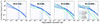 |
Fig. 6. Broken power law relation for FFDs found in this study sample of young and field stars is plotted for four mass bins. The colour of the lines indicates the period bins. The lines represent the broken power law slopes α1 and α2 for successful fits. Uncertainties are plotted as light envelopes in the same colour as period bins. |
4.6. Evaluating UV FFD behaviour in YMG members
In this study, we utilised archival FUV observations of low-mass stars to evaluate the UV predictions of existing FFDs for photometry observations. We employed HST TIME-TAG spectroscopy to produce time-resolved light curves and further implement our flare finding and injection-recovery routines. In Fig. 5 we present the resulting FFD for one star, AU Microscopii, in the optical range (left panel) and FUV (centre panel), along with the multi-star sample FFD in UV (right panel). The UV flare distribution demonstrates a broken power law with α2 = 1.48, while the TESS observations show much steeper α2 = 1.8. It could indicate the different flare frequency behaviour in the different wavelength ranges. However, Tristan et al. (2023), studied the multi-wavelength activity of AU Microscopii in NUV photometry and soft X-ray, finding that both wavelength range distributions show similarity in α ∼ 1.72; this result is slightly shallower, compared to our results in TESS bandpass for the same star. For FUV activity in AU Microscopii, we found a much shallower second slope. The discrepancies may be attributed to the incompleteness of our sample or variations in the FFD behaviour across different regions of the spectrum.
Studying NUV flare energies and frequencies, Paudel et al. (2024) and Rekhi et al. (2023) found that the flares in this range are much more frequent in comparison to optical. For the FUV range, Jackman et al. (2024) reports a higher frequency of ultraviolet flares exhibiting minimal or undetectable corresponding optical signatures. Analysis of HST COS FUV data revealed power-law coefficients of 1.58 for flare energies and 1.61 for EDs in M-type stars belonging to the Tucana-Horologium YMG ((Loyd et al. 2020, Fig. 1)). Although the authors’ analysis is based on a limited sample of 18 flares, the α values they report are consistent with our results when considering α2 alone, as identifying a broken power-law becomes difficult with small sample sizes. For the field stars, they found enhanced α coefficients of 1.74 and 1.77 for energy and ED, respectively. However, incorporating older stars in our multi-star FFD analysis (Fig. B.3) yielded an even lower α2 = 1.39, for which our larger sample size could be the explanation. Our results suggest that flares with longer EDs are more frequently detected in the FUV, compared to the visible wavelengths for a given star. The same tendency is apparent in the multi-star analyses (Fig. 5, right panel). This disparity warrants further investigation into the underlying physics of stellar flare generation across different spectral ranges and implies that the processes driving flare occurrence may differ between FUV and visible emissions, particularly in young stellar objects.
Loyd et al. (2020) detected FUV flares from the optically quiet stars, while Jackman et al. (2024) found that various models, for instance, a 9000 K blackbody, the combination of it and the Great AD Leo flare characterisation by Hawley & Pettersen (1991), and Fiducial flare model proposed by Loyd et al. (2018a) significantly underestimate emission across all ages, masses, and activity levels. These discrepancies reach up to four orders of magnitude for combined FUV continuum and line emission. The authors noted that underestimation is even greater for individual emission lines, highlighting the need for improved modelling approaches to accurately represent stellar emission processes. This suggests that the spectral energy distribution in flares varies between the partially convective and fully convective interiors. This could also suggest that the transition to a fully convective interior alters the underlying magnetic field generation mechanisms, leading to variations in energy fractionation across all wavelengths. Jackman et al. (2024) also worked with the Tucana-Horologium YMG to investigate potential age-dependent changes in flare model accuracy. By comparing UV correction factors between the 40 Myr sample and field age stars within the same mass range, they identified that models underestimate FUV emission less severely as stars get on in age.
Our sample of the UV flares is small and relatively incomplete compared to the extensive photometric flare dataset, which enabled more in-depth analyses. However, in this small sample, we spotted the power law for the second slope of α2 = 1.58, which is similar to found by Feinstein et al. (2022) for the stars belonging to YMG (α ∼ 1.5 − 1.6). Concurrently, the entire sample of young and field stars of UV flares, examined in this study and plotted in Fig. B.3, displays shallow slopes. While our UV sample size is not sufficient for definitive conclusions, the observed discrepancy in flare frequency behaviour for AU Microscopii and presumably for many young stars as seen in Fig. 5 suggests potentially distinct flare production in the UV and visible wavelength regimes and shows some support to the broken power law model for flare energy distributions. We note that in their work, Tristan et al. (2023) demonstrates that the FFDs of AU Microscopii, along with those of the reference stars YY Gem and Proxima Centauri, could plausibly be characterised by a piecewise power-law model (their Fig. 10).
The FUV regime enables detection of lower-energy flares through direct observation of chromospheric activity, whereas optical wavelengths predominantly reveal high-energy white-light events requiring photospheric heating. To be detectable in the TESS bandpass, flares must inject sufficient energy to heat the photosphere, resulting in reduced observational sensitivity to low-energy white-light events. This is supported by multiple detections of UV flares with non-detectable or weakly detectable optical counterparts (Jackman et al. 2024; Brasseur et al. 2023; Paudel et al. 2024; Rekhi et al. 2023). Consequently, the FUV regime exhibits enhanced detectability of lower energy flare events compared to optical observations. The alignment between the FUV’s α2 slope and the low-energy optical regime’s α1 slope likely arises because FUV observations probe the low-energy FFD and the lack of high-energy events in our sample of UV flares reflects the limited observational baselines of COS/HST data (typically hours per target compared to TESS’s 27-day continuous monitoring per sector). Future studies incorporating additional simultaneous optical, NUV, FUV, and X-ray observations will enable better constraints on the relative occurrence of flares across these wavelength regimes for low-mass stars.
5. Conclusions
Our investigation into flare activity in young M dwarfs, particularly those in YMGs, has yielded crucial insights into their stellar flare behaviour with the potential impact on atmospheres of exoplanets around them. We demonstrate that stellar rotation period and mass serve as fundamental parameters governing flare frequency distributions (more so than age alone), suggesting more complex mechanisms govern frequency-flare distributions than previously hypothesised.
We propose a novel approach using a piece-wise power law model for low-to-mid-size and large flares in young M dwarfs, allowing for a more nuanced representation of flare behaviour across energy ranges. This method, combined with known rotation periods, enables the generation of more realistic flare event sequences, which are crucial for assessing exoplanet atmosphere stability and potential habitability. While the conflation of large and small flares does not significantly impact the total energy budget, it can lead to atypical power-law relationships. Observational biases at distribution extremes must be considered when interpreting stellar activity patterns and their implications for exoplanetary environments. Our broken power law approach in FFDs can improve the modelling of activity patterns in specific young M dwarfs.
These findings have significant implications for future exoplanet characterisation missions, particularly those studying M dwarf terrestrial planet atmospheres. By providing a more accurate picture of the flare environment, we can better predict challenges inherent in detecting biosignatures and assessing habitability.
Data availability
The dataset comprising stellar parameters obtained in this study are available at the CDS via anonymous ftp to cdsarc.cds.unistra.fr (130.79.128.5) or via https://cdsarc.cds.unistra.fr/viz-bin/cat/J/A+A/700/A53
Acknowledgments
We acknowledge financial support from the Research Council of Norway (RCN), through its Centres of Excellence funding scheme, projects number 332523 (PHAB, Centre for Planetary Habitability) and number 262622 (ROCS, Rosseland Centre for Solar Physics). We thank Konstantin Herbst (PHAB), Alexey Pankine (Space Science Institute, USA) and Adalyn Gibson (University of Colorado Boulder, USA) for the fruitful discussion. We thank the anonymous reviewer for the thoughtful feedback that helped to improve this manuscript.
References
- Aigrain, S., Parviainen, H., & Pope, B. J. S. 2016, MNRAS, 459, 2408 [NASA ADS] [Google Scholar]
- Aschwanden, M. J., Holman, G., O’Flannagain, A., et al. 2016, ApJ, 832, 27 [Google Scholar]
- Astropy Collaboration (Price-Whelan, A. M., et al.) 2022, ApJ, 935, 167 [NASA ADS] [CrossRef] [Google Scholar]
- Avallone, E. A., Tayar, J., Van Saders, J., Berger, T., & Claytor, Z. 2021, Am. Astron. Soc. Meeting Abstr., 238, 314.07 [Google Scholar]
- Baraffe, I., & Chabrier, G. 2018, A&A, 619, A177 [NASA ADS] [CrossRef] [EDP Sciences] [Google Scholar]
- Bell, C. P. M., Mamajek, E. E., & Naylor, T. 2015, MNRAS, 454, 593 [Google Scholar]
- Bloomfield, D. S., Mathioudakis, M., Christian, D. J., Keenan, F. P., & Linsky, J. L. 2002, A&A, 390, 219 [NASA ADS] [CrossRef] [EDP Sciences] [Google Scholar]
- Bonfils, X., Lo Curto, G., Correia, A. C. M., et al. 2013, A&A, 556, A110 [NASA ADS] [CrossRef] [EDP Sciences] [Google Scholar]
- Borucki, W. J., Koch, D., Basri, G., et al. 2010, Science, 327, 977 [Google Scholar]
- Brasseur, C. E., Osten, R. A., Tristan, I. I., & Kowalski, A. F. 2023, ApJ, 944, 5 [Google Scholar]
- Caldwell, D. A., Tenenbaum, P., Twicken, J. D., et al. 2020, Res. Notes Am. Astron. Soc., 4, 201 [Google Scholar]
- Canto Martins, B. L., Gomes, R. L., Messias, Y. S., et al. 2020, ApJS, 250, 20 [NASA ADS] [CrossRef] [Google Scholar]
- Chabrier, G., & Baraffe, I. 1997, A&A, 327, 1039 [NASA ADS] [Google Scholar]
- Chabrier, G., & Baraffe, I. 2000, ARA&A, 38, 337 [Google Scholar]
- Chang, S. W., Byun, Y. I., & Hartman, J. D. 2015, ApJ, 814, 35 [NASA ADS] [CrossRef] [Google Scholar]
- Christian, D. J., Mathioudakis, M., Bloomfield, D. S., et al. 2006, A&A, 454, 889 [NASA ADS] [CrossRef] [EDP Sciences] [Google Scholar]
- Creevey, O. L., Sordo, R., Pailler, F., et al. 2023, A&A, 674, A26 [NASA ADS] [CrossRef] [EDP Sciences] [Google Scholar]
- Cui, K., Liu, J., Yang, S., et al. 2019, MNRAS, 489, 5513 [NASA ADS] [CrossRef] [Google Scholar]
- Cully, S. L., Siegmund, O. H. W., Vedder, P. W., & Vallerga, J. V. 1993, ApJ, 414, L49 [Google Scholar]
- Davenport, J. R. A. 2016, ApJ, 829, 23 [Google Scholar]
- Davenport, J. R. A., Hawley, S. L., Hebb, L., et al. 2014, ApJ, 797, 122 [Google Scholar]
- Díez Alonso, E., Caballero, J. A., Montes, D., et al. 2019, A&A, 621, A126 [NASA ADS] [CrossRef] [EDP Sciences] [Google Scholar]
- Dotter, A. 2016, ApJS, 222, 8 [Google Scholar]
- Doyle, L., Ramsay, G., Doyle, J. G., & Wu, K. 2019, MNRAS, 489, 437 [Google Scholar]
- Dressing, C. D., & Charbonneau, D. 2015, ApJ, 807, 45 [Google Scholar]
- Dupree, A. K., Lobel, A., Young, P. R., et al. 2005, ApJ, 622, 629 [Google Scholar]
- Engle, S. G. 2024, ApJ, 960, 62 [NASA ADS] [CrossRef] [Google Scholar]
- Feinstein, A. D., France, K., Youngblood, A., et al. 2022, AJ, 164, 110 [NASA ADS] [CrossRef] [Google Scholar]
- Feinstein, A. D., Seligman, D. Z., France, K., Gagné, J., & Kowalski, A. 2024, AJ, 168, 60 [Google Scholar]
- Fouesneau, M., Frémat, Y., Andrae, R., et al. 2023, A&A, 674, A28 [NASA ADS] [CrossRef] [EDP Sciences] [Google Scholar]
- France, K., Linsky, J. L., Tian, F., Froning, C. S., & Roberge, A. 2012, ApJ, 750, L32 [Google Scholar]
- Frasca, A., Biazzo, K., Lanzafame, A. C., et al. 2015, A&A, 575, A4 [NASA ADS] [CrossRef] [EDP Sciences] [Google Scholar]
- Froning, C. S., Kowalski, A., France, K., et al. 2019, ApJ, 871, L26 [NASA ADS] [CrossRef] [Google Scholar]
- Gagné, J., & Faherty, J. K. 2018, ApJ, 862, 138 [Google Scholar]
- Gaia Collaboration (Vallenari, A., et al.) 2023, A&A, 674, A1 [NASA ADS] [CrossRef] [EDP Sciences] [Google Scholar]
- Gaidos, E., & Mann, A. W. 2013, ApJ, 762, 41 [Google Scholar]
- Gallet, F., & Bouvier, J. 2015, A&A, 577, A98 [NASA ADS] [CrossRef] [EDP Sciences] [Google Scholar]
- Gershberg, R. E. 1972, Ap&SS, 19, 75 [Google Scholar]
- Hannah, I. G., Hudson, H. S., Battaglia, M., et al. 2011, Space Sci. Rev., 159, 263 [NASA ADS] [CrossRef] [Google Scholar]
- Hawley, S. L., & Fisher, G. H. 1992, ApJS, 78, 565 [NASA ADS] [CrossRef] [Google Scholar]
- Hawley, S. L., & Pettersen, B. R. 1991, ApJ, 378, 725 [Google Scholar]
- Hawley, S. L., Fisher, G. H., Simon, T., et al. 1995, ApJ, 453, 464 [NASA ADS] [CrossRef] [Google Scholar]
- Hawley, S. L., Davenport, J. R. A., Kowalski, A. F., et al. 2014, ApJ, 797, 121 [Google Scholar]
- Herbst, W., Bailer-Jones, C. A. L., Mundt, R., Meisenheimer, K., & Wackermann, R. 2002, A&A, 396, 513 [EDP Sciences] [Google Scholar]
- Hilton, E. J., West, A. A., Hawley, S. L., & Kowalski, A. F. 2010, AJ, 140, 1402 [Google Scholar]
- Hirschauer, A. S. 2023, COS Instrument Handbook, 16, 16 [Google Scholar]
- Holcomb, R. 2020, Am. Astron. Soc. Meeting Abstr., 235, 274.04 [Google Scholar]
- Howard, W. S., & MacGregor, M. A. 2022, ApJ, 926, 204 [NASA ADS] [CrossRef] [Google Scholar]
- Howard, W. S., Tilley, M. A., Corbett, H., et al. 2018, ApJ, 860, L30 [Google Scholar]
- Howard, W. S., Corbett, H., Law, N. M., et al. 2019, ApJ, 881, 9 [NASA ADS] [CrossRef] [Google Scholar]
- Howell, S. B., Sobeck, C., Haas, M., et al. 2014, PASP, 126, 398 [Google Scholar]
- Hunt-Walker, N. M., Hilton, E. J., Kowalski, A. F., Hawley, S. L., & Matthews, J. M. 2012, PASP, 124, 545 [NASA ADS] [CrossRef] [Google Scholar]
- Ilin, E., Schmidt, S. J., Davenport, J. R. A., & Strassmeier, K. G. 2019, A&A, 622, A133 [NASA ADS] [CrossRef] [EDP Sciences] [Google Scholar]
- Ilin, E., Schmidt, S. J., Poppenhäger, K., et al. 2021, A&A, 645, A42 [NASA ADS] [CrossRef] [EDP Sciences] [Google Scholar]
- Ilin, E., Schmidt, S. J., Poppenhäger, K., et al. 2022, AltaiPony: Flare finder for Kepler, K2, and TESS light curves, Astrophysics Source Code Library [record ascl:2201.009] [Google Scholar]
- Irwin, J., & Bouvier, J. 2009, in The Ages of Stars, eds. E. E. Mamajek, D. R. Soderblom, & R. F. G. Wyse, IAU Symp., 258, 363 [Google Scholar]
- Jackman, J. A. G., Shkolnik, E. L., Loyd, R. O. P., & Richey-Yowell, T. 2024, MNRAS, 533, 1894 [Google Scholar]
- Jenkins, J. M., Caldwell, D. A., Gilliland, R. L., et al. 2010, AAS/Division for Planetary Sciences Meeting Abstracts, 42, 27.09 [Google Scholar]
- Jenkins, J. M., Twicken, J. D., McCauliff, S., et al. 2016, in Software and Cyberinfrastructure for Astronomy IV, eds. G. Chiozzi, & J. C. Guzman, SPIE Conf. Ser., 9913, 99133E [Google Scholar]
- Kerr, R. M. P., Rizzuto, A. C., Kraus, A. L., & Offner, S. S. R. 2021, ApJ, 917, 23 [NASA ADS] [CrossRef] [Google Scholar]
- Kerr, R., Kraus, A. L., & Rizzuto, A. C. 2023, ApJ, 954, 134 [Google Scholar]
- Kiman, R., Faherty, J. K., Cruz, K. L., et al. 2021, AJ, 161, 277 [NASA ADS] [CrossRef] [Google Scholar]
- Kowalski, A. F., Hawley, S. L., Wisniewski, J. P., et al. 2013, ApJS, 207, 15 [NASA ADS] [CrossRef] [Google Scholar]
- Kowalski, A. F., Wisniewski, J. P., Hawley, S. L., et al. 2019, ApJ, 871, 167 [CrossRef] [Google Scholar]
- Kraus, A. L., Shkolnik, E. L., Allers, K. N., & Liu, M. C. 2014, AJ, 147, 146 [Google Scholar]
- Lammer, H., Lichtenegger, H. I. M., Kulikov, Y. N., et al. 2007, Astrobiology, 7, 185 [NASA ADS] [CrossRef] [Google Scholar]
- Lee, R. A., Gaidos, E., van Saders, J., Feiden, G. A., & Gagné, J. 2024, MNRAS, 528, 4760 [NASA ADS] [CrossRef] [Google Scholar]
- Lightkurve Collaboration (Cardoso, J. V. D. M., et al.) 2018, Lightkurve: Kepler and TESS time series analysis in Python, Astrophysics Source Code Library [record ascl:1812.013] [Google Scholar]
- Lomb, N. R. 1976, Ap&SS, 39, 447 [Google Scholar]
- Loyd, R. O. P., France, K., Youngblood, A., et al. 2018a, ApJ, 867, 71 [Google Scholar]
- Loyd, R. O. P., Shkolnik, E. L., Schneider, A. C., et al. 2018b, ApJ, 867, 70 [NASA ADS] [CrossRef] [Google Scholar]
- Loyd, R. O. P., Shkolnik, E. L., France, K., Wood, B. E., & Youngblood, A. 2020, Res. Notes Am. Astron. Soc., 4, 119 [Google Scholar]
- Lu, H.-P., Zhang, L.-Y., Shi, J., et al. 2019, ApJS, 243, 28 [NASA ADS] [CrossRef] [Google Scholar]
- Luhman, K. L. 2007, ApJS, 173, 104 [Google Scholar]
- Lurie, J. C., Davenport, J. R. A., Hawley, S. L., et al. 2015, ApJ, 800, 95 [Google Scholar]
- Magaudda, E., Stelzer, B., Covey, K. R., et al. 2020, A&A, 638, A20 [NASA ADS] [CrossRef] [EDP Sciences] [Google Scholar]
- Magaudda, E., Stelzer, B., Raetz, S., et al. 2022, A&A, 661, A29 [NASA ADS] [CrossRef] [EDP Sciences] [Google Scholar]
- Malo, L., Doyon, R., Lafrenière, D., et al. 2013, ApJ, 762, 88 [Google Scholar]
- Mamajek, E. E., & Bell, C. P. M. 2014, MNRAS, 445, 2169 [Google Scholar]
- Mamajek, E. E., & Hillenbrand, L. A. 2008, ApJ, 687, 1264 [Google Scholar]
- Mamonova, E., Shan, Y., Hatalova, P., & Werner, S. C. 2024, A&A, 685, A143 [NASA ADS] [CrossRef] [EDP Sciences] [Google Scholar]
- Maschberger, T., & Kroupa, P. 2009, MNRAS, 395, 931 [NASA ADS] [CrossRef] [Google Scholar]
- Medina, A. A., Winters, J. G., Irwin, J. M., & Charbonneau, D. 2020, ApJ, 905, 107 [Google Scholar]
- Namizaki, K., Namekata, K., Maehara, H., et al. 2023, ApJ, 945, 61 [NASA ADS] [CrossRef] [Google Scholar]
- Narain, U., & Ulmschneider, P. 1996, Space Sci. Rev., 75, 453 [Google Scholar]
- Owen, T. 1980, in The Search for Early Forms of Life in Other Planetary Systems: Future Possibilities Afforded by Spectroscopic Techniques, ed. M. D. Papagiannis (Dordrecht: Springer, Netherlands), 177 [Google Scholar]
- Paudel, R. R., Gizis, J. E., Mullan, D. J., et al. 2018, ApJ, 858, 55 [Google Scholar]
- Paudel, R. R., Barclay, T., Youngblood, A., et al. 2024, ApJ, 971, 24 [Google Scholar]
- Paxton, B., Smolec, R., Schwab, J., et al. 2019, ApJS, 243, 10 [Google Scholar]
- Petrucci, R. P., Gómez Maqueo Chew, Y., Jofré, E., Segura, A., & Ferrero, L. V. 2024, MNRAS, 527, 8290 [Google Scholar]
- Pineda, J. S., Youngblood, A., & France, K. 2021, ApJ, 911, 111 [NASA ADS] [CrossRef] [Google Scholar]
- Popinchalk, M., Faherty, J. K., Kiman, R., et al. 2021, ApJ, 916, 77 [NASA ADS] [CrossRef] [Google Scholar]
- Popinchalk, M., Faherty, J. K., Curtis, J. L., et al. 2023, ApJ, 945, 114 [NASA ADS] [CrossRef] [Google Scholar]
- Raetz, S., Stelzer, B., Damasso, M., & Scholz, A. 2020, A&A, 637, A22 [NASA ADS] [CrossRef] [EDP Sciences] [Google Scholar]
- Ranjan, S., Wordsworth, R., & Sasselov, D. D. 2017, ApJ, 843, 110 [Google Scholar]
- Redfield, S., Linsky, J. L., Ake, T. B., et al. 2002, ApJ, 581, 626 [Google Scholar]
- Reiners, A., & Mohanty, S. 2012, ApJ, 746, 43 [Google Scholar]
- Rekhi, P., Ben-Ami, S., Perdelwitz, V., & Shvartzvald, Y. 2023, ApJ, 955, 24 [Google Scholar]
- Ricker, G. R. 2016, in AGU Fall Meeting Abstracts, P13C-01 [Google Scholar]
- Ricker, G. R., Winn, J. N., Vanderspek, R., et al. 2015, J. Astron. Telescopes Instrum. Syst., 1, 014003 [Google Scholar]
- Savitzky, A., & Golay, M. J. E. 1964, Anal. Chem., 36, 1627 [Google Scholar]
- Scargle, J. D. 1982, ApJ, 263, 835 [Google Scholar]
- Schneider, A. C., Shkolnik, E. L., Allers, K. N., et al. 2019, AJ, 157, 234 [Google Scholar]
- Segura, A., Walkowicz, L. M., Meadows, V., Kasting, J., & Hawley, S. 2010, Astrobiology, 10, 751 [Google Scholar]
- Seli, B., Vida, K., Moór, A., Pál, A., & Oláh, K. 2021, A&A, 650, A138 [NASA ADS] [CrossRef] [EDP Sciences] [Google Scholar]
- Shan, Y., Yee, J. C., Bowler, B. P., et al. 2017, ApJ, 846, 93 [NASA ADS] [CrossRef] [Google Scholar]
- Shan, Y., Revilla, D., Skrzypinski, S. L., et al. 2024, A&A, 684, A9 [NASA ADS] [CrossRef] [EDP Sciences] [Google Scholar]
- Shibayama, T., Maehara, H., Notsu, S., et al. 2013, ApJS, 209, 5 [Google Scholar]
- Skumanich, A. 1972, ApJ, 171, 565 [Google Scholar]
- Stassun, K. G., Oelkers, R. J., Paegert, M., et al. 2019, AJ, 158, 138 [Google Scholar]
- Stauffer, J. R., & Hartmann, L. W. 1986, ApJS, 61, 531 [NASA ADS] [CrossRef] [Google Scholar]
- Stelzer, B., Damasso, M., Scholz, A., & Matt, S. P. 2016, MNRAS, 463, 1844 [NASA ADS] [CrossRef] [Google Scholar]
- Thompson, S. E., Fraquelli, D., Van Cleve, J. E., & Caldwell, D. A. 2016, in Kepler Archive Manual, Kepler Science Document KDMC-10008-006, eds. F. Abney, D. Sanderfer, M. R. Haas, & S. B. Howell, 9 [Google Scholar]
- Tilley, M. A., Segura, A., Meadows, V., Hawley, S., & Davenport, J. 2019, Astrobiology, 19, 64 [Google Scholar]
- Torres, G., Andersen, J., & Giménez, A. 2010, A&A Rev., 18, 67 [Google Scholar]
- Tovar Mendoza, G., Davenport, J. R. A., Agol, E., Jackman, J. A. G., & Hawley, S. L. 2022, AJ, 164, 17 [CrossRef] [Google Scholar]
- Tristan, I. I., Notsu, Y., Kowalski, A. F., et al. 2023, ApJ, 951, 33 [NASA ADS] [CrossRef] [Google Scholar]
- Tu, Z.-L., Yang, M., Zhang, Z. J., & Wang, F. Y. 2020, ApJ, 890, 46 [NASA ADS] [CrossRef] [Google Scholar]
- Van Cleve, J. E., & Caldwell, D. A. 2016, in Kepler Instrument Handbook, Kepler Science Document KSCI-19033-002, eds. M. R. Haas, & S. B. Howell, 1 [Google Scholar]
- VanderPlas, J. T. 2018, ApJS, 236, 16 [Google Scholar]
- Venot, O., Rocchetto, M., Carl, S., Roshni Hashim, A., & Decin, L. 2016, ApJ, 830, 77 [NASA ADS] [CrossRef] [Google Scholar]
- Vida, K., Kővári, Z., Pál, A., Oláh, K., & Kriskovics, L. 2017, ApJ, 841, 124 [Google Scholar]
- Wang, F., Fang, M., Fu, X., et al. 2025, ApJ, 979, 92 [Google Scholar]
- Weise, P., Launhardt, R., Setiawan, J., & Henning, T. 2010, A&A, 517, A88 [NASA ADS] [CrossRef] [EDP Sciences] [Google Scholar]
- Wenger, M., Ochsenbein, F., Egret, D., et al. 2000, A&AS, 143, 9 [NASA ADS] [CrossRef] [EDP Sciences] [Google Scholar]
- Wheatland, M. S. 2004, ApJ, 609, 1134 [CrossRef] [Google Scholar]
- Wheatland, M. S. 2010, ApJ, 710, 1324 [Google Scholar]
- Wood, B. E., Müller, H.-R., Redfield, S., et al. 2021, ApJ, 915, 37 [NASA ADS] [CrossRef] [Google Scholar]
- Wright, N. J., Newton, E. R., Williams, P. K. G., Drake, J. J., & Yadav, R. K. 2018, MNRAS, 479, 2351 [Google Scholar]
- Yamashita, M., Itoh, Y., & Takagi, Y. 2024, A&A, 691, A304 [NASA ADS] [CrossRef] [EDP Sciences] [Google Scholar]
- Zuckerman, B. 2019, ApJ, 870, 27 [Google Scholar]
Appendix A: Detailed methodology
A.1. Hα emission data and analyses
The intrinsic faintness of M dwarfs has made the Hα line the primary diagnostic spectral feature of chromospheric activity. For stars in the sample, we retrieved Hα emission detection, using the literature (specifically, the EW Hα values come from Kraus et al. (2014) for Tucana-Horologium YMG, from Frasca et al. (2015) for Chamaeleon I YMG and from Schneider et al. (2019) for β Pictoris YMG) and the Gaia DR3 dataset. From the latter, we obtained a Hα pseudo-equivalent width (pEW) computed as the integrated normalised flux over a wavelength domain (646-670 nm, i.e. at both sides of 656.5 nm). Measuring the Hα emission line presents significant challenges, particularly for stars with temperatures below 4000 K. These difficulties arise from two main factors: the limited resolving power of BP and RP spectra, and the sharp decrease in transmission efficiency at the Hα wavelength, and the issue is thoroughly discussed in Fouesneau et al. (2023). To address the spectral complexity in cooler stars and mitigate blending effects with non-hydrogen species, the authors implemented a correction strategy. They subtracted the equivalent width derived from the nearest synthetic spectrum below 5000 K within the GSP-Phot atmospheric parameter space (denoted as EW, Hα, model).
 (A.1)
(A.1)
We proceeded to compare the Hα pseudo-equivalent width measured by Extended Stellar Parametrizer for Emission-Line Stars (ESP-ELS), a module within the Gaia astrophysical parameters inference system (Apsis, used in Gaia DR3, Creevey et al. 2023) to the published equivalent width values. In Fig. A.1, left panel, we plot the age of young stars in our sample against EW Hα, both including and excluding EW, Hα, model (note that our sample does not contain stars with Teff > 5000 K). In the same figure, in the left panel, we plotted the relation for EW Hα reported in the literature and EW Hα from ESP-ELS. Including and excluding the model would not lead to the agreement with literature, while including the model results in underestimating the Hα strength, and excluding it leads to overestimating EW Hα for the stars of the age 24-800 Myr. For very young stars, represented in our sample by two groups of 4.5-5 Myr, the data in the literature are scarce. Despite the Gaia pEW Hα values for the youngest stars showing disagreement with the literature in some cases, we consider pEW Hα from Gaia in the form recommended by Eq. A.1 as the estimate of the Hα line strength for the youngest stars in our sample due the absence of these EW Hα values in literature.
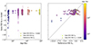 |
Fig. A.1. Comparison of EW Hα from Gaia DR3 and literature. Left panel: For the sample of stars, three values of equivalent width of Balmer α line were plotted according to Eq.A.1: Gaia DR3 EW Hα, Gaia DR3 EW Hα with added model and EW Hα found in literature. Right panel: the diagram presents the effect of the model from the relation described in Eq.A.1. Ages of the sample’s stars are colour-coded from youngest (blue) to oldest (yellow). |
For analyses of the activity of stars in our sample, we used the Rossby number, the indicator that connects such parameters as mass and period of rotation. The values of log τ were reported for mass bins with errors up to ±5% of the value. Therefore, it seems impractical not to use mass values found using MIST isochrones and the found periods because most of the sample stars showed rotation periods within error intervals of the values reported previously or did not differ from them more than 10%. The uncertainties in M⋆ and Prot propagate into our Rossby number calculations. We utilise log τ values from Wright et al. (2018), reported with ±5% uncertainty, which aligns well with our mass bins derived from MIST isochrone-based M⋆ estimates. The additional source of uncertainty in Ro stems from Prot. For most stars, our derived Prot values align well with previous reports, typically well within 10%. Consequently, we estimate the typical uncertainty in Ro to be approximately 10%, primarily driven by the combined uncertainties in τ and Prot and does not compromise the reliability of the calculated Rossby number estimates.
A.2. Light curve data processing
The stars’ sample analysed in this study was observed by both the Kepler and TESS missions. For Kepler light curve data, we used the Kepler Science Processing Pipeline (Jenkins et al. 2010), which processes science data collected from the Kepler Photometer: raw and systematic error corrected flux time series. For K2 data, we used K2 pipeline (Thompson et al. 2016) produced light curve files by using simple aperture photometry. For TESS we used the TESS Science Processing Operations Center (SPOC) pipeline (Caldwell et al. 2020), which generates and calibrates target light curves.
From the MAST, we downloaded processed data from both long cadence (LC), 1800 s, and short cadence (SC), 60 s, star light curves from Kepler (Jenkins et al. 2010), LC 1800 s and SC 60 s cadence data from K2 (Howell et al. 2014), following the LC (1800 s/600 s/200 s) and SC data (120 s/ 20 s) from TESS missions (Jenkins et al. 2016). We downloaded light curves, corrected the detection efficiency, and proceeded to de-trend and remove the variability. We used the light curves first for the period of rotation determination. For several stars, we reported new periods, in other cases, we used values we found if they were within ±10% of those found in literature, and if we were unable to find or determine the rotation period, the star was excluded from the sample.
Utilising the light curve data described above, we derived stellar rotation periods from photometric modulations caused by rotating starspots. These variations typically occur on longer timescales compared to flare events. For stars in the sample, we started with downloading LC TESS data, which is available at 1800 s intervals for TESS Cycles 1 and 2 (sectors 1-26), the 600 s cadence data in Cycles 3 and 4 (sectors 27-55), and the 200 sec data in Cycles 5 and 6 (sectors 56-83). We continue by downloading all available 90-day LC quarters and sectors of Kepler and K2 for our sample. Kepler has been observing stars at 29.4-minute intervals as LC targets for the primary purpose of detecting transiting planets. For determination of the rotation period and hereafter we used Lightkurve module (Lightkurve Collaboration 2018).
A.3. Flare detection
To be able to work simultaneously with light curves from TESS and Kepler and collected data from the UV instrument COS on board HST, we implemented the YMDF Python routine based on the Python module ‘altaipony‘ (Ilin et al. 2021, 2022), which was designed for finding and analysing flares in Kepler, K2, and TESS photometry. The ‘altaipony‘ module uses the Automated flare finding routine Appaloosa, the open-source flare finding and analysis procedure written in Python by Davenport (2016) for Kepler and the algorithm, designed by Aigrain et al. (2016) for de-trending and variability removal, hereafter ‘autofinder‘. The module also uses ‘lightKurve‘ Python package for downloading the data. For the de-trending of data, we apply a Savitky-Golay filter (Savitzky & Golay 1964) to the light curve. The filter is based on the method of data smoothing by local least-squares polynomial approximation, and it works by fitting a polynomial to a small window of adjacent data points and using this polynomial to estimate the value of the central point in the window. The window is then shifted along the signal, and the process is repeated for each point in the signal. The de-trending of the light curve allows us to flag outliers, and they were clipped at 3σ iteratively. This method was chosen by Ilin et al. (2021) because it is sufficiently quick and provides satisfying results in both Kepler and TESS light curves. At the next step, for the detection of flare events, we used the following conditions: the flare candidate definition follows the criteria in Chang et al. (2015):
 (A.2)
(A.2)
 (A.3)
(A.3)
 (A.4)
(A.4)
 (A.5)
(A.5)
where xi is the current flux value,  and σL are the local mean and standard deviation for a given light curve, wi is the photometric error at epoch i, and ConM is the number of consecutive points which satisfy Eq.A.2, A.3, and A.4. The values of N1, N2, and N3 are taken to be 3, 3, and 2, respectively (the recommended values according to Chang et al. 2015; Ilin et al. 2022). This model simplifies the task of detecting significant statistical outliers and can identify flare candidates with 3σ above the iterative median flux, regardless of intrinsic variability.
There are several effects the flare finding algorithm can produce: large flares may appear larger, and small flare candidates may be unaccounted for. The former occurs when stellar variability adds flux to the flare, which was mitigated by de-trending preprocessing. The latter arises when small flares in the de-trended light curve fail to meet the criteria distinguishing them from quiescent flux. To account for these effects, we applied an injection-recovery routine, comparing recovered events to injected ones. Following Davenport et al. (2014), who suggest a piecewise model for flare shapes, our module produced and injected an array of artificial flares constructed following the flare model in Tovar Mendoza et al. (2022) into every light curve where at least one flare event was observed.
The flare recovery completeness has also been computed throughout each light curve, where we found the flare activity using artificial flare injection tests, and we used the tools and the empirical flare model, first suggested by Davenport (2016) and implemented in the YMDF module. The artificial events were introduced to each light curve at randomly generated times with varying amplitude and duration while avoiding overlap with real flare signatures. A flare was then considered recovered if the flare peak time was contained within the start and end times of any resulting flare event candidate. After relating all successful and failed detections to each other, the recovery rate as a function of equivalent duration was returned. The method for calculating the probability of recovering tiles up the sample of artificial flares into amplitude and duration bins twice: first, it tiles up the sample into a matrix based on the recovered amplitude and durations, second, it does the same with the injected flare parameters, and so include also those injected flares that were not recovered. The first matrix is used to map each flare candidate’s recovered equivalent duration to a value that accounts for losses dealt to the equivalent duration by photometric noise and introduced by the de-trending procedure. The typical injected amplitude and duration of flares in that tile of the matrix can then be used by the second matrix to derive the candidate’s recovery probability from the ratio of lost to recovered injected flares.
A.4. White-light flare analysis
Using the formalism from Sect. 2.3 (Eqs. 1, 2, 3, and 4), we calculated the energy of every flare exhibited by stars in our sample. For these calculations, we obtained the Kepler instrument response function for low resolution from the Kepler Instrument Handbook (Van Cleve & Caldwell 2016), and the TESS response function5. We note that by this approximation we miss at least the ∼27% of the continuum flare flux that resides in the U band relative to the total in UBVR (Hawley & Fisher 1992) and flux from emission lines that lie outside the Kepler band (Kowalski et al. 2013). As a consequence, EKp, flare should be considered a lower limit to the total released energy of the flare (Ilin et al. 2019).
Vida et al. (2017) showed that the flare energies from Kepler can be converted to flare energies in the TESS bandpass as follows:
 (A.6)
(A.6)
This results in a 0.14 shift on the logarithmic energy scale. While working with our sample from both Kepler and TESS missions, we recalculated found values of energy in the TESS bandpass, as the majority of our sample stars’ light curves originated from TESS survey.
The ’mcmc’ model was considered preferable by the aforementioned authors, and they follow Wheatland (2004, Eq. 24) using the Markov chain Monte Carlo method (MCMC), and sampling from the joint posterior distribution with a constant prior. For quicker results, we used the modified maximum likelihood estimator (MMLE), which is detailed in Maschberger & Kroupa (2009), to find the slope α. The least squares method was used to fit to estimate the intercept β. Having established a common value of α, we can fix this value to estimate the flare rate for stars with fewer than five flares, and to obtain a more precise value of the flare rate for stars with five or more flares. This simplified approach is sufficient as the resulting values only serve as an initial estimate for assessing the power law distributions in the flare sample. We proceed with these calculations for all stars in the sample.
In the previous studies (Howard et al. 2019; Chang et al. 2015; Medina et al. 2020; Gaidos & Mann 2013; Raetz et al. 2020), the ED, energy or duration cut-off is usually introduced for power law coefficients calculation. We quantified the completeness in our study of FFD: to assess the effectiveness of the aforementioned ’autofinder’ algorithm, we conducted a completeness study. The corrections to the number and energy of detected flare events are based on two factors: the detection probability and the energy recovery ratio. For every flare in the sample, we retrieved the recovery probability Prec and used only flares with Prec > 0.25 instead of cutting off the flares that cannot be considered super-flares. We did that because we are interested also in the middle-range energy flares, as they comprise the majority of young M dwarfs’ flares and it can potentially largely affect exoplanets’ atmospheres.
A.5. HST/COS flare analyses
We retrieved archival data from the HST COS G130M grating, identified by program IDs: 14784 (PI Shkolnik); 15071, 16033 (PI Froning); 16482 (PI Roman-Duval); 15955 (PI Richey-Yowell); 16164 (PI Cauley); 17428 (PI France); 11533 (PI Green). This grating is centered at 122.2 nm, with resolving power R = λ/Δλ∼12 000-16 000, following the configuration used in Froning et al. (2019), Feinstein et al. (2022). This setup offers spectral coverage spanning approximately 106.0–136.0 nm, with a detector gap between 121.0–122.5 nm. This gap strategically masks the intense Lyα emission feature to avoid detector saturation. The same COS setting was used for all analyses. We selected this specific grating based on two key considerations. Firstly, it provides coverage of chromospheric and transition region emission lines, which are crucial for investigating far-ultraviolet (FUV) emission and activity in low-mass stars. Secondly, the abundance of observations available using this grating enables us to maintain self-consistency throughout our study, enhancing the reliability and comparability of our results across multiple targets.
For TIME-TAG mode observations, CALCOS creates a corrected events list (i. e. "corrtag" file) that preserves the time-stamped photon events. To create time-resolved flux data from COS observations using the G130M grating, we extracted spectra from the corrtag file. Each extraction involved selecting events within the specified time range, applying wavelength calibration, and converting counts to flux using the appropriate sensitivity curve. For the data reduction, we binned the observations into 20 s exposures to balance high temporal cadence with a sufficiently high signal-to-noise ratio (S/N) per bin, as previous studies (i.e. Howard & MacGregor 2022) suggest that the time resolution can impact measured flare amplitudes and energies.
The initial AltaiPony package, on which we are based our YMDF routine, was made to work with high quality, uniformly processed final data from these TESS and Kepler surveys (i.e. PDS-SAP fluxes), that is, with already removed instrumental and astrophysical variability for the signal. In the case of COS-HST data reduction, the CALCOS pipeline, as previously described, corrects the data for instrumental effects, including noise, thermal drifts, geometric distortions, and pixel-to-pixel sensitivity variations, generates an exposure-specific wavelength-calibrated scale, and extracts and produces the final one-dimensional, flux-calibrated, time-resolved spectrum. We, therefore, implemented the same framework in the YMDF, including routines: i) de-trending flux; ii) find, characterise, inject and recover flare events; iii) calculating corrected EDs (in seconds) and recovery probability; to work with time-resolved flux integrated across FUVB-FUVA range for 20 s exposure time steps.
Appendix B: Supplementary tables and figures
Broken power law coefficient for the mass-period binned sample of young and field stars.
 |
Fig. B.1. Example of a light curve (left), a periodogram (centre) and a folded light curve (right) for UCAC4 208-001676 in TESS Sector 1 with the fitted frequency of 1.03 days found by the Lomb-Scargle method. At the centre panel, the period at maximum power, found by the periodogram method, is clearly seen as a peak value. We analysed four sectors of TESS data for this star: 2, 3, 29, 30, 69 and the average period found to be 1.02 days. |
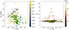 |
Fig. B.2. Plot of the relationship between Hα from Gaia DR3 including the model (see Eq. A.1) and logProt across (G - GRP)) colour from Gaia DR3, presented as a compliment our analyses in discrepancies between EW Hα measured by ESP-ELS in Gaia DR3 and the values reported in literature. Left: Rotation period distribution with (G - GRP)) colour-coded by normalised Hα equivalent width. Right: Hα equivalent width against (G - GRP), colour-coded by logProt. Stars with newly determined periods Prot are plotted as circles with lime-green edges, field stars in the sample are represented as circles with blue edges. The M-dwarf activity boundary plotted as dashed line follows Kiman et al. (2021) |
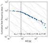 |
Fig. B.3. Cumulative FFDs (scatter) in ED, and respective broken power law fits (dashed black lines) for the sample of FUV flares in young and field stars in this study sample. The y-axis shows the frequency distribution plotted against ED on the x-axis. The grey and blue dashed guides corresponding to power law coefficient α = 2.0 and α = 1.5, respectively, for a range of ED. |
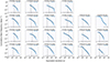 |
Fig. B.4. Cumulative distribution for the mass-period bins of all stars in this study sample. Blue dots represent the bin sub-sample FFD, which takes to account multiple stars by averaging each portion of the FFD by the number of stars that contribute to it. Initial guess for slope α1 ini and intercept βini from MMLE method as before were used to fit the broken power law was to the distribution resulting slopes α1, α2 (black dash-dotted lines) and break points indicated by black dashed lines, if the fit was successful. The grey and blue dashed guides corresponding to power law coefficient α = 2.0 and α = 1.5, respectively, are plotted for a range of ED ∈[10−2, 104] days. |
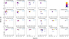 |
Fig. B.5. Relation between the Rossby number and EW Hα. The dots are colour-coded according to the age of the star. Initial guess for slope αini along with the broken power law slopes α1 and α2 for successful fits are stated for every mass-period bin. |
All Tables
Broken power law coefficient for the mass-period binned sample of young and field stars.
All Figures
|
Fig. 1. Example of flares detected with the finding algorithm, described in Appendix A.3, shown for TESS (left) and COS (right) observations of Karmn J07446+035 (YZ CMi). The TESS flare, found in Sector 34, the fast (20 s) cadence observation has an ED = 978.54 s and the total energy in TESS bandpass of ≈2.38 × 1033 erg. Applying a correction factor of 0.19 for the TESS CCD response and assuming a blackbody model of 9000 K (Petrucci et al. 2024; Howard & MacGregor 2022) to calculate the bolometric energy of the flare, we obtained Ebol ≈ 1.3 × 1034 erg, consistent with Namizaki et al. (2023). The right panel shows a flare in COS-HST observed 2024-04-12 with starting time 08:36:35.26, with ED = 1836.18 s and a total energy in G130M range of ≈2.70 × 1029 erg. |
| In the text | |
|
Fig. 2. Relationship between Hα and log Prot across (G − GRP) colour from Gaia DR3. Left: Rotation period distribution with (G − GRP) colour-coded by normalised Hα equivalent width. Right: Hα equivalent width against (G − GRP), colour-coded by log Prot. Stars with newly determined periods, Prot, are plotted as circles with lime-green edges, field stars in the sample are represented as circles with blue edges. The M-dwarf activity boundary plotted as a dashed line follows Kiman et al. (2021). |
| In the text | |
|
Fig. 3. Distribution of the found flare populations in the sample stars in the cumulative form (FFD). The sample is binned in mass and period bins as described in Sect. 3.1. The ages are colour-coded from blue to red to yellow for 4.5–800 Myr; field stars with age > 800 Myr are plotted as grey circles. The grey and blue dashed guides corresponding to power law coefficient α = 2.0 and α = 1.5, respectively, for a range of flare energies ∈[1030, 1036] erg in TESS bandpass. |
| In the text | |
|
Fig. 4. Cumulative distribution plotted for the mass-period bins for young (age < 800 Myr) stars in the sample. Blue dots represent the bin sub-sample FFD, which combines multiple stars by averaging each portion of the FFD by the number of stars that contribute to it. We first calculated initial guess for slope, α1 ini, and intercept, βini, using MMLE method (Maschberger & Kroupa 2009). The initial guess for α2 ini is fixed at 2.0. Then the broken power law was fitted to the distribution, resulting slopes α1, α2 (black dash-dotted lines) and break points (black dashed lines), if the fit was successful. The grey and blue dashed guides corresponding to power law coefficient α = 2.0 and α = 1.5, respectively, plotted for a range of ED ∈ [10−2, 104] days. |
| In the text | |
|
Fig. 5. Left and centre panels: Cumulative FFDs (scatter) in ED, and respective broken power law fits (dashed black lines). The y-axis shows the frequency distribution plotted against ED on the x-axis. The secondary x-axis on top represents flare energy. The left panel shows FFD in TESS flares for AU Microscopii. The centre panel represent FFD for FUV flares observed in the same star. Right panel: Cumulative FFDs (scatter) in ED, and respective broken power law fits (dashed black lines) for the sample of FUV flares in young M dwarfs. The y-axis shows the frequency distribution plotted against ED on the x-axis. For all panels, the grey and blue dashed guides corresponding to power law coefficient α = 2.0 and α = 1.5, respectively, for a range of EDs and energies. |
| In the text | |
|
Fig. 6. Broken power law relation for FFDs found in this study sample of young and field stars is plotted for four mass bins. The colour of the lines indicates the period bins. The lines represent the broken power law slopes α1 and α2 for successful fits. Uncertainties are plotted as light envelopes in the same colour as period bins. |
| In the text | |
|
Fig. A.1. Comparison of EW Hα from Gaia DR3 and literature. Left panel: For the sample of stars, three values of equivalent width of Balmer α line were plotted according to Eq.A.1: Gaia DR3 EW Hα, Gaia DR3 EW Hα with added model and EW Hα found in literature. Right panel: the diagram presents the effect of the model from the relation described in Eq.A.1. Ages of the sample’s stars are colour-coded from youngest (blue) to oldest (yellow). |
| In the text | |
|
Fig. B.1. Example of a light curve (left), a periodogram (centre) and a folded light curve (right) for UCAC4 208-001676 in TESS Sector 1 with the fitted frequency of 1.03 days found by the Lomb-Scargle method. At the centre panel, the period at maximum power, found by the periodogram method, is clearly seen as a peak value. We analysed four sectors of TESS data for this star: 2, 3, 29, 30, 69 and the average period found to be 1.02 days. |
| In the text | |
|
Fig. B.2. Plot of the relationship between Hα from Gaia DR3 including the model (see Eq. A.1) and logProt across (G - GRP)) colour from Gaia DR3, presented as a compliment our analyses in discrepancies between EW Hα measured by ESP-ELS in Gaia DR3 and the values reported in literature. Left: Rotation period distribution with (G - GRP)) colour-coded by normalised Hα equivalent width. Right: Hα equivalent width against (G - GRP), colour-coded by logProt. Stars with newly determined periods Prot are plotted as circles with lime-green edges, field stars in the sample are represented as circles with blue edges. The M-dwarf activity boundary plotted as dashed line follows Kiman et al. (2021) |
| In the text | |
|
Fig. B.3. Cumulative FFDs (scatter) in ED, and respective broken power law fits (dashed black lines) for the sample of FUV flares in young and field stars in this study sample. The y-axis shows the frequency distribution plotted against ED on the x-axis. The grey and blue dashed guides corresponding to power law coefficient α = 2.0 and α = 1.5, respectively, for a range of ED. |
| In the text | |
|
Fig. B.4. Cumulative distribution for the mass-period bins of all stars in this study sample. Blue dots represent the bin sub-sample FFD, which takes to account multiple stars by averaging each portion of the FFD by the number of stars that contribute to it. Initial guess for slope α1 ini and intercept βini from MMLE method as before were used to fit the broken power law was to the distribution resulting slopes α1, α2 (black dash-dotted lines) and break points indicated by black dashed lines, if the fit was successful. The grey and blue dashed guides corresponding to power law coefficient α = 2.0 and α = 1.5, respectively, are plotted for a range of ED ∈[10−2, 104] days. |
| In the text | |
|
Fig. B.5. Relation between the Rossby number and EW Hα. The dots are colour-coded according to the age of the star. Initial guess for slope αini along with the broken power law slopes α1 and α2 for successful fits are stated for every mass-period bin. |
| In the text | |
Current usage metrics show cumulative count of Article Views (full-text article views including HTML views, PDF and ePub downloads, according to the available data) and Abstracts Views on Vision4Press platform.
Data correspond to usage on the plateform after 2015. The current usage metrics is available 48-96 hours after online publication and is updated daily on week days.
Initial download of the metrics may take a while.