| Issue |
A&A
Volume 700, August 2025
|
|
|---|---|---|
| Article Number | A82 | |
| Number of page(s) | 18 | |
| Section | Planets, planetary systems, and small bodies | |
| DOI | https://doi.org/10.1051/0004-6361/202554623 | |
| Published online | 07 August 2025 | |
Resurgence of CO in a warm bubble around accreting protoplanets and its observability
1
Charles University, Faculty of Mathematics and Physics, Astronomical Institute,
V Holešovičkách 747/2,
180 00 Prague 8,
Czech Republic
2
Departamento de Astronomía, Universidad de Chile,
Casilla 36-D,
Santiago,
Chile
3
Data Observatory Foundation,
Eliodoro Yáñez 2990,
Providencia,
Santiago,
Chile
★ Corresponding author: This email address is being protected from spambots. You need JavaScript enabled to view it.
Received:
18
March
2025
Accepted:
23
June
2025
Abstract
The cold outer regions of protoplanetary disks are expected to contain a midplane-centered layer where gas-phase CO molecules freeze out and their overall abundance is low. The layer then manifests itself as a void in the channel maps of CO rotational emission lines. We explore whether the frozen-out layer can expose the circumplanetary environment of embedded accreting protoplanets to observations. To this end, we performed 3D radiative gas-dust hydrodynamic simulations with opacities determined by the redistribution of submicron- and millimeter-sized dust grains. A Jupiter-mass planet with an accretion luminosity of ∼ 10−3 L☉ was considered as the nominal case. The accretion heating sustains a warm bubble around the planet, which locally increases the abundance of gas-phase CO molecules. Radiative transfer predictions of the emergent sky images show that the bubble becomes a conspicuous CO emission source in channel maps. It appears as a low-intensity optically thick spot located in between the so-called dragonfly wings that trace the fore-and backside line-forming surfaces. The emission intensity of the bubble is nearly independent of the tracing isotopolog, suggesting a very rich observable chemistry, as long as its signal can be deblended from the extended disk emission. This can be achieved with isotopologs that are optically thin or weakly thermally stratified across the planet-induced gap, such as C18O. For these, the bubble stands out as the brightest residual in synthetic ALMA observations after subtraction of axially averaged channel maps inferred from the disk kinematics, enabling new automatic detections of forming protoplanets. By contrast, the horseshoe flow steadily depletes large dust grains from the circumplanetary environment, which becomes unobservable in the submillimeter continuum, in accordance with the scarcity of ALMA detections.
Key words: hydrodynamics / radiative transfer / planets and satellites: detection / planets and satellites: formation protoplanetary disks / planet-disk interactions
© The Authors 2025
 Open Access article, published by EDP Sciences, under the terms of the Creative Commons Attribution License (https://creativecommons.org/licenses/by/4.0), which permits unrestricted use, distribution, and reproduction in any medium, provided the original work is properly cited.
This article is published in open access under the Subscribe to Open model. This email address is being protected from spambots. You need JavaScript enabled to view it. to support open access publication.
1 Introduction
A wealth of substructures discovered in the outer regions1 of protoplanetary disks (see Andrews 2020; Bae et al. 2023; Benisty et al. 2023, and references therein) poses a challenge for the theory of planet formation. The question is whether some of these substructures can indirectly trace embedded protoplanets that perturb their natal disk. For instance, protoplanets that become massive enough to modify the rotation curve of the surrounding gas can induce pressure barriers for drifting dust grains that result in dusty rings (e.g. Paardekooper & Mellema 2006; Zhu et al. 2012; Dipierro et al. 2016; Zhang et al. 2018; Lodato et al. 2019). However, pressure barriers can also form by multiple processes that are not related to the presence of protoplanets (for reviews see Pinilla & Youdin 2017; Bae et al. 2023). Observations of substructures are therefore typically not sufficient to decide whether protoplanets are present. Supporting evidence is needed.
To date, direct detections of protoplanets have been rare. Several candidates were identified through high-contrast near-infrared imaging (Keppler et al. 2018; Currie et al. 2022; Hammond et al. 2023; Wagner et al. 2023; Christiaens et al. 2024). Of these sources, only PDS 70 b and c and AB Aur b exhibit detectable H α emission (Wagner et al. 2018; Haffert et al. 2019; Zhou et al. 2021, 2025), which provides evidence for ongoing gas accretion onto hypothetic giant protoplanets. Finally, only PDS 70 c can be detected in the submillimeter (submm) continuum (Isella et al. 2019; Benisty et al. 2021), which indicates a dusty circumplanetary disk (CPD) or free-free emission that is driven by gas accretion (given the variability of the signal; Casassus & Cárcamo 2022). The scarcity of ALMA (Atacama Large Millimeter/submillimeter Array) continuum detections of CPDs contrasts with existing predictions from isothermal and nonisothermal simulations (e.g. Wolf & D’Angelo 2005; Szulágyi et al. 2018) or steady-state analytical models (Zhu et al. 2018), which suggest the formation of a conspicuous and bright CPD in the continuum.
The disk kinematics inferred from submm molecular line emission provide a promising way of detecting protoplanets. Planet-induced perturbations modify the trajectories of gas parcels and their respective line-of-sight velocities compared to a disk in pure sub-Keplerian rotation. If the deviations become strong enough, wiggles or kinks can appear in the channel maps (Perez et al. 2015; Pinte et al. 2018b, 2019), which are most commonly obtained for CO isotopologs. This kinematic analysis can also be performed based on the velocity centroid maps. The idea is to subtract the axially symmetric background flow and isolate the velocity reversal in the planet-induced spiral wakes (Pérez et al. 2018; Casassus & Pérez 2019; Chen & Dong 2024).
Large-scale kinematic features are generated at line-forming surfaces at altitudes of up to a few scale heights (e.g. Law et al. 2022), offset from the midplane-positioned protoplanets themselves. While these features are relatively ubiquitous in 12CO, however, they are surprisingly less pronounced in rarer isotopologs that probe deeper disk layers (Pérez et al. 2020), and their origin cannot be uniquely attributed to a specific body (e.g. the case of AS 209; Bae et al. 2022; Fedele et al. 2023). Interestingly, the models that yield submm-bright CPDs also predict bright molecular line emission that is expected to persist in multiple channels (Perez et al. 2015). Nevertheless, the line persistence effect has not yet been convincingly detected (except possibly in AS 209 and Elias 2-24; Bae et al. 2022; Pinte et al. 2023).
Here, we examine the tension between the observed wealth of structure in disks and the scarcity of radio-continuum protoplanet detections, and we consider whether the accretion luminosity of an embedded protoplanet can facilitate a detectable and rich chemistry of the circumplanetary environment regardless of the formation of a CPD (see also Cleeves et al. 2015; Jiang et al. 2023; Petrovic et al. 2024). We use the fact that outside the CO snowline2, the gas-phase molecules of CO freeze out and become depleted in an interior layer of the disk. Consequently, for moderately inclined disks, the fore- and backside ‘dragonfly wings’ that appear in channel maps become separated by a void from which CO is absent (for similar considerations, see Dullemond et al. 2020). We envisage that if the accreting luminous protoplanet orbits within the CO-depleted layer, it heats up the surrounding gas (Benítez-Llambay et al. 2015; Montesinos et al. 2015; Szulágyi 2017; Muley et al. 2024) and prevents freeze-out locally, which means that the abundance of CO molecules is higher than in the cold surroundings. When the resulting CO bubble that encapsulates the planet is observed at a convenient viewing geometry, it might be localized within the emission void and might also be isolated as a kinematic signal.
To provide a proof of concept, we performed 3D dust-gas radiation hydrodynamic simulations of disk-embedded luminous protoplanets, converted the result into synthetic images, and searched for observable features. Important aspects of our modeling involved the direct treatment of heating and cooling processes, which is essential to avoid ambiguity between the temperature profile and the dynamical state of the gas, and direct tracking of millimeter-sized (mm-sized) dust grains, which allowed us to predict the thermal continuum emission together with the molecular line emission. Our hydrodynamic and radiative transfer methods are described in Sect. 2. A nominal simulation, described in Sect. 3, serves as a case study in conditions whose observability is discussed in Sect. 4. The supporting analysis of the nominal simulation is provided in Appendix A, and additional configurations are documented in Appendix B. We discuss our findings and conclude in Sect. 5.
2 Methods
2.1 Equations of 3D two-fluid radiation hydrodynamics
We modeled a 3D protoplanetary disk on an Eulerian mesh in spherical coordinates (radius r, azimuth φ, and colatitude θ). The disk comprised three components: gas, large dust grains (with a physical size  mm), and small dust grains (
 μm). The two-population dust model follows the reasoning of Ziampras et al. (2025) and allowed us to (i) study the effect of the redistribution of large grains on the thermal properties of the disk, (ii) predict dust continuum observations, and (iii) account for dust coagulation at least in a simple parametric manner. To do this, we introduced a coagulation parameter that sets the initial solid mass fraction contained in mm-sized grains,
 (1)
(1)
where  and
and  are the surface densities of large and small dust grains, respectively3.
The population of small grains was strongly aerodynamically coupled with the gas. We assumed that the coupling was ideal so that the small grains behaved as tracers of the gas distribution and did not have to be evolved explicitly. The volume density of small dust grains  can be derived from the gas density ρg at any time using
 (2)
(2)
where  is the initial dust-to-gas ratio.
To model the coupled evolution of gas and large grains, we adopted a pressureless fluid approximation for the latter and solved the following equations of two-fluid hydrodynamics:
 (3)
(3)
 (4)
(4)
 (5)
(5)
 (6)
(6)
where we introduced the gas velocity v, the pressure P, the viscous stress tensor T, the gravitational potential Φ, the aerodynamic drag acceleration adrag, the dust velocity u, and the turbulent dust diffusion flux j.
The equation of state was that of an ideal gas,
 (7)
(7)
where γ=1.43 is the adiabatic index, ε is the internal energy density of gas, cV is the heat capacity at constant volume, and T is the temperature. We assumed that the gas and dust grains were thermalized and therefore described by the same T.
The kinematic gas viscosity was parameterized following Shakura & Sunyaev (1973),
 (8)
(8)
with α=5 × 10⁻⁴, cs being the sound speed, and ΩK being the Keplerian orbital frequency. The viscosity enters the calculation through tensor T (for a full definition of T, see Benítez-Llambay & Masset 2016), and because it is thought to be driven by unresolved underlying turbulence, we assumed that it sets the level of dust diffusion as well (Morfill & Voelk 1984),
 (9)
(9)
The gravitational potential reads
![Mathematical equation: $\Phi=-\frac{G M_{\star}}{r}-\frac{G M_{\mathrm{p}}}{d}\left[\left(\frac{d}{r_{\mathrm{sm}}}\right)^{4}-2\left(\frac{d}{r_{\mathrm{sm}}}\right)^{3}+2 \frac{d}{r_{\mathrm{sm}}}\right],$](/articles/aa/full_html/2025/08/aa54623-25/aa54623-25-eq16.png) (10)
(10)
where G is the gravitational constant, M★ is the mass of the central star, Mp is the planet mass, d is the cell-planet distance, and rsm is the smoothing length. The potential of an embedded planet (the last term in Eq. (10)) was smoothed with a cubic spline as in Klahr & Kley (2006).
The aerodynamic drag was considered as a two-way acceleration (it appears with opposite signs in Eqs. (4) and (6)) to preserve momentum conservation and was defined as
 (11)
(11)
where St is the Stokes number (the dimensionless stopping time) of large dust grains. In our model, the Stokes number was set to vary from one cell to the next according to
 (12)
(12)
where ρmat is the material density of large grains. We capped the Stokes number as St ≤0.5, however, in order to ensure that (i) the Schmidt number4 remained ≈1 (which is implicitly assumed in writing Eq. (9)) and (ii) the fluid approximation for dust remained valid even in disk regions with a very low gas density (see also Krapp et al. 2024).
The thermodynamics of the disk was regulated via energy equations for the gas and diffuse thermal radiation (Commerçon et al. 2011; Bitsch et al. 2013), which read
![Mathematical equation: $\frac{\partial \epsilon}{\partial t}+\nabla \cdot(\epsilon \boldsymbol{v})=-\rho_{\mathrm{g}} \kappa_{\mathrm{P}}\left[4 \sigma T^{4}-c E_{\mathrm{R}}\right]-P \nabla \cdot \boldsymbol{v}+Q_{+},$](/articles/aa/full_html/2025/08/aa54623-25/aa54623-25-eq19.png) (13)
(13)
![Mathematical equation: $\frac{\partial E_{\mathrm{R}}}{\partial t}+\nabla \cdot \boldsymbol{F}=\rho_{\mathrm{g}} \kappa_{\mathrm{P}}\left[4 \sigma T^{4}-c E_{\mathrm{R}}\right],$](/articles/aa/full_html/2025/08/aa54623-25/aa54623-25-eq20.png) (14)
(14)
where κP is the Planck opacity per gram of gas, σ is the Stefan constant, c is the speed of light, Q+ is a symbolic notation encapsulating all considered heating terms, ER is the radiative energy density of diffuse thermal radiation, and F is the radiation flux vector. The latter is calculated as
 (15)
(15)
where λlim is the flux limiter (Levermore & Pomraning 1981; Kley 1989), and κR is the Rosseland opacity per gram of gas.
Regarding the heating sources Q+, we accounted for viscous heating (Mihalas & Weibel Mihalas 1984), radially ray-traced frequency-averaged stellar irradiation (Chrenko & Nesvorný 2020), heating due to the shock-spreading viscosity used in finite-difference schemes (Stone & Norman 1992), and heating due to the accretion luminosity of embedded planets (Benítez-Llambay et al. 2015; Chrenko & Lambrechts 2019). The accretion luminosity was parameterized by the mass doubling time tacc as
 (16)
(16)
where RP is the surface radius of the planet.
Eqs. (3)–(6) were numerically solved using the multifluid version of the code FARGO3D5 (Benítez-Llambay & Masset 2016; Benítez-Llambay et al. 2019) along with an implicit solver for Eqs. (13)–(14) (Chrenko & Lambrechts 2019; Chrenko & Nesvorný 2020). The dust diffusion module was taken from Weber et al. (2019).
2.2 Two-population dust opacity
The radiative transfer in the disk is regulated by dust grains6. The opacity laws we used in our model are similar to those of Ziampras et al. (2025). To establish these laws, we first calculated the frequency-dependent opacities of small and large dust grains using the code OPTOOL (Dominik et al. 2021). We adopted the standard DSHARP material composition (Birnstiel et al. 2018), but added a moderate porosity of 50% motivated by recent studies (Zhang et al. 2023; Ueda et al. 2024). This resulted in ρmat=0.84 g cm−3. The absorption opacities are shown in the top panel of Fig. 1.
Next, we calculated the frequency-averaged Planck and Rosseland opacities for each grain population. The Planck average was taken over the absorption opacities, and the Rosseland mean was taken over the extinction opacities. The resulting opacity curves are shown in the bottom panel of Fig. 1. They can be approximated with the following fits:
![Mathematical equation: $\kappa_{\mathrm{R}}^{\text {small}}=\min \left[0.031 T^{2.05}, 1.21 T^{1.24}, 746.42\right] \mathrm{cm}^{2} \mathrm{~g}^{-1}$](/articles/aa/full_html/2025/08/aa54623-25/aa54623-25-eq23.png) (17)
(17)
![Mathematical equation: $\kappa_{\mathrm{P}}^{\text {small}}=\min \left[0.058 T^{2.18}, 7.82 T^{0.92}, 1069.5\right] \mathrm{cm}^{2} \mathrm{~g}^{-1}$](/articles/aa/full_html/2025/08/aa54623-25/aa54623-25-eq24.png) (18)
(18)
![Mathematical equation: $\kappa_{\mathrm{R}}^{\text {large}}=\min \left[5.09 T^{0.29}, 13.74\right] \mathrm{cm}^{2} \mathrm{~g}^{-1}$](/articles/aa/full_html/2025/08/aa54623-25/aa54623-25-eq25.png) (19)
(19)
![Mathematical equation: $\kappa_{\mathrm{P}}^{\text {large}}=\min \left[0.76 T^{0.85}, 13.1\right] \mathrm{cm}^{2} \mathrm{~g}^{-1}$](/articles/aa/full_html/2025/08/aa54623-25/aa54623-25-eq26.png) (20)
(20)
Additionally, we calculated the opacity to stellar irradiation as the Planck opacity at the effective temperature of the irradiating star (T★=4500 K hereinafter), which led to
 (21)
(21)
 (22)
(22)
The opacities  and
and  determine how the flux of impinging stellar photons is attenuated in the stellar irradiation heating term (Kolb et al. 2013; Chrenko & Nesvorný 2020).
To obtain κR and κP and update them in each grid cell, we first calculated the local mass fraction of large grains at each time t,
 (23)
(23)
and derived the opacity of the mixture as Ziampras et al. (2025)
 (24)
(24)
We emphasize that the opacities resulting from Eq. (24) are expressed per gram of dust and need to be rescaled per gram of gas before they are used in Eqs. (13)–(14).
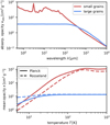 |
Fig. 1 Absorption opacities as a function of the wavelength (top) and mean opacities as a function of the temperature (bottom) for populations of small (red; |


2.3 Simulation stages
Our simulations involved three distinct stages. The first two stages assumed that the disk is symmetric along its rotational axis (thus becoming effectively 2D) and allowed us to find an equilibrium between the temperature structure of the disk and the spatial distribution of the gas and dust. The final third stage involved the main 3D run with an embedded planet.
2.3.1 2D hydrostatic relaxation
In this stage, the domain stretched from 1 to 300 au in radius and had a total opening angle of 50° in colatitude (25° per one hemisphere). We used 1024 logarithmically spaced grid cells in radius and 192 uniformly spaced grid cells in colatitude. The equilibrium disk structure was searched iteratively. Starting with a fixed temperature field, we solved the equations of hydrostatic equilibrium (see e.g. Flock et al. 2016; Chrenko & Nesvorný 2020) that let us derive the distribution of ρg. To solve the hydrostatic equations, a constraint on the radial profile of the surface density has to be provided. Unless stated otherwise, we considered a smooth power-law disk described by
 (25)
(25)
With the new estimate of ρg, we updated the distribution of small and large dust grains. We used Eq. (2) for the former, and the latter was obtained as
 (26)
(26)
where z is the cylindrical vertical height above the midplane, and Hd is the scale height of large grains. We followed Dubrulle et al. (1995) and set
 (27)
(27)
where  is the pressure scale height of gas and
 (28)
(28)
is the vertically integrated form of the Stokes number.
To close one iteration, we kept the gas and dust distributions fixed and solved Eqs. (13)–(14) over a time interval ∼ 106 s (see also Melon Fuksman & Klahr 2022), thus obtaining an updated temperature profile. We then returned to calculating ρg until the relative precision between two consecutive iterations dropped below 10−5.
The boundary conditions we used to solve the equations of hydrostatic equilibrium were symmetric. In Eqs. (13)–(14), the boundary conditions for ε were symmetric as well, whereas ER was symmetrized only at the inner radial boundary and set to ER=4 σ/c(5 K)4 elsewhere. The latter condition allows the disk to cool freely by the escape of thermal radiation (see also Chrenko et al. 2024b).
2.3.2 2D hydrodynamic relaxation
In this stage, the result of the hydrostatic relaxation was remapped to a grid with a narrower radial span, ranging from 40 to 250 au. The radial domain was sampled by 400 logarithmically spaced cells. Subsequently, the full hydrodynamic model introduced in Sect. 2.1 was evolved over several hundred orbital timescales (the exact simulation time spans are specified in Sects. 3 and B).
We used the symmetric boundary conditions for ρg, ϵ, and  . The boundary for vφ and uφ was symmetric in colatitude and a Keplerian extrapolation was used in radius. The boundary for vθ and uθ was symmetric in radius, and outflow was allowed in colatitude. The condition for vr was antisymmetric in radius and symmetric in colatitude. The same was true for ur, with the exception of the inner radial boundary, where we allowed for dust outflow. For ER, we again set ER=4 σ/c(5 K)4 in colatitude, but in the radial direction, we fixed ER to values found during the hydrostatic relaxation at the respective radial distance. We chose a similar approach to calculate the radial optical depth τirr to stellar irradiation: Its value at the inner radial edge was directly informed from the hydrostatic relaxation.
Additionally, the boundaries can be supplemented with buffer zones in which quantities can be damped following de Val-Borro et al. (2006). During the hydrodynamic relaxation, damping was applied near both radial edges, keeping ρg near its hydrostatic equilibrium state and (vr, vθ) near zero. For the large dust grains, we damped  to its hydrostatic equilibrium state near the outer radial edge and thus created a reservoir that replenished the dust population by radial drift.
2.3.3 3D run with an embedded planet
The main simulation stage was initialized from the result of the hydrodynamic relaxation by copying it 1300 times in azimuth. Additionally, the velocity fields were converted into a frame that corotated with the planet. In our simulations, the orbit of the planet was kept circular and nonmigrating.
The boundary conditions remained the same as during the hydrodynamic relaxation. In order to improve numerical stability, however, we added an additional damping zone at the disk surfaces in colatitude. In these zones, we damped all dust-related quantities, vr, and vθ to the values found by hydrodynamic relaxation. Without this damping, the numerical scheme tends to occasionally crash, likely because of the extreme dust density contrast at high altitudes above the midplane (we found minimum dust densities as low as 10−180 g cm−3). It might be argued that the damping artificially inserts additional dust in the simulation that can then settle toward the midplane and affect the solution, but we verified that this effect is negligible because the dust densities are very low, as described above.
2.4 Synthetic observations
We postprocessed the results of our hydrodynamic simulations with the Monte Carlo radiative transfer code RADMC-3D7 (Dullemond et al. 2012) to produce synthetic images for CO emission lines and the dust continuum. We studied the molecular isotopologs 12CO, 13CO, and C18O and focused on their rotational transition J=2−1 with the rest frequencies ≃230.538, 220.399, and 219.560 GHz, respectively.
For our calculations with RADMC-3D, we adopted the same computational grid as in our 3D hydrodynamic simulations. We input the density distributions of both small and large dust grains and used their full frequency-dependent opacities computed with OPTOOL (Sect. 2.2). Since our hydrodynamic model is radiative, it provides a reasonable profile of the disk temperature. Moreover, it contains the effects of compressional heating, viscous heating, and accretion luminosity. Therefore, we did not recompute the temperature with RADMC-3D. In order to derive the number density of 12CO molecules, we assumed an abundance of 10−4 relative to H2. The isotopic ratios for the remaining molecules were [12C]/[13C] = 77 and [16O]/[18O] = 560 (Wilson & Rood 1994). The population levels were calculated in local thermodynamic equilibrium using the molecular data from the LAMDA8 database (Schöier et al. 2005). We ignored the effects of microturbulence (which might affect the line profiles) and photodissociation (which might affect the molecular abundances in the upper disk layers that are exposed to highenergy radiation). An important effect that we included, albeit using a primitive scaling, was the freeze-out of CO molecules. In all locations in which the temperature was T ≤ 21 K (e.g. Schwarz et al. 2016; Pinte et al. 2018a), we reduced the molecular abundance by a scaling factor ffreeze=10−5 (e.g. Barraza-Alfaro et al. 2024).
Unless stated otherwise, our synthetic images were generated assuming disk inclination i=45° and distance ddisk=100 pc. Scattering effects were neglected for simplicity.
Summary of the parameters of our nominal hydrodynamic simulation.
3 Nominal simulation
Our nominal simulation was based on parameters that are summarized in Table 1 and included a Jupiter-mass planet (Mp= 1 MJup) orbiting at rp=120 au. At the given distance, our resolution led to grid cells that were nearly cube-shaped, which helped to minimize numerical anisotropy, especially for the radiation and dust diffusion. The Hill sphere of the planet was resolved by 30 cells in each dimension. The considered mass-doubling time of the planet, tacc=0.1 Myr, translates to the planetary luminosity Lp=2.8 × 10⁻³ L☉ or the effective surface temperature Tp,e ⋍ 4000 K (assuming the bulk density of the planet ρp = 1 g cm−3p). Placing this temperature in the context of previous works dedicated to studying the circumplanetary region at high resolution, we recall that Ayliffe & Bate (2009) found peak temperatures ∼ 4500 K and Szulágyi (2017) considered ∼ 1000−10 000 K.
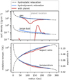 |
Fig. 2 Azimuthally averaged radial profiles in our nominal simulation with a Jupiter-mass planet. Top: vertically integrated surface density of gas and large dust. Bottom: midplane temperature (primary vertical axis) and aspect ratio (secondary vertical axis). We show the final state after the hydrostatic relaxation (dotted black curve), the hydrodynamic relaxation (solid blue curve), and the main stage with the embedded planet (solid red curve). The planet location is marked with the dashed vertical line. |
3.1 Global disk structure
Figure 2 shows 1D azimuthally averaged profiles of several characteristic quantities at the end of the simulation stages introduced in Sect. 2.3. The hydrodynamic relaxation stage covered 200 orbits, and the main run including the planet spanned 800 orbits. The planet mass and luminosity were gradually increased over the first 50 orbits of the main run9. Clearly, the proximity of curves corresponding to the hydrostatic and hydrodynamic relaxation indicates that the former is already a decent estimate of the equilibrium disk structure. The only noticeable difference arises for the surface density of large dust grains,  , because
  was set constant during the hydrostatic relaxation. This does not necessarily imply a radially uniform mass flux of dust during hydrodynamic calculations, however, because of radial variations of the Stokes number and of the pressure gradient of the nonisothermal gaseous component (for analytical arguments, see appendix A of Chrenko et al. 2024a).
Based on the profile of the aspect ratio, it is important to assess (i) whether the vertical span of the domain is larger than the typical height of the main CO emitting surfaces and (ii) how well we resolve the settled dusty layer of large grains. At the planet location, the aspect ratio is hp ≃ 0.09, implying a local pressure scale height Hp ≃ 11 au. Since the line-forming surfaces of CO are typically located at ≃ 2−4 H (Law et al. 2022), we are indeed able to capture them because the vertical boundary of our domain reaches ≃5 H. Concerning point (ii), the typical Stokes number at the planet location is Stp ≃ 0.014, which results in Hd,p ⋍ 0.19 Hp (Eq. (27)). One scale height of large grains is thus sampled by four grid cells. This resolution is rather poor, but given the global nature of our simulation and its relatively long time span, we consider it a reasonable compromise between accuracy and computational demands10.
Figure 2 also reveals that the planet carves a gas gap whose outer edge acts as an efficient trap for inward-drifting large grains. These grains pile up at r ≃ 170 au and are nearly absent from the inner disk. The global impact of the planet on the azimuthally averaged temperature profile is marginal (but see Sect. 3.2), only the gap region becomes slightly cooler on average. This is due to the excavation of the gap region, which reduces the grazing angle of the surface where most of the irradiating photons are absorbed; basically, the gap region is weakly shadowed by the inner gap edge. It is important to point out here, however, that the planetary gap is relatively shallow even though it is carved by a Jupiter-mass perturber because the planet only marginally exceeds the local thermal mass Mth=h3 M★ (Goodman & Rafikov 2001). It has Mp/Mth ⋍ 1.4, as dictated by the large local scale height hp.
The distribution of Σg and  in the r−φ plane is shown in Fig. 3. In addition to showing the structure of the gas gap and the dust ring in detail, it also enables us to study the gas and dust concentration within the Hill sphere of the planet. The local peak of the gas density is rather modest (e.g., compared to what is typically seen in locally isothermal simulations) due to the energy output of the planet, which adds to the pressure support. The large dust grains are absent from the circumplanetary region owing to the dust trap at the outer gap edge and to the midplane outflows discussed in Sect. 4.3.
3.2 Warm CO bubble surrounding the planet
Figure 4 (left panel) shows the disk temperature in a meridional plane passing through the position of the planet. The disk exhibits a layered structure that is typical for stellar irradiated disks (e.g. Chiang & Goldreich 1997; Bitsch et al. 2013; Flock et al. 2013), with a colder interior below a warmer atmosphere. The atmosphere is where the stellar photons stream freely until they are gradually absorbed, as marked by the dashed black curve. which is the surface at which the radially integrated optical depth to stellar irradiation becomes τirr=3.
The most important feature in the temperature profile is the warm bubble that surrounds the luminous planet. The extent of the isosurfaces (red curves) at which T=21 K, which is the CO freeze-out temperature we assumed (Schwarz et al. 2016; Pinte et al. 2018a), clearly shows that the thermal feedback of the planet protects CO molecules from freeze-out in a region that is slightly larger than the Hill sphere (for our nominal set of parameters). When we convert the gas density into the number density of various CO isotopologs (see Sect. 2.4), the number density within the warm bubble therefore remains higher by the factor 1/ffreeze than for the majority of the disk interior at r ≳ 70 au.
The right panel of Fig. 4 compares the vertical distribution of small and large dust grains and again shows the filtering of large grains at the planet-induced pressure bump, as well as the difference in the vertical settling between the two populations. The importance of the dust distributions for the temperature profile is such that the small grains determine the location of the τirr=3 surface, whereas the presence (or absence) of large grains is significant for the local rate of radiative cooling, as we further explore in Appendix B.
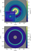 |
Fig. 3 Surface density distribution of gas (top) and large dust grains (bottom) at the end of our nominal simulation. The width of the inset in the top panel is 30 au. |
4 Observability
4.1 Synthetic images
Figure 5 provides an overview of synthetic images that we obtained by post-processing the results of our nominal simulation with RADMC-3D. Panel a shows that the warm bubble surrounding the accreting planet clearly stands out in C18O emission and appears as a low-intensity spot with a considerable solid angle. The edges of the dragonfly wings, the void in-between them, and the bubble itself directly trace the features of the temperature map shown in Fig. 4.
Panel b of Fig. 5, in which we did not account for freeze-out when we converted the simulation data into the number density of C18O, reveals that all information about the circumplanetary region is lost without freeze-out. In this case, the edges of the dragonfly wings are connected by a wall of low-intensity emission that arises from the cold disk interior. The interior layers of CO also extinct the backside of the dragonfly wing, which only remains visible as a narrow arc (see also Dullemond et al. 2020).
Panel c of Fig. 5 shows the emission of the 13CO isotopolog. 13CO is generally more abundant than C18O, and it therefore becomes optically thick already at higher elevations above the midplane. For this reason, the dragonfly wings probe a slightly warmer layer in our simulation and appear to be brighter than C18O (we used the same extent of the color scale in panels a–c to facilitate the comparison, but at the expense of saturating the 13CO image). The higher abundance of 13CO also partially obscures the bubble by the foreside surface layer at the given geometry, suggesting that C18O is more favorable for distinguishing the bubble from the extended disk emission (which is confirmed in Sect. 4.2). On its own, the bubble itself appears to be nearly identical to C18O because the optical thickness of unity is reached already at the outskirts of the bubble for all isotopologs. Therefore, the observed emission originates at gas temperatures that are only slightly above 21 K (see Fig. 4, where the bubble is warmest in its center and becomes cooler toward its edges). The bubble then appears faint and exhibits a similar emission intensity for all isotopologs. However, the bubble can become brighter when it is positioned at a channel edge as we show in the following section.
4.2 Synthetic ALMA data cubes and subtraction of the axial flow
Actual observations are filtered by the instrument response and include noise. We neglected systematic errors due to sparse u v plane sampling and assumed that these biases can be overcome with an adequate processing of ALMA high-fidelity imaging data. We also chose a beam matched to the Hill sphere size of a Jupiter-mass body at ∼ 100 au. A larger beam would improve the signal-to-noise ratio (S/N) of the disk emission, but at the expense of diluting the planetary signal. The point-spread function (PSF) was thus taken to be a circular Gaussian 70 mas in full width at half-maximum (FWHM). The radiative transfer images in native resolution were degraded with the addition of thermal noise, corresponding to the target root mean square (rms) noise amplified by a factor close to  , where N is the number of pixels in the solid angle covered by the Gaussian beam. The noise amplification factor was calibrated on a blank image, and it thus ensured the target noise level in the smoothed data cube.
For example, in the case of C18O(2−1), the ALMA sensitivity calculator (Remijan et al. 2019) yields an expected noise of 0.37 mJy beam −1 under ideal conditions in a 0.2 km s−1 bandwidth and with a 2 d integration time, which we regard as a practical maximum on sensitivity. In this application of RADMC-3D, we directly sampled the data cube at intervals of 0.04 km s−1 and then binned the spectral direction into 0.2 km s−1 channels (i.e., we averaged five native radiative transfer channels). Selected synthetic channels covering the signal from circumplanetary material are shown in the top row of Fig. 6.
The warm CO bubble is readily identified by visual inspection, for instance, at v=1.2 km s−1. It is surrounded by the extended and structured disk emission, however, which would hamper its detection in automatized searches. The unresolved signal of the bubble can be made more conspicuous by subtracting the disk emission. The same tools that are used for the kinematic planet searches can be applied to build such a background model data cube, stemming from an axially averaged disk. We used the package DISCKIN (Casassus et al., in prep.), which extracts the disk rotation curve by assuming axially symmetric line formation surfaces in the local thermodynamic equilibrium and includes meridional flows. In the case at hand, for C18O(2−1), these surfaces approximate the CO layers on either side of the frozen midplane beyond a minimum radius Rfreeze (which is a free parameter), but include the midplane layer interior to Rfreeze. The inference of the nonparametric radial profiles follows from the package CONEROT (Casassus & Pérez 2019; Casassus et al. 2021), but was derived from a leastsquares fit to the entire data cube rather than the velocity centroid images. The structure and physical conditions in the underlying axially symmetric DISCKIN model will be benchmarked against the input hydrodynamics in an upcoming article.
Based on the axially averaged channel maps, labeled Imodel in Fig. 6, we subtracted the extended disk emission and used the residuals to search for significant point sources (PSs). The systematic errors due to nonthermal residuals dominated, and we therefore applied a median filter to the residuals Iobs−Imodel (third row in Fig. 6) in order to detect a point-like signal. We used a square kernel of five times the beam width on each side and selected pixels that deviated by more than 3 σ from the median-filtered image, where the standard deviation σ was computed in each channel. The resulting PS residuals are shown in the fourth row of Fig. 6. The peak PS residual is at 9 σ at +1.6 km s−1, and the bubble is readily identified in that channel. The bubble is fainter in the other channels and reaches 6 σ at +1.2 km s−1 and +1.4 km s−1, where it can be confused with other ≲ 4 σ point-like structures from the disk.
It is interesting to note that the bubble is brighter at velocities corresponding to the edges of the channel maps. This is due to the sampling of the larger nonaxial velocity deviations closer to the accreting body, which stem from the hotter gas inside the bubble. By contrast, at disk velocities, the bubble covers a larger extent at lower brightness temperatures. The large solid angle should be favorable to its detection (see panel a of Fig. 5). However, the disk is nearly Keplerian at the co-orbital radius and the bubble is confused with disk emission. The DISCKIN kinematic model then adjusts the parameters to fit the bubble as part of the axially symmetric channel maps, which further decreases its brightness in the residuals. This rather surprising effect is due to the extension of the bubble at disk velocities, where it merges with the disk emission.
Figure 7 demonstrates this brightening of the bubble at an idealized resolution and without noise. To allow for a direct comparison with Fig. 5, we used the same channel, but rotated the hydrodynamic model so that only a part of the flow within the bubble contributed to the emission. Consequently, the bubble is divided in half and the emission probes closer to its warmer central parts that deviate more strongly from the mean disk rotation.
Another interesting aspect of our analysis of the observable kinematics is that the emergent data cubes can be reproduced almost entirely with an axially symmetric flow. The residuals in the symmetric velocity channels in Fig. 6 (bottom row) barely skim the 3 σ level even in this extremely deep and idealized observation. In other words, the residuals in a more standard observation, with a few hours of integration, would be entirely thermal. Thus, the nonaxisymmetric kinematic perturbations that are due to the gravitational perturbations induced by a body that marginally exceeds the local thermal mass are not detectable. We note, however, that the modulation of the azimuthal rotation curve due to variable hydrostatic support across the gap, as described by Teague et al. (2018), is indeed readily detected in the axially symmetric kinematics.
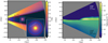 |
Fig. 4 Meridional profile of the disk temperature (left) and the volume density of small (right, bottom half) and large dust grains (right, upper half). The displayed plane coincides with the location of the planet. The temperature map also shows the isosurfaces at which T=21 K (solid red curve) and the optical depth to stellar irradiation becomes τirr=3 (dashed black curve). The width of the inset, in which we also mark the Hill sphere of the planet (dotted blue curve), is 24 au. The accreting planet heats its surroundings and maintains a bubble within which T>21 K and the freeze-out of CO molecules is prevented, unlike in the majority of the disk interior. |
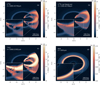 |
Fig. 5 Synthetic RADMC-3D images based on our nominal simulation. The disk inclination is 45°, and the angular position of the planet is 45° clockwise from the disk major axis. (a) Example channel map of C18O. The inset shows the CO bubble in detail. (b) As in the first panel, but ignoring freeze-out. (c) Example channel map of 13CO. (d) Dust continuum emission at 1 mm. Each image also contains the wavelength at which it was taken. The width of the inset is 1.3 arcsec. The color scale, which represents the emission intensity, is kept fixed between panels a-c. |
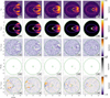 |
Fig. 6 Analysis of synthetic ALMA data cubes. Top row: filtered sky images in C18O(2−1) for selected channels. Second row: axially symmetric model data cube obtained with DISCKIN. Third row: residuals. Fourth row: point-source residuals after median filtering (see text), with the peaks from 1.0 to 1.6 km s−1 corresponding to the CO bubble and reaching 9 σ significance relative to the scatter in the residuals. Bottom row: symmetric velocity channels relative to the systemic velocity. The data cubes have been averaged into coarse sky pixels, whose solid angle approximates that of the beam, as a means to speed up the DISCKIN optimization. |
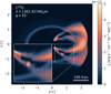 |
Fig. 7 As panel a of Fig. 5, but the underlying hydrodynamic model is rotated 10° toward the minor axis of the sky projection (φ=55° compared to 45° in Fig. 5). An animated version scanning a broader range of rotations is available online. |
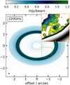 |
Fig. 8 Synthetic ALMA observation of the 220 GHz continuum in our nominal simulation with thermal noise, but without u v-plane filtering. The inset is centered on the circumplanetary environment, which is barely recognizable (at 8 σ, but confused with structures along the planetary wake). A beam ellipse is shown in the bottom left corner and also in the inset. The contour levels in the inset start at 3 σ and then rise by one σ in alternating colors. The color stretch in the figure and the grayscale in the inset are linear and cover the full range of intensities. The tick marks in the inset are placed at 0.3′′ intervals. |
4.3 Continuum emission and the depletion of circumplanetary dust
In addition to the molecular emission, the channel maps contain a ring that corresponds to the underlying dust continuum emission of large grains that accumulate at the outer edge of the planet-induced gap. To examine the dust emission in detail, we show a synthetic image at λ=1 mm in panel d of Fig. 5. In addition to the ring itself, there is an emission void interior to it and a faint skirt exterior to it. The latter is due to dust grains that we continued to reintroduce at the outer edge of the disk during the entire simulation. Importantly, the warm circumplanetary region is not detected in the thermal dust emission because there is a paucity of large dust grains in the circumplanetary region.
To further confirm the emission topology of Fig. 5d, we generated a synthetic ALMA continuum observation. We followed the same procedure as in Sect. 4.2, but used a 7.5 GHz bandwidth to reach a thermal noise of 1.7 μJy beam−1 in the continuum underlying C18O(2−1)(220 GHz), following a 2 d integration in the best conditions. Fig. 8 shows that even in this ideal observation with perfect calibration and no synthesis imaging artifacts11, the environment surrounding the protoplanet would be barely detected because only the planetary wake would be picked up as a noisy filament (resembling the noisy filament in HD 135344B; Casassus et al. 2021). Trials at the lower disk inclination of i= 30 deg showed that the protoplanet would be entirely undetected in the same setup. The fact that the circumplanetary environment of the marginally superthermal planet resulting from our gasdust hydrodynamic simulation would remain undetected even in deep ALMA observations (except barely in the ideal 2 d integration considered here) is in contrast with several previous simulation-based predictions (see Sect. 1) and is fully consistent with the paucity of CPD detections.
To understand why the large dust grains are missing, we examined the evolution of the circumplanetary dust content and found that it decays in time. Fig. 9 (left panel) shows the circumplanetary density distribution of large dust at an earlier simulation time, t=375 orbits. Apparently, the concentration of large dust grains surrounding the planet is relatively large early on: The planet is able to accumulate these grains before the gap region is fully cleared of them and their radial flux is diminished. However, Fig. 9 reveals that dust grains can leak from the central overdensity that surrounds the planet by entering the horseshoe flow as it U-turns deep within the Hill sphere. An increased dust density is evident mainly along the downstream horseshoe flow that trails the planet (in the x>120 and y<0 au quadrant). To confirm that this outflow plays a decisive role in the circumplanetary dust depletion, we performed an extended analysis of the dust mass flux in Appendix A.
The temporal evolution of the circumplanetary dust content is reflected in the dust continuum emission. The second panel of Fig. 9 shows that the warmed-up circumplanetary dust manifests itself as a hot spot at t=375 orbits. After approximately t ⋍ 450 orbits, however, the dust depletion via horseshoe flows leads to a disappearance of the hot spot, and the thermal continuum image becomes more similar to panel d of Fig. 5.
The dust flow in the close proximity of the planet can still effectively exchange material with the horseshoe flow because no full-fledged CPD is formed for the given combination of planet mass, disk conditions, and accretion heating. Additional differences between the circumplanetary environment in our nominal model and classical CPDs are highlighted in Fig. 10, where we identify a two-sided polar outflow in the meridional plane. The gas and dust both follow this outflowing pattern, as reflected by the formation of two dusty plumes that rise above the orbital plane. The polar outflow can only entrain dust grains at heights that are already relatively dust poor, however, and thus, the plumes themselves do not substantially contribute to the depletion of the circumplanetary dust content (the dust-to-gas ratio in the plumes is lower by roughly four orders of magnitude than the dust accumulation surrounding the planet).
Last but not least, it is worth noting that even in the absence of accretion heating, the Jupiter-mass planet would not be capable of forming a full-fledged CPD at rp=120 au within our disk model. The level of vertical gas compression inside the Hill sphere would instead remain only moderate and transition between a quasi-spherical envelope and a highly compressed local disk (see also Sagynbayeva et al. 2024). This is further documented in Appendix B.4.
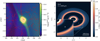 |
Fig. 9 Left: logarithm of the midplane density of large dust |

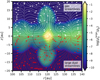 |
Fig. 10 Logarithm of the vertical dust-to-gas ratio |

5 Discussion and conclusions
We studied the influence of a luminous accreting protoplanet on the CO emission arising from a protoplanetary disk. We developed an advanced 3D radiation hydrodynamics model involving both gas and dust in a two-fluid approximation. We assumed that small (submicron-sized) dust grains passively trace the gas distribution, and we evolved large (millimeter-sized) dust grains directly, using both grain populations to derive optical depths to stellar irradiation and thermal radiation diffusion. As our nominal case, we chose a Jupiter-mass planet with an effective temperature Tp,e = 4000 K that orbited at rp=120 au. In our disk model, the ratio of the planet mass to the local thermal mass was about unity. The orbital radius fell outside the CO snowline, into a cold layer in which CO molecules freeze out and are only present in low abundances.
The accretion luminosity of the planet heats its vicinity, where it maintains a bubble of warm gas with temperatures above the freeze-out threshold (we assumed 21 K; Schwarz et al. 2016; Pinte et al. 2018a). Consequently, the abundance of gasphase CO molecules within the bubble remains higher than in the broad cold background. By inspecting synthetic CO channel maps, we found that the bubble can be readily detected by subtracting an axially symmetric kinematic disk profile and applying median filtering. The peak residual identifies the bubble as a point source located within the emission void between the foreand backside line-forming surfaces. This requires that the disk is moderately inclined (i ≈ 45°), the planet is not too close to the minor axis of the disk, and the extended disk emission does not blend with (or extincts) the bubble. The latter constraint favors rarer isotopologs such as C18O, which can become optically thin in the planetary gap region.
Since the bubble itself is optically thick, its emission is faint because it originates from the outer shells that are only marginally warmer than the freeze-out temperature. For the same reason, its emission intensity is nearly independent of the generating isotopolog.
In addition to the nominal simulation, we presented a modest suite of additional runs in Appendix B. They demonstrate that (i) the bubble shrinks when the accretion luminosity decreases, which can be counteracted by modifying the opacity law (e.g.. by assuming a higher-than-nominal constant opacity); (ii) when the planet is shifted just outside the CO snowline, the bubble can locally perturb the shape of the snowline itself; (iii) the bubble can form around subthermal-mass planets as well, but it is small and hardly detectable then (for a single value of the mass-doubling time that we tested).
Since our model tracks the evolution of mm-sized dust grains, it also provides predictions for the thermal continuum emission. In this regard, we captured the formation of a dusty ring in a pressure bump at the outer edge of the planetary gap, as well as the depletion of dust from the circumplanetary region by the downstream horseshoe flow. Therefore, the detectability of circumplanetary dust in the continuum depends on the level of depletion, exhibiting a hot spot during the first ⋍ 450 orbits, but showing no substantial signal at later times. This dust depletion might explain why circumplanetary dusty regions are observationally elusive.
We emphasize that in addition to the continuum nondetection, the marginally superthermal planet does not produce detectable velocity kinks. The resurgence of gaseous CO driven by thermal accretion feedback thus offers promising prospects for automated protoplanet detections that would otherwise seem impossible. Additionally, detections of CO bubbles would also provide crucial insights into the chemical processes that occur within circumplanetary environments, bridging the early stages of formation with the final properties of (exo)planets (e.g. Öberg et al. 2011). Our study adds to previous efforts to link the accretion luminosity of forming planets to the observable chemistry (Cleeves et al. 2015; Jiang et al. 2023) or to disk kinematics (Muley et al. 2024).
Although our work represents an important step toward an improved realism of simulated molecular and continuum emission, it includes several caveats. Regarding the molecular emission, no chemical module was involved in our calculations, and thus, the molecular abundances and the freeze-out effect depend on our choice of scaling factors when the simulated gas density is converted into the number density of the respective isotopologs. Moreover, we assumed instantaneous freeze-out and sublimation, based on the local temperature. In future work, we would like to understand whether the disk shear can distort the bubble shape or even spread it over a larger area (see Jiang et al. 2023). Finally, the accretion luminosity, which is of critical importance for the formation of the bubble, is parametric and was not obtained in a self-consistent manner.
Data availability
Movie associated to Fig. 7 is available at https://www.aanda.org
Acknowledgements
We wish to thank the anonymous referee whose constructive comments allowed us to improve the manuscript. This work was supported by the Czech Science Foundation (grant 25-16507S), the Charles University Research Centre program (No. UNCE/24/SCI/005), and the Ministry of Education, Youth and Sports of the Czech Republic through the e-INFRA CZ (ID:90254). S.C. acknowledges support from Agencia Nacional de Investigación y Desarrollo de Chile (ANID) given by FONDECYT Regular grants 1211496 and ANID project Data Observatory Foundation DO210001. The authors are grateful to Marcelo Barraza-Alfaro, Sebastiaan Krijt, and Mario Flock for useful and motivating discussions. We acknowledge the use of PYTHON libraries MATPLOTLIB (Hunter 2007), NUMPY (Harris et al. 2020), and LIC (https://gitlab.com/szs/lic).
Appendix A Dust depletion analysis
In Sect. 4.3, we suggested that the main pathway through which large dust grains leave the circumplanetary environment is via the horseshoe flow. As an additional confirmation, here we analyze the mass flux of large dust grains at various simulation times. To this end, we first constructed a planetocentric spherical grid and mapped (ρg, v) onto it using trilinear interpolation. Second, we calculated the radial mass flux of large dust defined in the new planetocentric coordinates as
 (A.1)
(A.1)
where upc,r is the radial velocity of large dust grains with respect to the planet. The negative sign in Eq. (A.1) implies that  when large dust is moving towards the planet (upc,r <0) and
  when dust is moving away from the planet (upc, r>0).
Fig. A.1 (top row) shows the time evolution of  . Despite the fact that the radial mass flux of dust is headed towards the planet in the majority of the inner Hill sphere, there is a persistent outflow channel trailing the planet location (near x=xp and y < yp) and connecting to the rear horseshoe flow (compare with the flow topology shown in the bottom row of Fig. A.1). The magnitude of this outflow does not seem to diminish over the displayed interval t=375−425 orbits, contrary to the rest of the flow across the Hill radius which decreases over time as a natural consequence of pressure bump filtering. This confirms the dominant role of the rear horseshoe flow in depleting the dust accumulation surrounding the planet. Turbulent dust diffusion, which is included in our numerical model, likely aids the process because it keeps the central dust accumulation spread-out rather than sharply centrally peaked.
Finally, we point out that we also analyzed  in the meridional plane, motivated by the presence of polar outflows in Fig. 10, but did not find an out-flowing mass flux of a magnitude comparable to that shown in Fig. A.1.
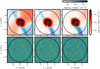 |
Fig. A.1 Top: Midplane radial mass flux of large dust grains in a planetocentric coordinate frame. The composite color gradient shows log |


Appendix B Additional simulations
The nominal simulation discussed in the main body of the paper is based on several conceptual and parametric choices that could be perceived as rather extreme. These are mainly
a relatively strong energy output of the planet (Tp,e ⋍ 4000 K) and,
the very existence of a massive Jupiter-like planet at a large orbital separation (rp=120 au).
In this Appendix, we present four additional simulations that we selected to demonstrate how the CO bubble changes when points (1.) and (2.) are modified. Additionally, we compare the nominal simulation to a case of a nonaccreting planet (Lp=0) in order to discuss its ability to form a CPD. A brief overview of the additional simulations is provided in Table B. 1 while a detailed explanation is given in the following.
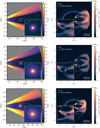 |
Fig. B.1 Meridional profiles of the disk temperature (left) and synthetic channel maps of C18O emission (right) for simulations S1 (top), S2 (middle), and S3 (bottom). Please note that the planet is shifted to 85 au in the bottom row. Therefore, the radial extent of the simulated disk, the wavelength of the synthetic image, and the centering of the inset differ from simulations S1 and S2. |
B.1 Simulations S1 and S2
Regarding point (1.), some level of degeneracy is expected between the luminosity of the planet and the opacity law, with the latter controlling the cooling rate of the planet’s vicinity. On one hand, when decreasing Lp, the size of the bubble should shrink as the local heating source for the gas weakens. On the other hand, assuming a different opacity law might help spreading the hot spot over a larger distance via radiative diffusion and thus compensate for the decrease in Lp. With this in mind, we conducted two additional simulations. Simulation labeled S1 differs from the nominal simulation in the mass doubling time of the planet, which is increased to tacc=0.5 Myr. The accretion luminosity and effective temperature decrease to Lp ⋍ 5 × 10⁻⁴ L☉ and Tp,e ⋍ 2650 K, respectively. Simulation labeled S2 has the same less efficient accretion as S1 but the opacity is set to uniform values κP=κR=1 cm2 g−1 and κ★=3 cm2 g−1 per gram of gas. We evolve only gas in simulation S2 because the influence of large grains on the opacity is not considered. Additionally, it was necessary to perform the hydrostatic and hydrodynamic relaxations for simulation S2 again because the change in the opacity leads to a slightly different equilibrium disk profile.
Summary of differences between additional simulations discussed in Appendix B and the nominal simulation.
The resulting temperature profiles and C18O channel maps for simulations S1 and S2 are shown in Fig. B.1 (top and middle rows, respectively). In simulation S1, the diameter of the bubble shrinks to 45% compared to our nominal simulation. However, the shrinkage can indeed be thwarted by a change in the opacity law, as resulting from simulation S2 in which the bubble diameter retains 73% of the nominal extent.
The behavior demonstrated by simulations S1 and S2 implies that the extent of the bubble critically depends not only on the accretion luminosity, but also on the optical thickness of the circumplanetary region to escaping thermal radiation. The optical thickness can be changed not only due to the opacity but also due to a change in the dust content (note that the opacity in simulation S1 is tied to the abundance of large dust grains, which becomes low close to the planet). Therefore, future models should strive for a detailed understanding of dust accumulation close to the planet across a wide range of grain sizes.
B.2 Simulation S3
Returning to point (2.), there are essentially two possibilities to modify our nominal assumption. First, perhaps the likelihood of forming a Jupiter-mass planet is larger closer to the star. Our nominal simulation does allow for some wiggle room as the planet can be shifted inwards and still end up outside the CO snowline. Therefore, we performed simulation S3 in which the Jupiter-mass planet was placed at rpl=85 au and the radial span of the domain was rescaled accordingly, ranging from 28 to 180 au. Second, it might be worth exploring the accretion feedback from subthermal-mass planets, which is done in Sect. B.3.
The results of simulation S3 are displayed in Fig. B.1 (bottom row). The size of the bubble is similar to the nominal simulation, which is not surprising since we only changed the planet’s orbital radius. However, due to its proximity to the CO snowline, the bubble partially merges with it. Subsequently, when looking at the synthetic image, the bubble appears to be attached to one of the wedges which fill out the space between the dragonfly wings.
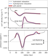 |
Fig. B.2 Top: As in the upper panel of Fig. 2, but for simulation S4 in which we introduce a putative gap in the gas disk before inserting a subthermal-mass planet. The planet is introduced and evolved inside the dusty ring occurring at the outer edge of the putative gap. Bottom: Radial profile of the pressure support parameter η= −1/2(H/r)2 ∂ log P/∂ log r (e.g. Nakagawa et al. 1986; Bitsch et al. 2018) which delimits regions of sub- and super-Keplerian rotation. |
B.3 Simulation S4
Recent theoretical works suggest that pressure bumps with dusty rings can promote fast growth of low-mass embryos until they reach masses of giant-planet cores. For instance, considering pressure bumps at ∼ 70 au distances, Lau et al. (2022) and Jiang & Ormel (2023) showed that planets growing by pebble and planetesimal accretion reach Mp ∼ 20 M⊕ on a timescale ∼ 0.1 Myr. Therefore, instead of a Jupiter-mass planet, one could argue for subthermal-mass planets to be more easier to assemble in the outermost disk regions, while also exhibiting nonzero accretion luminosities.
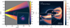 |
Fig. B.3 Meridional profiles of the disk temperature (left) and synthetic channel maps of C18O emission (right) for simulation S4 in which a subthermal-mass planet evolves in a dusty ring. |
Motivated by these findings, we designed simulation labeled S4 to study the CO bubble around a Mp=20 M⊕ planet, having the mass doubling time tacc=0.1 Myr and being positioned within a dust-loaded pressure bump. To place a putative bump in the disk before the planet is introduced, we modify Eq. (25) by carving a Gaussian gap in the surface density profile(Pinilla et al. 2012; Dullemond et al. 2018; Chrenko & Chametla 2023):
![Mathematical equation: $\Sigma_{\mathrm{g}}^{\prime}=\Sigma_{\mathrm{g}}\left[1+\left(A_{\mathrm{g}}-1\right) \exp \left(-\frac{\left(r-r_{\mathrm{g}}\right)^{2}}{2 \omega_{\mathrm{g}}^{2}}\right)\right]^{-1},$](/articles/aa/full_html/2025/08/aa54623-25/aa54623-25-eq61.png) (B.1)
(B.1)
where Ag is the amplitude of the gap, rg is the radial centre of the perturbation, and wg sets the width of the Gaussian. We note that an opposite perturbation (i.e. a peak) in the disk viscosity
![Mathematical equation: $v^{\prime}=v\left[1+\left(A_{\mathrm{g}}-1\right) \exp \left(-\frac{\left(r-r_{\mathrm{g}}\right)^{2}}{2 w_{\mathrm{g}}^{2}}\right)\right],$](/articles/aa/full_html/2025/08/aa54623-25/aa54623-25-eq62.png) (B.2)
(B.2)
has to be considered to ensure stability of the gap profile on a viscous time scale. At the outer edge of the gap, a pressure bump forms (similarly to a planet-induced gap) and becomes loaded by large dust grains (Fig. B.2).
Compared to the nominal simulation, we ran the hydrodynamic relaxation stage for 800 orbits. At the end of the relaxation, the peak increase of  in the pressure bump was by a factor of 20 with respect to initial conditions (see Fig. B.2). The main stage with the planet was shortened to 25 orbits because the given planet mass perturbs the disk only weakly. During the simulation, we removed some large dust from the immediate vicinity of the planet in order to keep the dust-to-gas ratio below 90%. This removed dust was not added to the mass of the planet, nor was it linked to the accretion luminosity (we kept it parametric).
Looking at Fig. B.3, the diameter of the CO bubble is quite small, dropping to 30% compared to the nominal case. This is because the accretion luminosity in simulation S4 is only Lp ⋍ 2 × 10⁻⁵ L☉. Still, the diameter of the bubble is not completely negligible owing to the surrounding dense dusty ring which boosts local optical depths and helps spreading the temperature perturbation further away from the planet.
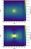 |
Fig. B.4 Logarithm of the vertical gas density distribution in the vicinity of the planet at t=375 orbits (the same orbital time as in Fig. 9). Overlaid are the streamlines of the gaseous meridional flow (red arrows), the Hill sphere (white dotted circle), and an arbitrarily chosen isosurface of log (ρg/g cm−3)=−13.5 (white dashed curve). Top: nominal simulation. Bottom: simulation Scold with a zero-luminosity planet. |
We attempted the same kinematic analysis as in Sect. 4.2. The result, however, is negative because the bubble ends up at the thermal noise level and cannot be localized as a significant point source residual. This holds even when assuming a ∼ 7 d long ALMA integration. Future work is thus needed in order to determine the minimum accretion rate of low-mass planets necessary to produce a detectable CO bubble.
B.4 Simulation Scold
To gain more insight into the structure of the circumplanetary environment, it is instructive to compare the nominal simulation with a case of a zero-luminosity planet (simulation Scold). Such a comparison is given in Fig. B.4 in terms of the vertical gas density and flow. When the planet is cold, the circumplanetary streamlines exhibit a polar inflow and equatorial outflow (e.g. Ayliffe & Bate 2009; Szulágyi et al. 2016). Nevertheless, the level of vertical gas compression and deviation from a quasispherical envelope structure is only moderate. This is related to the fact that the ratio of the planet mass to the local thermal mass (Mth=h3 M★) is close to unity, Mp/Mth ⋍ 1.4. For planets at the verge of the thermal mass, Sagynbayeva et al. (2024) recently showed that the level of circumplanetary ‘diskiness’ indeed remains only moderate (their figure 6 for h=0.1 and Mp=1 MJup can serve as a useful comparison). Their assertion that full-fledged CPDs are unlikely to form around Jupiter-mass protoplanets at large orbital separations (due to the increase of the disk’s aspect ratio) matches our findings.
When the nominal accretion luminosity is considered, the local heat release provides additional pressure support counteracting the vertical compression (see also Muley et al. 2024) and the planet is left with a quasi-spherical envelope of lowered gas density. Moreover, the polar flow topology becomes reversed compared to the zero-luminosity planet, as already mentioned in Sect. 4.3.
References
- Andrews, S. M., 2020, ARA&A, 58, 483 [Google Scholar]
- Ayliffe, B. A., & Bate, M. R., 2009, MNRAS, 397, 657 [Google Scholar]
- Bae, J., Teague, R., Andrews, S. M., et al. 2022, ApJ, 934, L20 [NASA ADS] [CrossRef] [Google Scholar]
- Bae, J., Isella, A., Zhu, Z., et al. 2023, in Astronomical Society of the Pacific Conference Series, 534, Protostars and Planets VII, eds. S. Inutsuka, Y. Aikawa, T. Muto, K. Tomida, & M. Tamura, 423 [Google Scholar]
- Barraza-Alfaro, M., Flock, M., & Henning, T., 2024, A&A, 683, A16 [NASA ADS] [CrossRef] [EDP Sciences] [Google Scholar]
- Benisty, M., Bae, J., Facchini, S., et al. 2021, ApJ, 916, L2 [NASA ADS] [CrossRef] [Google Scholar]
- Benisty, M., Dominik, C., Follette, K., et al. 2023, in Astronomical Society of the Pacific Conference Series, 534, Protostars and Planets VII, eds. S. Inutsuka, Y. Aikawa, T. Muto, K. Tomida, & M. Tamura, 605 [Google Scholar]
- Benítez-Llambay, P., & Masset, F. S., 2016, ApJS, 223, 11 [Google Scholar]
- Benítez-Llambay, P., Masset, F., Koenigsberger, G., & Szulágyi, J., 2015, Nature, 520, 63 [Google Scholar]
- Benítez-Llambay, P., Krapp, L., & Pessah, M. E., 2019, ApJS, 241, 25 [Google Scholar]
- Birnstiel, T., Dullemond, C. P., Zhu, Z., et al. 2018, ApJ, 869, L45 [CrossRef] [Google Scholar]
- Bitsch, B., Crida, A., Morbidelli, A., Kley, W., & Dobbs-Dixon, I., 2013, A&A, 549, A124 [NASA ADS] [CrossRef] [EDP Sciences] [Google Scholar]
- Bitsch, B., Morbidelli, A., Johansen, A., et al. 2018, A&A, 612, A30 [NASA ADS] [CrossRef] [EDP Sciences] [Google Scholar]
- Casassus, S., & Cárcamo, M., 2022, MNRAS, 513, 5790 [NASA ADS] [CrossRef] [Google Scholar]
- Casassus, S., & Pérez, S., 2019, ApJ, 883, L41 [Google Scholar]
- Casassus, S., Christiaens, V., Cárcamo, M., et al. 2021, MNRAS, 507, 3789 [CrossRef] [Google Scholar]
- Chen, K., & Dong, R., 2024, ApJ, 976, 49 [Google Scholar]
- Chiang, E. I., & Goldreich, P., 1997, ApJ, 490, 368 [Google Scholar]
- Chrenko, O., & Chametla, R. O., 2023, MNRAS, 524, 2705 [NASA ADS] [CrossRef] [Google Scholar]
- Chrenko, O., & Lambrechts, M., 2019, A&A, 626, A109 [NASA ADS] [CrossRef] [EDP Sciences] [Google Scholar]
- Chrenko, O., & Nesvorný, D., 2020, A&A, 642, A219 [NASA ADS] [CrossRef] [EDP Sciences] [Google Scholar]
- Chrenko, O., Chametla, R. O., Masset, F. S., Baruteau, C., & Brož, M. 2024a, A&A, 690, A41 [NASA ADS] [CrossRef] [EDP Sciences] [Google Scholar]
- Chrenko, O., Flock, M., Ueda, T., et al. 2024b, AJ, 167, 124 [Google Scholar]
- Christiaens, V., Samland, M., Henning, T., et al. 2024, A&A, 685, L1 [NASA ADS] [CrossRef] [EDP Sciences] [Google Scholar]
- Cleeves, L. I., Bergin, E. A., & Harries, T. J., 2015, ApJ, 807, 2 [NASA ADS] [CrossRef] [Google Scholar]
- Commerçon, B., Teyssier, R., Audit, E., Hennebelle, P., & Chabrier, G., 2011, A&A, 529, A35 [NASA ADS] [CrossRef] [EDP Sciences] [Google Scholar]
- Currie, T., Lawson, K., Schneider, G., et al. 2022, Nat. Astron., 6, 751 [NASA ADS] [CrossRef] [Google Scholar]
- Cuzzi, J. N., Dobrovolskis, A. R., & Champney, J. M., 1993, Icarus, 106, 102 [NASA ADS] [CrossRef] [Google Scholar]
- de Val-Borro, M., Edgar, R. G., Artymowicz, P., et al. 2006, MNRAS, 370, 529 [Google Scholar]
- Dipierro, G., Laibe, G., Price, D. J., & Lodato, G., 2016, MNRAS, 459, L1 [NASA ADS] [CrossRef] [Google Scholar]
- Dominik, C., Min, M., & Tazaki, R., 2021, Astrophysics Source Code Library [record ascl:2104.010] [Google Scholar]
- Dubrulle, B., Morfill, G., & Sterzik, M., 1995, Icarus, 114, 237 [Google Scholar]
- Dullemond, C. P., Juhasz, A., Pohl, A., et al. 2012, RADMC-3D: A multi-purpose radiative transfer tool [Google Scholar]
- Dullemond, C. P., Birnstiel, T., Huang, J., et al. 2018, ApJ, 869, L46 [NASA ADS] [CrossRef] [Google Scholar]
- Dullemond, C. P., Isella, A., Andrews, S. M., Skobleva, I., & Dzyurkevich, N., 2020, A&A, 633, A137 [EDP Sciences] [Google Scholar]
- Fedele, D., Bollati, F., & Lodato, G., 2023, A&A, 672, A125 [NASA ADS] [CrossRef] [EDP Sciences] [Google Scholar]
- Flock, M., Fromang, S., González, M., & Commerçon, B., 2013, A&A, 560, A43 [NASA ADS] [CrossRef] [EDP Sciences] [Google Scholar]
- Flock, M., Fromang, S., Turner, N. J., & Benisty, M., 2016, ApJ, 827, 144 [CrossRef] [Google Scholar]
- Goodman, J., & Rafikov, R. R., 2001, ApJ, 552, 793 [NASA ADS] [CrossRef] [Google Scholar]
- Haffert, S. Y., Bohn, A. J., de Boer, J., et al. 2019, Nat. Astron., 3, 749 [Google Scholar]
- Hammond, I., Christiaens, V., Price, D. J., et al. 2023, MNRAS, 522, L51 [NASA ADS] [CrossRef] [Google Scholar]
- Harris, C. R., Millman, K. J., van der Walt, S. J., et al. 2020, Nature, 585, 357 [NASA ADS] [CrossRef] [Google Scholar]
- Hunter, J. D., 2007, Comput. Sci. Eng., 9, 90 [NASA ADS] [CrossRef] [Google Scholar]
- Isella, A., Benisty, M., Teague, R., et al. 2019, ApJ, 879, L25 [Google Scholar]
- Jiang, H., & Ormel, C. W., 2023, MNRAS, 518, 3877 [Google Scholar]
- Jiang, H., Wang, Y., Ormel, C. W., Krijt, S., & Dong, R., 2023, A&A, 678, A33 [NASA ADS] [CrossRef] [EDP Sciences] [Google Scholar]
- Keppler, M., Benisty, M., Müller, A., et al. 2018, A&A, 617, A44 [NASA ADS] [CrossRef] [EDP Sciences] [Google Scholar]
- Klahr, H., & Kley, W., 2006, A&A, 445, 747 [NASA ADS] [CrossRef] [EDP Sciences] [Google Scholar]
- Kley, W., 1989, A&A, 208, 98 [NASA ADS] [Google Scholar]
- Kolb, S. M., Stute, M., Kley, W., & Mignone, A., 2013, A&A, 559, A80 [NASA ADS] [CrossRef] [EDP Sciences] [Google Scholar]
- Krapp, L., Kratter, K. M., Youdin, A. N., et al. 2024, ApJ, 973, 153 [NASA ADS] [CrossRef] [Google Scholar]
- Lau, T. C. H., Drążkowska, J., Stammler, S. M., Birnstiel, T., & Dullemond, C. P., 2022, A&A, 668, A170 [NASA ADS] [CrossRef] [EDP Sciences] [Google Scholar]
- Law, C. J., Crystian, S., Teague, R., et al. 2022, ApJ, 932, 114 [NASA ADS] [CrossRef] [Google Scholar]
- Levermore, C. D., & Pomraning, G. C., 1981, ApJ, 248, 321 [NASA ADS] [CrossRef] [Google Scholar]
- Lodato, G., Dipierro, G., Ragusa, E., et al. 2019, MNRAS, 486, 453 [Google Scholar]
- Melon Fuksman, J. D., & Klahr, H., 2022, ApJ, 936, 16 [NASA ADS] [CrossRef] [Google Scholar]
- Mihalas, D., & Weibel Mihalas, B., 1984, Foundations of Radiation Hydrodynamics (New York: Oxford University Press) [Google Scholar]
- Montesinos, M., Cuadra, J., Perez, S., Baruteau, C., & Casassus, S., 2015, ApJ, 806, 253 [NASA ADS] [CrossRef] [Google Scholar]
- Morfill, G. E., & Voelk, H. J., 1984, ApJ, 287, 371 [Google Scholar]
- Muley, D., Melon Fuksman, J. D., & Klahr, H., 2024, A&A, 687, A213 [NASA ADS] [CrossRef] [EDP Sciences] [Google Scholar]
- Nakagawa, Y., Sekiya, M., & Hayashi, C., 1986, Icarus, 67, 375 [Google Scholar]
- Öberg, K. I., Murray-Clay, R., & Bergin, E. A., 2011, ApJ, 743, L16 [Google Scholar]
- Paardekooper, S.-J., & Mellema, G., 2006, A&A, 459, L17 [CrossRef] [EDP Sciences] [Google Scholar]
- Perez, S., Dunhill, A., Casassus, S., et al. 2015, ApJ, 811, L5 [NASA ADS] [CrossRef] [Google Scholar]
- Pérez, L. M., Benisty, M., Andrews, S. M., et al. 2018, ApJ, 869, L50 [CrossRef] [Google Scholar]
- Pérez, S., Casassus, S., Hales, A., et al. 2020, ApJ, 889, L24 [Google Scholar]
- Petrovic, H. J., Booth, R. A., & Clarke, C. J., 2024, MNRAS, 534, 2412 [Google Scholar]
- Pinilla, P., & Youdin, A., 2017, in Astrophysics and Space Science Library, 445, Formation, Evolution, and Dynamics of Young Solar Systems, eds. M. Pessah & O. Gressel, 91 [Google Scholar]
- Pinilla, P., Birnstiel, T., Ricci, L., et al. 2012, A&A, 538, A114 [NASA ADS] [CrossRef] [EDP Sciences] [Google Scholar]
- Pinte, C., Ménard, F., Duchêne, G., et al. 2018a, A&A, 609, A47 [NASA ADS] [CrossRef] [EDP Sciences] [Google Scholar]
- Pinte, C., Price, D. J., Ménard, F., et al. 2018b, ApJ, 860, L13 [Google Scholar]
- Pinte, C., van der Plas, G., Ménard, F., et al. 2019, Nat. Astron., 3, 1109 [NASA ADS] [CrossRef] [Google Scholar]
- Pinte, C., Hammond, I., Price, D. J., et al. 2023, MNRAS, 526, L41 [NASA ADS] [CrossRef] [Google Scholar]
- Qi, C., & Wilner, D. J., 2024, ApJ, 977, 60 [Google Scholar]
- Qi, C., Öberg, K. I., Wilner, D. J., et al. 2013, Science, 341, 630 [Google Scholar]
- Remijan, A., Biggs, A., Cortes, P. A., et al. 2019, ALMA Technical Handbook, ALMA Doc. 7.3, ver. 1.1 [Google Scholar]
- Sagynbayeva, S., Li, R., Kuznetsova, A., et al. 2024, arXiv e-prints [arXiv:2410.14896] [Google Scholar]
- Schöier, F. L., van der Tak, F. F. S., van Dishoeck, E. F., & Black, J. H., 2005, A&A, 432, 369 [Google Scholar]
- Schwarz, K. R., Bergin, E. A., Cleeves, L. I., et al. 2016, ApJ, 823, 91 [CrossRef] [Google Scholar]
- Shakura, N. I., & Sunyaev, R. A., 1973, A&A, 500, 33 [NASA ADS] [Google Scholar]
- Stone, J. M., & Norman, M. L., 1992, ApJS, 80, 753 [Google Scholar]
- Szulágyi, J., 2017, ApJ, 842, 103 [Google Scholar]
- Szulágyi, J., Masset, F., Lega, E., et al. 2016, MNRAS, 460, 2853 [Google Scholar]
- Szulágyi, J., Plas, G. v. d., Meyer, M. R., et al. 2018, MNRAS, 473, 3573 [CrossRef] [Google Scholar]
- Teague, R., Bae, J., Bergin, E. A., Birnstiel, T., & Foreman-Mackey, D., 2018, ApJ, 860, L12 [NASA ADS] [CrossRef] [Google Scholar]
- Ueda, T., Tazaki, R., Okuzumi, S., Flock, M., & Sudarshan, P., 2024, Nat. Astron., 8, 1148 [Google Scholar]
- Wagner, K., Follete, K. B., Close, L. M., et al. 2018, ApJ, 863, L8 [Google Scholar]
- Wagner, K., Stone, J., Skemer, A., et al. 2023, Nat. Astron., 7, 1208 [CrossRef] [Google Scholar]
- Weber, P., Pérez, S., Benítez-Llambay, P., et al. 2019, ApJ, 884, 178 [NASA ADS] [CrossRef] [Google Scholar]
- Wilson, T. L., & Rood, R., 1994, ARA&A, 32, 191 [Google Scholar]
- Wolf, S., & D’Angelo, G., 2005, ApJ, 619, 1114 [NASA ADS] [CrossRef] [Google Scholar]
- Zhang, S., Zhu, Z., Huang, J., et al. 2018, ApJ, 869, L47 [Google Scholar]
- Zhang, S., Zhu, Z., Ueda, T., et al. 2023, ApJ, 953, 96 [NASA ADS] [CrossRef] [Google Scholar]
- Zhou, Y., Bowler, B. P., Wagner, K. R., et al. 2021, AJ, 161, 244 [NASA ADS] [CrossRef] [Google Scholar]
- Zhou, Y., Bowler, B. P., Sanghi, A., et al. 2025, ApJ, 980, L39 [Google Scholar]
- Zhu, Z., Nelson, R. P., Dong, R., Espaillat, C., & Hartmann, L., 2012, ApJ, 755, 6 [Google Scholar]
- Zhu, Z., Andrews, S. M., & Isella, A., 2018, MNRAS, 479, 1850 [Google Scholar]
- Ziampras, A., Sudarshan, P., Dullemond, C. P., et al. 2025, MNRAS, 536, 3322 [NASA ADS] [CrossRef] [Google Scholar]
In practice, the typical innermost working radii at which ALMA can resolve substructures are ∼ 30 au.
The location of the CO snowline can vary from one disk to the next; as an example. we quote ∼ 30 au for TW Hya (Qi et al. 2013) and ∼ 80 au for HD 163296 (Qi & Wilner 2024).
Our choice of X0 represents a moderate value and is motivated by the fact that (i) a substantially lower X0 would lead to absorption of stellar irradiation already at very high elevations above midplane, resulting in a vertically extended cold disk interior, and hence, in an extremely extended zone of frozen-out CO; (ii) a substantially higher X0 would lead to extremely low optical depths in regions that are devoid of large grains, such as within planet-induced gaps. We wished to avoid both (i) and (ii).
The Schmidt number is the ratio of the turbulent viscosity v to the dust diffusivity (Cuzzi et al. 1993).
Gas opacities were neglected in our model.
The simulated time interval with a full-grown planet (750 orbits) translates to ⋍ 1 Myr. Full convergence of the gap profile was not reached during this time, but the relative change in Σg(r) is only 5% per 100 orbits at the end of the simulation.
Our nominal simulation required six days on 24 NVIDIA A100 GPUs.
We stress that the required signal-to-noise ratio ∼ 700 have only been achieved in compact array configurations and after self-calibration. Resolved long-baseline observations with ALMA are limited by the imperfect visibility calibration (e.g., due to the phase noise) and seldom reach beyond S/N ∼ 100. However, Domínguez-Jamett et al. (in prep.) have recently reached S/N ∼ 350 observing PDS 70 with a 25 h integration in Band 7 and a similar beam as assumed here.
All Tables
Summary of differences between additional simulations discussed in Appendix B and the nominal simulation.
All Figures
|
Fig. 1 Absorption opacities as a function of the wavelength (top) and mean opacities as a function of the temperature (bottom) for populations of small (red; |
| In the text | |
|
Fig. 2 Azimuthally averaged radial profiles in our nominal simulation with a Jupiter-mass planet. Top: vertically integrated surface density of gas and large dust. Bottom: midplane temperature (primary vertical axis) and aspect ratio (secondary vertical axis). We show the final state after the hydrostatic relaxation (dotted black curve), the hydrodynamic relaxation (solid blue curve), and the main stage with the embedded planet (solid red curve). The planet location is marked with the dashed vertical line. |
| In the text | |
|
Fig. 3 Surface density distribution of gas (top) and large dust grains (bottom) at the end of our nominal simulation. The width of the inset in the top panel is 30 au. |
| In the text | |
|
Fig. 4 Meridional profile of the disk temperature (left) and the volume density of small (right, bottom half) and large dust grains (right, upper half). The displayed plane coincides with the location of the planet. The temperature map also shows the isosurfaces at which T=21 K (solid red curve) and the optical depth to stellar irradiation becomes τirr=3 (dashed black curve). The width of the inset, in which we also mark the Hill sphere of the planet (dotted blue curve), is 24 au. The accreting planet heats its surroundings and maintains a bubble within which T>21 K and the freeze-out of CO molecules is prevented, unlike in the majority of the disk interior. |
| In the text | |
|
Fig. 5 Synthetic RADMC-3D images based on our nominal simulation. The disk inclination is 45°, and the angular position of the planet is 45° clockwise from the disk major axis. (a) Example channel map of C18O. The inset shows the CO bubble in detail. (b) As in the first panel, but ignoring freeze-out. (c) Example channel map of 13CO. (d) Dust continuum emission at 1 mm. Each image also contains the wavelength at which it was taken. The width of the inset is 1.3 arcsec. The color scale, which represents the emission intensity, is kept fixed between panels a-c. |
| In the text | |
|
Fig. 6 Analysis of synthetic ALMA data cubes. Top row: filtered sky images in C18O(2−1) for selected channels. Second row: axially symmetric model data cube obtained with DISCKIN. Third row: residuals. Fourth row: point-source residuals after median filtering (see text), with the peaks from 1.0 to 1.6 km s−1 corresponding to the CO bubble and reaching 9 σ significance relative to the scatter in the residuals. Bottom row: symmetric velocity channels relative to the systemic velocity. The data cubes have been averaged into coarse sky pixels, whose solid angle approximates that of the beam, as a means to speed up the DISCKIN optimization. |
| In the text | |
|
Fig. 7 As panel a of Fig. 5, but the underlying hydrodynamic model is rotated 10° toward the minor axis of the sky projection (φ=55° compared to 45° in Fig. 5). An animated version scanning a broader range of rotations is available online. |
| In the text | |
|
Fig. 8 Synthetic ALMA observation of the 220 GHz continuum in our nominal simulation with thermal noise, but without u v-plane filtering. The inset is centered on the circumplanetary environment, which is barely recognizable (at 8 σ, but confused with structures along the planetary wake). A beam ellipse is shown in the bottom left corner and also in the inset. The contour levels in the inset start at 3 σ and then rise by one σ in alternating colors. The color stretch in the figure and the grayscale in the inset are linear and cover the full range of intensities. The tick marks in the inset are placed at 0.3′′ intervals. |
| In the text | |
|
Fig. 9 Left: logarithm of the midplane density of large dust |
| In the text | |
|
Fig. 10 Logarithm of the vertical dust-to-gas ratio |
| In the text | |
|
Fig. A.1 Top: Midplane radial mass flux of large dust grains in a planetocentric coordinate frame. The composite color gradient shows log |
| In the text | |
|
Fig. B.1 Meridional profiles of the disk temperature (left) and synthetic channel maps of C18O emission (right) for simulations S1 (top), S2 (middle), and S3 (bottom). Please note that the planet is shifted to 85 au in the bottom row. Therefore, the radial extent of the simulated disk, the wavelength of the synthetic image, and the centering of the inset differ from simulations S1 and S2. |
| In the text | |
|
Fig. B.2 Top: As in the upper panel of Fig. 2, but for simulation S4 in which we introduce a putative gap in the gas disk before inserting a subthermal-mass planet. The planet is introduced and evolved inside the dusty ring occurring at the outer edge of the putative gap. Bottom: Radial profile of the pressure support parameter η= −1/2(H/r)2 ∂ log P/∂ log r (e.g. Nakagawa et al. 1986; Bitsch et al. 2018) which delimits regions of sub- and super-Keplerian rotation. |
| In the text | |
|
Fig. B.3 Meridional profiles of the disk temperature (left) and synthetic channel maps of C18O emission (right) for simulation S4 in which a subthermal-mass planet evolves in a dusty ring. |
| In the text | |
|
Fig. B.4 Logarithm of the vertical gas density distribution in the vicinity of the planet at t=375 orbits (the same orbital time as in Fig. 9). Overlaid are the streamlines of the gaseous meridional flow (red arrows), the Hill sphere (white dotted circle), and an arbitrarily chosen isosurface of log (ρg/g cm−3)=−13.5 (white dashed curve). Top: nominal simulation. Bottom: simulation Scold with a zero-luminosity planet. |
| In the text | |
Current usage metrics show cumulative count of Article Views (full-text article views including HTML views, PDF and ePub downloads, according to the available data) and Abstracts Views on Vision4Press platform.
Data correspond to usage on the plateform after 2015. The current usage metrics is available 48-96 hours after online publication and is updated daily on week days.
Initial download of the metrics may take a while.