| Issue |
A&A
Volume 700, August 2025
|
|
|---|---|---|
| Article Number | A204 | |
| Number of page(s) | 16 | |
| Section | The Sun and the Heliosphere | |
| DOI | https://doi.org/10.1051/0004-6361/202555520 | |
| Published online | 21 August 2025 | |
Spectropolarimetric synthesis of forbidden lines in magnetohydrodynamic models of coronal bright points
1
Instituto de Astrofísica de Canarias, E-38205 La Laguna, Tenerife, Spain
2
Departamento de Astrofísica, Universidad de La Laguna, E-38206 La Laguna, Tenerife, Spain
3
Rosseland Centre for Solar Physics, University of Oslo, PO Box 1029 Blindern 0315 Oslo, Norway
4
Institute of Theoretical Astrophysics, University of Oslo, PO Box 1029 Blindern 0315 Oslo, Norway
⋆ Corresponding author: This email address is being protected from spambots. You need JavaScript enabled to view it.
Received:
14
May
2025
Accepted:
30
June
2025
Abstract
Context. The inference of the magnetic field vector from spectropolarimetric observations is crucial for understanding the physical processes governing the solar corona.
Aims. We investigated what information on the magnetic fields of coronal bright points (CBPs) can be gained from the intensity and polarization of the Fe XIII 10747 Å, Fe XIV 5303 Å, Si X 14301 Å, and Si IX 39343 Å forbidden lines.
Methods. We applied the P-CORONA synthesis code to a CBP model in the very low corona, obtained with the Bifrost code, and to a larger global model to study the impact of the outer coronal material along the line of sight (LoS).
Results. The enhanced density within the CBP produces an intensity brightening, but suppresses the linear polarization. The circular polarization from such regions often approaches 0.1% of the intensity. The relative contribution from the coronal material along the LoS depends strongly on its temperature, and is weaker for lines with a peak response at higher temperatures (Fe XIII 10747 Å at 1.7 MK and Fe XIV 5303 Å at 2 MK). The weak field approximation (WFA) provides information on the longitudinal magnetic fields in the strongest-emitting spatial intervals along the LoS, and we find it to be more reliable in the regions of the CBP where the field does not change sign. This tends to coincide with the regions where there is a strong correlation between the circular polarization and the wavelength derivative of the intensity. Considering roughly 30 minutes of time evolution, the CBP signals are somewhat attenuated, but are still clearly identifiable, and the area where the WFA can be suitably applied remains substantial.
Conclusions. The circular polarization of the Fe XIV 5303 Å and especially Fe XIII 10747 Å lines are valuable diagnostics for the magnetic fields in the higher-temperature regions of the CBP, which could be exploited with future coronagraphs with similar capabilities to Cryo-NIRSP/DKIST, but designed to observe below 1.05 R⊙.
Key words: magnetohydrodynamics (MHD) / polarization / radiative transfer / Sun: corona
© The Authors 2025
 Open Access article, published by EDP Sciences, under the terms of the Creative Commons Attribution License (https://creativecommons.org/licenses/by/4.0), which permits unrestricted use, distribution, and reproduction in any medium, provided the original work is properly cited.
This article is published in open access under the Subscribe to Open model. This email address is being protected from spambots. You need JavaScript enabled to view it. to support open access publication.
1. Introduction
Despite the importance of magnetism in the physics of the solar corona (e.g., Priest 2014; Raouafi et al. 2016; Green et al. 2018; Judge & Ionson 2024), measurements of its magnetic fields remain very scarce. Although observations of the radiation intensity can provide valuable information, often from extreme ultraviolet (EUV) lines and relying on extrapolations (e.g., Warren et al. 2018; Jarolim et al. 2023; Madjarska et al. 2024), quantitative data are much more readily available through the polarization of spectral lines (e.g., Trujillo Bueno & del Pino Alemán 2022). Remarkably, the spectral lines that arise from transitions that are not allowed by the electric-dipole selection rules (i.e., forbidden lines) are of particular interest for probing the corona. The most prominent of these lines are those produced by magnetic-dipole-type (M1) transitions between fine-structure levels of the ground term of the corresponding chemical species (Judge 1998). Thus, these lines have relatively long wavelengths, typically falling in the visible or infrared range of the spectrum.
The polarization patterns of such lines are sensitive to the magnetic field through two main physical mechanisms, the Hanle and Zeeman effects. For forbidden lines emitted in the rarefied corona, both collisional and radiative processes can contribute significantly to populating the upper level of the considered transition (Sahal-Brechot 1974; Judge 1998; Casini & Judge 1999). Collisions excite the atoms into high-energy states, from which they cascade down to the transition’s upper level. The absorption of the radiation from the solar photosphere also contributes to populate the upper level and, because this radiation field is anisotropic, population imbalances and quantum coherence arise between the magnetic sublevels (i.e., atomic polarization is produced). In particular, if the radiation induces population imbalances between sublevels with different quantum number |M| (i.e., atomic alignment), the emitted radiation is linearly polarized, in a process known as scattering polarization. Furthermore, the magnetic field tends to modify the atomic polarization by reducing the quantum interference between magnetic sublevels through the Hanle effect. Thus, the magnetic field leaves its signatures on the scattering polarization, usually by depolarizing it and rotating the plane of linear polarization (for an in-depth discussion on scattering polarization and the Hanle effect, see Trujillo Bueno 2001). The Hanle effect operates when the Larmor frequency (which is proportional to the splitting between magnetic sublevels) is comparable to the inverse lifetime of the level. For the considered forbidden lines, this occurs for fields on the order of 10−6 G or weaker. In the solar corona, where magnetic fields on the order of gauss are commonplace, such lines are in the Hanle saturation regime, and thus their scattering polarization encodes information only on the orientation of the magnetic field, but not its strength. Magnetic fields can also produce polarization signals through the Zeeman effect, by causing an energy splitting between the magnetic sublevels of the atomic levels involved in the transition. This occurs even in the absence of atomic level polarization, so both collisional processes and radiative absorption contribute to the Zeeman polarization patterns. The amplitude of the signals produced by the Zeeman effect scale with the ratio of the magnetic splitting to the width of the line, ℛ. The ratio increases linearly with the line’s wavelength and decreases with the square root of the temperature. For the typical temperatures and magnetic fields of the corona, this quantity is generally quite small, even for infrared lines with long wavelengths (taking values of ∼10−3 − 10−4). This means that linear polarization Zeeman signals (which scale with ℛ2) should be vanishingly small, but non-negligible circular polarization signals (which scale linearly with ℛ) could be expected. The detection of these latter signals was recently reported in Schad et al. (2024).
For the present work we studied the potential of the polarization of forbidden spectral lines for diagnostics of magnetic fields in fundamental structures of the lower solar corona, namely coronal bright points (CBP). The four specific forbidden lines that we studied are the green Fe XIV line at 5303 Å (hereafter Fe5303), the Fe XIII line at 10747 Å (Fe10747), the Si X line at 14301 Å (Si14301), and the Si IX line at 39343 Å (Si39343). The interest in these lines is highlighted by the multitude of observations that have been carried out in the past, especially in linear polarization (e.g., Eddy & McKim Malville 1967; Mickey 1973; Arnaud 1982; Tomczyk et al. 2007; Dima et al. 2019). In addition, in a select few investigations, measurements of the coronal magnetic field were obtained from observations in circular polarization (see Lin et al. 2004; Schad et al. 2024). Recent instruments for coronal spectropolarimetry have been designed specifically for the wavelengths corresponding to some or all of these lines, including SOLARC (Kuhn et al. 2003), UCoMP (Tomczyk et al. 2021; see also Tomczyk et al. 2008), VELC/Aditya-L1 (Singh et al. 2019), or Cryo-NIRSP/DKIST (Rimmele et al. 2020; Fehlmann et al. 2023).
In recent years, a number of theoretical investigations have been carried out on these lines, based on spectral synthesis using suitable atmospheric models. These have been enabled by the development of numerical codes that can account for three-dimensional (3D) atmospheric models and for the relevant physics (including collisional processes, scattering polarization, and the Hanle and Zeeman effects), while the medium can be treated as optically thin. For instance, the FORWARD toolset (Gibson et al. 2016) has been used to investigate a variety of permitted coronal lines (e.g., Khan et al. 2024), as well as forbidden lines, including Fe10747 (e.g., Karna et al. 2019). Li et al. (2017) used the density matrix formalism for multi-level atoms under the assumption of a flat-spectrum incident radiation field (Casini & Judge 1999, 2000; Landi Degl’Innocenti & Landolfi 2004). In the same paper, the intensity and polarization signals of the Fe10747 line were synthesized considering potential-field source-surface coronal magnetic field models. The PyCELP code (see Schad & Dima 2020, 2021), based on the same formalism, was recently applied to models obtained with the radiative magnetohydrodynamic (r-MHD) MURaM code, representative of active regions (Rempel 2017). These investigations considered six lines of interest for Cryo-NIRSP/DKIST, including the four lines studied in this work in addition to the Fe XI line at 7892 Å and the Fe XIII line at 10798 Å. The recently developed and publicly available P-CORONA code can suitably treat both forbidden and permitted spectral lines (Supriya et al. 2021, 2025). Moreover, unlike other previously mentioned codes, P-CORONA does not assume the weak field limit when accounting for the impact of the Zeeman effect. A detailed description of this code can be found in Supriya et al. (2025). That article also presents brief illustrative applications of the code to the same six lines investigated in Schad & Dima (2020, 2021), but considering atmospheric models representative of the full extended corona as well as various models obtained with the MURaM code representing different low-corona conditions.
For the present work, we used P-CORONA to examine in detail the spectropolarimetric signals of the Fe5303, Fe10747, Si14301, and Si39343 lines for the specific case of CBPs. These low-corona structures are ubiquitous in the Sun, regardless of the level of activity (Madjarska 2019), and are possibly important contributors to coronal heating (Priest et al. 1994). CBPs, composed of small loops that confine plasma heated to several million degrees, can be considered small-scale analogs of active regions (Gao et al. 2022). To investigate the polarization signals of forbidden lines produced in a CBP, we computed them numerically with P-CORONA, considering the models resulting from radiative magnetohydrodynamic (r-MHD) simulations with the Bifrost code (Gudiksen et al. 2011) carried out by Nóbrega-Siverio et al. (2023). Present-day coronagraphs such as Cryo-NIRSP/DKIST are not designed for observations less than 0.05 R⊙ from the base of the corona, where most CBPs are expected to be found, since their projected size ranges from about 5 to 40 Mm and their heights range between 5 and 10 Mm (Madjarska 2019). The main goal of this investigation is to evaluate the suitability of techniques based on the polarization of forbidden lines for studying CBP magnetic fields, thereby providing insights for future instrumental developments and observational studies.
In Sect. 2 we present the methodology that we employed, the atmospheric models that we considered, and the main assumptions that we made. In Sect. 3 we show the synthetic wavelength-integrated intensity and polarization images corresponding to emission from a CBP. In Sect. 4 we analyze how the same images are impacted by coronal material lying along the line of sight (LoS) direction. In Sect. 5 we investigate the suitability of inferring the magnetic fields in the CBP from the circular polarization signals of the emitted radiation. In Sect. 6 we consider the intensity and polarization signals produced when accounting for the time evolution of CBP. The overall conclusions are presented in Sect. 7.
2. Formulation
The four forbidden lines that we analyzed in this work arise from M1 transitions between different J levels of the ground term of their corresponding chemical species. The atomic parameters for the lines of interest are shown in Table 1, which is adapted from Table 1 of Schad & Dima (2020) and is reproduced here for convenience. Each line probes the coronal material at a different temperature, having their peak response at temperatures between 1.1 and 2 MK1. For all four lines, their upper levels can carry atomic alignment (thus producing scattering polarization) and have very long lifetimes, with the corresponding Einstein coefficients for spontaneous emission being on the order of 10−1 to 10 s−1. Thus, they are subject to the Hanle effect for magnetic fields on the order of 10−6 G or weaker, and Hanle saturation can be safely assumed throughout the entire corona. As noted in Sect. 1, circular polarization can also be produced in these lines through the Zeeman effect.
Spectral line properties, adapted from Table 1 of Schad & Dima (2020).
2.1. The P-CORONA synthesis code
In this work, the intensity and polarization profiles of the above-mentioned spectral lines were primarily computed with theP-CORONA code (Supriya et al. 2021, 2025). This spectral synthesis code is suitable for any 3D model of the solar corona, and it assumes that the medium is optically thin and is illuminated by the underlying unpolarized photospheric radiation field. At each spatial grid point, the wavelength-dependent polarized emissivity is computed by solving the statistical equilibrium equations (SEE). These equations incorporate both thecollisional and radiative coupling between the atomic levels of the system. They account for the atomic polarization in each level, which is ultimately produced by the anisotropic photospheric continuum radiation. In this work, we used the photospheric radiation field intensities provided in the public version of P-CORONA. We also accounted for the center-to-limb variation (CLV) of the radiation field, taking the limb-darkening coefficients given in Allen (2004).
For simplicity, the assumption of complete frequency redistribution is made when solving the SEE, according to which the frequencies of incident and emitted radiation are treated as uncorrelated in scattering processes. This is a reasonable assumption in the considered scenario, in which the illuminating radiation field can be treated as spectrally flat in the vicinity of the spectral lines of interest. The impact of the magnetic field on the emission vector is taken into account through both the Hanle and Zeeman effects. In P-CORONA, the velocities can be taken into account both in the SEE due to the symmetry-breaking effects of their nonradial component and through the Doppler shift they induce in the emitted radiation.
The intensity and polarization profiles of the emergent radiation at each point on the plane of sky (PoS) are computed by spatially integrating the polarized emissivities along the LoS direction, using the trapezoidal rule. This integration is performed separately for each discrete vacuum wavelength point (λi), yielding Stokes profiles I(λi), Q(λi), U(λi), and V(λi). We took a wavelength grid with 301 points for each considered line, spanning a wavelength range of 10 Å for the Fe lines and of 22 Å for the Si lines.
In the following sections, we display the wavelength-integrated profiles, also obtained using trapezoidal integration. We write the wavelength-integrated intensity and linear polarization signals as  ,
,  , and
, and  . Because of the typical antisymmetric shape of the Stokes V(λ) profiles, we show the wavelength-integration of its absolute value,
  , to avoid cancellations within the integration range. Rather than showing the linear polarization in terms of
  and
and  , in the following sections we represent them in terms of the linear polarization fraction PL,
 (1)
(1)
and the linear polarization angle α, defined as the angle between the direction of maximum linear polarization and the vertical (Z) axis,
 (2)
(2)
2.2. Atmospheric models
2.2.1. The CBP model
In order to study the observable polarization and intensity signals resulting from CBP structures of the low corona, we carry out the synthesis from the numerical model by Nóbrega-Siverio et al. (2023) obtained with the r-MHD Bifrost code. This 3D model represents a CBP embedded within a coronal hole. The simulation box for this model, with a height of 34.2 Mm and a horizontal extent of 322 Mm2, is composed of 5123 cells. Except where otherwise noted, we take the model at a typical instant of the evolution of the CBP, namely at 201.7 minutes from the start of the simulation.
In the calculations presented in the following sections, the coronal elemental abundances were taken from Schmelz et al. (2012) which are taken as default in the atomic models provided in the public version of P-CORONA. For Fe and Si, these abundances are 7.85 and 7.86, respectively2. Thus, the intensities presented in the following sections can be taken as a lower limit, implying that the observed signals should be easier to detect. The proton densities are taken to be equal to the electron densities of the atmospheric model times a proportionality factor which depends on the assumptions for the chemical composition made in the model. Assuming a solar coronal composition and full ionization (as is the case for the Bifrost models), this factor is 0.85.
2.2.2. Enveloping coronal material
For the present work, we also analyzed how the coronal material lying on the LoS, beyond the relatively small extent of 32 Mm (or 0.046 R⊙) of the CBP model, impacts the observable signal. For this purpose, we considered an atmospheric model included in the public version of P-CORONA, a global MHD model generated using solar data corresponding to Carrington rotation 2118 and longitude 66° from the “MHDweb Modeling of Solar Corona & Heliosphere” project3 of Predictive Science, Inc. The full model (hereafter PSI) has 1513 spatial cells and extends from −3 R⊙ to 3 R⊙ in the LoS dimension and from −1.5 R⊙ to 1.5 R⊙ in each of the dimensions of the PoS. The PSI models considered here assume a fully ionized gas of pure hydrogen (e.g., Riley et al. 2011). In this case, the ratio of proton to electron density is 1.
Under the assumption that the coronal material is optically thin, summing the profiles obtained through the P-CORONA calculations both from the CBP model and from the PSI model represents a good approximation to the radiation that is emitted along the LoS crossing the CBP and the surrounding material.
In order to sum the profiles resulting from the two models, the models must extend over the same area on the PoS (i.e., the YZ plane). Thus, we took columns from the PSI model that extend the full LoS range (i.e., along the X direction) but we cut in the Y and Z dimensions so that they extend over 32 Mm (or ∼0.046 R⊙) and 34.2 Mm (or ∼0.049 R⊙), respectively. A diagram illustrating the shape of such columns is shown in Figure 1. In order for the cells in these columns to have the same PoS dimensions as those of the CBP model, so that the profiles from both models can be suitably summed, we further refined the spatial grid of the columns of the PSI model so that they have 5122 cells on the PoS. We considered the contribution to the signals from two different columns of the PSI model. The first column that we took touches the base of the corona at the solar North pole (with 0.995 R⊙ ≲ Z ≲ 1.05 R⊙, hereafter model PSI1). The other column touches the solar South pole and is inverted along the Z-axis (with −1.05 R⊙ ≲ Z ≲ −0.995 R⊙, hereafter model PSI2). With these choices, the Z coordinates very nearly coincide with the height just above the photosphere. Because of the low resolution of the original full PSI model compared to the CBP model, after interpolation PSI1 and PSI2 present very little variation along the Y-axis and a smooth variation along Z.
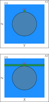 |
Fig. 1. Diagram illustrating the shape of the column taken from the original PSI model, considered in this work. The blue shaded area corresponds to the original PSI model. The green shaded area corresponds to the selected column. The red square shows the boundary of the CBP model. The black circle shows the boundary between the corona and the inner solar atmosphere. Upper panel: YZ plane at X = 0, with the X-direction corresponding to the LoS. Lower panel: XZ plane for Y = 0. Figure not to scale. |
We note that, through this approach, the contribution from the regions along the LoS between X ≃ −0.023 R⊙ to X ≃ 0.023 R⊙ is counted twice, once for each model. Regardless, this approach avoids the discontinuities in the magnetic field that would be introduced if the two models were merged while removing the part of the PSI section that coincides with the CBP model in the X direction. Moreover, we verified that the contribution to the overall intensity from the overlapping region of either of the PSI models is not appreciable at the plot level, for any of the considered lines. The intensity and polarization signals obtained by accounting for the joint contributions from the CBP and PSI models are shown and discussed in Sect. 4, after presenting the results of the CBP model alone in Sect. 3.
2.3. Simplifying assumptions
For the calculations presented in this work, we made several assumptions that considerably reduced their computational cost. First, P-CORONA allows for the option of imposing the Hanle saturation limit in the SEE. As noted in Sect. 1, this assumption can safely be made for the forbidden lines considered in this work. In addition, because the considered input radiation field corresponds to the photospheric continuum, it is essentially flat in the spectral vicinity of each of the considered lines. Thus, the effects of Doppler brightening or dimming should not be expected to play any role, and their influence can be neglected in the SEE, allowing for a further decrease in computational cost.
The atomic models considered for the calculations were obtained from the CHIANTI database (version 10.1; see Dere et al. 2023), but the total number of levels had to be limited for computational feasibility. As shown in Schad & Dima (2020), for the four considered lines, the relative difference between the emission obtained from CHIANTI by considering the largest possible atomic models and by considering only the lowest 100 levels does not exceed 5%, even within the electron density ranges for which the discrepancy is the largest (but see also the recently published work by Del Zanna & Supriya 2025, which presents a reduced 55 level model for modeling the Fe XIII infrared forbidden lines). In the present work, we applied P-CORONA to the CBP model, comparing the  ,
,  , and PL signals obtained when changing the number of levels considered in the corresponding atomic models, taking the 200 level case as a benchmark. Because of the high computational demands of such tests, we carried out the required calculations by first reducing the spatial resolution of the CBP model from 5123 points to 1513 through linear interpolation. Compared to the benchmark, the atomic models with 31 levels yield lower
  values, but by at most 5% for Fe5303, and by less that 3% for the other considered lines. The
  signals vary by less than 1% for any of the considered lines when taking only 31 levels, compared to the benchmark case. Although the relative variations of PL in the 31 level case are more significant, with local increases of over 20% with respect to the benchmark being found for Fe10747, such variations are found precisely where the linear polarization amplitude is lowest. We verified that such considerations do not affect the qualitative results shown in the following sections. Thus, the synthetic intensity and polarization signals shown in the following sections were calculated by taking only the lowest 31 levels for each atomic model.
3. Synthesis at a typical instant in the CBP evolution
We first focused on the results of the P-CORONA synthesis for Fe10747, carried out for the CBP model described in Sect. 2.2.1 (corresponding to an instant 201.7 minutes from the start of the simulation). The fan-spine magnetic topology of this model is illustrated in the left panel of Figure 2. The image shows a number of magnetic field lines (in red) traced from the neighborhood of a null point that delineate the fan surface (field lines going toward the horizontal boundaries of the domain) and the upper and lower spine (field lines that go toward the top and bottom of the domain). The wavelength-integrated intensity  (upper right panel),
  (lower central panel), and PL (lower right panel) calculated with P-CORONA are shown in the same figure. For reference, we also show the intensity mimicking a limb observation by SDO/AIA in the 193 Å channel (upper central panel), computed with CHIANTI (Dere et al. 2023). For this panel, we used the spatial coordinates taken directly from the numerical CBP model, rather than those corresponding to the input for P-CORONA (as in the rest of the figures shown in this work). The two coordinate systems are related through a 90° rotation with respect to the z-axis and a unit conversion to R⊙, corresponding to 695.7 Mm, while also considering that z = 0 Mm corresponds to Z = R⊙.
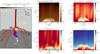 |
Fig. 2. CBP model corresponding to 201.7 minutes from the start of the Bifrost simulation originally presented in Nóbrega-Siverio et al. (2023), and associated spectral synthesis calculations. Left panel: Magnetic topology of the CBP model (red lines), superimposed on a horizontal map of Bz at z = 0. The red-green-blue coordinate system of the Bifrost model indicates the x, y, z axes. Upper central panel: Synthetic intensity computed with CHIANTI (Dere et al. 2023), mimicking a limb observation by SDO/AIA 193 Å. The rest of the panels correspond to synthetic quantities of Fe10747 line, obtained with P-CORONA. Upper right panel: Wavelength-integrated intensity |


For the  signal of Fe10747, there is a clear enhancement within the CBP region, which is mostly contained less than 0.01 R⊙ from the base of the corona. In the considered CBP model, the temperature and electron density are appreciably higher underneath the fan surface, leading to enhanced emission and thus the observed brightening. Within the CBP region, the
  signals reach values well above 0.1%, and could thus be expected to be detectable with future coronagraphs whose polarimetric sensitivity and resolution is comparable to that of Cryo-NIRSP/DKIST but which can observe closer to the base of the corona. Interestingly, we verified that, throughout the PoS, the
  signals are in good agreement with the ratio of the maximum V over the maximum I in the spectral vicinity of the line (i.e., |Vmax|/Imax).
The linear polarization, on the other hand, reaches its largest amplitudes outside the CBP. At 0.02 R⊙ above the base of the corona, the PL amplitude is on the order of 1%, but it is strongly suppressed within the CBP region, where it drops below 0.1% and often even below 0.01%. We recall that both collisional and radiative processes contribute to the excitation of the upper level of the transition but, assuming isotropic collisions, only the absorption of anisotropic radiation leads to atomicpolarization in the upper level of the line transition and, thus, to linear polarization. The aforementioned enhanced electron density within the CBP region does not only induce an increased intensity brightening; it additionally causes a higher rate of collisional excitations, leading to cascades that further populate the upper level, and a higher rate of collisional depolarization. As a result, the atomic polarization of the upper level decreases and, consequently, PL is also reduced (for a discussion on the impact of collisions on the atomic alignment in high-density regions of the corona, see Schad & Dima 2020). We verified that the linear polarization amplitude would be even lower within the CBP (decreasing further by up to 20%) if 200 levels were taken for the atomic model instead of 31.
The calculations for the other three lines investigated in this work are shown in Figure 3. The four lines can be ordered according to their intensity within the CBP, from brightest to darkest, as Fe5303, Fe10747, Si14301, and Si39343 (we note that, in the figures, the intensity scale is adjusted for each considered line). We find the same ordering, from highest to lowest, for their peak response temperature and for the Einstein coefficients for spontaneous emission (see Table 1). On the other hand, outside the CBP region, the highest intensity is found for Si14301, which has a peak emission around T = 106.15 K or 1.4 MK, whereas significantly lower intensities are found for the other lines. The contrast between the intensity within the CBP and outside it is particularly low for the Si39343 line, whose peak emission falls at around T = 106.05 K, or 1.1 MK.
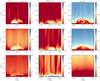 |
Fig. 3. Wavelength-integrated profiles obtained from P-CORONA calculations for the CBP model at 201.7 minutes from the start of the simulation. Left, central, and right columns show the quantities |


Regarding the  signals in the CBP, we find the highest amplitudes for Si39343, with intermediate amplitudes for Fe10747 and Si14301, and the lowest for Fe5303. However, even for the latter line, these signals often approach 0.1%. The differences between the lines could be expected from the fact that the circular polarization patterns arise from the Zeeman effect, whose amplitude scales with the wavelength of the considered line. As for the linear polarization, we find the PL amplitudes to be highest for Fe10747, followed by Si14301, Fe5303, and lowest for Si39343 (in agreement with the results of Judge et al. 2006, which correspond to calculations at 0.07 R⊙ above the solar limb using an idealized, spherically symmetric, hydrostatic, and isothermal coronal model). For all lines, the PL is strongly suppressed within the CBP, for the reasons explained above. Thus, we consider the linear polarization to be of limited utility for diagnostics of the magnetic fields in the low-corona CBP regions. Nevertheless, for completeness, we show in Appendix A the linear polarization angles (defined as in Equation (2)) associated with the calculations presented in this section.
4. Coronal material along the line of sight
We also analyzed how the intensity and polarization patterns are modified in the more realistic scenario of accounting for the coronal material lying along the LoS, beyond the spatial domain of the CBP model (which extends little more than 30 Mm, or 0.045 R⊙, in any spatial direction). We considered the impact of models PSI1 and PSI2 introduced in Sect. 2.2.2, which extend from −3 R⊙ to 3 R⊙ in the LoS direction, for the four forbidden lines considered in this work. Model PSI1 can be considered to represent a coronal hole, and its temperature is slightly lower than that of model PSI2: their average temperature is 1.07 MK and 1.15 MK, respectively, whereas their average electron density is 2.8 ⋅ 107 cm−3 and 2.9 ⋅ 107 cm−3, respectively. Particularly for the case of the lines with a high peak response temperature, we verified that PSI1 presents a substantially loweremission integrated along the LoS than model PSI2. For instance, for the Fe10747 line, the integrated emission is more than one order of magnitude lower, which is in rough agreement with the difference in the contribution functions of the line at 1.07 and 1.15 MK (e.g., Figure 2 of Schad & Dima 2020). To compare the role played by temperature and electron density in the resulting emission, we verified that artificially increasing the temperature by 25% at all spatial points of the PSI1 model increases the resulting emission by roughly a factor of 10, whereas the same increase in density leads to more moderate increase in emission, of roughly 40%.
For the four lines of interest, the  ,
,  , and PL signals obtained when considering the CBP model together with either PSI1 or PSI2 are shown in Figures 4 and 5, respectively. We begin the discussion by focusing on the impact of the PSI models on the Fe10747 line, which corresponds to the upper row of the figures, and compare them to the calculations considering the CBP model alone, shown in Figure 2. In intensity, we find that the contribution from PSI1 does not appreciably impact the signal from the CBP region, although it is certainly noticeable outside it. On the other hand, the contribution from model PSI2 has a strong impact on the intensity signal both outside the CBP and within it. We find a similar impact on the
  signals; inside the CBP region, the circular polarization amplitude is barely affected by PSI1, but it is greatly reduced when including instead the contribution from PSI2. The magnetic fields in PSI1 and PSI2 have strengths of ∼1 G, which is substantially lower than the ones found in the high-density regions of the CBP model. Because of their relatively low magnetic field strength, when the PSI models contribute significantly to the amplitude of the intensity profile, they do not proportionally enhance the amplitude of the Stokes V profile, which is produced by the Zeeman effect. Thus, a substantial contribution from the PSI models to
  results in a net decrease of
  .
.
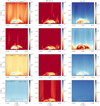 |
Fig. 4. Synthetic signals obtained by P-CORONA, for the radiation emitted by both the CBP and model PSI1 (see text), representative of the surrounding coronal material along the line of sight. Left, central, and right columns show the quantities |


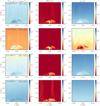 |
Fig. 5. Synthetic signals obtained by P-CORONA, for the radiation emitted by both the CBP and model PSI2 (see text), representative of the surrounding coronal material along the line of sight. Left, central, and right columns show the quantities |


The linear polarization signals of the Fe10747 line are far more vulnerable to the contribution from the surrounding material, which appreciably enhances the amplitude of the resulting PL signals in the CBP region, even for the PSI1 model. The electron density of this material is lower than that of the plasma underneath the CBP fan surface. Because of this, even if the emission is comparatively low, the relative contribution from scattering processes increases, leading to a larger linear polarization amplitude. Moreover, because the surrounding material is farther from the base of the corona than the CBP, the radiation reaching it from the photosphere is more anisotropic, further contributing to the scattering polarization amplitude. For instance, when considering PSI2, we verified numerically that most of the contribution to the overall PL comes from the points along the LoS between roughly 0.2 and 0.4 solar radii from the base of the corona, where the anisotropy of the radiation increases substantially, compared to its value below 0.1 solar radii (e.g., Li et al. 2017).
By comparing Figures 3, 4, and 5, we can evaluate the impact of the PSI models on the other forbidden lines under investigation. Regarding the intensity, we observe that the coronal material from these models has the smallest impact on the signals of Fe5303, whose peak response temperature is the highest, at ∼106.3 K (see Table 1). The contribution from PSI1 has no appreciable impact on the intensity, even outside the CBP. When considering the contribution from PSI2, we do find an enhancement outside the CBP, although the signal within it remains largely unaffected. As for Si14301, the contribution from PSI1 clearly impacts the intensity both inside and outside the CBP, slightly more so than for the case of Fe10747. Model PSI2 has a far stronger impact, to the point that the CBP is barely distinguishable from the background coronal intensity. For the case of Si39343, which has the lowest peak response temperature, the CBP signal is completely drowned out by the contribution of the surrounding coronal material, whether model PSI1 or PSI2 is considered.
For the cases presented in this section, we find that the  signals within the CBP region are generally impacted by the contribution from the PSI models to a similar degree as the
  signals. We expect that, if a CBP can clearly be observed in the intensity signals of a given line, the detected circular polarization patterns can be mainly attributed to the emission from the CBP region.
Regarding the linear polarization fraction, the findings for the Si14301 and Si39343 lines are similar to those for Fe10747: the PL signals in the CBP are strongly affected even in cases where the  signals are not. For the Fe5303 line, on the other hand, the contribution from PSI1 or PSI2 is so low, compared to that from the CBP, that the PL signals are only slightly affected even when considering PSI2, and thus their amplitude remains small. These results reinforce the conclusion that the linear polarization signals of these lines are not suitable diagnostics for the magnetic field in the CBP region.
5. Applicability of the weak field approximation
For the present section we analyzed the suitability of the circular polarization signals for inferences of the longitudinal component of the magnetic field within the regions that emit in the considered forbidden lines. The circular polarization patterns presented above are due to the energy shift between different sublevels of the same J level, induced by the magnetic field (i.e., the Zeeman effect). The LoS component of the magnetic field can be inferred by making use of the weak field approximation (WFA), through which the circular polarization can be related to the wavelength derivative of the intensity profile according to (e.g., Trujillo Bueno & del Pino Alemán 2022)
 (3)
(3)
where geff is the (dimensionless) effective Landé factor of the transition, λ0 is the wavelength of the considered line transition in Å, and BLOS is the LoS component of the magnetic field in G. The partial derivative with respect to λ is also given in Å units. As noted by Casini & Judge (1999), this relation should also contain a correction factor due to the atomic alignment of the upper level of the line. However, within the CBP, the atomic alignment should be very small, as a consequence of the relatively high density and predominance of collisional processes (discussed in Sect. 3). On this basis, the corresponding correction factor is neglected in the present work. The application of the WFA hinges on a few assumptions, notably that the magnetic splitting must be much smaller than the Doppler width of the lines (which is valid for the conditions for the coronal lines considered in this work). It also requires the longitudinal component of the magnetic field to be constant within the emitting medium. Such an assumption is not guaranteed in the considered atmospheric model, and its influence must be examined.
Given the I(λ) and V(λ) profiles, we can use Equation 3 to infer the average LoS component of the magnetic field (i.e., BLOSWFA) through least-squares minimization. We begin the discussion focusing on the Fe10747 line (Figure 6, upper row). The upper left panel shows the magnetic field inferred when applying the WFA to the profiles obtained for the CBP model using P-CORONA (corresponding to the calculations whose resulting wavelength-integrated signals are shown in Figure 2). The least-squares minimization was computed taking the wavelength grid points provided by P-CORONA within a range of 6 Å, centered at the wavelength of the transition. Within the CBP, we find both positive and negative longitudinal magnetic fields (i.e., pointing towards and away from the observer, respectively), with strength exceeding 50 G, which is significantly higher than outside of it. We note that this approach gives information on the magnetic field within the regions from which the line’s radiation is emitted.
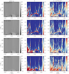 |
Fig. 6. Quantities resulting from application of the WFA. From top to bottom, the four rows show the quantities for the Fe10747, Fe5303, Si14301, and Si39343 lines. Left column: Line-of-sight magnetic fields, inferred through the application of the WFA to the synthetic profiles obtained from P-CORONA (see text). Central column: Pearson coefficient for the correlation between the V(λ) and ∂I(λ)/∂λ synthetic profiles, at each point on the PoS. Right column: Square relative error between the V(λ) profiles resulting from the synthesis and from the application of the WFA. |
The circular polarization patterns shown, for instance, in Figure 2, do not originate from a localized source. Instead, they are emitted from an extended spatial range, along which the thermodynamic properties including BLOS may vary, thus compromising the applicability of the WFA. As a result, the V(λ) profile may not be proportional to ∂I(λ)/∂λ. The upper central panel of Figure 6 shows, for each pixel on the PoS, the Pearson correlation coefficient between the two profiles of the Fe10747 line, taking the same wavelength range as for the least-squares minimization. A value of unity would thus indicate perfect correlation and zero indicates that they are completely uncorrelated quantities. Within much of the CBP, the coefficient is close to unity, but it tends to fall below 0.6 (indicating a low correlation) close to the regions on the PoS where there is a change in sign in BLOS or it otherwise becomes small. In addition, we computed the square error as
where Vcalc is the circular polarization computed using P-CORONA and VWFA is obtained according to Equation (3), taking the derivative of the intensity from the P-CORONA calculation and using the value of BLOS found through a least-squares minimization. The sum over i encompasses the same spectral grid points as for the least-squares minimization. We find that, within the CBP, the square error is largest where the Pearson coefficient becomes smallest. Again, this coincides with the regions on the PoS where the inferred BLOS is small.
As a further test of the suitability of the inference of the LoS magnetic field using the WFA, we calculated the average BLOS in the LoS direction directly from the values of the numerical CBP model. We performed the averages by weighting the magnetic field at each spatial point by the emissivity in the considered spectral line ϵI, computed as a function of temperature, electron density and distance from the solar surface using CHIANTI as
 (4)
(4)
where we recall that x is the LoS direction, and thus Bx is equivalent to BLOS in the CBP model. We focus first on the Fe10747 line; the resulting average is shown in the upper left panel of Figure 7. A visual comparison between this quantity and the LoS component of the magnetic field as inferred from the WFA (see upper left panel of Figure 6) shows a generally good agreement. This comparison is shown directly in the upper central panel of Figure 7, in terms of the departure from unity of the ratio between the absolute value of the two quantities. In most of the CBP region, the two quantities deviate by less than 5%, although discrepancies as large as 30% can be found coinciding with the regions with a low correlation coefficient between Vcalc and VWFA. This generally good agreement is consistent with the findings of Schad & Dima (2020), who performed calculations using the PyCELP code and a MURaM simulation from Rempel (2017). That model is representative of a relatively simple bipolar active region and yielded substantially weaker longitudinal magnetic fields. As suggested by those authors, the remarkable agreement between the two quantities is due to the fact that the WFA gives more weight to the regions along the LoS where most of the emission occurs in the considered line.
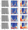 |
Fig. 7. Quantities for the WFA analysis, taken from the values of the numerical CBP model. From top to bottom, the four rows show the corresponding quantities when considering the Fe10747, Fe5303, Si14301, and Si39343 lines. Left column: Spatial average along the LoS direction of BLOS, weighted by the emission of the considered line as computed by CHIANTI. Central column: Departure from unity of the ratio between the BLOS inferred from the WFA and the average BLOS of the atmospheric model, weighted by the emission. Right column: Measure of the cancellation of BLOS along the LoS given as the ratio of the integral quantities | < Bx, ϵI > | over < |Bx|,ϵI> (see text). |
To further illustrate this point, we show in Figure 8 the quantity < Bx > = ∫Bx dx, whose value is very different from that of < Bx, ϵI>. The former is predominantly positive within the CBP, whereas the latter shows distinct regions with positive and negative sign. The values of < Bx> are substantially lower than those of < Bx, ϵI>, suggesting that relatively strong magnetic fields are present in the high-temperature regions of the CBP where the emission occurs. In addition, we computed the ratio  , or, using the symbol defined in Equation (4), | < Bx, ϵI > | over < |Bx|,ϵI>. This quantity gives a measure of the magnetic field cancellations along the LoS, while giving more weight to the spatial regions where the emissivity is strongest. If the magnetic field had the same sign along the integration domain, then the numerator and the denominator would have the same value and the ratio would be unity. Conversely, if the sign were to change in such a manner that the emission-weighted magnetic fields perfectly cancel along the LoS, the resulting quantity would be zero. This ratio, for the same CBP model and considering the Fe10747 line, is shown in the upper right panel of Figure 7. The regions with the greatest cancellation along the LoS coincide with those with the highest discrepancy between the magnetic fields inferred through the WFA and those resulting from the average over the model itself, and where the correlation coefficients are lowest.
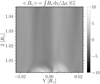 |
Fig. 8. Spatial average, along the LoS direction, of the LoS component of the magnetic field, BLOS, as taken from the Bifrost CBP model discussed in the main text. |
We now present the same analysis for the other lines, showing the corresponding quantities in Figures 6 and 7 in the second, third, and fourth rows, for Fe5303, Si14301, and Si39343, respectively. When applying the least-squares minimization for the WFA, we took a 6 Å spectral interval for the Fe5303 and a 10 Å interval for both Si14301 and Si39434. For Fe5303, we obtained BLOSWFA values that are similar to those obtained when considering the Fe10747 line. The results for the associated quantities are also very similar; the correlation coefficient (central column of Figure 6) and the departure from unity of the ratio between BLOSWFA and < Bx, ϵI> (central column of Figure 7) both show their lowest (i.e., worst) values in the same regions on the PoS where BLOS has its lowest values. These regions also tend to coincide with the regions where the square error (right column of Figure 6) is the largest and for which the strongest cancellations occur, as indicated by low values of  (right column of Figure 7).
On the other hand, the qualitative differences are more considerable for the results of the Si14301, and even more so for the Si39343 line. There is a clear increase in the area on the PoS where the discrepancy between BLOSWFA and < Bx, ϵI> is large (> 25%), where the Pearson coefficient falls below 0.6, and where the square error E is large. Again, these regions coincide with those where there are large cancellations of the magnetic field along the LoS. Significantly lower magnetic fields are found when applying the WFA to these lines. Because these lines have a lower peak response temperature, they are emitted over a more extended region within the CBP than in the case of the Fe10747 and Fe5303 lines. As a result, when considering the integration of BLOS along the LoS, weighted by the emissivity, cancellations occur more frequently.
The investigations presented in this section were carried out considering the profiles obtained when considering only the CBP model. However, as noted in Sect. 4, when the contribution from the surrounding material significantly impacts the intensity signal in the CBP, it should be expected to also impact the  signal. This, in turn, would cause the BLOS inferred via the WFA to be underestimated. We evaluated the impact on the
  inferred within the CBP region, although the corresponding figures are not shown for the sake of brevity. In the case of Fe5303, the field strength is underestimated by less than 5% within most of the CBP when considering PSI1 and by less than 20% when considering PSI2. For Fe10747, the underestimation is generally less than 15% when considering PSI1, but it approaches or exceeds 80% in most of the CBP region for PSI2. For Si14301, the decrease in the inferred BLOS is appreciably greater than for the case of Fe10747 for either of the PSI models. For Si39343, in agreement with the results shown in Figures 4 and 5, the contribution from the surrounding material strongly contaminates the CBP signal whether PSI1 or PSI2 is considered, rendering the WFA inapplicable.
We thus regard Fe10747 and Fe5303 as the most suitable lines for the application of the WFA. Moreover, the circular polarization amplitude, normalized to intensity, is significantly larger for Fe10747 than for Fe5303 within the CBP region thanks to the former’s longer wavelength. Because of this, we focus on the Fe10747 line in the following section.
6. Evolution over time
Even state-of-the-art coronagraphs such as Cryo-NIRSP/DKIST require exposure times of tens of minutes to achieve a signal-to-noise ratio (S/N) that allows V/I signals in the Fe10747 line with amplitudes of around 0.1% to be measured (e.g., Schad et al. 2024). In the present section, we investigate how the signals of this line change when accounting for the evolution of the CBP and averaging over time spans of tens of minutes, rather than considering the signals at specific instants as was done in the previous sections. Thus, we consider the CBP model discussed in Sect. 2.2 at several instants between t = 185 and 218.3 min, corresponding to a total interval of 33.3 minutes or 2000 seconds. To obtain the time-averaged signals, we summed the Stokes profiles obtained with P-CORONA from the CBP model with a cadence of 100 s and divided by the total time interval4. The resulting average  ,
,  , and PL signals is shown in Figure 9. An animation showing the corresponding quantities for different instants in time increments of 100 seconds can be found in the online material.
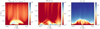 |
Fig. 9. Time average for the Fe10747 line resulting from syntheses taking the CBP model at instants of the simulation between 185 and 218.3 minutes, with 100-second cadence. An animated figure showing the results of those calculations is available online. The panels correspond to the same quantities as in Figure 2. |
The left panel of the figure shows the average  signals, in which one can see that the signatures are somewhat smeared due to the time evolution compared to the results at a given instant (see Figure 2), both within the CBP and outside it. Nevertheless, the CBP itself is still clearly appreciable, and is brighter than the surrounding region by about an order of magnitude. The
  image, shown in the central panel, is also somewhat smeared by the time evolution: there is an appreciable decrease both in the maximum amplitude and in the area within the CBP where the amplitude exceeds 0.1%. Regardless, the area where the amplitude is above 0.1% remains considerable.
As can be seen in the right panel of the figure, the amplitude of the linear polarization increases within the CBP, compared to the polarization at a single instant (see Figure 2). This is because there are instants during the evolution in which, for a given point on the PoS within the CBP region, the density is comparatively low throughout the LoS, thus contributing to a higher PL. However, for the case of Fe10747, this contribution would still be drowned out by the external coronal material lying on the LoS, as discussed in Sect. 4.
We also analyzed the information on the magnetic field that can be accessed from the circular polarization signals through the WFA (see Sect. 5). The analogous quantities to those corresponding to the Fe10747 line in Figures 6 and 7, but for the time-averaged signals, are shown in Figure 10. The magnetic fields inferred from the WFA, BLOSWFA (upper left panel), are compared to the emission-weighted fields of the model averaged over the LoS, < Bx, ϵI> (lower left panel), for which we also averaged over the results at different instants in the evolution of the CBP simulation. The two values show a reasonably good agreement within the CBP. Compared to the results when considering a single instant in time (see Sect. 5), the time-averaged values of < Bx, ϵI> show a noticeable decrease in the average magnitude and a predominance of negative BLOS. The decrease in the average magnitude within the CBP is an expected consequence of the change in orientation of the magnetic field within the considered time interval. Similarly to the two distinct regions with positive and negative sign found when considering the instant at 201.7 minutes, we attribute the preponderance of a negative sign of BLOSWFA in the CBP to the particular orientation of the magnetic field in the region along the LoS within the strongest emission.
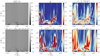 |
Fig. 10. Quantities for the WFA analysis, accounting for the time evolution of the CBP. Upper and lower rows: Each panel shows the same quantities as in the corresponding columns of Figs. 6 and 7, respectively. Here the quantities are shown for Fe10747, but having integrated over the instants of the CBP model between 185 and 218.33 minutes (see text). |
Regarding the departure from unity of the ratio of BLOSWFA to < Bx, ϵI> (lower central panel), we find patches within the CBP region where the discrepancies exceed 30% which, similarly to what was discussed in Sect. 5, tend to coincide with those regions where the inferred magnetic field is weakest. As expected, such regions also tend to coincide with those where the Pearson coefficient (upper central panel) is lowest, the square error E (upper right panel) is largest, and the most cancellations of the emission-weighted LoS occur (lower right panel). Thus, although the circular polarization amplitude in the CBP is somewhat attenuated when accounting for roughly 30 minutes of evolution in the CBP, it can still provide measurable and useful information about the LoS magnetic fields within the higher-temperature regions of the structure from which Fe10747 is emitted.
7. Conclusions
The advent of the new generation of coronagraphs, both in space-based missions such as VELC/Aditya-L1 (see Singh et al. 2019) and large-aperture ground-based facilities such as Cryo-NIRSP/DKIST (Rimmele et al. 2020; Fehlmann et al. 2023), has renewed the interest in studying the intensity and polarization of forbidden spectral lines for diagnostics of coronal magnetic fields. Here we studied the suitability of a selection of forbidden lines for magnetic diagnostics of fundamental structures in the lower solar corona, specifically CBPs. We focused on four forbidden lines: Fe10747, Fe5303, Si14301, and Si39343.
We computed the intensity and polarization patterns of the forbidden lines under investigation, considering a model representative of a CBP within a coronal hole, obtained from the Bifrost simulation presented in Nóbrega-Siverio et al. (2023). The synthetic signals were calculated using the publicly available P-CORONA code (Supriya et al. 2025), which accounts for collisional and radiative processes, scattering polarization, and the impact of the magnetic field through the Hanle and Zeeman effect. For the calculations we considered the magnetic fields to be in the Hanle saturation regime. For all four considered lines, we used atomic models whose size was limited to 31 levels, after verifying the suitability of these models for investigations of CBPs using a reduced-resolution atmospheric model for computational feasibility.
We first focused on a typical instant in the evolution of the CBP, corresponding to 201.7 minutes from the start of the simulation, and computed the Stokes profiles. As expected, for all four considered lines, the wavelength-integrated intensity images showed a clear brightening in the CBP region, which extends for some 8 Mm, or a little in excess of 0.01 R⊙ from the base of the corona. The contrast with the fainter intensity emitted from outside the CBP is especially apparent for the lines with the highest peak response temperature – namely Fe5303 and Fe10747 – and is much more modest for Si39343, which has the lowest. The circular polarization signals, displayed as  , have their largest amplitude within the CBP where, for the four considered lines, they approach or exceed 0.1%, and could be possibly detected using large-aperture coronagraphs with capabilities similar to Cryo-NIRSP/DKIST, but which can observe below 0.05 R⊙ from the base of the corona.
The linear polarization signals, on the other hand, are found to be large outside the CBP region (where their amplitude exceeds ∼1%), but they drop precipitously within the CBP, generally falling well below 0.1%. Underneath the fan surface, where the electron density can reach 109.5 cm−3, collisional processes dominate over radiative ones, reducing the relative contribution of scattering polarization.
The radiation emitted from the CBP reaches the observer together with the radiation emitted by the enveloping corona along the LoS. To account for this, we added the synthetic profiles resulting from the CBP model to those resulting from models representative of the outer coronal material, extending from −3 R⊙ to 3 R⊙ in the LoS direction. To that end, we used coronal models based on the data provided by Predictive Science, Inc. We extracted columns from this model that have the same PoS dimensions as the CBP model and are tangent to the base of the corona. We carried out calculations for two distinct models, PSI1 and PSI2, with the former having a slightly lower average temperature and a significantly lower emission in the four considered lines. The contribution from the surrounding material, relative to the intensity signal from the CBP, depends both on the peak response temperature of the considered line and on the considered PSI model. For the Fe5303 line, even PSI2 gives only a modest contribution to its signal, due to its high peak response temperature. For Fe10747, PSI1 does not have a significant impact on the intensity from the CBP which, by contrast, is drowned out when considering PSI2. Similar results were found for Si14301, although the contribution from the PSI1 model has a slightly greater impact on the CBP signals. The Si39343 signals are completely dominated by the contribution from either model, PSI1 or PSI2.
We find that the  signals are impacted by the surrounding material to a similar degree as the intensity. This suggests that if the CBP can be clearly observed in intensity, most of the circular polarization should be emitted from that structure. On the other hand, the contribution of the outer coronal material tends to substantially impact the linear polarization amplitude from the CBP for all the considered lines except Fe5303 (which has a peak response at 2 MK). However, in this case, the linear polarization in the CBP region is quite small, being mostly below 0.1% and often on the order of 0.01%. The suitability of the linear polarization signals for magnetic diagnostics of CBPs or similar low-corona structures with a large electron density may thus be easily compromised by both their relatively small amplitude and the contribution from external coronal material along the LoS.
We also analyzed the application of the WFA to the synthetic intensity and circular polarization signals resulting from the CBP model. We recall that the WFA mainly provides information about the magnetic field in the intervals along the LoS where the emission is highest for the considered lines. The inferred BLOSWFA is significantly stronger than the average within the CBP box, unless we weight the average with the line emissivity along the LoS (i.e., < Bx, ϵI> ). The latter quantity is in good agreement with the inferred BLOSWFA at the regions on the PoS, corresponding to the CBP, where the Pearson correlation coefficient between V(λ) and ∂I/∂λ is high. Such regions coincide with those for which there are no significant cancellations of BLOS, in the intervals along the LoS where the emission is high. They are more abundant when considering lines with a higher peak response temperature, most likely because the radiation is mainly emitted from a narrower spatial region and is thus subject to fewer cancellations. Unsurprisingly, the regions with significant cancellations tend to coincide with the regions with a small inferred BLOS.
The ideal data set to study the CBP magnetic fields should thus present a strong intensity contrast between the CBP itself and the rest of the coronal material, indicating that the CBP supplies the dominant contribution to the observed signal. This would most likely be found in or around a coronal hole. As for the circular polarization, the most useful profiles would be those with a high correlation with the wavelength derivative of the intensity, typically occurring when there is no magnetic cancellation along the LoS; in those cases one should expect that the WFA can be suitably applied.
Finally, we studied how the signals of the Fe10747 line change due to the time evolution of the CBP. We averaged the signals obtained at different instants of the simulation at a 100 s cadence and over an interval of ∼30 minutes which, when observing the Fe10747 line with large-aperture telescopes, would provide a S/N high enough to suitably measure polarization signals of about 0.1%. The resulting time-averaged signals remain suitable for the application of the WFA: the CBP is still clearly appreciable in intensity, even though the contrast with the surrounding coronal material is somewhat reduced, and there is still a reasonably good agreement between the BLOS inferred by the WFA and the models’ emission-weighted BLOS averaged along the LoS.
The analysis carried out in this paper is particularly relevant for understanding the polarization signals in systems composed of coronal loops, like the CBPs, which are ubiquitous structures in the solar corona. Of the four forbidden lines we investigated, we consider Fe5303 and Fe10747 to be the most suitable for diagnosing CBP magnetic fields. These lines are less affected by contributions from the surrounding coronal material and produce the most accurate results when applying the WFA. This is particularly interesting given that CBPs typically exhibit temperatures between 1.0 and 3.4 MK (e.g., Kariyappa et al. 2011; Madjarska 2019). In such temperature ranges, the hotter lines tend to show higher contrast relative to the ambient corona, especially when the CBP is located within a coronal hole or in the quiet Sun – as is typically the case. Therefore, although our conclusions are based on a numerical model, they likely hold in real solar conditions and may be applicable more broadly. In addition, our results can provide valuable insights for future missions aiming to perform spectropolarimetric observations of structures in the very low corona.
Data availability
Movie associated with Figures 9 and B.1 is available at https://www.aanda.org.
These temperatures are largely determined by the ionization fraction of the relevant chemical species, whereas the population of the line’s upper level relative to that of the ion varies much more slowly with temperature.
These abundances are lower than the ones obtained when accounting for first ionization potential (FIP) effects (e.g., Laming 2015). Accounting for such increased abundances should not be expected to substantially affect the polarization fraction of the considered lines, but could enhance their intensity.
We also considered averages with lower cadences, and found no change in the resulting quantities. We thus expect that calculations at higher cadences would not yield different results.
Acknowledgments
This research was supported by the European Research Council through the Synergy grant No. 810218 (“The Whole Sun” ERC-2018-SyG). This project also benefited from discussions that took place at the “Whole Sun Meetings” supported by the same grant. E.A.B. and S.H.D. acknowledge support from the Agencia Estatal de Investigación del Ministerio de Ciencia, Innovación y Universidades (MCIU/AEI) under grant “Polarimetric Inference of Magnetic Fields” and the European Regional Development Fund (ERDF) with reference PID2022-136563NB-I00/10.13039/501100011033. D.N.S. acknowledges the computer resources at the MareNostrum supercomputing installation and the technical support provided by the Barcelona Supercomputing Center (BSC, RES-AECT-2021-1-0023, RES-AECT-2022-2-0002), as well as the resources provided by Sigma2 - the National Infrastructure for High Performance Computing and Data Storage in Norway. Prof. Trujillo Bueno’s careful reading of the manuscript and thoughtful comments are recognized with appreciation. Illuminating discussions with Drs. de Vicente, del Pino Alemán, and Shchukina are gratefully acknowledged. Valuable comments from the anonymous referee are sincerely appreciated.
References
- Allen, C. W. 2004, Allen’s Astrophysical Quantities (New York: Springer, New York) [Google Scholar]
- Arnaud, J. 1982, A&A, 112, 350 [Google Scholar]
- Casini, R., & Judge, P. G. 1999, ApJ, 522, 524 [NASA ADS] [CrossRef] [Google Scholar]
- Casini, R., & Judge, P. G. 2000, ApJ, 533, 574 [Google Scholar]
- Del Zanna, G., & Supriya, H. D. 2025, MNRAS, 537, 3781 [Google Scholar]
- Dere, K. P., Del Zanna, G., Young, P. R., & Landi, E. 2023, ApJS, 268, 52 [NASA ADS] [CrossRef] [Google Scholar]
- Dima, G. I., Kuhn, J. R., & Schad, T. A. 2019, ApJ, 877, 144 [Google Scholar]
- Eddy, J. A., & McKim Malville, J. 1967, ApJ, 150, 289 [Google Scholar]
- Fehlmann, A., Kuhn, J. R., Schad, T. A., et al. 2023, Sol. Phys., 298, 5 [Google Scholar]
- Gao, Y., Tian, H., Van Doorsselaere, T., & Chen, Y. 2022, ApJ, 930, 55 [NASA ADS] [CrossRef] [Google Scholar]
- Gibson, S., Kucera, T., White, S., et al. 2016, Front. Astron. Space Sci., 3, 8 [NASA ADS] [CrossRef] [Google Scholar]
- Green, L. M., Török, T., Vršnak, B., Manchester, W., & Veronig, A. 2018, Space Sci. Rev., 214, 46 [Google Scholar]
- Gudiksen, B. V., Carlsson, M., Hansteen, V. H., et al. 2011, A&A, 531, A154 [NASA ADS] [CrossRef] [EDP Sciences] [Google Scholar]
- Jarolim, R., Thalmann, J. K., Veronig, A. M., & Podladchikova, T. 2023, Nat. Astron., 7, 1171 [NASA ADS] [CrossRef] [Google Scholar]
- Judge, P. G. 1998, ApJ, 500, 1009 [Google Scholar]
- Judge, P. G., & Ionson, J. A. 2024, The Problem of Coronal Heating (Cham: Springer) [Google Scholar]
- Judge, P. G., Low, B. C., & Casini, R. 2006, ApJ, 651, 1229 [Google Scholar]
- Kariyappa, R., Deluca, E. E., Saar, S. H., et al. 2011, A&A, 526, A78 [NASA ADS] [CrossRef] [EDP Sciences] [Google Scholar]
- Karna, N., Savcheva, A., Dalmasse, K., et al. 2019, ApJ, 883, 74 [Google Scholar]
- Khan, R., Gibson, S. E., Casini, R., & Nagaraju, K. 2024, ApJ, 971, 27 [Google Scholar]
- Kuhn, J. R., Coulter, R., Lin, H., & Mickey, D. L. 2003, in Innovative Telescopes and Instrumentation for Solar Astrophysics, eds. S. L. Keil, & S. V. Avakyan, SPIE Conf. Ser., 4853, 318 [Google Scholar]
- Laming, J. M. 2015, Liv. Rev. Sol. Phys., 12, 2 [Google Scholar]
- Landi Degl’Innocenti, E., & Landolfi, M. 2004, Polarization in Spectral Lines,, 307 (Dordrecht: Springer) [Google Scholar]
- Li, H., Landi Degl’Innocenti, E., & Qu, Z. 2017, ApJ, 838, 69 [Google Scholar]
- Lin, H., Kuhn, J. R., & Coulter, R. 2004, ApJ, 613, L177 [Google Scholar]
- Madjarska, M. S. 2019, Liv. Rev. Sol. Phys., 16, 2 [Google Scholar]
- Madjarska, M. S., Wiegelmann, T., Démoulin, P., & Galsgaard, K. 2024, A&A, 690, A242 [NASA ADS] [CrossRef] [EDP Sciences] [Google Scholar]
- Mickey, D. L. 1973, ApJ, 181, L19 [Google Scholar]
- Nóbrega-Siverio, D., Moreno-Insertis, F., Galsgaard, K., et al. 2023, ApJ, 958, L38 [CrossRef] [Google Scholar]
- Priest, E. 2014, Magnetohydrodynamics of the Sun (Cambridge University Press) [Google Scholar]
- Priest, E. R., Parnell, C. E., & Martin, S. F. 1994, ApJ, 427, 459 [Google Scholar]
- Raouafi, N. E., Patsourakos, S., Pariat, E., et al. 2016, Space Sci. Rev., 201, 1 [Google Scholar]
- Rempel, M. 2017, ApJ, 834, 10 [Google Scholar]
- Riley, P., Lionello, R., Linker, J. A., et al. 2011, Sol. Phys., 274, 361 [NASA ADS] [CrossRef] [Google Scholar]
- Rimmele, T. R., Warner, M., Keil, S. L., et al. 2020, Sol. Phys., 295, 172 [Google Scholar]
- Sahal-Brechot, S. 1974, A&A, 36, 355 [Google Scholar]
- Schad, T., & Dima, G. 2020, Sol. Phys., 295, 98 [Google Scholar]
- Schad, T., & Dima, G. 2021, Sol. Phys., 296, 166 [Google Scholar]
- Schad, T. A., Petrie, G. J. D., Kuhn, J. R., et al. 2024, Sci. Adv., 10, eadq1604 [NASA ADS] [CrossRef] [Google Scholar]
- Schmelz, J. T., Reames, D. V., von Steiger, R., & Basu, S. 2012, ApJ, 755, 33 [NASA ADS] [CrossRef] [Google Scholar]
- Singh, J., Prasad, B. R., Venkata, S., & Kumar, A. 2019, Adv. Space Res., 64, 1455 [Google Scholar]
- Supriya, H. D., Trujillo Bueno, J., de Vicente, Á., & del Pino Alemán, T. 2021, ApJ, 920, 140 [Google Scholar]
- Supriya, H. D., de Vicente, A., del Pino Alemán, T., Trujillo Bueno, J., & Shchukina, N. 2025, ApJ, 987, 39 [Google Scholar]
- Tomczyk, S., McIntosh, S. W., Keil, S. L., et al. 2007, Science, 317, 1192 [Google Scholar]
- Tomczyk, S., Card, G. L., Darnell, T., et al. 2008, Sol. Phys., 247, 411 [Google Scholar]
- Tomczyk, S., Landi, E., Berkey, B., et al. 2021, AGU Fall Meeting Abstracts, 2021, 2089 [Google Scholar]
- Trujillo Bueno, J. 2001, in Advanced Solar Polarimetry - Theory, Observation, and Instrumentation, ed. M. Sigwarth, ASP Conf. Ser., 161 [Google Scholar]
- Trujillo Bueno, J., & del Pino Alemán, T. 2022, ARA&A, 60, 415 [NASA ADS] [CrossRef] [Google Scholar]
- Warren, H. P., Crump, N. A., Ugarte-Urra, I., et al. 2018, ApJ, 860, 46 [Google Scholar]
Appendix A: Polarization angles
The four panels of Figure A.1 show the linear polarization angles α obtained when applying P-CORONA for the CBP model, for the Fe5303, Fe10747, Si14301, and Si39434 lines, respectively. They correspond to the same calculations that produced the  ,
,  and PL signals presented in Figures 2 (for Fe10747) and 3 (for the other lines). The linear polarization angle refers to the angle of the direction of largest linear polarization with respect to the Z-axis, with positive (negative) values representing a clockwise (counterclockwise) rotation of the plane of linear polarization (see Equation 2).
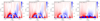 |
Fig. A.1. Linear polarization angle, with respect to the Z-axis, for the radiation emerging from the CBP. The four panels correspond to the values for Fe10747, Fe5303, Si14301, and Si39343 lines, respectively. The intensity and polarization were calculated with P-CORONA, using the CBP model at 201.7 minutes from the start of the simulation. The angles were obtained from the same calculations that yielded the results shown in Figures 2 and 3, for the corresponding spectral lines. |
Although the value of α near the edges of the box is slightly affected by the inclination between the vertical direction, Z, and the radial direction, this impact is very minor given the small size of the box. The variation in α is mainly due to the rotation in the plane of polarization induced by the magnetic field through the Hanle effect. We recall that the Hanle effect operates when the magnetic field is inclined with respect to the symmetry axis of the radiation field (in this case, the vertical). Moreover, for LoSs close to the limb, the direction of Hanle rotation depends on the sign of the LoS component of the magnetic field. However, in a manner analogous to what was discussed for the circular polarization in Sect. 5, the value of α does not simply provide a measure of the average longitudinal magnetic field along the LoS. The resulting signal gives more weight to regions where the emission in linear polarization (rather than intensity) is the strongest.
With this in mind, we now compare the α images for the four lines. Outside the CBP, we find the sign to be mostly negative, although there is some spatial fluctuation, especially for Fe5303. For the four lines, a plume-like structure with a positive sign is produced for Y > 0. Within the CBP, there are regions with both positive and negative signs, although with more spatial variability for the Fe5303 and Fe10747 lines, whose resulting α patterns are very similar. Finally, we highlight the sharp change in the sign for the Si39343 close to the base of the corona, which we attribute to the change in the sign of atomic polarization for electron densities around 108.5 cm−3 reported by Schad & Dima (2020).
Unfortunately, it must be stressed that the suitability for magnetic diagnostics of the linear polarization (including its angle) from the CBP is compromised by its relatively small amplitude and the contribution from the surrounding material. These drawbacks may be less of a concern for the linear polarization signals outside the CBP, but a more detailed analysis is beyond the scope of the present work.
Appendix B: Time evolution of the Fe10747 signals in the CBP
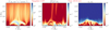 |
Fig. B.1. Animmation displaying the Fe10747 signals calculated with P-CORONA, as detailed in Sect. 2. The calculations were carried out using the CBP model introduced in Sect. 2.2.1, but at different instants between 183 and 218.3 minutes, in increments of ∼1.6 minutes (i.e., 100 seconds). Left panel: Wavelength-integrated intensity |


All Tables
All Figures
|
Fig. 1. Diagram illustrating the shape of the column taken from the original PSI model, considered in this work. The blue shaded area corresponds to the original PSI model. The green shaded area corresponds to the selected column. The red square shows the boundary of the CBP model. The black circle shows the boundary between the corona and the inner solar atmosphere. Upper panel: YZ plane at X = 0, with the X-direction corresponding to the LoS. Lower panel: XZ plane for Y = 0. Figure not to scale. |
| In the text | |
|
Fig. 2. CBP model corresponding to 201.7 minutes from the start of the Bifrost simulation originally presented in Nóbrega-Siverio et al. (2023), and associated spectral synthesis calculations. Left panel: Magnetic topology of the CBP model (red lines), superimposed on a horizontal map of Bz at z = 0. The red-green-blue coordinate system of the Bifrost model indicates the x, y, z axes. Upper central panel: Synthetic intensity computed with CHIANTI (Dere et al. 2023), mimicking a limb observation by SDO/AIA 193 Å. The rest of the panels correspond to synthetic quantities of Fe10747 line, obtained with P-CORONA. Upper right panel: Wavelength-integrated intensity |
| In the text | |
|
Fig. 3. Wavelength-integrated profiles obtained from P-CORONA calculations for the CBP model at 201.7 minutes from the start of the simulation. Left, central, and right columns show the quantities |
| In the text | |
|
Fig. 4. Synthetic signals obtained by P-CORONA, for the radiation emitted by both the CBP and model PSI1 (see text), representative of the surrounding coronal material along the line of sight. Left, central, and right columns show the quantities |
| In the text | |
|
Fig. 5. Synthetic signals obtained by P-CORONA, for the radiation emitted by both the CBP and model PSI2 (see text), representative of the surrounding coronal material along the line of sight. Left, central, and right columns show the quantities |
| In the text | |
|
Fig. 6. Quantities resulting from application of the WFA. From top to bottom, the four rows show the quantities for the Fe10747, Fe5303, Si14301, and Si39343 lines. Left column: Line-of-sight magnetic fields, inferred through the application of the WFA to the synthetic profiles obtained from P-CORONA (see text). Central column: Pearson coefficient for the correlation between the V(λ) and ∂I(λ)/∂λ synthetic profiles, at each point on the PoS. Right column: Square relative error between the V(λ) profiles resulting from the synthesis and from the application of the WFA. |
| In the text | |
|
Fig. 7. Quantities for the WFA analysis, taken from the values of the numerical CBP model. From top to bottom, the four rows show the corresponding quantities when considering the Fe10747, Fe5303, Si14301, and Si39343 lines. Left column: Spatial average along the LoS direction of BLOS, weighted by the emission of the considered line as computed by CHIANTI. Central column: Departure from unity of the ratio between the BLOS inferred from the WFA and the average BLOS of the atmospheric model, weighted by the emission. Right column: Measure of the cancellation of BLOS along the LoS given as the ratio of the integral quantities | < Bx, ϵI > | over < |Bx|,ϵI> (see text). |
| In the text | |
|
Fig. 8. Spatial average, along the LoS direction, of the LoS component of the magnetic field, BLOS, as taken from the Bifrost CBP model discussed in the main text. |
| In the text | |
|
Fig. 9. Time average for the Fe10747 line resulting from syntheses taking the CBP model at instants of the simulation between 185 and 218.3 minutes, with 100-second cadence. An animated figure showing the results of those calculations is available online. The panels correspond to the same quantities as in Figure 2. |
| In the text | |
|
Fig. 10. Quantities for the WFA analysis, accounting for the time evolution of the CBP. Upper and lower rows: Each panel shows the same quantities as in the corresponding columns of Figs. 6 and 7, respectively. Here the quantities are shown for Fe10747, but having integrated over the instants of the CBP model between 185 and 218.33 minutes (see text). |
| In the text | |
|
Fig. A.1. Linear polarization angle, with respect to the Z-axis, for the radiation emerging from the CBP. The four panels correspond to the values for Fe10747, Fe5303, Si14301, and Si39343 lines, respectively. The intensity and polarization were calculated with P-CORONA, using the CBP model at 201.7 minutes from the start of the simulation. The angles were obtained from the same calculations that yielded the results shown in Figures 2 and 3, for the corresponding spectral lines. |
| In the text | |
|
Fig. B.1. Animmation displaying the Fe10747 signals calculated with P-CORONA, as detailed in Sect. 2. The calculations were carried out using the CBP model introduced in Sect. 2.2.1, but at different instants between 183 and 218.3 minutes, in increments of ∼1.6 minutes (i.e., 100 seconds). Left panel: Wavelength-integrated intensity |
| In the text | |
Current usage metrics show cumulative count of Article Views (full-text article views including HTML views, PDF and ePub downloads, according to the available data) and Abstracts Views on Vision4Press platform.
Data correspond to usage on the plateform after 2015. The current usage metrics is available 48-96 hours after online publication and is updated daily on week days.
Initial download of the metrics may take a while.