| Issue |
A&A
Volume 701, September 2025
|
|
|---|---|---|
| Article Number | A170 | |
| Number of page(s) | 14 | |
| Section | Cosmology (including clusters of galaxies) | |
| DOI | https://doi.org/10.1051/0004-6361/202554142 | |
| Published online | 12 September 2025 | |
Generative modelling of convergence maps based on predicted one-point statistics
1
Université Paris-Saclay, Université Paris Cité, CEA, CNRS, AIM, 91191 Gif-sur-Yvette, France
2
Institutes of Computer Science and Astrophysics, Foundation for Research and Technology Hellas (FORTH), Heraklion, Crete, Greece
⋆ Corresponding author: This email address is being protected from spambots. You need JavaScript enabled to view it.
Received:
14
February
2025
Accepted:
6
July
2025
Abstract
Context. Weak gravitational lensing is a key cosmological probe for current and future large-scale surveys. While power spectra are commonly used for analyses, they fail to capture non-Gaussian information from non-linear structure formation, which necessitates higher-order statistics and methods for an efficient map generation.
Aims. We develop an emulator that generates accurate convergence (κ) maps directly from an input power spectrum and wavelet ℓ1-norm without relying on computationally intensive simulations.
Methods. We used either numerical or theoretical predictions to construct κ maps by iteratively adjusting the wavelet coefficients to match the marginal distributions of the target and their inter-scale dependences by incorporating higher-order statistical information.
Results. The resulting κ maps accurately reproduce the input power spectrum, and their higher-order statistical properties are consistent with the input predictions. They thus provide an efficient tool for weak-lensing analyses.
Key words: cosmology: theory / large-scale structure of Universe
© The Authors 2025
 Open Access article, published by EDP Sciences, under the terms of the Creative Commons Attribution License (https://creativecommons.org/licenses/by/4.0), which permits unrestricted use, distribution, and reproduction in any medium, provided the original work is properly cited.
This article is published in open access under the Subscribe to Open model. This email address is being protected from spambots. You need JavaScript enabled to view it. to support open access publication.
1. Introduction
Weak lensing is the subtle distortion of light from distant galaxies through massive cosmic structures. This is a cornerstone for mapping the mass distribution in the Universe and for refining cosmological parameters. Upcoming cosmological surveys such as the Canada-France-Hawaii Telescope Lensing Survey (CFHTLenS), Hyper Suprime-Cam (HSC), Euclid, and Legacy Survey of Space and Time LSST (Heymans et al. 2012; Mandelbaum & Hyper Suprime-Cam HSC Collaboration 2017; Laureijs et al. 2011; Ivezić et al. 2019) aim to leverage weak lensing to address fundamental questions in cosmology (Lesgourgues & Pastor 2012; Li et al. 2019; Huterer 2010) and place tighter constraints on cosmological parameters (Troxel & Ishak 2015).
Power spectra are widely used tools for analysing weak gravitational lensing and extracting information about the matter distribution in the Universe. These second-order statistics have significant limitations, however: They fail to capture the non-Gaussian information generated by the non-linear evolution of structures on small scales, which leads to a substantial loss of insight into gravitational and astrophysical processes. An alternative is to use higher-order statistics, which can better capture the non-linear and non-Gaussian processes that govern cosmic structure formation. Examples include peak counts (Kruse & Schneider 1999; Liu et al. 2015a,b; Lin & Kilbinger 2015; Peel et al. 2017; Ajani et al. 2020), scattering transforms (Ajani et al. 2021; Cheng & Ménard 2021), Minkowski functionals (Kratochvil et al. 2012; Parroni et al. 2020), higher-order moments (Petri 2016; Peel et al. 2018; Gatti et al. 2020), wavelet ℓ1-norms (Ajani et al. 2021; Sreekanth et al. 2024), one-point probability density functions (PDFs) (Bernardeau & Valageas 2000; Liu & Madhavacheril 2019; Barthelemy et al. 2021), and neural networks (Ribli et al. 2019; Fluri et al. 2018, 2019; Sharma et al. 2024; Lanzieri et al. 2023). These statistics enhance cosmological inference by capturing complex correlations and reducing degeneracies between cosmological parameters.
Accurately modelling these statistics, however, requires numerical simulations because analytical approaches often break down in non-linear regimes. Simulations are indeed the only practical means of capturing the complex and non-linear evolution of cosmological structures while incorporating the effects of baryons, biases, and astrophysical processes. They also enable the connection between theoretical predictions and real observations by accounting for systematic effects and uncertainties. Cosmological inference based on simulations is thus an essential step to maximise the information extracted from modern surveys and to test models of the Universe with precision. This has motivated different interesting new strategies in the past years for cosmological inferences, such as forward modelling (Alsing et al. 2016; Böhm et al. 2017; Remy et al. 2023; Lanzieri et al. 2023), field-level inference (Porqueres et al. 2023), or simulation-based inference (SBI; e.g. Gatti et al. 2024; Jeffrey et al. 2021; Papamakarios et al. 2017; Fagioli et al. 2020; Alsing et al. 2018; Tortorelli et al. 2020). In the forward-modelling approach, simulations are run to generate synthetic data based on a specific model and cosmological parameters. These synthetic datasets are then compared to real observational data. The comparison is often made using summary statistics (e.g. power spectra, correlation functions, or higher-order statistics), which are easier to handle computationally and can summarise the key features of the data.
The goal therefore is not to recover the full detailed matter density field, but rather to understand how theoretical models (with specific parameters) translate into measurable quantities that can be compared to observations. Field-level inference works directly with the raw data instead of relying on simplified summaries and can therefore recover the full matter density field. Forward-modelling and field-level inference both involve on-the-fly simulations. In SBI, simulations are usually pre-generated based on a range of cosmological models with different parameters (e.g. matter density or dark energy). These simulations provide synthetic datasets that reflect different possible configurations of the Universe according to the models being tested.
While on-the-fly simulations offer flexibility and adaptability for modelling complex systems in real time, their main limitations include high computational costs, potential loss of resolution and accuracy, challenges in exploring large parameter spaces efficiently, and difficulties in managing uncertainties. For SBI, its effectiveness is limited by the range and accuracy of the simulations it uses. If the simulations are not comprehensive or do not include all relevant physical processes, the inferences made could be biased or inaccurate. As the number of parameters increases, the complexity of generating and comparing simulations also grows significantly (i.e. the curse of dimensionality). Therefore, SBI limitations are mainly due to the high computational costs, the dependence on the quality of simulations, and challenges in exploring large parameter spaces.
This shows that these new ideas are very attractive, but still raise challenges, especially for the analysis of large stage-IV surveys. Emulators can serve as a middle ground between traditional methods based on second-order statistics and these recent simulation-intensive techniques. A huge variety of emulators exist in the literature (Feng et al. 2016; Izard et al. 2016; Tassev et al. 2013; White et al. 2014; Kitaura et al. 2014; Scoccimarro & Sheth 2002). Several approaches are grounded in analytical prescriptions that model the density field within redshift shells (Tessore et al. 2023) or employ inverse-Gaussianisation techniques (Yu et al. 2016). In recent years, several innovative methods have emerged that used machine-learning tools such as generative adversarial networks (GANs) (Boruah et al. 2024; Rodríguez et al. 2018) or normalising flows (Dai & Seljak 2022, 2023). They are trained using a set of pre-existing simulations. Nevertheless, the main limitation is that a large number of simulations are required for training, which constrains these methods to the parameter space in which they have been trained.
Another method for generating simulations of weak-lensing data relies on assuming a prior on the distribution of the convergence maps. The convergence map is indeed often described as a log-normal random field (Hilbert et al. 2011; Xavier et al. 2016). This can be very helpful for making more accurate inferences while reducing the reliance on full simulations, especially when the computational resources are limited.
We introduce a new way of generating weak-lensing convergence maps that can be obtained directly from the theory. This paper is organised as follows: We briefly review in Section 2 the current state of the weak-lensing emulators and overview the shifted log-normal models that are being used widely. In Section 3, we recapitulate the weak-lensing model, which is followed by the introduction of the algorithm in detail in Section 3.4. The full algorithmic procedure is outlined in Appendix A. In Section 4 we show the results from our algorithm and proceed to show the benchmarking in Section 4.3, before we finally conclude in Section 6. Appendix B provides complementary validation tests based on other higher-order statistics, namely one-point PDFs and peak counts. These were omitted from the main text for brevity. The appendix shows that these statistics also match remarkably well within the statistical errors of the numerical experiments.
2. Weak-lensing convergence map and the log-normal model
2.1. Convergence maps
The convergence κ(ϑ) represents the projection of the density field along the line of sight, weighted by a lensing kernel involving comoving distances (Mellier 1999),
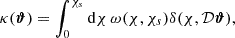 (1)
(1)
where χ is the comoving radial distance, χs is the radial distance to the source, and fK(χ) is the comoving angular distance,
 (2)
(2)
with K the spatial curvature. The lensing kernel ω(χ, χs) is defined as
 (3)
(3)
where c is the speed of light, Ωm is the matter density parameter, and H0 is the Hubble constant at z = 0.
The observed shear field γ(θ) relates to the convergence κ via mass inversion (Kaiser & Squires 1993; Starck et al. 2006; Martinet et al. 2015).
2.2. Angular Cls
Second-order statistics, such as the shear two-point correlation functions ξ±(θ) and their Fourier-space counterpart, the angular power spectrum Cℓ, play a crucial role in extracting cosmological information from weak-lensing surveys. These statistics describe the spatial distribution of the shear field and provide a window into the underlying matter distribution and its evolution.
Within the framework of the Limber approximation, the angular power spectrum of the convergence field for a specific tomographic bin is expressed as (Kilbinger 2015)
 (4)
(4)
where Pδ represents the matter power spectrum of the density contrast, χ denotes the comoving distance, and g(χ) is the lensing kernel that quantifies the lensing efficiency as a function of distance. The term a(χ) refers to the scale factor at a distance χ, while fK(χ) is the comoving angular diameter distance, determined by the spatial curvature of the Universe. This formulation enables us to compute the convergence power spectrum, which provides insights into structure growth and the geometry of the Universe by linking weak-lensing observables to the underlying matter distribution.
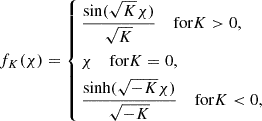
2.3. Shifted log-normal model
In cosmology, random fields such as the matter density contrast or lensing convergence are also described statistically using probability density functions (PDFs), which define how likely different values of the field are. For some fields, the PDF is well approximated by a Gaussian distribution.
Many cosmological fields deviate significantly from this Gaussian behaviour, however. For instance, the matter density contrast and lensing convergence have hard lower limits (e.g. density cannot drop below zero relative to the average) and exhibit skewed shapes with heavy tails, indicating a higher likelihood of extreme values compared to a Gaussian distribution. In these cases, a shifted log-normal (Coles & Jones 1991; Xavier et al. 2016; Tessore et al. 2023) distribution offers a better model and has emerged as a practical alternative to full N-body simulations. This distribution can account for the asymmetry, hard limits, and heavy tails observed in the data, providing a more realistic representation of the statistical behaviour of these fields.
This approach is particularly effective in capturing the non-Gaussian distribution of matter while accounting for the negative convergence values observed in specific scenarios. By shifting the log-normal distribution, the model extends its range to include regions with negative convergence, thereby improving the realism and accuracy of density fluctuation simulations. This enhancement is particularly valuable for representing under-dense regions while preserving the non-linear clustering effects of large-scale structures.
Under moderate noise levels and typical accuracy requirements, the log-normal model provides reliable covariance matrices and bispectra (Hall & Taylor 2022). The skewness of the log-normal model alone is insufficient to fully capture the nonlinear features induced by gravitational evolution, however, leading to inaccuracies in higher-order statistics (Piras et al. 2023).
Given a set of variables Kgi following a multivariate Gaussian distribution with mean vector μi and covariance matrix  , the shifted log-normal transformation is expressed as
 (5)
(5)
where λi depends on the cosmology and is computed as a function of the expected mean, variance, and skewness of the distribution. This dependence makes the model more flexible than a simple Gaussian approximation. Several approaches are used to fine-tune the shift parameter that is used in a log-normal model. The common approach is to focus on one scale of interest, and obtain a shift parameter such that the log-normal model has the correct skewness as that of the simulation, that is, it is calibrated against the PDF of the field at this particular scale, and that the shift parameter depends on the cosmology and on the scale. This means that fixing the shift parameter at one scale does not guarantee the exact skewness across all the other scales. Since convergence is not strictly a log-normal variable, different methods for determining λi yield different values, which might compromise the model accuracy at other scales. An added complexity arises when the matter density field is modelled as a log-normal field and integrated along the line of sight to derive the convergence map, which further complicates the estimation of λi. For further details, we refer to Xavier et al. (2016).
This log-normal transformation modifies the correlation function as follows (Xavier et al. 2016):
 (6)
(6)
Hence, to generate a log-normal field with the desired correlation function, the Gaussian field to which the local transformation is applied must first be constructed with a corrected correlation function. As expected, Equation (6) shows that the correlation function (and hence, the variance) is independent of the shift parameter, which is often calibrated so as to reproduce the expected skewness of the log-normal field. The correlation function is related to the power spectrum via
 (7)
(7)
where Pℓ represents the Legendre polynomial of order ℓ.
To illustrate the limitations inherent to the (shifted) log-normal model, we compared the convergence map generated using a log-normal model to a map derived from an N-body simulation. For this comparison, we used the publicly available Takahashi simulation suite (Takahashi et al. 2015), which provides full-sky convergence maps at a fixed cosmology1. These maps are available at two grid resolutions of 4096 and 8192, and they include data spanning the full sky at intervals of 150 h−1 comoving radial distance, covering redshifts from z = 0.05 to 5.3. The smoothing of the convergence maps is performed through a direct convolution of the map with a wavelet filter at specified angular scales. For this analysis, we used the convergence map at nside = 4096, which was subsequently downgraded to nside = 1024. A corresponding log-normal map with nside = 1024 and a maximum ℓ-mode of ℓmax = 3 nside + 1 was then generated for comparison. Figure 1 compares the distribution of a log-normally generated convergence map with N-body simulations. The shift parameter was optimised to match the distribution of the N-body simulation at a smoothing scale of θ = 20 arcmin. The figure illustrates that this configuration fails to hold at other scales or for the full map, however.
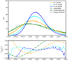 |
Fig. 1. Comparison of the one-point PDF from N-body simulations and from maps generated by shifted log-normal modelling. Top panel: Distributions of the shifted log-normally generated maps (solid lines) and N-body simulations (dashed lines) for the unsmoothed case (in green) and at a smoothing angle of θ = 5 arcmin, θ = 12 arcmin, and at θ = 20 arcmin, as labelled. Bottom panel: Relative residuals of the log-normal PDF with respect to the N-body simulation. |
This limitation underscores the necessity of developing a more flexible emulator capable of functioning consistently across all scales while effectively capturing cross-scale correlations. These advancements are crucial for robust multiscale analyses because they enable the extraction of non-linear information that is essential for cosmological inference.
3. Emulator based on the wavelet l1-norm theoretical prediction
Recent advancements in theoretical modelling have focused on higher-order statistics, such as the probability distribution function (PDF) (Barthelemy et al. 2021; Boyle et al. 2021) and the wavelet ℓ1-norm (Sreekanth et al. 2024), which are based on large deviation theory (LDT). These models have demonstrated the capability to provide accurate predictions of the one-point statistics (PDF and wavelet ℓ1-norm) of the density and convergence field up to mildly non-linear scales It was shown that for the wavelet ℓ1-norm of the convergence maps, a prediction can be obtained at subpercent accuracy for a κ map smoothed up to θ = 15 arcmin for a source redshift zs ≈ 2.
Our goal therefore was to build an emulator based on the theoretical prediction of the ℓ1-norm. In the following section, we describe our algorithm in detail, which we call Generative mOdeLling of Convergence maps based ON predicteD one-point stAtistics (GOLCONDA), and we present our results.
3.1. Wavelet ℓ1-norm
The wavelet transform is a powerful tool in the analysis of astronomical images because it can decompose data into components at different scales. This multi-scale decomposition is particularly effective for studying the complex hierarchical structures often found in astronomical data. We refer to Starck et al. (2015) for more details.
We employed a wavelet transform derived from using a tophat filter as the scaling function, as explained in (Sreekanth et al. 2024). An image c0 can then be decomposed as the sum of all wavelet scales and a coarse resolution image cJ,
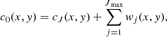 (8)
(8)
where Jmax denotes the maximum number of scales, and wj represents wavelet images that capture the details of the original image at dyadic scales j. Each set of wavelet coefficients wj was generated by convolving the input map with the respective wavelet kernel.
The wavelet ℓ1-norm is then defined as
![Mathematical equation: $$ \begin{aligned} \ell _1^{\theta _j}[i] = \sum _{k=1}^{\# coef(S_{\theta _j,i})} |S_{\theta _j,i}[k]|, \end{aligned} $$](/articles/aa/full_html/2025/09/aa54142-25/aa54142-25-eq10.gif) (9)
(9)
where the set of coefficients at scale θj and amplitude bin i, Sθj, i = {wθj / wθj(x,y)∈[Bi,Bi + 1]}, depicts the wavelet coefficients wθj having an amplitude within the bin [Bi, Bi + 1], and the pixel indices are given by (x, y). In other words, for each bin, the number of pixels k that fall in the bin waws collected, and the absolute values of these pixels were summed to obtain the ℓ1-norm at this bin i.
This definition allowed us to capture data through the absolute values of all pixels within the map instead of limiting the analysis to identifying local minima or maxima. It offers the benefit of a multi-scale approach and was shown to be particularly robust compared to other approaches (Huber 1987; Giné et al. 2003).
3.2. Theoretical prediction of the wavelet ℓ1-norm
Sreekanth et al. (2024) developed a theoretical framework to predict the wavelet ℓ1-norm, denoted as ℓ1θj[i], for weak-lensing convergence maps. This framework leverages LDT, which is a statistical method for describing rare events, to derive the one-point probability density function (PDF) of the convergence field. In this framework, the wavelet ℓ1-norm for a specific bin i is expressed as
![Mathematical equation: $$ \begin{aligned} \ell _1^{\theta _j}[i] = |S_{\theta _j,i}| \, P(S_{\theta _j,i}) \, \mathcal{N} , \end{aligned} $$](/articles/aa/full_html/2025/09/aa54142-25/aa54142-25-eq11.gif) (10)
(10)
where |Sθj, i| is the bin value (absolute value of the wavelet coefficient), P(Sθj, i) is the normalised PDF of the wavelet coefficients at scale θj, and 𝒩 is a factor accounting for the normalisation of the predicted PDF.
The theoretical predictions for ℓ1θj[i] were validated against results from N-body simulations and demonstrated agreement at the percent level. This approach provides an efficient and accurate alternative to computationally expensive simulations for analysing non-Gaussian features in weak-lensing data. For further details, we refer to Sreekanth et al. (2024).
Given the simplicity of predicting the wavelet ℓ1-norm for any specified cosmology, the objective was to use this prediction alongside the power spectrum as a constraint to generate a weak-lensing κ-map. The following section explores how these inputs can be effectively employed to produce a map that satisfies the desired statistical properties.
3.3. Optimisation problem
Our goal was to emulate a map with the statistical properties predicted by theoretical cosmological models for a given set of parameters. As the GLASS emulator, we wished to emulate a map κ that had the right theoretical power spectrum Pt, that is, 𝒫(κ) = Pt, where 𝒫 is the operator computing the radial power spectrum of κ. We also wished the same map to have the right distribution in the wavelet space as predicted by LDT. Noting, Wκ = {w1,…,wJ − 1,cJ − 1} the wavelet transform of κ using J scales, that is, W = Φtκ, and  the theoretical prediction in the different scales, each wavelet scale wj should have the correct l1-norm distribution ℓ1θj, i, that is, ℒ1θj(wj) = L1, tθj, where ℒ1θj is the operator calculating the ℓ1-norm at scale j following Eq. (9).
Specifically, we aimed to ensure that
-
The map had the correct theoretical power spectrum Pt,
 (11)
(11)where 𝒫 is the operator computing the radial power spectrum;
-
The wavelet coefficients of the map had the correct ℓ1-norm distribution at each scale,
 (12)
(12)where Wκ = {w1, …, wJ − 1, cJ − 1}=Φtκ is the wavelet transform, and ℒ1θj is the operator computing the ℓ1-norm at scale j.
We introduced two projection operators associated with these constraints:
-
𝒞f: The projection onto the space of maps satisfying the power spectrum constraint (Eq. (11)).
-
𝒞w: The projection onto the space of wavelet coefficients satisfying the ℓ1-norm constraints (Eq. (12)).
The problem is then formulated as a constrained optimisation,
 (13)
(13)
This minimisation ensures that κ and W are consistent throughout the wavelet transform while satisfying the power spectrum and wavelet norm constraints. Because these constraints correspond to different domains (Fourier and wavelet space), a joint solution is not trivial and requires an iterative strategy. The algorithm called generalised forward-backward (GFB) (Liang et al. 2015) is well suited for problems involving multiple non-smooth convex constraints. It enabled us to decompose the optimisation into simpler sub-problems associated with each constraint and to alternate between them efficiently while ensuring convergence. In our case, the algorithm alternated between applying the projections 𝒞f and 𝒞w while enforcing consistency between κ and W.
An alternative minimisation approach works as follows:
-
Assuming W is known, we minimise
 (14)
(14) -
Assuming κ is known, we minimise
 (15)
(15)
The GFB algorithm applied to this setup yields the following iterative update scheme:
-
-

-
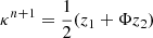
-
 .
.
Any additional summary statistics with theoretical prediction may be incorporated in a straightforward way by adding an additional constraint on κ.
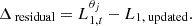
The  operator consists of i) taking the Fourier transform
  of κ, ii) computing its radial power spectrum Pκ, iii) multiplying the Fourier coefficients of
  by
by ![Mathematical equation: $ \sqrt{\frac{P_t [k] }{P_{\kappa} [k] }} $](/articles/aa/full_html/2025/09/aa54142-25/aa54142-25-eq25.gif) (i.e.
(i.e. ![Mathematical equation: $ z [u,v] = \sqrt{\frac{P_t [k] }{P_{\kappa} [k] }} \hat{\kappa} [u,v] $](/articles/aa/full_html/2025/09/aa54142-25/aa54142-25-eq26.gif) , with
, with  ), and iv) taking the inverse Fourier transform of z. Similarly, the
  operator independently adjusts the ℓ1-norm of all wavelet scales. The projection operators 𝒞f and 𝒞w are described in detail in Appendix A.
When Φ is orthogonal, we have ΦtΦ = Id, and step 2 of the previous equation becomes
 (16)
(16)
The method therefore becomes extremely simple by just iteratively applying the two steps
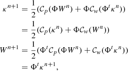 (17)
(17)
and we fixed κ0 to a Gaussian or log-normal realisation, and W0 = Φtκ0. In the most general cases, the wavelet transform is a frame and is not necessarily orthogonal. We therefore have ΦΦt = Id (because we have a transform with an exact reconstruction), but we do not always have ΦtΦ = Id. It remains a reasonable approximation, however, that allowed us to speed up the processing.
3.4. Algorithm
The algorithm iteratively adjusts an image to satisfy two main constraints: matching a target power spectrum through Fourier amplitude correction, and achieving desired ℓ1-norm wavelet coefficients. This iterative process ensures that the final image accurately represents both the specified statistical properties and the target power spectrum.
To do this, the algorithm begins with an initial image, a realisation of a 2D Gaussian random field in our case. It proceeds by iteratively refining the image through a two-step process. First, an ℓ1-norm-based wavelet coefficient adjustment (WCA) is applied to align the image wavelet coefficients with the desired properties. Second, the Fourier amplitudes are corrected to ensure that the image matches a specified target power spectrum. After each iteration, the refined image is obtained as a weighted average of the two corrected images. This iterative process continues until a convergence criterion, typically based on the relative root mean square (RMS) error between iterations, is satisfied or a predefined maximum number of iterations is reached. The algorithm involved here is given in Algorithm 1.
Input:
Initial map κ0
Maximum iterations max_iter
Tolerance ϵ
Output: Final map κ
1: Initialise κ ← κ0
2: Compute initial wavelet coefficients: W0 ← Φtκ0
3: forn = 1 to max_iterdo
4: Apply power spectrum constraint: z1 ← 𝒞p(ΦWn)
5: Apply wavelet ℓ1-norm constraint: z2 ← 𝒞w(Wn + Φt(κn − ΦWn))
6: Update the map: 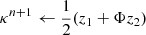
7: Update wavelet coefficients: 
8: Compute error: error ← RelativeRMS(κn + 1, κn)
9: iferror < ϵthen
10: Converged. Exit loop.
11: BREAK
12: end if
13: Update κ ← κn + 1
14: end for
15: returnκ
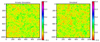 |
Fig. 2. Target convergence map and emulated convergence map obtained from our pipeline. The target map was obtained for a source redshift at zs = 2.134. The target and the generated maps both have a resolution of 1024 pixels on each side, with an angular size of 102 deg. The x- and y-axes give the number of pixels, and the pixel value is given by the color bar. |
4. Results and validation of the emulator
4.1. Simulations
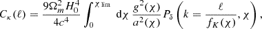
To test our pipeline, we used the suite called scinet light-cone simulations (SLICS) (Harnois-Déraps et al. 2018) of 924 fully independent N-body simulations that is publicly available2. They were derived from a set of 1025 N-body simulations generated using the high-performance gravity solver CUBEP3M (Harnois-Déraps et al. 2013), which computed the nonlinear evolution of 15363 particles starting from the initial conditions created at z = 120 using the Zeldovich approximation, in a box with a length of 505 h−1Mpc on one side. The N-body code calculated the non-linear evolution of these collisionless particles up to z = 0. Using a multiple-plane technique, we generated convergence and shear maps over an area of 100 square degrees at 18 distinct source planes using the Born approximation.
4.2. Validation
To evaluate the performance of our emulator, we conducted a series of tests using a target image that was wavelet-decomposed into multiple scales employing a tophat filter as the scaling function. The set of equations governing the wavelet decomposition was previously defined in equation (8). As mentioned previously, our approach was motivated by recent theoretical advancements using the wavelet ℓ1-norm, as predicted within the LDT framework (Sreekanth et al. 2024). These predictions provide input for generating emulated maps and are primarily valid in mildly non-linear scales, which consequently constrain the resolution of the maps. To demonstrate the effectiveness of this method, we validated our algorithm against the SLICS simulation suite.
We used a target image and decomposed it into a maximum of 2log(N) scales, where N is the number of pixels along one dimension of the map. This decomposition yielded 2log(N) sets of wavelet coefficients, along with a single coarse-scale image. The ℓ1-norm values, computed per bin for both the wavelet coefficients and the coarse-scale image, were treated as the target wavelet distributions. Simultaneously, the Cℓ values derived from the target image were designated as the target power spectra. Using these target distributions and power spectra as constraints, we applied the algorithm to generate emulated maps, which enabled us to assess its accuracy and robustness. For the validation, we generated a flat-sky map with a size of 100 deg2 with 1024 pixels on each side.
Figure 2 illustrates the original target image compared to the emulated image generated through our pipeline. The target image was derived from the N-body simulation, while our software produced the reconstructed solution. At first glance, no significant visual differences are observed between the target and the reconstructed images up to the phases that are different in the two cases.
During the iterative process, the relative error in the wavelet ℓ1-norms across different scales was assessed to evaluate the emulator performance. This error was calculated by comparing the ℓ1-norm of the wavelet coefficients and the coarse-scale coefficient of the reconstructed image to those of the target image. Convergence was determined based on the stabilisation of these relative errors, indicating that the emulator had successfully approximated the target distributions.
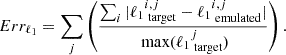
The number of iterations in this work was fixed at niter = 150, as multiple tests indicated good convergence at this value. This conclusion was reached after verifying that the overall relative error, defined in Equation (18), in the ℓ1-norm fell below 1%. This served as the convergence criterion to ensure that our iterative algorithm converged successfully. In our implementation, we set the tolerance Errℓ1 = 0.01, corresponding to a 1% relative error threshold. This value was chosen empirically, as we observed that both the ℓ1-norm and the power spectrum residuals reliably stabilised below this level, indicating convergence of the key statistical properties. While tighter thresholds are possible, we found that Errℓ1 = 0.01 offered a practical trade-off between computational cost and statistical accuracy. The convergence behaviour is shown in Figure 3, where the relative error falls below 1% within approximately 100 iterations. Equation (18) computes the total normalised absolute error between the target and emulated wavelet ℓ1-norms. For each scale j, it sums the absolute bin-wise differences over i, normalised by the maximum target value at that scale, and then sums over all scales.
 (18)
(18)
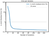 |
Fig. 3. Evolution of the total relative error (in %) in the ℓ1-norm of the reconstructed emulated image compared to the simulation map during the iterative process. The total relative error proves a measure of how closely the reconstructed image approximates the target simulation map. The stabilisation of this error indicates the convergence of the emulator with the target distribution. |
Figure 3 illustrates the evolution of the relative error over successive iterations. The plot highlights the error in the total ℓ1-norm of the emulated image compared to the target image. This result demonstrates the convergence of the algorithm and its capability to replicate the target distributions at different scales with high accuracy. The plot shows that the algorithm converges quickly and reaches an accuracy at the percent level at around 100 iterations.
To conduct a more comprehensive comparison, we analysed the statistical properties of the reconstructed map, focusing on the power spectrum and the wavelet ℓ1-norm. These comparisons are presented in Figures 4 and 5. Figure 4 presents the power spectra of the target κ map and the emulated map produced by our algorithm. The target power spectrum was derived from an N-body simulation, while the emulated power spectrum was generated using our pipeline, constrained by the input power spectrum and the wavelet ℓ1-norm. The figure also shows the residuals of the power spectra, calculated as the relative difference between the target and emulated spectra across all angular multipoles. These residuals consistently remained at a sub-percent level, demonstrating that the algorithm can replicate the target power spectrum with high precision.
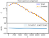 |
Fig. 4. Power spectra (Cℓ) of the target κ (solid orange line) map and the final emulated image (solid blue line) produced by our algorithm. The residuals (dashed green line) between the target and the emulated power spectra are also shown, indicating the level of agreement between the two maps. |
 |
Fig. 5. Wavelet ℓ1-norm at each scale and its residual between the decomposed target image (solid blue line) and the emulated image (dashed orange line) across different scales. The residuals, which are obtained as the difference between the target and the emulated wavelet ℓ1-norms, are also presented (dashed green line), reflecting the accuracy of the emulation process in reproducing the target distributions. |
In Figure 5, we present the wavelet ℓ1-norm of the decomposed image at various scales. The comparison highlights the wavelet ℓ1-norm values computed for the target wavelet coefficients and those obtained from the emulated wavelet coefficients at each scale. The residuals, shown alongside, quantify the differences between the target and emulated wavelet ℓ1-norms. Across all scales, the residuals are also at a sub-percent level, confirming the accuracy of the emulator in reproducing the target wavelet distributions.
These results emphasise the robustness of our algorithm, which successfully captures both the global and scale-dependent statistical properties of the target map. The sub-percent residuals observed in both the power spectrum and wavelet ℓ1-norm validate the consistency of our approach and its potential for applications in cosmological analyses where precision is critical.
4.3. Benchmarking
In this section, we explore the time complexity, statistical properties, and higher-order statistics of the generated maps at multiple scales using different wavelet and smoothing filters (i.e. beyond the constraints used by the algorithm). This analysis provides insights into the strengths and limitations of the algorithm, highlighting its ability to emulate realistic data with minimum computational resources.
4.3.1. Performance
To generate the plots, our pipeline was able to generate each 500 × 500 map in less than 2 min. The Figure 6 below presents a plot of the processing time against map size. We used a single CPU and one core without incorporating any parallelisation or just-in-time (JIT) compilation, but it still performed comparably or better than existing methods.
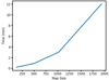 |
Fig. 6. Time complexity of the generator. The x-axis shows the number of pixels on each side. On the y-axis, we plot the time taken to generate a map for the given size. |
4.3.2. Higher cumulants
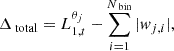
We further examined the statistical properties embedded in the maps, including skewness, variance, and kurtosis, at various scales over the entire map. To estimate the associated error bars, we divided each map into four patches and computed the standard deviation of the moments obtained across these patches. These results are displayed in Figure 7. The analysis was performed by dividing both the target and reconstructed maps into sub-patches, which allowed us to compute these statistics across the entire map and to estimate the associated uncertainties.
 |
Fig. 7. Variance and skewness for the target image (in red) and the emulated image (in blue) obtained using a tophat scaling function to derive the wavelet. The emulated image was created by an algorithm that matched the wavelet ℓ1-norm of the target image from the SLICS simulation. Benchmarking was conducted by smoothing both images with different radii via a tophat filter, partitioning them into patches, and calculating skewness, variance, kurtosis, and their associated error bars by taking the standard deviation of the values obtained from four different patches of the maps. The x-axis represents the smoothing scale in arcminutes. |
The left panel shows the skewness, which quantifies the asymmetry of the distribution of pixel values in the maps. The skewness values and associated errors of the target (red) and reconstructed (blue) maps agree closely, demonstrating the ability of the reconstruction process to preserve the asymmetry of the target map.
The middle panel presents the variance, which measures the dispersion of pixel values. As expected, the variance decreases with increasing smoothing scale due to the suppression of small-scale fluctuations during smoothing. The reconstructed map successfully reproduces the variance in the target map at all scales, with a good overlap between the red and blue points within the error bars.
The right panel shows the kurtosis, which captures the degree of tailedness in the distribution of the pixel values. The kurtosis generally decreases with increasing smoothing scale, consistent with the suppression of higher-order moments in smoothed data. The reconstructed map closely matches the kurtosis of the target map, with only minor deviations at some scales.
The results indicate that the reconstruction process preserves the higher-order statistical properties of the target map overall, as evidenced by the close agreement across skewness, variance, and kurtosis.
Appendix B presents some additional tests that omitted other higher-order statistics, namely PDFs and peak counts, showing that they incidentally match very well (within the statistical errors of the numerical experiment).
4.4. Extension to the generation of full-sky maps
Extending the algorithm to full-sky maps is a straightforward process because the method remains applicable in this setting. To do this, we used (Zonca et al. 2019; Górski et al. 2005). This extension has already been implemented, and the corresponding full-sky version is publicly available. Further details, including access to the implementation, can be found in Section ‘Data availability’.
5. Generalisation of the emulator to theoretical constraints
The validation presented in this work relies on a target wavelet ℓ1-norm extracted from a simulation-generated weak- lensing convergence map. The method developed here is not restricted to this specific validation case, however. In principle, the emulator allows us to substitute the target values with any external input, including an arbitrary combination of a theoretical power spectrum Cℓ and a corresponding set of ℓ1-norm values across wavelet scales. This adaptability enables the generation of statistically controlled convergence maps, making it possible to impose user-defined constraints without an explicit dependence on simulation-based training data, which could come from purely theoretical grounds.
A notable advantage of this flexibility is the ability to incorporate stochasticity directly at the level of the input statistics so as to account for cosmic variance. In particular, any desired level of variance or non-Gaussian features arising from cosmic structure formation can be included by explicitly modulating the input target values. This approach allows us to control the sampling of cosmic variance, either by introducing uncertainty in the power spectrum Cℓ or by perturbing the predicted ℓ1-norms within physically motivated bounds. Consequently, the emulator can be extended to produce ensembles of statistically consistent weak-lensing maps that account for inherent fluctuations, thereby offering an alternative to expensive numerical simulations. One approach to achieve this might be to incorporate the cosmic variance at the level of the power spectrum only (see e.g. Moster et al. 2011) and obtain the corresponding wavelet ℓ1-norm by only changing the power spectrum and keeping the scaled cumulants fixed Codis et al. (2016).
A fundamental limitation of using the theoretical prediction to generate maps is its dependence on scale. The derivation constrains the statistical properties of the wavelet ℓ1-norm only up to mildly non-linear scales, as we discussed before. For scales smaller than the constrained range, however, the generated map may not accurately reproduce the statistical properties of the simulation.
Figure 8 shows an example of a map obtained by applying the constraints from the theory predictions at the first three scales (which includes the three wavelet coefficients and one coarse-scale coefficient). We also compared the wavelet ℓ1-norm of the generated map with the theoretical predictions at the constrained scales, as shown in Figure 9. The figure clearly shows that the generated map successfully reproduces the theoretical ℓ1-norm values with high accuracy. The residuals consistently remain at a sub-percent level, demonstrating the precision of the reconstruction and the effectiveness of the algorithm. The small oscillations in the residuals are attributed to the finite patch size used in the analysis.
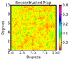 |
Fig. 8. Emulated convergence map produced by our pipeline with a pixel size of 2 arcmin, generated by applying constraints on the first three scales for which the theory-based wavelet ℓ1-norm is obtained. The x- and y-axes represent the map range in degrees, and the pixel values are indicated by the colour bar. |
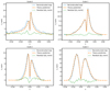 |
Fig. 9. Comparison of the wavelet ℓ1-norm of the generated map (solid blue line) with the theoretical predictions (dashed orange line) across different scales ranging from 2 to 8 arcmin, shown from the top left to the bottom right panel. The final panel represents the coarse scale at 8 arcmin. The residuals (solid green line) between the target and emulated wavelet ℓ1-norms are also shown, indicating the accuracy of the emulation process in reproducing the expected distributions. |
6. Conclusions
We developed and benchmarked a novel map-emulation algorithm that uses wavelet-based approaches, such as the tophat filter, to generate high-fidelity convergence maps with an enhanced accuracy and computational efficiency. Our method can emulate maps of 500 pixels per side in approximately one minute, even when it is restricted to a single CPU core and without parallelisation or just-in-time compilation. This performance underscores that our approach is more practical than traditional methods, which typically require substantial computational resources. The efficiency of the pipeline, coupled with its statistical rigour, provides a strong foundation for generating realistic cosmological maps in various applications.
A key focus of our work was the preservation and accurate reproduction of higher-order statistics, including variance, skewness, and kurtosis, at different scales and across entire maps. By conducting a thorough benchmarking analysis with a tophat filter, we demonstrated that our emulated maps closely approximate the statistical properties of target datasets, such as those derived from SLICS simulations. This capability to capture essential features of the underlying data makes our method particularly relevant for applications requiring precise modelling of small-scale structures and non-Gaussian features in cosmological fields.
Our results illustrate that the statistical alignment of the pipeline extends beyond basic moments, with a robust performance in reproducing higher-order metrics such as the cumulants across various smoothing scales apart from those used for constraining. This accuracy in representing complex structures suggests that our method provides a meaningful alternative to existing techniques, particularly log-normal map generation, which may not fully encapsulate higher-order dependencies and non-linear structures found in observed data.
Furthermore, the adaptability of our method offers promising opportunities for extensions and practical applications. The flexibility of the emulator enables the substitution of target values with any external input, including theoretical power spectra Cℓ and corresponding sets of ℓ1-norm values across wavelet scales. This adaptability allowed us to generate statistically controlled convergence maps with user-defined constraints without an explicit reliance on simulation-based training data. Additionally, the ability to incorporate stochasticity at the input level provides a means to model cosmic variance explicitly. This extends the ability of the emulator to produce ensembles of statistically consistent weak-lensing maps that account for inherent fluctuations.
While the current implementation of our algorithm is designed to reproduce specific one- and two-point statistics (namely, the wavelet ℓ1-norm and the power spectrum) under idealised conditions, its modular structure allows a considerable flexibility. In particular, the framework can naturally be extended to incorporate observational systematics and physical effects. For instance, if theoretical predictions or simulation-based estimates of the wavelet ℓ1-norm and power spectrum are available for convergence fields affected by intrinsic alignments or baryonic feedback, these can be directly used as constraints in the emulator. This enables the generation of convergence maps that encode the impact of these effects without requiring explicit modelling of the underlying processes. Moreover, although systematics such as shear calibration errors and photometric redshift uncertainties typically arise earlier in the weak-lensing analysis pipeline, the algorithm outputs can serve as inputs to downstream inference frameworks that incorporate these sources of uncertainty. Alternatively, the generated maps can be post-processed to simulate survey-specific features, including shape noise, masking, and selection biases. In summary, while this work has focused on validating the method in idealised scenarios, the design of the algorithm lends itself to future extensions that incorporate realistic systematics and survey conditions either through modified input constraints or post-processing.
Given these demonstrated capabilities, our wavelet-based emulation approach emerges as a robust and computationally efficient tool that might replace or complement log-normal map-generation techniques. By accurately preserving both higher-order statistics and fine-scale structures, our method offers a more complete representation of complex cosmological fields. Future developments may focus on optimising the algorithm through parallelisation and JIT techniques, expanding its usability and applicability across a wider range of datasets and scales. Furthermore, this method has potential applications in inpainting. Inpainting techniques aim to reconstruct missing data in an image or signal by estimating the absent values from the available information. Various approaches, such as sparse inpainting using the discrete cosine transform (Starck et al. 2005a,b), sparse recovery techniques (Pires et al. 2009; Lanusse et al. 2016), and Gaussian-constrained realisations (Zaroubi et al. 1995; Jeffrey et al. 2018), have been widely explored in the literature. The algorithm we presented might also prove useful for inpainting. While this exploration lies beyond the scope of this paper, assessing the effectiveness of this method compared to existing inpainting techniques remains an intriguing avenue for future research.
In conclusion, this work sets a foundation for efficient, accurate, and adaptable map-emulation strategies, offering significant potential for advancing cosmological data analysis, large-scale simulations, and other applications where statistical fidelity and computational efficiency are paramount.
Data availability
The code GOLCONDA (Generative mOd-eLing of Convergence maps based ON predicteD one-point stAtistics) is made available in the spirit of open research. It enabled us to reproduce the plots and can be accessed at GitHub.
SLICS: https://slics.roe.ac.uk
Acknowledgments
This work was supported by the TITAN ERA Chair project (contract no. 101086741) within the Horizon Europe Framework Program of the European Commission, and the Agence Nationale de la Recherche (ANR-22-CE31-0014-01 TOSCA). We would like to thank Joachim Harnois-Déraps for making public the SLICS mock data, which can be found at http://slics.roe.ac.uk/. We would also like to thank Takahashi and collaborators for making public the TAKAHASHI simulation suite, which can be found at http://cosmo.phys.hirosaki-u.ac.jp/takahasi/allsky_raytracing/. The authors thank Andreas Tersenov, Cora Uhlemann and Alexandre Barthelemy for useful discussions.
References
- Ajani, V., Peel, A., Pettorino, V., et al. 2020, Phys. Rev. D, 102, 103531 [Google Scholar]
- Ajani, V., Starck, J.-L., & Pettorino, V. 2021, A&A, 645, L11 [NASA ADS] [CrossRef] [EDP Sciences] [Google Scholar]
- Alsing, J., Heavens, A., Jaffe, A. H., et al. 2016, MNRAS, 455, 4452 [Google Scholar]
- Alsing, J., Wandelt, B., & Feeney, S. 2018, MNRAS, 477, 2874 [NASA ADS] [CrossRef] [Google Scholar]
- Barthelemy, A., Codis, S., & Bernardeau, F. 2021, MNRAS, 503, 5204 [Google Scholar]
- Bernardeau, F., & Valageas, P. 2000, A&A, 364, 1 [NASA ADS] [Google Scholar]
- Böhm, V., Hilbert, S., Greiner, M., & Enßlin, T. A. 2017, Phys. Rev. D, 96, 123510 [CrossRef] [Google Scholar]
- Boruah, S. S., Fiedorowicz, P., Garcia, R., et al. 2024, arXiv e-prints [arXiv:2406.05867] [Google Scholar]
- Boyle, A., Uhlemann, C., Friedrich, O., et al. 2021, MNRAS, 505, 2886 [NASA ADS] [CrossRef] [Google Scholar]
- Cheng, S., & Ménard, B. 2021, MNRAS, 507, 1012 [NASA ADS] [CrossRef] [Google Scholar]
- Codis, S., Bernardeau, F., & Pichon, C. 2016, MNRAS, 460, 1598 [NASA ADS] [CrossRef] [Google Scholar]
- Coles, P., & Jones, B. 1991, MNRAS, 248, 1 [NASA ADS] [CrossRef] [Google Scholar]
- Dai, B., & Seljak, U. 2022, MNRAS, 516, 2363 [NASA ADS] [CrossRef] [Google Scholar]
- Dai, B., & Seljak, U. 2023, in Machine Learning for Astrophysics, 10 [Google Scholar]
- Fagioli, M., Tortorelli, L., Herbel, J., et al. 2020, JCAP, 2020, 050 [CrossRef] [Google Scholar]
- Feng, Y., Chu, M.-Y., Seljak, U., & McDonald, P. 2016, MNRAS, 463, 2273 [NASA ADS] [CrossRef] [Google Scholar]
- Fluri, J., Kacprzak, T., Refregier, A., et al. 2018, Phys. Rev. D, 98, 123518 [NASA ADS] [CrossRef] [Google Scholar]
- Fluri, J., Kacprzak, T., Lucchi, A., et al. 2019, Phys. Rev. D, 100, 063514 [Google Scholar]
- Gatti, M., Chang, C., Friedrich, O., et al. 2020, MNRAS, 498, 4060 [Google Scholar]
- Gatti, M., Campailla, G., Jeffrey, N., et al. 2024, arXiv e-prints [arXiv:2405.10881] [Google Scholar]
- Giné, E., Mason, D. M., & Zaitsev, A. Y. 2003, Ann. Probab., 31, 719 [Google Scholar]
- Górski, K. M., Hivon, E., Banday, A. J., et al. 2005, ApJ, 622, 759 [Google Scholar]
- Hall, A., & Taylor, A. 2022, Phys. Rev. D, 105, 123527 [NASA ADS] [CrossRef] [Google Scholar]
- Harnois-Déraps, J., Pen, U.-L., Iliev, I. T., et al. 2013, MNRAS, 436, 540 [Google Scholar]
- Harnois-Déraps, J., Amon, A., Choi, A., et al. 2018, MNRAS, 481, 1337 [Google Scholar]
- Heymans, C., Van Waerbeke, L., Miller, L., et al. 2012, MNRAS, 427, 146 [Google Scholar]
- Hilbert, S., Hartlap, J., & Schneider, P. 2011, A&A, 536, A85 [NASA ADS] [CrossRef] [EDP Sciences] [Google Scholar]
- Huber, P. J. 1987, Comput. Stat. Data Anal., 5, 255 [CrossRef] [Google Scholar]
- Huterer, D. 2010, Gen. Rel. Grav., 42, 2177 [Google Scholar]
- Ivezić, Ž., Kahn, S. M., Tyson, J. A., et al. 2019, ApJ, 873, 111 [Google Scholar]
- Izard, A., Crocce, M., & Fosalba, P. 2016, MNRAS, 459, 2327 [NASA ADS] [CrossRef] [Google Scholar]
- Jeffrey, N., Abdalla, F. B., Lahav, O., et al. 2018, MNRAS, 479, 2871 [Google Scholar]
- Jeffrey, N., Alsing, J., & Lanusse, F. 2021, MNRAS, 501, 954 [Google Scholar]
- Kaiser, N., & Squires, G. 1993, ApJ, 404, 441 [Google Scholar]
- Kilbinger, M. 2015, Rep. Prog. Phys., 78, 086901 [Google Scholar]
- Kitaura, F. S., Yepes, G., & Prada, F. 2014, MNRAS, 439, L21 [NASA ADS] [CrossRef] [Google Scholar]
- Kratochvil, J. M., Lim, E. A., Wang, S., et al. 2012, Phys. Rev. D, 85, 103513 [Google Scholar]
- Kruse, G., & Schneider, P. 1999, MNRAS, 302, 821 [Google Scholar]
- Lanusse, F., Starck, J.-L., Leonard, A., & Pires, S. 2016, A&A, 591, A2 [NASA ADS] [CrossRef] [EDP Sciences] [Google Scholar]
- Lanzieri, D., Lanusse, F., Modi, C., et al. 2023, A&A, 679, A61 [NASA ADS] [CrossRef] [EDP Sciences] [Google Scholar]
- Laureijs, R., Amiaux, J., Arduini, S., et al. 2011, arXiv e-prints [arXiv:1110.3193] [Google Scholar]
- Lesgourgues, J., & Pastor, S. 2012, Adv. High Energy Phys., 2012, 1 [CrossRef] [Google Scholar]
- Li, Z., Liu, J., Zorrilla Matilla, J. M., & Coulton, W. R. 2019, Phys. Rev. D, 99, 063527 [NASA ADS] [CrossRef] [Google Scholar]
- Liang, J., Fadili, J., & Peyré, G. 2015, arXiv e-prints [arXiv:1503.03703] [Google Scholar]
- Lin, C.-A., & Kilbinger, M. 2015, A&A, 583, A70 [NASA ADS] [CrossRef] [EDP Sciences] [Google Scholar]
- Liu, J., & Madhavacheril, M. S. 2019, Phys. Rev. D, 99, 083508 [Google Scholar]
- Liu, J., Petri, A., Haiman, Z., et al. 2015a, Phys. Rev. D, 91, 063507 [Google Scholar]
- Liu, X., Pan, C., Li, R., et al. 2015b, MNRAS, 450, 2888 [Google Scholar]
- Mandelbaum, R., & Hyper Suprime-Cam HSC Collaboration 2017, Am. Astron. Soc. Meeting Abstr., 229, 226 [Google Scholar]
- Martinet, N., Bartlett, J. G., Kiessling, A., & Sartoris, B. 2015, A&A, 581, A101 [NASA ADS] [CrossRef] [EDP Sciences] [Google Scholar]
- Mellier, Y. 1999, ARA&A, 37, 127 [NASA ADS] [CrossRef] [Google Scholar]
- Moster, B. P., Somerville, R. S., Newman, J. A., & Rix, H.-W. 2011, ApJ, 731, 113 [Google Scholar]
- Papamakarios, G., Murray, I., & Pavlakou, T. 2017, Advances in Neural Information Processing Systems 30, NIPS 2017 [Google Scholar]
- Parroni, C., Cardone, V. F., Maoli, R., & Scaramella, R. 2020, A&A, 633, A71 [NASA ADS] [CrossRef] [EDP Sciences] [Google Scholar]
- Peel, A., Lin, C.-A., Lanusse, F., et al. 2017, A&A, 599, A79 [NASA ADS] [CrossRef] [EDP Sciences] [Google Scholar]
- Peel, A., Pettorino, V., Giocoli, C., Starck, J.-L., & Baldi, M. 2018, A&A, 619, A38 [NASA ADS] [CrossRef] [EDP Sciences] [Google Scholar]
- Petri, A. 2016, Astron. Comput., 17, 73 [NASA ADS] [CrossRef] [Google Scholar]
- Piras, D., Joachimi, B., & Villaescusa-Navarro, F. 2023, MNRAS, 520, 668 [Google Scholar]
- Pires, S., Starck, J. L., Amara, A., et al. 2009, MNRAS, 395, 1265 [Google Scholar]
- Porqueres, N., Heavens, A., Mortlock, D., Lavaux, G., & Makinen, T. L. 2023, arXiv e-prints [arXiv:2304.04785] [Google Scholar]
- Remy, B., Lanusse, F., Jeffrey, N., et al. 2023, A&A, 672, A51 [NASA ADS] [CrossRef] [EDP Sciences] [Google Scholar]
- Ribli, D., Pataki, B. A., Zorrilla Matilla, J. M., et al. 2019, MNRAS, 490, 1843 [CrossRef] [Google Scholar]
- Rodríguez, A. C., Kacprzak, T., Lucchi, A., et al. 2018, Comput. Astrophys. Cosmol., 5, 4 [Google Scholar]
- Scoccimarro, R., & Sheth, R. K. 2002, MNRAS, 329, 629 [NASA ADS] [CrossRef] [Google Scholar]
- Sharma, D., Dai, B., & Seljak, U. 2024, JCAP, 08, 010 [Google Scholar]
- Sreekanth, V. T., Codis, S., Barthelemy, A., & Starck, J.-L. 2024, A&A, 691, A80 [NASA ADS] [CrossRef] [EDP Sciences] [Google Scholar]
- Starck, J.-L., Elad, M., & Donoho, D. 2005a, IEEE Trans. Image Process., 14, 1570 [Google Scholar]
- Starck, J.-L., Moudden, Y., Bobin, J., & Elad, M. 2005b, in Wavelets XI (SPIE), 5914, 209 [Google Scholar]
- Starck, J. L., Pires, S., & Réfrégier, A. 2006, A&A, 451, 1139 [NASA ADS] [CrossRef] [EDP Sciences] [Google Scholar]
- Starck, J.-L., Murtagh, F., & Fadili, J. 2015, Sparse image and signal processing: Wavelets and related geometric multiscale analysis, second edition, (Cambridge University Press), 428 [Google Scholar]
- Takahashi, R., Hamana, T., Shirasaki, M., et al. 2017, ApJ, 850, 24 [Google Scholar]
- Tassev, S., Zaldarriaga, M., & Eisenstein, D. J. 2013, JCAP, 2013, 036 [Google Scholar]
- Tessore, N., Loureiro, A., Joachimi, B., von Wietersheim-Kramsta, M., & Jeffrey, N. 2023, Open J. Astrophys., 6, 11 [NASA ADS] [CrossRef] [Google Scholar]
- Tortorelli, L., Fagioli, M., Herbel, J., et al. 2020, JCAP, 2020, 048 [CrossRef] [Google Scholar]
- Troxel, M., & Ishak, M. 2015, Phys. Rep., 558, 1 [NASA ADS] [CrossRef] [Google Scholar]
- White, M., Tinker, J. L., & McBride, C. K. 2014, MNRAS, 437, 2594 [NASA ADS] [CrossRef] [Google Scholar]
- Xavier, H. S., Abdalla, F. B., & Joachimi, B. 2016, MNRAS, 459, 3693 [NASA ADS] [CrossRef] [Google Scholar]
- Yu, Y., Zhang, P., & Jing, Y. 2016, Phys. Rev. D, 94, 083520 [Google Scholar]
- Zaroubi, S., Hoffman, Y., Fisher, K. B., & Lahav, O. 1995, ApJ, 449, 446 [Google Scholar]
- Zonca, A., Singer, L., Lenz, D., et al. 2019, J. Open Source Software, 4, 1298 [Google Scholar]
Appendix A: Algorithm in detail
A.1. ℓ1-Norm matching wavelet coefficient adjustment algorithm
We are using the ℓ1-Norm Matching Wavelet Coefficient Adjustment Algorithm (ℓ1-WCA), which is designed to adjust wavelet coefficients at various scales to achieve specified ℓ1 norms within predefined histogram bins. This algorithm iteratively modifies the wavelet coefficients in each bin, separately adjusting positive and negative values to meet target ℓ1 norms while ensuring the values remain within set boundaries. We believe it could be useful in applications where specific statistical properties of wavelet-transformed data must be preserved, providing a flexible method to enforce norm constraints without disrupting the underlying data distribution.
Given a target L1, t, ℓ1 of the wavelet coefficient can be adjusted to match the target as follows:
First, the total adjustment Δtotal is obtained as the difference between the target and the current wavelet ℓ1-norm.
 (A.1)
(A.1)
where L1, tθj represents the target ℓ1-norm at scale j, and the summation computes the current ℓ1-norm of the wavelet coefficients. This is used to get the adjustment per positive coefficient as:
 (A.2)
(A.2)
where Np is the number of positive coefficients. The adjusted positive coefficients are then given by:
 (A.3)
(A.3)
After this update, the new ℓ1 is computed as:
 (A.4)
(A.4)
The remaining adjustment to the target norm is obtained as:
 (A.5)
(A.5)
The residual is distributed amongst the negative coefficients and updated as:
 (A.6)
(A.6)
This now gives a wavelet coefficient with the constrained ℓ1-norm matching the target.
The corresponding algorithm is given in Algorithm A.1.
A.2. Algorithm for getting the correct power spectra
To generate an image with the desired target power spectrum (Cls), we perform Fourier amplitude rescaling. This process adjusts the Fourier amplitudes of the image to match the target power spectrum while preserving the original phase information to maintain spatial structure, as shown in Algorithm 3.
Input:
Wavelet coefficient set at scale j: wj
Target ℓ1-norm: L1, tθj
Number of histogram bins: Nbin
Output: Adjusted wavelet coefficients wj
1: Compute current ℓ1-norm: 
2: Compute total adjustment: Δtotal = L1, tθj − L1, c
3: Compute adjustment per positive coefficient:  , where Np is the number of positive coefficients
4: for each coefficient wj, ido
5: ifwj, i ≥ 0 then
6: wj, i ← max(wj, i + Δp, 0)
7: end if
8: end for
9: Compute updated ℓ1-norm: 
10: Compute residual adjustment: Δresidual = L1, tθj − L1, updated
11: Compute adjustment per negative coefficient:  , where Nn is the number of negative coefficients
12: for each coefficient wj, ido
13: ifwj, i < 0 then
14: wj, i ← min(wj, i − Δn, 0)
15: end if
16: end for
17: for each coefficient wj, ido
18: Enforce boundaries: wj, i ← max(min(wj, i, BoundMax),BoundMin)
19:end for
20: returnwj
Input:
Input map κ
Target power spectrum Pt
Output: Adjusted map κ′
1: Compute the Fourier transform of the input map: ![Mathematical equation: $ \hat{\kappa}(\mathbf{k}) = \mathcal{F}[\kappa] $](/articles/aa/full_html/2025/09/aa54142-25/aa54142-25-eq44.gif)
2: Compute the radial power spectrum of the input map: 
3: Compute the rescaling factor: 
4: Rescale the Fourier amplitudes: 
5: Perform the inverse Fourier transform to obtain the adjusted map: ![Mathematical equation: $ \kappa{\prime}= \mathcal{F}^{-1}[\hat{\kappa}{\prime}(\mathbf{k})] $](/articles/aa/full_html/2025/09/aa54142-25/aa54142-25-eq48.gif)
6: returnκ′
Appendix B: Evaluation of higher-order statistics
We conducted a detailed comparison of the emulated convergence maps with the target maps, focusing on the one-point Probability Distribution Function (PDF) and peak counts. In addition to the main analysis presented in the main text, we have also conducted a detailed comparison of the emulated convergence maps with the target maps using other high-order statistics. We have especially focused on the one-point Probability Distribution Function (PDF) and peak counts, which are detailed below.
B.1. Probability distribution function (PDF)
Figure B.1 shows the one-point PDF of the convergence field at two different smoothing scales (2 arcmin and 12 arcmin), obtained using a circular tophat filter. These filters are distinct from the wavelet-like difference-of-top hats used in defining the ℓ1-norm constraint. The top panels show the PDFs for both the target and emulated maps, while the bottom panels display the residuals. The results indicate agreement at the ∼10% level across most of the distribution, with slight discrepancies in the extreme tails. Let us note that for intermediate to large smoothing scales (e.g. 12 arcmin here), the difference is entirely within the statistical error bars of our measurements, hence no significant departure is observed in this regime. For smaller smoothing scales, the deviation is more significant, but this is in a regime where non-linearities start to be quite important (hence less interesting for cosmological analysis if systematics can not be controlled), and resolution effects might also play a significant role.
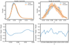 |
Fig. B.1. Top panels: One-point PDF of the target and emulated maps at two smoothing scales (2 and 12 arcmin), computed using a circular tophat filter. Bottom panels: Residuals between emulated and target PDFs. |
B.2. Peak count statistics
In Figure B.2, we show the peak count distribution at various wavelet scales. Peaks are defined as local maxima in the map, and the histograms are shown separately for the target and emulated maps. The agreement is very good for all scales, with some fluctuation at the largest scales (4 and 5), mostly driven by a lack of statistics.
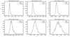 |
Fig. B.2. Peak count distribution at different wavelet scales as labelled for the target (dotted red line) and emulated maps (blue solid line). Emulated maps reproduce the peak counts of the target with high fidelity at small to intermediate scales. |
B.3. Implications for higher-order moments
Although the algorithm is optimised only to match the power spectrum and wavelet ℓ1-norm, the consistency seen in the PDFs and peak counts, especially in the tails, indicates that higher-order moments are approximately preserved. These statistics, especially the peak counts, are sensitive to non-Gaussian features and implicitly reflect the presence of higher-order correlations beyond the fourth moment. However, we emphasise that our method does not guarantee fidelity in any specific higher-order moment. The observed agreement suggests the approach generalises well and captures broader statistical features, but also leaves room for future improvements that target additional moments explicitly.
All Figures
|
Fig. 1. Comparison of the one-point PDF from N-body simulations and from maps generated by shifted log-normal modelling. Top panel: Distributions of the shifted log-normally generated maps (solid lines) and N-body simulations (dashed lines) for the unsmoothed case (in green) and at a smoothing angle of θ = 5 arcmin, θ = 12 arcmin, and at θ = 20 arcmin, as labelled. Bottom panel: Relative residuals of the log-normal PDF with respect to the N-body simulation. |
| In the text | |
|
Fig. 2. Target convergence map and emulated convergence map obtained from our pipeline. The target map was obtained for a source redshift at zs = 2.134. The target and the generated maps both have a resolution of 1024 pixels on each side, with an angular size of 102 deg. The x- and y-axes give the number of pixels, and the pixel value is given by the color bar. |
| In the text | |
|
Fig. 3. Evolution of the total relative error (in %) in the ℓ1-norm of the reconstructed emulated image compared to the simulation map during the iterative process. The total relative error proves a measure of how closely the reconstructed image approximates the target simulation map. The stabilisation of this error indicates the convergence of the emulator with the target distribution. |
| In the text | |
|
Fig. 4. Power spectra (Cℓ) of the target κ (solid orange line) map and the final emulated image (solid blue line) produced by our algorithm. The residuals (dashed green line) between the target and the emulated power spectra are also shown, indicating the level of agreement between the two maps. |
| In the text | |
|
Fig. 5. Wavelet ℓ1-norm at each scale and its residual between the decomposed target image (solid blue line) and the emulated image (dashed orange line) across different scales. The residuals, which are obtained as the difference between the target and the emulated wavelet ℓ1-norms, are also presented (dashed green line), reflecting the accuracy of the emulation process in reproducing the target distributions. |
| In the text | |
|
Fig. 6. Time complexity of the generator. The x-axis shows the number of pixels on each side. On the y-axis, we plot the time taken to generate a map for the given size. |
| In the text | |
|
Fig. 7. Variance and skewness for the target image (in red) and the emulated image (in blue) obtained using a tophat scaling function to derive the wavelet. The emulated image was created by an algorithm that matched the wavelet ℓ1-norm of the target image from the SLICS simulation. Benchmarking was conducted by smoothing both images with different radii via a tophat filter, partitioning them into patches, and calculating skewness, variance, kurtosis, and their associated error bars by taking the standard deviation of the values obtained from four different patches of the maps. The x-axis represents the smoothing scale in arcminutes. |
| In the text | |
|
Fig. 8. Emulated convergence map produced by our pipeline with a pixel size of 2 arcmin, generated by applying constraints on the first three scales for which the theory-based wavelet ℓ1-norm is obtained. The x- and y-axes represent the map range in degrees, and the pixel values are indicated by the colour bar. |
| In the text | |
|
Fig. 9. Comparison of the wavelet ℓ1-norm of the generated map (solid blue line) with the theoretical predictions (dashed orange line) across different scales ranging from 2 to 8 arcmin, shown from the top left to the bottom right panel. The final panel represents the coarse scale at 8 arcmin. The residuals (solid green line) between the target and emulated wavelet ℓ1-norms are also shown, indicating the accuracy of the emulation process in reproducing the expected distributions. |
| In the text | |
|
Fig. B.1. Top panels: One-point PDF of the target and emulated maps at two smoothing scales (2 and 12 arcmin), computed using a circular tophat filter. Bottom panels: Residuals between emulated and target PDFs. |
| In the text | |
|
Fig. B.2. Peak count distribution at different wavelet scales as labelled for the target (dotted red line) and emulated maps (blue solid line). Emulated maps reproduce the peak counts of the target with high fidelity at small to intermediate scales. |
| In the text | |
Current usage metrics show cumulative count of Article Views (full-text article views including HTML views, PDF and ePub downloads, according to the available data) and Abstracts Views on Vision4Press platform.
Data correspond to usage on the plateform after 2015. The current usage metrics is available 48-96 hours after online publication and is updated daily on week days.
Initial download of the metrics may take a while.