| Issue |
A&A
Volume 701, September 2025
|
|
|---|---|---|
| Article Number | A26 | |
| Number of page(s) | 12 | |
| Section | Extragalactic astronomy | |
| DOI | https://doi.org/10.1051/0004-6361/202554599 | |
| Published online | 28 August 2025 | |
Obscured and unobscured X-ray active galactic nuclei
I. Host-galaxy properties
1
Instituto de Astronomía Teórica y Experimental, (IATE, CONICET-UNC), Córdoba, Argentina
2
Universidad Nacional de Córdoba, Observatorio Astronómico de Córdoba, Laprida 854, X5000BGR, Córdoba, Argentina
3
Consejo de Investigaciones Científicas y Técnicas de la República Argentina – CONICET, Godoy Cruz 2290, C1425FQB, CABA, Argentina
4
Facultad de Ciencias Exactas, Físicas y Naturales, Departamento de Geofísica y Astronomía, CONICET Universidad Nacional de San Juan, Av. Ignacio de la Roza 590 (O), J5402DCS, Rivadavia, San Juan, Argentina
⋆ Corresponding author: This email address is being protected from spambots. You need JavaScript enabled to view it.
Received:
17
March
2025
Accepted:
8
July
2025
Abstract
Context. Active galactic nuclei (AGNs) play a crucial role in galaxy evolution by influencing the observational properties of their host galaxies.
Aims. We aim to investigate the host-galaxy properties of X-ray selected AGNs, focusing on differences between obscured and unobscured AGNs, and between high-excitation sources (log([O III]λ5007/Hβ ≥ 0.5) and low-excitation sources (log([O III]λ5007/Hβ < 0.5).
Methods. We selected a sample of AGNs from the spectroscopic zCOSMOS survey with 0.5 ≤ zsp ≤ 0.9 based on the mass-excitation (MEx) diagram and X-ray emission. AGNs were classified as obscured or unobscured using hydrogen column density and as high- or low-excitation based on the [O III]λ5007/Hβ ratio. We analysed various AGN properties, including the hardness ratio, X-ray luminosity, and emission-line ratios such as the ionisation-level-sensitive parameter O32 = log([O III]λ5007/[O II]λ3727) and the metallicity-sensitive parameter R23 = log(([O III]λ5007+[O II]λ3727)/Hβ), and the specific black-hole accretion rate (λsBHAR).
Results. Unobscured AGNs exhibit a more evident correlation between the [O III]λ5007/[O II]λ3727 ionisation ratio and X-ray luminosity than obscured AGNs, while high-excitation obscured AGNs reach, on average, higher X-ray luminosities. Furthermore, high-excitation AGNs typically show high values of R23, suggesting low metallicities, similar to that observed in high-redshift galaxies (4 < z < 6). We find a positive correlation among the λsBHAR and NH, R23, and O32 parameters. The correlation suggests that AGNs with a high specific accretion rate not only have a higher production of high-energy photons, which ionise the surrounding medium more intensely, but are also usually associated with environments less enriched in heavy elements. These results provide insights into the complex interplay among AGN activity, host-galaxy properties, and the role of obscuration in shaping galaxy evolution.
Key words: galaxies: nuclei / quasars: emission lines / X-rays: galaxies
© The Authors 2025
 Open Access article, published by EDP Sciences, under the terms of the Creative Commons Attribution License (https://creativecommons.org/licenses/by/4.0), which permits unrestricted use, distribution, and reproduction in any medium, provided the original work is properly cited.
This article is published in open access under the Subscribe to Open model. This email address is being protected from spambots. You need JavaScript enabled to view it. to support open access publication.
1. Introduction
Active galactic nuclei (AGNs) are one of the most interesting objects in which to study the formation and evolution of galaxies (Miley & De Breuck 2008; Netzer 2015; Hickox & Alexander 2018). These consist of small regions located at the centre of galaxies that emit an extraordinary amount of energy by non-thermal processes – i.e. that are not related to the emission of energy from stars (Ambartsumian 1958). After the discovery of quasars (QSOs) in the 1960s (Schmidt 1963), the most luminous counterpart of AGNs, various studies have been carried out on the nature of these objects. Nowadays it is well accepted that the emission of energy by AGNs is due to the accretion of matter (gas) by a supermassive black hole at the centre of its host galaxy (Lynden-Bell 1969; Lynden-Bell & Rees 1971; Rees 1974, 1984).
Active galactic nucleus classification has historically been based on spectral features, distinguishing between Type I and Type II AGNs. According to the unified model (UM; Antonucci 1993; Urry & Padovani 1995; Netzer 2015), this distinction arises primarily from orientation effects, where a dusty torus surrounding the accretion disc obscures the central engine along certain lines of sight.
In light of the UM’s predictions, it is expected that the properties of the host galaxies will be comparable, given that the observed discrepancies would be attributable to the orientation of the line of sight in the innermost parts of the galaxy nucleus (Zou et al. 2019). However, some studies show discrepancies in the sizes of these central structures (Alonso-Herrero et al. 2011; Ramos Almeida et al. 2011; Martínez-Paredes et al. 2017; Audibert et al. 2017), suggesting that the shape of the torus may not be as regular as previously thought. This irregularity could be caused by larger scale material, rather than parsec-scale tori (Maiolino et al. 1995; Goulding et al. 2012; Donley et al. 2018; Silverman et al. 2023). Alternatively, even the torus or the broad-line region (BLR) might not be stable and could disappear within a relatively short time frame (Elitzur & Shlosman 2006; Elitzur & Ho 2009).
In recent years, a model has been developed that considers the various stages of galaxy formation, based mainly on results obtained in cosmological simulations. In this evolutionary scenario, the earliest phases of galaxy formation would be dominated by violent interactions, mergers, or strong instabilities between small galaxy systems. This would result in strong star formation episodes, where gas loses angular momentum and moves towards the central region, feeding the central SMBH and forming an obscured nucleus (Di Matteo et al. 2005; Sanders et al. 2007; Hopkins et al. 2008a,b; Springel et al. 2005a,b; Alexander & Hickox 2012). During these stages, the growth of SMBHs would result in the release of significant energy in the form of radiation, outflows, and relativistic jets (Hickox & Alexander 2018). The bright galactic nucleus and supernova-driven winds would produce strong feedback that would sweep the gas, resulting in a very bright optical QSO (Springel et al. 2005a). As evolution progresses, the star formation and accretion rates will decrease, resulting in a spheroid with a passive evolution.
It is widely accepted that there are correlations between different macro-parameters of the host galaxies and those belonging to the central microstructure of the AGNs. However, it should be noted that the relative dimensions of these parameters are completely different and of several orders of magnitude. For example, there is a correlation between the mass of the bulge and the mass of the central hole (Magorrian et al. 1998; Wandel 1999; McLure & Dunlop 2000; Häring & Rix 2004; Graham & Scott 2015; Ding et al. 2020), between black-hole mass and the velocity dispersion (Ferrarese & Merritt 2000; Gebhardt et al. 2000; Merritt & Ferrarese 2001; Beifiori et al. 2012; McConnell & Ma 2013). The identified correlations suggest that the evolution of the galaxy and its central SMBH are linked, supporting the theoretical premise that the formation of spheroids and the growth of SMBH are driven by a common process (Granato et al. 2004; Ho 2008; Kormendy & Ho 2013; Heckman & Best 2014; Brandt & Alexander 2015; Padovani et al. 2017; Ramos Almeida & Ricci 2017; López et al. 2023).
Recently, several techniques have emerged for the identification of galaxies with AGNs. These include mid-IR selection techniques (Lacy et al. 2004; Stern et al. 2005; Lacy et al. 2007; Donley et al. 2007, 2008; Assef et al. 2011; Messias et al. 2012; Chang et al. 2017), diagnostic diagrams based on optical emission-line ratios (Juneau et al. 2011, 2014; Zhang & Hao 2018), and identification according to X-ray emission (Mushotzky 2004; Hasinger et al. 2005; Dewangan et al. 2008). The selection of AGNs with X-ray emission presents great advantages over those selected in the optical or in the IR wavelengths (Bornancini & García Lambas 2020; Bornancini et al. 2022). X-ray emission from AGNs is thought to originate on small scales close to the SMBH (Buchner et al. 2014) and can be used to identify AGNs directly. High-energy X-ray selection is less biased by obscuration effects by stellar light from the host galaxy (Comastri et al. 2002; Georgantopoulos & Georgakakis 2005) and can penetrate through large gas column densities, demonstrating that this method is the most effective, reliable, and complete for selecting AGN samples (Mushotzky 2004; Brandt & Alexander 2015).
A key aspect in the study of AGNs is the analysis of emission lines, which provide direct information on the physical and chemical conditions of the ionised gas. One of the most relevant spectral diagnostics is the ratio of oxygen lines, such as the [O III]λ5007/[O II]λ3727 ratio (hereafter O32). This ratio is a critical indicator of gas ionisation, being sensitive to both the hardness of the AGN radiation field and the metallicity of the surrounding medium. Highly excited AGNs show high values of [O III]λ5007/[O II]λ3727, reflecting an environment ionised by extremely energetic radiation (Bassett et al. 2019; Paalvast et al. 2018). Furthermore, the parameter R23, defined as R23 = [O III]λ5007+[O II]λ3727)/Hβ (Pagel et al. 1979; Kewley & Dopita 2002; Tremonti et al. 2004; Nakajima & Ouchi 2014), is a valuable tracer of the abundance of oxygen in the galaxy. R23 is commonly used as an indicator of the metallicity of the ionised gas, in conjunction with other line ratios, to map the metal distribution in AGNs and active galaxies. Measuring R23 provides an indirect way to assess the degree of chemical enrichment of the ionised gas by the AGN, which in turn is related to stellar evolution and the feedback process caused by the active nucleus. By combining parameters such as O32 and R23, we can investigate the physical conditions of the ionised gas in AGNs gain insights into the evolutionary history of the host galaxies. This enables us to comprehend the impact of these active nuclei on the surrounding interstellar medium and on star formation (Nakajima et al. 2013; Hogarth et al. 2020). The study of these spectral ratios remains a fundamental tool for understanding the nature and evolution of AGNs over cosmic time (Maiolino & Mannucci 2019).
The study of the specific black-hole accretion rate, λsBHAR, is crucial to understanding the impact of AGNs on their host galaxies. In particular, it can elucidate the role of energetic feedback in regulating star formation (Aird et al. 2018). A high λsBHAR implies an active and efficient accretion, which can be associated with powerful winds, X-ray emission, and other forms of feedback that impact the galactic environment (Mountrichas & Georgantopoulos 2024). However, low λsBHAR values indicate a phase of low activity or a ‘quiescent AGN’. The relationship between λsBHAR and other galactic properties, such as the hydrogen column density, has also been the subject of recent studies. These studies have explored how galaxies, with obscured and unobscured cores, differ in their specific accretion rates. The results of research conducted by Aird et al. (2012) and Kauffmann & Heckman (2009) suggest that AGNs with high λsBHAR are typically found with galaxies experiencing active star formation and low metallicity. Conversely, those with low λsBHAR may be in more evolved stages, with a limited supply of gas for accretion (Aird et al. 2012; Mountrichas et al. 2024).
In this paper, we analyse the properties of galaxies hosting AGNs. The data were primarily obtained through the ratio of specific spectral lines, identified through optical spectroscopy and X-ray photometry. To achieve this, we used line diagnostic diagrams utilising the [O III]/Hβ ratio and the host-galaxy stellar mass (Juneau et al. 2014).
This paper is organised as follows. In Section 2, we present all datasets used in this study, and in Section 3 we detail the AGN selection methods. In Section 4, we analyse the main properties of AGNs such as X-ray luminosity, star formation rates, and specific black-hole accretion rates. We also studied parameters that allowed us to investigate the obscuration such as the hardness ratio and the hydrogen column density as well as line quotient of [O III]λ5007, [O II]λ3727, and Hβ lines. Finally, the summary and discussion of our study are presented in Section 5. Throughout this work, we used the AB magnitude system (Oke & Gunn 1983) and assumed a ΛCDM cosmology with H0 = 70 km s−1 Mpc−1, ΩM = 0.3, and ΩΛ = 0.7.
2. Datasets
To investigate the properties of X-ray-selected AGNs, we used data obtained from the Cosmic Evolution Survey (COSMOS) (Scoville et al. 2007). The COSMOS survey is a deep, wide-area, and multi-wavelength observational project of about two square degrees and nearly 2 million galaxies that compresses images obtained in the optical, UV, and IR by terrestrial (Very Large Telescope, Subaru Telescope, Canada France Hawaii Telescope) and space telescopes (Spitzer, Herschel, GALEX, HST, JWST). Particularly, we utilised the galaxy catalogues belonging to COSMOS2015 (Laigle et al. 2016) and its latest version COSMOS2020 (Weaver et al. 2022) as well as spectroscopic data obtained in the zCOSMOS catalogue (Lilly et al. 2007, 2009) and X-ray data (Civano et al. 2016; Laloux et al. 2023).
The COSMOS2015 catalogue1 (Laigle et al. 2016) is a multi-band catalogue with photometry covering a broad range of wavelengths, from the X-ray range through to the radio of half a million galaxies. Furthermore, the catalogue contains measurements of photometric redshifts calculated using LePhare (Arnouts & Ilbert 2011) as well as the galaxy stellar mass, the star formation rate (SFR), and the specific star formation rate (sSFR = SF/M*).
The COSMOS2020 catalogue2 is an update of the catalogue published in 2015. It includes new IR photometry data and new determinations of photometric redshifts and other galaxy parameters (Weaver et al. 2022). These authors present two catalogues created using two different methods: THE FARMER and CLASSIC catalogues. The CLASSIC catalogue was developed using standard techniques, as outlined by Laigle et al. (2016). These techniques include aperture photometry performed on PSF-homogenised images and the use of IRACLEAN software (Hsieh et al. 2012) for photometry in IRAC images. THE FARMER catalogue was created to perform profile-fitting photometry using THE TRACTOR code. This derives entirely parametric models from one or more images and provides morphological information (Lang et al. 2016).
The survey zCOSMOS is a Large Program on the European Southern Observatory (ESO) Very Large Telescope (VLT) comprising 600 hours of observation used to carry out a major redshift survey with the Visible Multi Object Spectrograph (VIMOS). This redshift survey is divided into two parts. The first part comprises spectra for approximately 28 000 galaxies at 0.2 < z < 1.2 selected to have IAB < 22.5. This is known as zCOSMOS-bright, which covers an approximate area of 1.7 deg2 of the COSMOS field with a high success rate (∼70%) in measuring redshifts. It achieves a success rate of 100% at 0.5 < z < 0.8 (Knobel et al. 2012). The second part, known as zCOSMOS deep, contains approximately 12 000 galaxies at 1.2 < z < 3 with IAB < 22.5 chosen by two colour-selection criteria (B − Z) versus (Z − K) and (U − B) versus (V − R) at a sampling rate of 70%.
Despite the existence of several spectroscopic surveys in this area such as DEIMOS 10k (Hasinger et al. 2018), MUSE Wide survey (Urrutia et al. 2019), FMOS-COSMOS (Silverman et al. 2015; Kashino et al. 2019), and the MOSFIRE Deep Evolution Field Survey (Kriek et al. 2015), we only used the zCOSMOS-bright catalogue3 for two particular reasons: it represents a homogeneous catalogue using the same selection criteria with very good completeness; and we used spectral-line measurements obtained from the Archive of Spectrophotometry Publicly available In Cesam (ASPIC) database. The ASPIC database is dedicated to providing access to added-value data produced from a number of public spectroscopic or spectrophotometric surveys. This catalogue4 collates line-flux and equivalent-width measurements for all the zCOSMOS sources using two independent software packages: PLATEFIT VIMOS (Lamareille et al. 2006) and slinefit (Schreiber et al. 2018). Spectroscopic measurements (emission- and absorption-line fluxes and equivalent widths) in zCOSMOS were performed with the automated pipeline PLATEFIT VIMOS (Lamareille et al. 2006, 2009). This routine removes the stellar continuum and absorption lines and then automatically fits all emission lines as a combination of 30 single stellar population (SSP) templates, with different ages and metallicities from the Bruzual & Charlot (2003) library. The best-fit synthetic spectrum was used to remove the stellar component. Subsequently, the emission lines are fitted as a single nebular spectrum, comprising a sum of Gaussians at specified wavelengths.
3. AGN selection
To select the AGN sample, we used a line diagnostic method proposed by Juneau et al. (2011, 2014). This method, known as the mass-excitation diagnostic diagram (MEx), is used to classify and separate AGNs from star-forming and composite galaxies, employing the ratios of the [O III]λ5007 and Hβ lines and the galaxy stellar mass. This selection criterion is similar to the traditional Baldwin-Phillips-Terlevich (BPT, Baldwin et al. 1981) method, but with the exception of using the stellar mass instead of the quotient [N II] λ6584/Hα. This is due to the fact that the quotient moves to the near-IR wavelengths for z > 0.4. In this work, we employed the criterion of Juneau et al. (2014), which introduces small modifications to the original method presented in Juneau et al. (2011).
In order to obtain an AGN sample selected with an optimal signal-to-noise ratio (S/N), we analysed results from previous studies. Bongiorno et al. (2010) investigated the luminosity function of AGNs selected via the [O III]λ5007 emission line and applied a signal-to-noise ratio cut of S/N > 5, calculated using the [O III]λ5007 line, while other lines were selected using S/N > 2.5. Caputi (2013) studied the optical spectrum of sources selected at 24 μm from the zCOMOS-bright catalogue, finding, for AGNs, that the most secure measurements were for lines with EW > 5 Å. Marziani et al. (2017) studied a sample of emission lines from galaxy members in the WIde-field Nearby Galaxy cluster Survey (WINGS). They found that the S/N of the [O III]λ5007 line was representative of the overall S/N of each spectrum and that a S/N ≈ 6 would correspond to a minimum EWmin ≈ 3 Å. Similarly, Kong et al. (2002) found that AGNs with EW > 1.5 Å have 3σ detection levels in a spectroscopic study of blue compact galaxies. Following these results, we selected objects with EW > 3 Å on the [O III]λ5007, [O II]λ3727, and Hβ lines, which corresponds to an S/N ≥ 6. The aim is to utilise these emission-line measurements to examine the ionisation-level sensitivity [O III]/[O II] ratio and a parameter associated with the metallicity of galaxies, the latter of which is developed in greater detail in Section 4.3.
As previously stated, X-ray emission was employed to guarantee the reliability of the AGN sample and to investigate the properties of obscured and unobscured X-ray-selected AGNs. In order to achieve this, we correlated our galaxy catalogue with the X-ray sample taken from the COSMOS-Legacy Survey (CLS) catalogue (Civano et al. 2016). This contains measurements of the hardness ratio, calculated as HR=H-S/H+S, where H and S are the count rates in the hard (2–10 keV) and soft bands (0.5–2 keV), respectively. To obtain the neutral hydrogen column density, NH, our catalogues are correlated with an X-ray catalogue taken from Laloux et al. (2023). In this catalogue, the NH measurements were calculated using the Bayesian X-ray Analysis (BXA) package presented by Buchner et al. (2014) and the UXCLUMPY torus model presented in Buchner et al. (2019). For further details, the reader can consult the work of Laloux et al. (2023).
In Figure 1, we show the log(NH) (left panel) and HR (right panel) distributions for AGNs selected using the MEx diagram (see Figure 2). Vertical dashed lines in both panels show the usual criterion used to separate obscured and unobscured AGNs in the X-rays. In the left panel of this figure, the dashed vertical line shows the log(NH) value (log(NH)=22), which is used by several authors (Civano et al. 2012) to separate obscured and unobscured sources in the X-rays at all redshifts. The right panel shows the typical hardness ratio value used in the bibliography to separate obscured and unobscured sources (Sánchez et al. 2017). The corresponding limits are at log(NH) = 22/cm−2 (Buchner et al. 2015; Koutoulidis et al. 2018) and HR = −0.2 (Gilli et al. 2005; Treister et al. 2009; Marchesi et al. 2016). We noticed 15 AGNs that lack HR measurements (shown with HR = 1). These mainly correspond to obscured AGNs according to the distribution of log(NH) in the left panel of Figure 1 (solid line histogram). To assess the consistency between the obscuration indicators, we compared the classifications based on the hydrogen column density (log NH) and hardness ratio (HR). Among obscured sources (log NH > 22), 65% have HR > 0.2, while 94% of the unobscured sources (log NH ≤ 22) have HR ≤0.2. This indicates a good overall agreement, with discrepancies likely due to redshift effects, source geometry, or the limitations of HR as a proxy for absorption. For this reason, we decided to use the log(NH) values as a separation criterion between obscured and unobscured AGNs. The final sample consists of 53 and 47 obscured and unobscured AGNs, respectively. In Figure 2 we show the MEx diagnostic diagram for galaxies in the zCOSMOS survey with ASPIC spectral line measurements (grey points) with EW > 3 Å on the [O III]λ5007, [O II]λ3727, and Hβ lines, which correspond to 5033 objects.
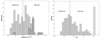 |
Fig. 1. Distribution of neutral hydrogen column density log(NH) (left panel) and hardness ratios (HRs; right panel) for AGNs selected using the MEx diagram. Objects that do not show absorption are plotted at HR = 1, and are represented with a solid line histogram in the left panel. The dotted vertical lines at log(NH) = 22 and HR = −0.2 indicate the adopted dividing lines between obscured and unobscured AGNs. |
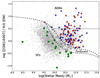 |
Fig. 2. Mass-excitation diagram. Grey dots represent galaxies in the zCOSMOS survey with ASPIC spectral-line measurements. The regions marked with dashed lines show the location of AGNs, composites, and star-forming galaxies. Grey circles represent X-ray sources, and red and blue circles represent obscured and unobscured AGNs with X-ray emission. Green circles denote X-ray-detected sources identified as star-forming galaxies. The dotted horizontal line at y = 0.5 shows the separation between high- and low-excitation AGNs. |
We compared stellar masses from different methods in the COSMOS2015 and COSMOS2020 catalogues and found no significant differences. Thus, we adopted the COSMOS2015 MASS_BEST values, derived from spectral fitting techniques. Open circles represent sources with X-ray emission, while red and blue circles represent obscured and unobscured AGNs according to hydrogen column-density estimates. Dashed lines show the separation criterion among AGNs, composites, and star-forming galaxies taken from Juneau et al. (2014). We also include the demarcation (horizontal dotted line at y = 0.5) that allows the separation between high-and low-excitation AGNs from Kewley et al. (2006). We find 17 and 13 obscured and unobscured AGNs with high-excitation values (log([O III]λ5007/Hβ) ≥ 0.5).
It is also noticeable that some X-ray-emitting sources lie in the region of the MEx diagram typically populated by star-forming galaxies. A possible explanation for their X-ray emission could be the presence of high-mass X-ray binaries (HMXBs). Mineo et al. (2012) analysed a sample of nearby galaxies hosting HMXB populations and found a correlation between the star formation rate (SFR) and the X-ray luminosity, described by the relation LX ≈ 2.6 × 1039 × SFR [erg s−1]. If the sources in the MEx diagram were powered solely by HMXBs, this would imply extremely high star formation rates of the order of 103–104 M⊙ yr−1, which are atypical for such systems (see Figure 3). An alternative explanation is that these sources are optically dull AGNs – that is, weakly accreting active nuclei with truncated accretion discs – likely associated with radiatively inefficient accretion flows (Trump et al. 2009).
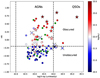 |
Fig. 3. Hardness ratio as function of hard (2–10 keV) X-ray luminosity. Vertical dashed lines show the typical separation for AGNs and quasars used in the X-rays. The horizontal line shows the limit values for obscured and unobscured AGNs in the X-rays. Stars and ‘X’ symbols indicate obscured and unobscured AGNs with high-excitation values (log([O III]λ5007/Hβ) > 0.5). Sources marked with green circles correspond to X-ray emitters found in the region of the MEx diagram that is generally associated with star-forming galaxies. Vertical colour bar shows the corresponding log(NH) values. |
4. AGN properties
4.1. Redshift and stellar-mass distributions
We find that obscured and unobscured AGNs have similar redshift distributions, with mean values of zobs = 0.74 ± 0.11 and zunobs = 0.74 ± 0.10, respectively. Similarly, their stellar mass distributions are comparable, with mean values of log10(massobs)=10.7 ± 0.3 and log10(massunobs)=10.8 ± 0.3 (M⊙). A Kolmogorov-Smirnov (K-S) null probability test confirms that the two samples of obscured and unobscured AGNs are statistically indistinguishable, with a null probability of pK-S = 0.18. We did not differentiate between low- and high-excitation AGNs for this analysis.
4.2. Hardness ratio and X-ray luminosity
In this section, we examine the relationship between the X-ray hardness ratio and luminosity, providing insights into how absorption and intrinsic emission characteristics differentiate AGN populations. Figure 3 presents the hardness ratio versus the hard (2–10 keV) X-ray luminosity for obscured and unobscured AGNs. The vertical colour bar indicates the logarithm of the hydrogen column density (log(NH). Highly excited obscured and unobscured AGNs are marked with stars and X symbols, respectively. The vertical dashed line separates objects with log(X-ray) > 44, typically associated with quasars, from those with log(X-ray) < 44, which are more commonly classified as AGNs.
A clear trend emerges: high-excitation AGNs, both obscured and unobscured, tend to exhibit higher HR values compared to low-excitation AGNs. Highly excited AGNs are often associated with relatively high accretion rates or powerful radiation fields, which generate strong optical emission lines, such as [O III]λ5007. This intense activity also leads to significant X-ray emission in both the soft and hard bands, contributing to the high HR values observed. For obscured AGNs, the surrounding gas and dust torus can absorb soft X-rays more effectively than hard X-rays, resulting in a higher HR value. However, the fact that even highly excited unobscured AGNs have large HR values suggests that their intrinsic X-ray emission is inherently hard. This could be linked to higher accretion rates or specific properties of the accretion flow around the black hole.
4.3. Ionisation parameter versus X-ray luminosity
The ionisation state of AGNs is strongly influenced by their central energy output, making the relationship between the ionization-sensitive O32 ratio and X-ray luminosity a key probe of AGN activity. Investigating this connection allowed us to explore how radiation from the accretion disc affects the surrounding narrow-line region. Figure 4 shows the ionisation-level sensitive O32 as a function of X-ray luminosity. AGNs with high-excitation values, both obscured and unobscured, are marked with ‘X’ symbols. Vertical dashed lines indicate the typical separation between AGNs and quasars used in X-ray luminosity (Treister et al. 2009), while horizontal lines highlight sources with high ionisation (O32 > 4) (Paalvast et al. 2018). We address these high ionisation sources in detail in the following sections. The red and blue lines represent linear fits to the obscured and unobscured AGN samples, respectively, without distinguishing between low- and high-excitation AGNs. We performed a linear regression analysis (without making any distinction between the different AGN types) to determine the relationship between the O32 parameter and X-ray luminosity: log(O32) = a × [log(LX)−42.5]+b.
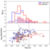 |
Fig. 4. Ionisation-level sensitive [O III]λ5007/[O II]λ3727 ratio as function of X-ray luminosity for the different AGN samples. Symbols are the same as in Figure 3. High-excitation obscured and unobscured AGNs are marked with ‘X’ symbols. Vertical dashed lines show the typical separation for AGNs and quasars used in the X-rays, and the horizontal lines show the limit for sources with high-ionisation values. |
For obscured AGNs, we found a = (0.20 ± 0.08), b = −0.28 ± 0.08, and a Pearson coefficient of R = 0.341. For unobscured AGNs, the corresponding values are a = (0.48 ± 0.09), b = ( − 0.19 ± 0.07), and a Pearson coefficient of 0.62. These results indicate a stronger and more pronounced correlation between X-ray luminosity and ionisation parameter for unobscured AGNs, consistent with a less absorption-affected close central engine environment. In contrast, obscured AGNs exhibit a weaker relationship, suggesting that the absorbing material plays a significant role in modulating high-energy radiation and, consequently, the ionisation state of the surrounding gas. The upper panel of Figure 4 shows the X-ray luminosity distributions for the different AGN samples. We find the following mean log(X-ray luminosity) values: obs_low = 43.30 ± 0.40, obs_high = 43.80 ± 0.60, and unobs_low = 43.10 ± 0.40, unobs_high = 43.40 ± 0.50. These results suggest that obscured, high-excitation AGNs tend to have higher X-ray luminosities on average.
An alternative explanation for these spectral characteristics is that these objects are optically ’dull’ AGNs, which are thought to host radiatively inefficient accretion flows (RIAFs; Trump et al. 2009). These flows produce fewer ionising photons compared to standard accretion discs, leading to a reduced ionisation level in the narrow-line region. Consequently, this results in lower [O III]λ5007/[O II]λ3727 ratios (Ho 2008), consistent with such AGNs harbouring inefficiently radiating central engines.
4.4. Obscured and unobscured AGNs according to the ionisation-level parameter
In this section, we investigate the different AGN samples according to the ionisation-level O32 ratio. Distinguishing between obscured and unobscured AGNs based on ionisation diagnostics provides deeper insight into the physical conditions of the NLR. The O32 ratio serves as an important tracer of ionisation levels, enabling a comparative analysis of AGNs with different levels of obscuration. Figure 5 (left panel) presents the MEx diagram for obscured (open circles) and unobscured (open triangles) AGNs. The vertical colour bar indicates the ionisation-level values. In the right panel, we include the ionisation-level O32 ratio distributions for the different AGN samples. Red and blue solid line histograms represent low-excitation obscured and unobscured X-ray AGNs (log([O III]λ5007/Hβ < 0.5), respectively. Red and blue dashed line histograms show the corresponding distributions for high-excitation AGNs (log([O III]λ5007/Hβ ≥ 0.5). The grey histogram represents MEx-selected AGNs without X-ray emission, matched in redshift and stellar mass to the X-ray AGN sample. We find the following mean O32 values: obs_low = −0.21 ± 0.27, obs_high = 0.17 ± 0.20, unobs_low = 0.13 ± 0.37, and unobs_high = 0.15 ± 0.31. For MEx-selected AGNs without X-ray emission and with similar redshift and stellar-mass values we find agn_noXrays= −0.05±0.30.
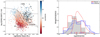 |
Fig. 5. Left panel: Mass-excitation diagram for sample of galaxies in the zCOSMOS survey with ASPIC spectral-line measurements. Obscured AGNs with X-ray emission are plotted with open circles, and the unobscured sample is shown with open triangles. The dashed and dotted lines demarcate the same regions as those in Figure 2. Vertical colour bar shows the ionisation-level [O III]λ5007/[O II]λ3727 ratio values. Right panel: Ionisation-level [O III]λ5007/[O II]λ3727 ratio distributions for the different AGN samples. Red and blue solid line histograms represent the distribution for obscured and unobscured X-ray AGNs with low-excitation values. High-excitation AGNs are plotted with dashed line distributions that represent the kernel density estimates (KDEs) for obscured and unobscured X-ray AGNs. We also plot the individual observations with marginal ticks. |
High-excitation obscured and unobscured AGNs, along with low-excitation unobscured AGNs, exhibit similar O32 values (mean values ∼0.15 dex). However, low-excitation obscured AGNs show a significantly lower O32 value, differing by approximately 0.36 dex. An analysis of variance (ANOVA; Fisher 1925) confirms that the mean differences across the four defined groups (obscured-unobscured × high-low excitation) are statistically significant (p < 10−7). Post hoc comparisons using the Tukey honestly significant difference test Tukey (1949) show that the obscured, low-excitation AGNs have systematically lower O32 values than the other three groups, which do not differ significantly among themselves. These results suggest that low-excitation obscured AGNs may represent a physically distinct population, possibly characterised by lower ionisation parameters or different narrow-line region conditions. This is consistent with studies suggesting that obscured AGNs often experience a decrease in the ionisation parameter due to the presence of gas or dust in the near-nuclear environment (Dempsey & Zakamska 2018; Lu et al. 2019). Alternatively, the observed trends may indicate that the ionization conditions in the NLR are not solely determined by AGN obscuration, but also reflect differences in host-galaxy properties or AGN structure. The lack of a clear separation between obscured and unobscured AGNs in the high-excitation regime suggests that additional physical parameters such as gas density, metallicity, or ionising photon flux may play a more dominant role in setting the ionisation state in these systems.
4.5. Star formation rate
The interplay between AGN activity and star formation is a fundamental aspect of galaxy evolution. By examining the star formation rates (SFRs) of AGN host galaxies, we can investigate whether AGN-driven feedback influences ongoing star formation, particularly in the context of obscured and unobscured sources. We calculated the SFR using the estimator proposed by Maier et al. (2009):
![Mathematical equation: $$ \begin{aligned} {\log }[\mathrm{SFR}/M_{\odot }\,\mathrm{yr}^{-1}]={\log }[L_{[\mathrm {OII}]}/(\mathrm{ergs\,s}^{-1})]- 41 - 0.195 \times M_{\rm B} - 3.434 ,\end{aligned} $$](/articles/aa/full_html/2025/09/aa54599-25/aa54599-25-eq1.gif) (1)
(1)
where L[O II] is the luminosity of the [O II]λ3727 line and MB is the absolute B-band magnitude. Figure 6 (left panel) presents the MEx diagram for the sample of galaxies and AGNs. The vertical colour bar indicates the SFR values calculated using Equation 1. The right panel shows the SFR distribution for the AGN sample. We find the following mean values: obs_low = 0.24 ± 0.53, unobs_low = 0.28 ± 0.46, obs_high = 0.75 ± 0.52, unobs_high = 0.68 ± 0.57, and the sample of AGN selected according with the MEx diagram without X-ray emission: noX = −0.015 ± 0.5. As shown, both obscured and unobscured AGNs with high-excitation values exhibit higher SFRs compared to low-excitation AGNs. Objects with high O32 values (> 0.6), as shown in Figure 4, also tend to have high SFRs (with values of the order of 1 calculated using Formula 1), suggesting a connection between high ionisation and active star formation in these AGNs. We performed Welch’s t-test (Welch 1947) to compare the distributions between obscured and unobscured sources within the low- and high-excitation groups. Welch’s test was chosen because it accounts for unequal variances and sample sizes between groups, providing a more reliable comparison under these conditions. No statistically significant differences were found between obscured and unobscured samples in either excitation regime (p > 0.7). In contrast, significant differences emerge when comparing low- and high-excitation sources within both obscured (p = 0.0023) and unobscured (p = 0.036) groups. These findings indicate that the excitation level, rather than obscuration, is the main factor influencing the observed variations in the analysed parameter. Similar results were published by Nakajima & Ouchi (2014) in a sample of galaxies with z = 2–3; the authors found that galaxies with large O32 values are associated with less massive galaxies with efficient star formation.
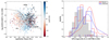 |
Fig. 6. Left panel: MEx diagram for sources in zCOSMOS and ASPIC catalogues. The vertical colour bar represents the SFR values obtained using the formula of Maier et al. (2009) from [O II] luminosity and MB magnitudes. AGNs are represented as in previous figures. Right panel: SFR distribution for different AGN samples. Colour-code and histogram lines are the same as in previous figures. |
4.6. O32 and R23 parameters
Pagel et al. (1979) first introduced the R23 parameter, defined as R23 = ([O III]λ5007+[O II]λ3727)/Hβ, to study the properties of HII regions in nearby galaxies. This parameter has since been widely used in the literature. R23 is sensitive to metallicity, exhibiting a biphasic behaviour. For low-metallicity galaxies, R23 increases with metallicity until it reaches a maximum just under solar abundance (Curti et al. 2017; Nakajima et al. 2022). However, for high-metallicity galaxies, R23 decreases as the gas-phase O/H ratio increases. This occurs because oxygen, an efficient coolant, reduces the gas temperature, leading to fewer collisionally excited oxygen ions and weaker oxygen emission lines (Perrotta et al. 2021). This phenomenon, known as the double-value degeneracy (Curti et al. 2020), means that the same R23 value can be obtained for two different metallicity values.
Figure 7 shows the MEx diagram (left panel) and the corresponding R23 distribution (right panel) for the AGN samples. Low-excitation obscured AGNs exhibit higher R23 values (0.64–0.5 = 0.14 dex) compared to the unobscured AGNs. Both obscured and unobscured high-excitation AGNs show similar R23 distributions (around 1.05 and 1.07 dex). A high R23 value often indicates a strong ionising radiation field in the AGN’s surrounding region. In such environments, oxygen is in higher ionisation states ([O III] and [O II]), suggesting that the AGN’s radiation is energetic enough to efficiently ionise the gas. This is typical of AGNs with a highly active accretion disc or powerful central source. In some cases, high R23 values are associated with low metallicity in the surrounding gas. In low-metallicity regions, fewer heavy metals are available to cool the gas radiatively, allowing the ionised oxygen lines to be more prominent relative to Hβ. We performed Welch’s t-tests (Welch 1947) to compare the analysed parameter between different groups, accounting for unequal variances and sample sizes. Significant differences were found when comparing high- and low-excitation sources within both obscured (t = 6.76, p < 0.001) and unobscured (t = 7.37, p < 0.001) samples. Additionally, a significant difference was observed between obscured and unobscured sources in the low-excitation regime (t = 2.85, p = 0.006). In contrast, no statistically significant difference was found between obscured and unobscured sources in the high-excitation group (t = −0.19, p = 0.85). These results reinforce the conclusion that the excitation level predominantly influences the observed variations, with obscuration playing a less significant role, particularly in the high-excitation regime.
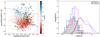 |
Fig. 7. Left panel: MEx diagram for sources identified in zCOSMOS and ASPIC catalogues. The vertical colour bar shows the log(R23) parameter values. Right panel: Distribution of log(R23) values for same AGN samples as in Figure 5. |
Active galactic nuclei with high R23 values may reside in environments with lower metallicity, possibly due to gas accretion from the circumgalactic or the intergalactic medium. In general, galaxies with high R23 and log([O III]λ5007/Hβ) > 0.5 are indicative of metal-poor environments and significant stellar activity, making them intriguing objects for studying galactic evolution and star formation processes.
The O32 versus R23 diagram is a useful tool for investigating the metallicity and ionisation state in the local Universe and up to z = 2 − 3 (Kewley & Dopita 2002; Nakajima & Ouchi 2014). Figure 8 shows the O32 parameter plotted against the R23 parameter for obscured and unobscured AGNs. High-excitation AGNs are marked with ‘X’ symbols. We also plot the corresponding values of extreme emission-line galaxies (z < 0.9) from the zCOSMOS survey (Amorín et al. 2015) (golden open squares). We correlated the Amorín et al. (2015) sample of galaxies with the spectral-line measurements from the ASPIC catalogue and have taken into account the same definitions used in our AGN samples (0.5 < z < 0.9 and same cuts in the equivalent widths in the [O III]λ5007, [O II]λ3727and Hβ lines). Open circles and triangles in purple and dark green show the distribution of galaxies with 0.3 < z < 1 in the Great Observatories Origins Deep Survey–North (GOODS-N) field with high (12+log(O/H) > 8.8) and low (8.5 < 12+log(O/H) < 8.8) metallicity values (Kobulnicky & Kewley 2004). We also plot a sample of high-redshift galaxies (4 < z < 6) with 12+log(O/H) < 8.5, identified in the JWST/NIRSpec survey (filled circles in light green; Nakajima et al. (2023)) Grey contours show the corresponding distribution for MEx-selected AGNs without X-ray emission with the same redshift and stellar-mass limits as our AGN sample. A statistical analysis using Student’s t-test reveals that the values of log(R23) show a significant difference between the samples of AGNs without X-ray emission and the obscured and unobscured AGNs. In contrast, according to the same statistical analysis, the values of log(O32) between the different samples do not show a significant difference, and the null hypothesis of equal means is not rejected. A group of high-excitation obscured and unobscured AGNs exhibit high R23 values (log(R23) > 1) and relatively low O32 values. This is indicative of galaxies in more advanced stages of chemical evolution, where there is sufficient oxygen present, but the ionising radiation is not energetic enough to sustain a high proportion of doubly ionised oxygen. In summary, this combination suggests that galaxies, although oxygen-rich, high R23, and possibly originating in actively forming stars (Curti et al. 2017; Jiang et al. 2019), do not experience extreme ionisation conditions, resulting in moderate-to-low O32 values, likely due to lower metallicity or less intense UV radiation.
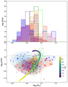 |
Fig. 8. Line-ratio diagnostic diagram of R23 = ([O III]λ5007+[O II]λ3727)/Hβ versus O32 = [O III]λ5007/[O II]λ3727). Obscured and unobscured AGNs are plotted with the same symbols as in the previous figures. Purple open circles and dark green triangles represent galaxies with high (12+log(O/H) > 8.8) and low (12+log(O/H) < 8.8) metallicity taken from Kobulnicky & Kewley (2004). Golden open squares represent the corresponding values for extreme emission-line galaxies out to z ∼ 1 in the zCOSMOS survey (Amorín et al. 2015). Light green filled circles represent high-redshift galaxies (4 < z < 6) with 12+log(O/H) < 8.5 from the JWST/NIRSpec survey (Nakajima et al. 2023). Grey contours show the corresponding distribution for MEx-selected AGNs without X-ray emission with the same redshift and stellar-mass limits as our AGN sample. The strong line diagnostic curve indicates the colour-coded metallicity values in solar units (Z/Z⊙) taken from Curti et al. (2017). |
4.7. Specific black-hole accretion rates, λsBHAR, obscuration, and metallicity
In the context of galactic evolution, SMBHs play a crucial role, particularly during active growth phases characterised by the accretion of material from their surroundings. This accretion process, along with the emission of large amounts of electromagnetic radiation from the accretion disc, is a characteristic feature of AGNs (Yang et al. 2018).
A key parameter for understanding the relationship between SMBHs and their host galaxies is the specific black-hole accretion rate (λsBHAR). This parameter, which quantifies the ratio of the black-hole accretion rate to the stellar mass of the galaxy, allows us to explore how accretion processes relate to the global properties of host galaxies (López et al. 2023). More specifically, λsBHAR provides insight into the efficiency with which SMBHs consume material relatively to the total stellar mass of the galaxy (Mountrichas et al. 2022, 2024).
We define λsBHAR in dimensionless units as
 (2)
(2)
where LX is the rest-frame 2–10 keV X-ray luminosity, kbol is a bolometric correction factor (we adopted a constant kbol = 25, as in Aird et al. (2018), Mountrichas et al. (2022, 2024) and ℳ* is the total stellar mass of the AGN host galaxy estimated from SED fitting. The significance of λsBHAR lies in its ability to directly compare accretion activity between galaxies of different masses, mitigating biases related to galaxy size or total stellar mass. A high λsBHAR indicates that the black hole is in an active growth phase, often associated with the luminous AGNs, while a low value suggests lower accretion, typical of obscured AGNs or less active phases (Mountrichas et al. 2024).
Figure 9 illustrates the correlation between λsBHAR and the hydrogen column density, NH. Filled red and blue circles represent low-excitation obscured and unobscured AGNs, respectively. AGNs with high-excitation values are marked with X symbols (left panel). In the right panel, we plot the distribution of λsBHAR for the different AGN samples. We find the following mean log(λsBHAR) values: un_low = −1.65, un_high = −1.26, obs_low = −1.49, and obs_high = −1.01. We find a weak but positive trend line between log(λsBHAR) and log(NH). The following linear regression was obtained without differentiating between the various AGN types: log(λsBHAR) = (0.18 ± 0.05) × (log(NH)−20) − (1.8 ± 0.1). However, the weak Pearson correlation coefficient (R = 0.31) suggests a limited direct dependence between the two variables. It would seem that the trend might be driven primarily by three Compton-thick AGNs (log(NH > 24). For this reason, we evaluated the influence of the three Compton-thick AGNs. When we excluded the three Compton-thick sources, the correlation weakens significantly to R = 0.16, and the regression becomes
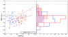 |
Fig. 9. Specific black-hole accretion rate λsBHAR as a function of hydrogen column density, log(NH), for obscured and unobscured AGNs. Low (high) excitation obscured and unobscured AGNs are plotted with solid (Xs) red and blue circles. The dashed black line indicates the minimum detectable λsBHAR as a function of log(NH) for a fixed stellar mass of log(M*/M⊙)=10.5 and a mean redshift of z = 0.75. This detection limit accounts for the hard-band (2–10 keV) flux threshold and includes attenuation due to obscuration; this was estimated using an empirical transmission model. Sources lying below this line are likely to fall below the detection limit of the X-ray survey. In the right panel, we plot the corresponding distribution of λsBHAR for the different AGN samples. Solid red and blue distributions represent obscured and unobscured AGNs, while red dashed line and blue dotted line histograms correspond to high-excitation obscured and unobscured AGNs, respectively. |

These results indicate that a small number of highly obscured sources may drive the apparent positive trend, which becomes less significant when they are removed. Nevertheless, the slope remains positive, suggesting a possible, although tentative, connection between obscuration and black-hole accretion activity. To further assess the impact of selection effects, we estimated the minimum detectable λsBHAR as a function of NH, assuming a stellar mass of log(M*/M⊙)=10.5 and a redshift of z = 0.75, which are representative values for our sample. This limit, indicated by a dashed line in Figure 9, incorporates an attenuation correction derived from the torus model (Murphy & Yaqoob 2009) and the observed hard-band flux limit. We find that most Compton-thick AGNs (log(NH)> 24) lie near this threshold, suggesting that some heavily obscured sources with lower accretion rates may fall below the detection limit. However, the detection of several such sources above this boundary indicates that the observed positive trend between λsBHAR and NH cannot be entirely attributed to selection bias.
It is reasonable to hypothesise a negative correlation between obscuration (as measured by NH) and the black-hole accretion rate, meaning that less obscured AGNs should exhibit higher accretion rates. This expectation is consistent with the findings of Vijarnwannaluk et al. (2024), who compared NH values with the Eddington ratio, which is often used as a proxy for λBHAR (López et al. 2023; Mountrichas et al. 2024). Similar results were obtained by Laloux et al. (2024), who found that unobscured AGNs exhibit a systematic offset towards higher a Eddington ratio compared to their obscured counterparts. However, a positive correlation between these parameters has also been reported in some studies, such as those by Lanzuisi et al. (2015), Barchiesi et al. (2024). A higher accretion rate may be associated with an increased hydrogen column density, particularly if the surrounding material is denser or located closer to the black hole. This could result in stronger obscuration, although the exact nature of this relationship may depend on the AGN geometry, the distribution of the surrounding material, and other factors (Buchner et al. 2015).
Figure 10, left panel, plots λsBHAR against the R23 parameter. Both obscured and unobscured high-excitation AGNs (marked with X symbols) exhibit lower metallicities, as indicated by the R23 parameter. We find a weak (or marginal) positive correlation between these two quantities, although the scatter remains significant. We obtained the following linear regression (considering all AGN types together) for the relationship between λsBHAR and the R23 parameter: log(λsBHAR)=0.60 × log(R23)−1.83 with a Pearson coefficient R = 0.34.
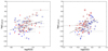 |
Fig. 10. Specific black-hole accretion rate, λsBHAR, as function of R23 (left panel) and O32 (right panel) parameters for the different AGN samples. The plotted symbols are the same as those in Figure 9. Objects without error bars correspond to sources for which the uncertainty in the Hβ emission line is not available. Points enclosed by large circles represent sources with log(R23) > 1. |
The correlation between the R23 parameter and λsBHAR may provide insights into how black-hole accretion activity is influenced by the chemical environment of the host galaxy. In general, higher metallicity is expected to be associated with a lower specific accretion rate, as more metal-rich galaxies tend to have less gas available for accretion. Although Du et al. (2014), for example, did not find a correlation between metallicity estimated through the ratio of certain emission lines and the accretion rate of black holes, these authors found that neither the BLR nor the NLR metallicity correlates with black-hole masses or Eddington ratios. However, they reported a strong correlation between NLR and BLR metallicities.
In the right panel of Figure 10, we plot the λsBHAR versus O32 ionisation-level parameter. As can be seen, we find a weak but positive correlation between these two parameters. The linear regression is log(λsBHAR) = 0.66×log(O32)−1.45, and the Pearson correlation coefficient R = 0.42. As in previous cases, we did not make any distinction between the different AGN types. We mark sources with log(R23) > 1 with open circles. These objects are above the linear relationship, indicating that, on average, they have large black-hole accretion rates. No significant trend was observed when comparing obscured and unobscured AGNs as well as high- and low-excitation sources in our sample. This may be because the O32 parameter measures the ionisation in the narrow-line region, which is located on a larger scale than the obscuring region of the torus. If the ionising radiation from the AGN can escape in a similar manner in both cases (obscured and unobscured), the O32 value would not be affected by the obscuration measured from NH.
5. Summary and discussions
In this study, we analysed the properties of X-ray-selected AGNs based on the MEx diagram. We categorised AGNs into obscured and unobscured sources using hydrogen column density estimates (log(NH) = 22) and into high- and low-excitation regimens using the [O III]λ5007/Hβ ratio of 0.5 as a threshold. We investigated various AGN properties, including X-ray luminosity, stellar mass, hardness ratio, specific black-hole accretion rate (λsBHAR), and emission-line ratios such as [O III]λ5007/[O II]λ3727 and R23. Our main findings are listed below.
-
High-excitation AGNs: Both obscured and unobscured high-excitation AGNs exhibit larger hardness ratios compared to low-excitation AGNs. This suggests that these AGNs are associated with more active nuclei and higher accretion rates, where the surrounding gas plays a crucial role in both X-ray absorption and optical line excitation.
-
Ionisation and X-ray luminosity: Unobscured AGNs show a stronger correlation between the [O III]λ5007/[O II]λ3727 ratio and X-ray luminosity compared to obscured AGNs. Additionally, high-excitation obscured AGNs tend to have higher X-ray luminosities on average. These findings suggest that obscured and highly excited AGNs are associated with more active nuclei or higher accretion rates.
-
Ionisation levels: High-excitation obscured and unobscured AGNs, along with low-excitation unobscured AGNs, have similar [O III]λ5007/[O II]λ3727 ratios. However, low-excitation obscured AGNs exhibit significantly lower values, potentially due to obscuration blocking ionising radiation from the central engine or different physical conditions in the broad-line region.
-
Metallicity and ionisation: Both highly excited obscured and unobscured AGNs tend to have larger R23 values, indicating lower metallicities in their host galaxies. A fraction of high-excitation AGNs exhibit extremely low metallicity values, similarly to high-redshift galaxies observed with JWST.
-
Accretion rate and obscuration: We find a positive correlation between λsBHAR and NH, suggesting that obscuration may be related to specific phases of rapid black-hole growth. However, there is no clear relationship between high-excitation obscured and unobscured sources, implying that AGNs in active accretion phases may undergo episodes of obscuration and unobscuration.
-
Accretion, metallicity and ionisation: AGNs with high R23 values and high excitation are associated with low-metallicity environments. Higher metallicity is expected to correspond to a lower specific accretion rate, as metal-rich galaxies typically have less gas available for accretion. These findings provide valuable insights into the ionisation properties and environmental conditions of AGNs, shedding light on the physics of active nuclei under various obscuration and excitation scenarios. The results highlight the importance of the surrounding environment in modulating the observed properties of AGNs and suggest that obscuration and excitation are closely linked to physical processes such as X-ray absorption, accretion rate, and the chemical composition of the medium. The observed differences between various types of AGNs, including obscured and unobscured sources (as well as those with high or low excitation) and with their properties such as metallicity, ionisation state, and black-hole accretion rate, can be explained as deviations within the unified models. In this context, the size of the torus in particular may play a decisive role in determining these classifications. Several studies have proposed modifications to the unified model of AGNs. For instance, Goulding et al. (2012) analysed a sample of heavily obscured local AGNs –specifically, Compton-thick sources with NH > 1.5 × 1024 cm−2– and suggested that the primary contributor to the observed mid-IR dust extinction is not the torus, but dust located at much larger scales within the host galaxy. This interpretation aligns with previous findings by other authors (Malkan et al. 1998; Matt 2000; Guainazzi et al. 2001; Goulding & Alexander 2009; Sokol et al. 2023). Our findings support an evolutionary scenario where obscured sources accrete more rapidly due to the availability of gas in their surroundings (Di Matteo et al. 2005; Sanders et al. 2007; Hopkins et al. 2008a,b; Ricci et al. 2021). These studies are crucial for understanding the complex interplay between AGNs and their host galaxies, as well as the feedback processes that regulate star formation and galaxy evolution in the Universe (Hickox & Alexander 2018; Maiolino & Mannucci 2019).
The catalogue can be downloaded from ftp://ftp.iap.fr/pub/from_users/hjmcc/COSMOS2015/
The catalogue can be downloaded from https://data.lam.fr/aspic/retrieve-aspic-data/download
Acknowledgments
We thank the anonymous referee for his/her useful comments and suggestions. This work was partially supported by the Consejo Nacional de Investigaciones Científicas y Técnicas (CONICET) and the Secretaría de Ciencia y Tecnología de la Universidad Nacional de Córdoba (SeCyT). Based on data products from observations made with ESO Telescopes at the La Silla Paranal Observatory under ESO programme ID 179.A-2005 and on data products produced by TERAPIX and the Cambridge Astronomy Survey Unit on behalf of the UltraVISTA consortium. Based on zCOSMOS observations carried out using the Very Large Telescope at the ESO Paranal Observatory under Programme ID: LP175.A-0839 (zCOSMOS). This research has made use of the VizieR catalogue access tool, CDS, Strasbourg, France (DOI: http://dx.doi.org/10.26093/cds/vizier). This research has made use of the ASPIC database, operated at CeSAM/LAM, Marseille, France. Software: Matplotlib (Hunter 2007), NumPy (van der Walt et al. 2011; Harris et al. 2020).
References
- Aird, J., Coil, A. L., Moustakas, J., et al. 2012, ApJ, 746, 90 [CrossRef] [Google Scholar]
- Aird, J., Coil, A. L., & Georgakakis, A. 2018, MNRAS, 474, 1225 [NASA ADS] [CrossRef] [Google Scholar]
- Alexander, D. M., & Hickox, R. C. 2012, New Astron. Rev., 56, 93 [Google Scholar]
- Alonso-Herrero, A., Ramos Almeida, C., Mason, R., et al. 2011, ApJ, 736, 82 [NASA ADS] [CrossRef] [Google Scholar]
- Ambartsumian, V. A. 1958, Izvestiya Akademiya Nauk Armyanskoi, 11, 9 [Google Scholar]
- Amorín, R., Pérez-Montero, E., Contini, T., et al. 2015, A&A, 578, A105 [NASA ADS] [CrossRef] [EDP Sciences] [Google Scholar]
- Antonucci, R. 1993, ARA&A, 31, 473 [Google Scholar]
- Arnouts, S., & Ilbert, O. 2011, LePHARE: Photometric Analysis for Redshift Estimate, Astrophysics Source Code Library [record ascl:1108.009] [Google Scholar]
- Assef, R. J., Kochanek, C. S., Ashby, M. L. N., et al. 2011, ApJ, 728, 56 [NASA ADS] [CrossRef] [Google Scholar]
- Audibert, A., Riffel, R., Sales, D. A., Pastoriza, M. G., & Ruschel-Dutra, D. 2017, MNRAS, 464, 2139 [NASA ADS] [CrossRef] [Google Scholar]
- Baldwin, J. A., Phillips, M. M., & Terlevich, R. 1981, PASP, 93, 5 [Google Scholar]
- Barchiesi, L., Vignali, C., Pozzi, F., et al. 2024, A&A, 685, A141 [NASA ADS] [CrossRef] [EDP Sciences] [Google Scholar]
- Bassett, R., Ryan-Weber, E. V., Cooke, J., et al. 2019, MNRAS, 483, 5223 [Google Scholar]
- Beifiori, A., Courteau, S., Corsini, E. M., & Zhu, Y. 2012, MNRAS, 419, 2497 [NASA ADS] [CrossRef] [Google Scholar]
- Bongiorno, A., Mignoli, M., Zamorani, G., et al. 2010, A&A, 510, A56 [NASA ADS] [CrossRef] [EDP Sciences] [Google Scholar]
- Bornancini, C., & García Lambas, D. 2020, MNRAS, 494, 1189 [Google Scholar]
- Bornancini, C. G., Oio, G. A., Alonso, M. V., & García Lambas, D. 2022, A&A, 664, A110 [NASA ADS] [CrossRef] [EDP Sciences] [Google Scholar]
- Brandt, W. N., & Alexander, D. M. 2015, A&A Rev., 23, 1 [NASA ADS] [CrossRef] [Google Scholar]
- Bruzual, G., & Charlot, S. 2003, MNRAS, 344, 1000 [NASA ADS] [CrossRef] [Google Scholar]
- Buchner, J., Georgakakis, A., Nandra, K., et al. 2014, A&A, 564, A125 [NASA ADS] [CrossRef] [EDP Sciences] [Google Scholar]
- Buchner, J., Georgakakis, A., Nandra, K., et al. 2015, ApJ, 802, 89 [Google Scholar]
- Buchner, J., Brightman, M., Nandra, K., Nikutta, R., & Bauer, F. E. 2019, A&A, 629, A16 [NASA ADS] [CrossRef] [EDP Sciences] [Google Scholar]
- Caputi, K. I. 2013, ApJ, 768, 103 [Google Scholar]
- Chang, Y.-Y., Le Floc’h, E., Juneau, S., et al. 2017, ApJS, 233, 19 [Google Scholar]
- Civano, F., Elvis, M., Brusa, M., et al. 2012, ApJS, 201, 30 [Google Scholar]
- Civano, F., Marchesi, S., Comastri, A., et al. 2016, ApJ, 819, 62 [Google Scholar]
- Comastri, A., Vignali, C., Brusa, M., Hellas, & Hellas2XMM Consortia, 2002, in IAU Colloq. 184: AGN Surveys, eds. R. F. Green, E. Y. Khachikian, & D. B. Sanders, ASP Conf. Ser., 284, 235 [Google Scholar]
- Curti, M., Cresci, G., Mannucci, F., et al. 2017, MNRAS, 465, 1384 [Google Scholar]
- Curti, M., Mannucci, F., Cresci, G., & Maiolino, R. 2020, MNRAS, 491, 944 [Google Scholar]
- Dempsey, R., & Zakamska, N. L. 2018, MNRAS, 477, 4615 [NASA ADS] [CrossRef] [Google Scholar]
- Dewangan, G. C., Mathur, S., Griffiths, R. E., & Rao, A. R. 2008, ApJ, 689, 762 [NASA ADS] [CrossRef] [Google Scholar]
- Di Matteo, T., Springel, V., & Hernquist, L. 2005, Nature, 433, 604 [NASA ADS] [CrossRef] [Google Scholar]
- Ding, X., Silverman, J., Treu, T., et al. 2020, ApJ, 888, 37 [NASA ADS] [CrossRef] [Google Scholar]
- Donley, J. L., Rieke, G. H., Pérez-González, P. G., Rigby, J. R., & Alonso-Herrero, A. 2007, ApJ, 660, 167 [Google Scholar]
- Donley, J. L., Rieke, G. H., Pérez-González, P. G., & Barro, G. 2008, ApJ, 687, 111 [NASA ADS] [CrossRef] [Google Scholar]
- Donley, J. L., Kartaltepe, J., Kocevski, D., et al. 2018, ApJ, 853, 63 [NASA ADS] [CrossRef] [Google Scholar]
- Du, P., Wang, J.-M., Hu, C., et al. 2014, MNRAS, 438, 2828 [NASA ADS] [CrossRef] [Google Scholar]
- Elitzur, M., & Ho, L. C. 2009, ApJ, 701, L91 [Google Scholar]
- Elitzur, M., & Shlosman, I. 2006, ApJ, 648, L101 [Google Scholar]
- Ferrarese, L., & Merritt, D. 2000, ApJ, 539, L9 [Google Scholar]
- Fisher, R. A. 1925, Statistical Methods for Research Workers (Edinburgh: Oliver and Boyd) [Google Scholar]
- Gebhardt, K., Bender, R., Bower, G., et al. 2000, ApJ, 539, L13 [Google Scholar]
- Georgantopoulos, I., & Georgakakis, A. 2005, MNRAS, 358, 131 [Google Scholar]
- Gilli, R., Daddi, E., Zamorani, G., et al. 2005, A&A, 430, 811 [NASA ADS] [CrossRef] [EDP Sciences] [Google Scholar]
- Goulding, A. D., & Alexander, D. M. 2009, MNRAS, 398, 1165 [NASA ADS] [CrossRef] [Google Scholar]
- Goulding, A. D., Alexander, D. M., Bauer, F. E., et al. 2012, ApJ, 755, 5 [Google Scholar]
- Graham, A. W., & Scott, N. 2015, ApJ, 798, 54 [Google Scholar]
- Granato, G. L., De Zotti, G., Silva, L., Bressan, A., & Danese, L. 2004, ApJ, 600, 580 [Google Scholar]
- Guainazzi, M., Fiore, F., Matt, G., & Perola, G. C. 2001, MNRAS, 327, 323 [Google Scholar]
- Häring, N., & Rix, H.-W. 2004, ApJ, 604, L89 [Google Scholar]
- Harris, C. R., Millman, K. J., van der Walt, S. J., et al. 2020, Nature, 585, 357 [NASA ADS] [CrossRef] [Google Scholar]
- Hasinger, G., Miyaji, T., & Schmidt, M. 2005, A&A, 441, 417 [NASA ADS] [CrossRef] [EDP Sciences] [Google Scholar]
- Hasinger, G., Capak, P., Salvato, M., et al. 2018, ApJ, 858, 77 [Google Scholar]
- Heckman, T. M., & Best, P. N. 2014, ARA&A, 52, 589 [Google Scholar]
- Hickox, R. C., & Alexander, D. M. 2018, ARA&A, 56, 625 [Google Scholar]
- Ho, L. C. 2008, ARA&A, 46, 475 [Google Scholar]
- Hogarth, L., Amorín, R., Vílchez, J. M., et al. 2020, MNRAS, 494, 3541 [NASA ADS] [CrossRef] [Google Scholar]
- Hopkins, P. F., Cox, T. J., Kereš, D., & Hernquist, L. 2008a, ApJS, 175, 390 [Google Scholar]
- Hopkins, P. F., Hernquist, L., Cox, T. J., & Kereš, D. 2008b, ApJS, 175, 356 [Google Scholar]
- Hsieh, B.-C., Wang, W.-H., Hsieh, C.-C., et al. 2012, ApJS, 203, 23 [NASA ADS] [CrossRef] [Google Scholar]
- Hunter, J. D. 2007, Comput. Sci. Eng., 9, 90 [NASA ADS] [CrossRef] [Google Scholar]
- Jiang, T., Malhotra, S., Rhoads, J. E., & Yang, H. 2019, ApJ, 872, 145 [NASA ADS] [CrossRef] [Google Scholar]
- Juneau, S., Dickinson, M., Alexander, D. M., & Salim, S. 2011, ApJ, 736, 104 [Google Scholar]
- Juneau, S., Bournaud, F., Charlot, S., et al. 2014, ApJ, 788, 88 [NASA ADS] [CrossRef] [Google Scholar]
- Kashino, D., Silverman, J. D., Sanders, D., et al. 2019, ApJS, 241, 10 [Google Scholar]
- Kauffmann, G., & Heckman, T. M. 2009, MNRAS, 397, 135 [NASA ADS] [CrossRef] [Google Scholar]
- Kewley, L. J., & Dopita, M. A. 2002, ApJS, 142, 35 [Google Scholar]
- Kewley, L. J., Groves, B., Kauffmann, G., & Heckman, T. 2006, MNRAS, 372, 961 [Google Scholar]
- Knobel, C., Lilly, S. J., Iovino, A., et al. 2012, ApJ, 753, 121 [Google Scholar]
- Kobulnicky, H. A., & Kewley, L. J. 2004, ApJ, 617, 240 [CrossRef] [Google Scholar]
- Kong, X., Cheng, F. Z., Weiss, A., & Charlot, S. 2002, A&A, 396, 503 [NASA ADS] [CrossRef] [EDP Sciences] [Google Scholar]
- Kormendy, J., & Ho, L. C. 2013, ARA&A, 51, 511 [Google Scholar]
- Koutoulidis, L., Georgantopoulos, I., Mountrichas, G., et al. 2018, MNRAS, 481, 3063 [NASA ADS] [CrossRef] [Google Scholar]
- Kriek, M., Shapley, A. E., Reddy, N. A., et al. 2015, ApJS, 218, 15 [NASA ADS] [CrossRef] [Google Scholar]
- Lacy, M., Storrie-Lombardi, L. J., Sajina, A., et al. 2004, ApJS, 154, 166 [Google Scholar]
- Lacy, M., Petric, A. O., Sajina, A., et al. 2007, AJ, 133, 186 [Google Scholar]
- Laigle, C., McCracken, H. J., Ilbert, O., et al. 2016, ApJS, 224, 24 [Google Scholar]
- Laloux, B., Georgakakis, A., Andonie, C., et al. 2023, MNRAS, 518, 2546 [Google Scholar]
- Laloux, B., Georgakakis, A., Alexander, D. M., et al. 2024, MNRAS, 532, 3459 [NASA ADS] [CrossRef] [Google Scholar]
- Lamareille, F., Contini, T., Le Borgne, J. F., et al. 2006, A&A, 448, 893 [NASA ADS] [CrossRef] [EDP Sciences] [Google Scholar]
- Lamareille, F., Brinchmann, J., Contini, T., et al. 2009, A&A, 495, 53 [NASA ADS] [CrossRef] [EDP Sciences] [Google Scholar]
- Lang, D., Hogg, D. W., & Mykytyn, D. 2016, The Tractor: Probabilistic astronomical source detection and measurement, Astrophysics Source Code Library [record ascl:1604.008] [Google Scholar]
- Lanzuisi, G., Ranalli, P., Georgantopoulos, I., et al. 2015, A&A, 573, A137 [NASA ADS] [CrossRef] [EDP Sciences] [Google Scholar]
- Lilly, S. J., Le Fèvre, O., Renzini, A., et al. 2007, ApJS, 172, 70 [Google Scholar]
- Lilly, S. J., Le Brun, V., Maier, C., et al. 2009, ApJS, 184, 218 [Google Scholar]
- López, I. E., Brusa, M., Bonoli, S., et al. 2023, A&A, 672, A137 [NASA ADS] [CrossRef] [EDP Sciences] [Google Scholar]
- Lu, K.-X., Zhao, Y., Bai, J.-M., & Fan, X.-L. 2019, MNRAS, 483, 1722 [NASA ADS] [CrossRef] [Google Scholar]
- Lynden-Bell, D. 1969, Nature, 223, 690 [NASA ADS] [CrossRef] [Google Scholar]
- Lynden-Bell, D., & Rees, M. J. 1971, MNRAS, 152, 461 [NASA ADS] [CrossRef] [Google Scholar]
- Magorrian, J., Tremaine, S., Richstone, D., et al. 1998, AJ, 115, 2285 [Google Scholar]
- Maier, C., Lilly, S. J., Zamorani, G., et al. 2009, ApJ, 694, 1099 [NASA ADS] [CrossRef] [Google Scholar]
- Maiolino, R., & Mannucci, F. 2019, A&A Rev., 27, 3 [NASA ADS] [CrossRef] [Google Scholar]
- Maiolino, R., Ruiz, M., Rieke, G. H., & Keller, L. D. 1995, ApJ, 446, 561 [Google Scholar]
- Malkan, M. A., Gorjian, V., & Tam, R. 1998, ApJS, 117, 25 [Google Scholar]
- Marchesi, S., Civano, F., Elvis, M., et al. 2016, ApJ, 817, 34 [Google Scholar]
- Martínez-Paredes, M., Aretxaga, I., Alonso-Herrero, A., et al. 2017, MNRAS, 468, 2 [Google Scholar]
- Marziani, P., D’Onofrio, M., Bettoni, D., et al. 2017, A&A, 599, A83 [NASA ADS] [CrossRef] [EDP Sciences] [Google Scholar]
- Matt, G. 2000, A&A, 355, L31 [NASA ADS] [Google Scholar]
- McConnell, N. J., & Ma, C.-P. 2013, ApJ, 764, 184 [Google Scholar]
- McLure, R. J., & Dunlop, J. S. 2000, MNRAS, 317, 249 [NASA ADS] [CrossRef] [Google Scholar]
- Merritt, D., & Ferrarese, L. 2001, MNRAS, 320, L30 [NASA ADS] [CrossRef] [Google Scholar]
- Messias, H., Afonso, J., Salvato, M., Mobasher, B., & Hopkins, A. M. 2012, ApJ, 754, 120 [Google Scholar]
- Miley, G., & De Breuck, C. 2008, A&A Rev., 15, 67 [NASA ADS] [CrossRef] [Google Scholar]
- Mineo, S., Gilfanov, M., & Sunyaev, R. 2012, MNRAS, 419, 2095 [Google Scholar]
- Mountrichas, G., & Georgantopoulos, I. 2024, A&A, 683, A160 [NASA ADS] [CrossRef] [EDP Sciences] [Google Scholar]
- Mountrichas, G., Buat, V., Yang, G., et al. 2022, A&A, 663, A130 [NASA ADS] [CrossRef] [EDP Sciences] [Google Scholar]
- Mountrichas, G., Viitanen, A., Carrera, F. J., et al. 2024, A&A, 683, A172 [NASA ADS] [CrossRef] [EDP Sciences] [Google Scholar]
- Murphy, K. D., & Yaqoob, T. 2009, MNRAS, 397, 1549 [Google Scholar]
- Mushotzky, R. 2004, in Supermassive Black Holes in the Distant Universe, ed. A. J. Barger, Astrophy. Space Sci. Lib., 308, 53 [Google Scholar]
- Nakajima, K., & Ouchi, M. 2014, MNRAS, 442, 900 [Google Scholar]
- Nakajima, K., Ouchi, M., Shimasaku, K., et al. 2013, ApJ, 769, 3 [NASA ADS] [CrossRef] [Google Scholar]
- Nakajima, K., Ouchi, M., Xu, Y., et al. 2022, ApJS, 262, 3 [CrossRef] [Google Scholar]
- Nakajima, K., Ouchi, M., Isobe, Y., et al. 2023, ApJS, 269, 33 [NASA ADS] [CrossRef] [Google Scholar]
- Netzer, H. 2015, ARA&A, 53, 365 [Google Scholar]
- Oke, J. B., & Gunn, J. E. 1983, ApJ, 266, 713 [NASA ADS] [CrossRef] [Google Scholar]
- Paalvast, M., Verhamme, A., Straka, L. A., et al. 2018, A&A, 618, A40 [NASA ADS] [CrossRef] [EDP Sciences] [Google Scholar]
- Padovani, P., Alexander, D. M., Assef, R. J., et al. 2017, A&A Rev., 25, 2 [NASA ADS] [CrossRef] [Google Scholar]
- Pagel, B. E. J., Edmunds, M. G., Blackwell, D. E., Chun, M. S., & Smith, G. 1979, MNRAS, 189, 95 [NASA ADS] [CrossRef] [Google Scholar]
- Perrotta, S., George, E. R., Coil, A. L., et al. 2021, ApJ, 923, 275 [Google Scholar]
- Ramos Almeida, C., & Ricci, C. 2017, Nat. Astron., 1, 679 [Google Scholar]
- Ramos Almeida, C., Levenson, N. A., Alonso-Herrero, A., et al. 2011, ApJ, 731, 92 [Google Scholar]
- Rees, M. J. 1974, The Observatory, 94, 168 [Google Scholar]
- Rees, M. J. 1984, ARA&A, 22, 471 [Google Scholar]
- Ricci, C., Privon, G. C., Pfeifle, R. W., et al. 2021, MNRAS, 506, 5935 [NASA ADS] [CrossRef] [Google Scholar]
- Sánchez, P., Lira, P., Cartier, R., et al. 2017, ApJ, 849, 110 [CrossRef] [Google Scholar]
- Sanders, D. B., Salvato, M., Aussel, H., et al. 2007, ApJS, 172, 86 [Google Scholar]
- Schmidt, M. 1963, Nature, 197, 1040 [Google Scholar]
- Schreiber, C., Glazebrook, K., Nanayakkara, T., et al. 2018, A&A, 618, A85 [NASA ADS] [CrossRef] [EDP Sciences] [Google Scholar]
- Scoville, N., Aussel, H., Brusa, M., et al. 2007, ApJS, 172, 1 [Google Scholar]
- Silverman, J. D., Kashino, D., Sanders, D., et al. 2015, ApJS, 220, 12 [NASA ADS] [CrossRef] [Google Scholar]
- Silverman, J. D., Mainieri, V., Ding, X., et al. 2023, ApJ, 951, L41 [NASA ADS] [CrossRef] [Google Scholar]
- Sokol, A. D., Yun, M., Pope, A., Kirkpatrick, A., & Cooke, K. 2023, MNRAS, 521, 818 [NASA ADS] [CrossRef] [Google Scholar]
- Springel, V., Di Matteo, T., & Hernquist, L. 2005a, MNRAS, 361, 776 [Google Scholar]
- Springel, V., White, S. D. M., Jenkins, A., et al. 2005b, Nature, 435, 629 [Google Scholar]
- Stern, D., Eisenhardt, P., Gorjian, V., et al. 2005, ApJ, 631, 163 [Google Scholar]
- Treister, E., Cardamone, C. N., Schawinski, K., et al. 2009, ApJ, 706, 535 [NASA ADS] [CrossRef] [Google Scholar]
- Tremonti, C. A., Heckman, T. M., Kauffmann, G., et al. 2004, ApJ, 613, 898 [Google Scholar]
- Trump, J. R., Impey, C. D., Taniguchi, Y., et al. 2009, ApJ, 706, 797 [Google Scholar]
- Tukey, J. W. 1949, Biometrics, 5, 99 [Google Scholar]
- Urrutia, T., Wisotzki, L., Kerutt, J., et al. 2019, A&A, 624, A141 [NASA ADS] [CrossRef] [EDP Sciences] [Google Scholar]
- Urry, C. M., & Padovani, P. 1995, PASP, 107, 803 [NASA ADS] [CrossRef] [Google Scholar]
- van der Walt, S., Colbert, S. C., & Varoquaux, G. 2011, Comput. Sci. Eng., 13, 22 [Google Scholar]
- Vijarnwannaluk, B., Akiyama, M., Schramm, M., et al. 2024, MNRAS, 529, 3610 [Google Scholar]
- Wandel, A. 1999, ApJ, 519, L39 [NASA ADS] [CrossRef] [Google Scholar]
- Weaver, J. R., Kauffmann, O. B., Ilbert, O., et al. 2022, ApJS, 258, 11 [NASA ADS] [CrossRef] [Google Scholar]
- Welch, B. L. 1947, Biometrika, 34, 28 [Google Scholar]
- Yang, G., Brandt, W. N., Vito, F., et al. 2018, MNRAS, 475, 1887 [NASA ADS] [CrossRef] [Google Scholar]
- Zhang, K., & Hao, L. 2018, ApJ, 856, 171 [NASA ADS] [CrossRef] [Google Scholar]
- Zou, F., Yang, G., Brandt, W. N., & Xue, Y. 2019, ApJ, 878, 11 [Google Scholar]
All Figures
|
Fig. 1. Distribution of neutral hydrogen column density log(NH) (left panel) and hardness ratios (HRs; right panel) for AGNs selected using the MEx diagram. Objects that do not show absorption are plotted at HR = 1, and are represented with a solid line histogram in the left panel. The dotted vertical lines at log(NH) = 22 and HR = −0.2 indicate the adopted dividing lines between obscured and unobscured AGNs. |
| In the text | |
|
Fig. 2. Mass-excitation diagram. Grey dots represent galaxies in the zCOSMOS survey with ASPIC spectral-line measurements. The regions marked with dashed lines show the location of AGNs, composites, and star-forming galaxies. Grey circles represent X-ray sources, and red and blue circles represent obscured and unobscured AGNs with X-ray emission. Green circles denote X-ray-detected sources identified as star-forming galaxies. The dotted horizontal line at y = 0.5 shows the separation between high- and low-excitation AGNs. |
| In the text | |
|
Fig. 3. Hardness ratio as function of hard (2–10 keV) X-ray luminosity. Vertical dashed lines show the typical separation for AGNs and quasars used in the X-rays. The horizontal line shows the limit values for obscured and unobscured AGNs in the X-rays. Stars and ‘X’ symbols indicate obscured and unobscured AGNs with high-excitation values (log([O III]λ5007/Hβ) > 0.5). Sources marked with green circles correspond to X-ray emitters found in the region of the MEx diagram that is generally associated with star-forming galaxies. Vertical colour bar shows the corresponding log(NH) values. |
| In the text | |
|
Fig. 4. Ionisation-level sensitive [O III]λ5007/[O II]λ3727 ratio as function of X-ray luminosity for the different AGN samples. Symbols are the same as in Figure 3. High-excitation obscured and unobscured AGNs are marked with ‘X’ symbols. Vertical dashed lines show the typical separation for AGNs and quasars used in the X-rays, and the horizontal lines show the limit for sources with high-ionisation values. |
| In the text | |
|
Fig. 5. Left panel: Mass-excitation diagram for sample of galaxies in the zCOSMOS survey with ASPIC spectral-line measurements. Obscured AGNs with X-ray emission are plotted with open circles, and the unobscured sample is shown with open triangles. The dashed and dotted lines demarcate the same regions as those in Figure 2. Vertical colour bar shows the ionisation-level [O III]λ5007/[O II]λ3727 ratio values. Right panel: Ionisation-level [O III]λ5007/[O II]λ3727 ratio distributions for the different AGN samples. Red and blue solid line histograms represent the distribution for obscured and unobscured X-ray AGNs with low-excitation values. High-excitation AGNs are plotted with dashed line distributions that represent the kernel density estimates (KDEs) for obscured and unobscured X-ray AGNs. We also plot the individual observations with marginal ticks. |
| In the text | |
|
Fig. 6. Left panel: MEx diagram for sources in zCOSMOS and ASPIC catalogues. The vertical colour bar represents the SFR values obtained using the formula of Maier et al. (2009) from [O II] luminosity and MB magnitudes. AGNs are represented as in previous figures. Right panel: SFR distribution for different AGN samples. Colour-code and histogram lines are the same as in previous figures. |
| In the text | |
|
Fig. 7. Left panel: MEx diagram for sources identified in zCOSMOS and ASPIC catalogues. The vertical colour bar shows the log(R23) parameter values. Right panel: Distribution of log(R23) values for same AGN samples as in Figure 5. |
| In the text | |
|
Fig. 8. Line-ratio diagnostic diagram of R23 = ([O III]λ5007+[O II]λ3727)/Hβ versus O32 = [O III]λ5007/[O II]λ3727). Obscured and unobscured AGNs are plotted with the same symbols as in the previous figures. Purple open circles and dark green triangles represent galaxies with high (12+log(O/H) > 8.8) and low (12+log(O/H) < 8.8) metallicity taken from Kobulnicky & Kewley (2004). Golden open squares represent the corresponding values for extreme emission-line galaxies out to z ∼ 1 in the zCOSMOS survey (Amorín et al. 2015). Light green filled circles represent high-redshift galaxies (4 < z < 6) with 12+log(O/H) < 8.5 from the JWST/NIRSpec survey (Nakajima et al. 2023). Grey contours show the corresponding distribution for MEx-selected AGNs without X-ray emission with the same redshift and stellar-mass limits as our AGN sample. The strong line diagnostic curve indicates the colour-coded metallicity values in solar units (Z/Z⊙) taken from Curti et al. (2017). |
| In the text | |
|
Fig. 9. Specific black-hole accretion rate λsBHAR as a function of hydrogen column density, log(NH), for obscured and unobscured AGNs. Low (high) excitation obscured and unobscured AGNs are plotted with solid (Xs) red and blue circles. The dashed black line indicates the minimum detectable λsBHAR as a function of log(NH) for a fixed stellar mass of log(M*/M⊙)=10.5 and a mean redshift of z = 0.75. This detection limit accounts for the hard-band (2–10 keV) flux threshold and includes attenuation due to obscuration; this was estimated using an empirical transmission model. Sources lying below this line are likely to fall below the detection limit of the X-ray survey. In the right panel, we plot the corresponding distribution of λsBHAR for the different AGN samples. Solid red and blue distributions represent obscured and unobscured AGNs, while red dashed line and blue dotted line histograms correspond to high-excitation obscured and unobscured AGNs, respectively. |
| In the text | |
|
Fig. 10. Specific black-hole accretion rate, λsBHAR, as function of R23 (left panel) and O32 (right panel) parameters for the different AGN samples. The plotted symbols are the same as those in Figure 9. Objects without error bars correspond to sources for which the uncertainty in the Hβ emission line is not available. Points enclosed by large circles represent sources with log(R23) > 1. |
| In the text | |
Current usage metrics show cumulative count of Article Views (full-text article views including HTML views, PDF and ePub downloads, according to the available data) and Abstracts Views on Vision4Press platform.
Data correspond to usage on the plateform after 2015. The current usage metrics is available 48-96 hours after online publication and is updated daily on week days.
Initial download of the metrics may take a while.