| Issue |
A&A
Volume 701, September 2025
|
|
|---|---|---|
| Article Number | A280 | |
| Number of page(s) | 26 | |
| Section | Cosmology (including clusters of galaxies) | |
| DOI | https://doi.org/10.1051/0004-6361/202554861 | |
| Published online | 23 September 2025 | |
GPU-Accelerated Gravitational Lensing and Dynamical (GLaD) modeling for cosmology and galaxies
1
Max-Planck-Institut für Astrophysik, Karl-Schwarzschild-Str. 1, 85748 Garching, Germany
2
Technical University of Munich, TUM School of Natural Sciences, Physics Department, James-Franck Str. 1, 85748 Garching, Germany
3
, Pyörrekuja 5 A, 04300 Tuusula, Finland
4
Sub-Department of Astrophysics, Department of Physics, University of Oxford, Denys Wilkinson Building, Keble Road, Oxford OX1 3RH, UK
5
Department of Astronomy & Astrophysics, University of Chicago, Chicago IL 60637, USA
6
Kavli Institute for Cosmological Physics, University of Chicago, Chicago, IL 60637, USA
7
Center for Astronomy, Space Science and Astrophysics, Independent University, Bangladesh, Dhaka 1229, Bangladesh
⋆ Corresponding author: This email address is being protected from spambots. You need JavaScript enabled to view it.
Received:
29
March
2025
Accepted:
6
July
2025
Abstract
Time-delay distance measurements from strongly lensed quasars provide a robust and independent method for determining the Hubble constant (H0). This approach offers a crucial cross-check against H0 measurements obtained from the standard distance ladder in the late Universe and the cosmic microwave background in the early Universe. The mass-sheet degeneracy in strong-lensing models may introduce a significant systematic uncertainty, however, that limits the precision of H0 estimates. Dynamical modeling complements strong lensing very well to break the mass-sheet degeneracy because both methods model the mass distribution of galaxies, but rely on different sets of observational constraints. We developed a method and software framework for an efficient joint modeling of stellar kinematic and lensing data. Using simulated lensing and kinematic data of the lensed quasar system RXJ1131−1131 as a test case, we demonstrate that a precision of approximately 4% on H0 can be achieved with high-quality data that have a high signal-to-noise ratio. Through extensive modeling, we examined the impact of a supermassive black hole in the lens galaxy and potential systematic biases in kinematic data on the H0 measurements. Our results demonstrate that either using a prior range for the black hole mass and orbital anisotropy, as motivated by studies of nearby galaxies, or excluding the central bins in the kinematic data can effectively mitigate potential biases on H0 induced by the black hole. By testing the model on mock kinematic data with values that were systematically biased, we emphasize that it is important to use kinematic data with systematic errors below the subpercent level, which can currently be achieved. Additionally, we leveraged GPU parallelization to accelerate the Bayesian inference. This reduced a previously month-long process by an order of magnitude. This pipeline offers significant potential for advancing cosmological and galaxy evolution studies with large datasets.
Key words: gravitational lensing: strong / methods: data analysis / galaxies: elliptical and lenticular, cD / galaxies: kinematics and dynamics / cosmological parameters
© The Authors 2025
 Open Access article, published by EDP Sciences, under the terms of the Creative Commons Attribution License (https://creativecommons.org/licenses/by/4.0), which permits unrestricted use, distribution, and reproduction in any medium, provided the original work is properly cited.
This article is published in open access under the Subscribe to Open model.
Open Access funding provided by Max Planck Society.
1. Introduction
The Hubble constant, H0, sets the local expansion rate of the Universe and plays a crucial role in our understanding of its age and size. Previous studies have reported a significant 5σ difference between H0 measurements from the cosmic microwave background (CMB), which gives H0 = 67.4 ± 0.5 km s−1 Mpc−1 (e.g., Planck Collaboration VI 2020), and local distance indicators, such as supernovae (SNe) and Cepheid variables, which yield H0 = 73.0 ± 1.0 km s−1 Mpc−1 (e.g., Riess et al. 2022). Recent measurements from the Chicago-Carnegie Hubble Program (e.g., Freedman et al. 2025), which are also based on the SN distance ladder, show no significant difference with the CMB. The true discrepancy is therefore uncertain. Riess et al. (2024) highlighted that the H0 measurement in Freedman et al. (2025) was based on a subsample selection. It remains a topic of debate whether the difference is real or merely a result of systematic uncertainties that were not known and not incorporated in the measurements (Efstathiou & Gratton 2020; Abdalla et al. 2022; Yeung & Chu 2022; Freedman & Madore 2023), but if this were confirmed, it would indicate the need for new physics beyond the standard cosmological model.
Time-delay cosmography offers a distinct approach that is separate from the previously mentioned methods to measuring H0 by analyzing the brightness variations in sources such as quasars or supernovae. It constrains cosmological parameters by measuring the time delay between multiple lensed images of the source (Refsdal 1964; Meylan et al. 2006; Treu & Marshall 2016; Treu et al. 2022, 2024; Birrer et al. 2024; Oguri 2019; Liao et al. 2022; Suyu et al. 2024). By determining the time-delay distance to the lens system, it is possible to infer the value of H0. This approach is affected by the mass-sheet degeneracy (MSD) in strong lensing (SL), however (e.g., Falco et al. 1985; Gorenstein et al. 1988; Birrer et al. 2016; Chen et al. 2021). We categorize the MSD into two types: external and internal. They can both potentially bias estimates of H0. The external MSD, which arises from line-of-sight (LoS) effects, can be controlled by studying the environments of the lens galaxies (e.g., Wells et al. 2024). The internal MSD arises from the unknown radial profile of the mass distribution in the lens galaxies (e.g., Schneider & Sluse 2013). This degeneracy allows us to fit models of the observed lensing data equally well while introducing a linear bias in the inferred value of H0.
A common strategy to address the internal MSD is to incorporate independent datasets, such as kinematic or weak-lensing data (e.g., Treu & Koopmans 2002; Shajib et al. 2020; Birrer et al. 2020; Birrer & Treu 2021; Yıldırım et al. 2023; Shajib et al. 2023; Khadka et al. 2024). These additional observations help us to detect changes in the mass density slope induced by the internal MSD in SL in the inner regions that are covered by the kinematic measurements (depending on the field of view (FoV) and on the signal-to-noise ratio) and in the outer regions that are covered by weak lensing, up to ∼ 8 REin from the lens galaxy centroid. This enables us to constrain the mass distribution better, and consequently, to determine H0 more precisely.
With high-resolution kinematic maps provided by the James Webb Space Telescope (JWST) Near-Infrared Spectrograph integrated field unit (NIRSpec IFU) (Jakobsen et al. 2022), stellar velocity dispersion measurements in 2D space can be obtained with a higher precision than with previous facilities. Yıldırım et al. (2020) developed a pipeline that enables self-consistent joint modeling by simultaneously fitting the lensing and dynamical data to infer the H0 value. This code combines the lensing mass modeling through pixelated source reconstruction (Suyu & Halkola 2010) with dynamical mass models based on the Jeans equations in an axisymmetric geometry (Cappellari 2008). Yıldırım et al. (2023) applied this joint modeling approach to simulated JWST-like kinematic datasets for the lensed quasar system RXJ1131−1231 (hereafter referred to as RXJ1131 for simplicity). They explicitly modeled the internal MSD using an isothermal profile with an extended core. Their results demonstrated the power of combining SL with kinematics and showed that the internal MSD can be broken effectively. They successfully recovered the mock input value of H0 with a precision of 4% for a single-lensed quasar system.
The H0 Lenses in COSMOGRAIL’s Wellspring (H0LiCOW) collaboration reported an H0 measurement with a precision of 2.4% by combining six lensed quasar systems (Wong et al. 2020). These analyses tested two specific mass models, that is, the composite model (baryonic component + dark matter) and the elliptical power-law model, and the lens was modeled without explicitly accounting for the internal MSD. Intuitively, an explicitly modeling of the internal MSD makes the adopted mass model more flexible and allows a broader range of mass distributions. High-resolution spatial kinematics can help us to distinguish between these more flexible models. H0LiCOW used slit kinematics, however, which primarily served to validate the best-fit mass models and not to distinguish between them, as slit kinematics alone is insufficient to break the MSD and measure distances with an uncertainy of a few percent on an individual lens basis. When the mass model assumptions were relaxed and an internal mass sheet (maximally degenerate with H0) was incorporated, the precision of the H0 constraint from the six lensed quasar systems degraded to 5% or 8%, depending on whether external priors from non-time-delay lenses were used for orbital anisotropy (Birrer et al. 2020). The Time-Delay Cosmography (TDCOSMO) collaboration continues to investigate potential degeneracies and biases in the measurement of H0 caused by the internal MSD in lens modeling (e.g., Millon et al. 2020; Birrer & Treu 2021; Chen et al. 2021; Van de Vyvere et al. 2022; Gomer et al. 2022) that was previously studied by the H0LiCOW collaboration. As part of TDCOSMO, Shajib et al. (2023) conducted a joint modeling analysis to explicitly break the internal MSD using spatially resolved kinematics from KCWI (an integral field spectrograph at the Keck Observatory (Morrissey et al. 2018)). Their study yielded a value of  and achieved a precision of approximately 9.5% from a single time-delay lens system. This analysis was constrained by the kinematic resolution of the KCWI1 The diffraction-limited resolution of the JWST will offer a significantly greater precision, which will perfect the kinematic constraints even more.
The TDCOSMO collaboration aims to constrain H0 to within 2% by combining spatially resolved kinematics data obtained from the JWST NIRSpec IFU for seven gravitational lenses. In order to achieve this level of precision and accuracy, extensive tests have been conducted, including an examination of the impact of the FoV on kinematics, a comparison of different mass models, such as the composite and power-law models, and an evaluation of various dark matter profiles, including the standard NFW profile and its generalized form (e.g., Yıldırım et al. 2020, 2023). Additionally, the influence of the deprojected 3D shape of lens galaxies has been investigated (Shajib et al. 2023; Huang et al. 2025). It requires substantial computational resources to explore these effects, which makes joint modeling highly demanding. For a single-lensed quasar system such as RXJ1131, a Bayesian inference using the Markov chain Monte Carlo (MCMC) method takes a month to complete with traditional CPU-based methods.
We present Gravitational Lensing and Dynamics (GLaD), a GPU-accelerated joint modeling code for time-delay cosmography and galaxy studies, which builds upon Yıldırım et al. (2020), and the GLEE software (Suyu & Halkola 2010; Suyu et al. 2012) for lensing modeling, along with JamPy2 (Cappellari 2008, 2020) for dynamical modeling3 GLaD significantly reduces the Bayesian inference runtime from several months to just a few days. Furthermore, we probe two additional effects, the mass of the black hole (BH) in the lens galaxy and the possible systematic error in the kinematics measurement from the IFU data, which may bias H0 inference. On the one hand, since lens galaxies are typically massive elliptical galaxies with high-velocity dispersions σdisp > 200 km s−1 (Knabel et al. 2024), with a corresponding BH mass MBH > 108 M⊙ (Kormendy & Ho 2013; McConnell & Ma 2013), a massive BH might be detectable in high-resolution kinematic data. On the other hand, kinematic measurements are susceptible to systematic errors, especially when different methods are used to derive the velocities from IFU data. For example, stellar population synthesis models can introduce errors based on assumptions about the star formation history and metallicity. Additionally, the inferred velocities can vary depending on the chosen stellar libraries. These factors must be mitigated to attain the precision and accuracy required for cosmography. Knabel et al. (2025) recently conducted a detailed study on the accuracy of kinematic measurements. They demonstrated that a percent-level precision can be achieved with cleaned stellar libraries, that is, stellar libraries refined to exclude spectra affected by artifacts or poor data quality. Previously, the kinematic accuracy was limited to a level of a few percent. We assess the impact of systematic errors by analyzing a worst-case hypothetical scenario for which we assumed a 5% uncertainty in the kinematic measurements of H0, even though the actual effect is expected to be much smaller, around 1%. We highlight the importance of the current developments for kinematic measurements.
We performed all the tests described above using GLaD on simulated lensing and kinematic data for the RXJ1131 system. This system has the most precise time-delay measurements, with an accuracy of approximately 1.6%, of the six systems in the H0LiCOW sample. Additionally, the lens galaxy in RXJ1131, with a redshift of z = 0.295, is the closest among these systems and will provide the most accurate kinematic measurements. Furthermore, the central velocity dispersion of the galaxy of σdisp ≥ 300 km s−1 (Suyu et al. 2014; Shajib et al. 2023) strongly suggests the presence of a supermassive BH.
This paper is organized as follows. In Sect. 2 we provide an overview of the lensing theory and introduce the MSD in lens modeling. We also present the dynamical modeling approach. In Sect. 3 we describe the GPU-accelerated components of the joint modeling and provide a detailed overview of the modeling workflow. In Sect. 4 we describe the simulated lensing and kinematic datasets for the lensed quasar system RXJ1131. In Sect. 5 we present the results of the joint modeling and discuss the effects of BH mass and potential systematic errors in the kinematic map. In Sect. 6 we summarize our work and present concluding remarks and an outlook. Throughout this paper, we adopt a standard cosmological model with H0 = 82.5 km s−1 Mpc−1, a matter density parameter of Ωm = 0.27, and a dark energy density of ΩΛ = 0.73. Our choice of the cosmology was motivated by the time-delay distance measurements of RXJ1131 from Suyu et al. (2014). Our conclusions are independent of the choice of cosmological model. Additionally, all runtime comparisons for different modeling approaches were conducted using 64-bit floating-point precision. All tests were performed on a 2.10 GHz 16-core Intel(R) Xeon(R) Silver 4110 CPU and an NVIDIA A100 GPU.
2. Overview of the lens and dynamical modeling
In Sect. 2.1, we provide a brief overview of the SL formalism in the context of time-delay cosmography. In Sect. 2.2, we introduce the MSD, a major source of systematic uncertainty in SL modeling that limits the precision of H0 measurements. The internal MSD arises from the unknown size and brightness of source galaxies, as well as the uncertain mass distribution of lens galaxies. These uncertainties impact the measurement of the time-delay distance DΔt, which is directly proportional to H0−1. Similarly, the external MSD, caused by unknown mass distributions along the LoS, introduces an additional uncertainty in DΔt measurement, as discussed in Sect. 2.3. In this section we also show that when using joint modeling with a non-fixed cosmological model, the external MSD does not impact dynamical modeling. In Sect. 2.4, we provide a brief overview of stellar dynamical modeling, assuming an axisymmetric mass distribution and employing the Jeans Anisotropic Modeling (JAM) approach (Cappellari 2008, 2020).
2.1. Strong lensing
In the SL scenario, massive foreground galaxies act as gravitational lenses, warping spacetime and bending light from background sources. This causes each light beam to follow a slightly different path, resulting in multiple images of the background sources. Image i arrives at the observer with a time delay compared to the unlensed case,
 (1)
(1)
where θ is the angular image position, β the background source position, zd the lens redshift, Dd, Ds and Dds the angular diameter distance to the lens, the source and the distance between the lens and source. The Fermat potential ϕL is written in terms of
 (2)
(2)
The difference in light travel time at an image position θi, relative to another observed image position θj, arises from two components of ϕL. The first component in Eq. (2) represents the geometric excess path length, while the second accounts for the gravitational time delay caused by the 2D lens potential ψL. Thus, the time delay between the observed multiple images i and j can be derived as:
![Mathematical equation: $$ \begin{aligned} \Delta t_{ij} = \frac{(1 + z_{\rm d})}{c}\frac{D_{\rm d} D_{\rm s}}{D_{\rm ds}} \left[\phi _{\rm L}(\boldsymbol{\theta }_{i},\boldsymbol{\beta }) - \phi _{\rm L}(\boldsymbol{\theta }_{j},\boldsymbol{\beta })\right]. \end{aligned} $$](/articles/aa/full_html/2025/09/aa54861-25/aa54861-25-eq4.gif) (3)
(3)
We define the normalization factor in Eq. (3) as the time-delay distance DΔt (Suyu et al. 2010), which is proportional to H0−1:
 (4)
(4)
By measuring the time delays Δtij and the positions of the lensed images θij, we can reconstruct ϕL and infer H0 using Eq. (3).
2.2. Internal mass sheet degeneracy
The source position β is not directly observable, and it can undergo an arbitrary affine transformation:
 (5)
(5)
where λint and a0 affect the scaling and position of the source. These undetectable changes in β can be induced by an affine transformation of the projected dimensionless surface mass density κgal of the lens galaxy:
 (6)
(6)
leaving observables such as image positions and the morphology of lensed images invariant under this transformation, which is known as the internal MSD (Falco et al. 1985). In other words, suppose we model the surface mass density of the lens galaxy as κgal (e.g., using a power-law profile), then κint that accounts for the internal mass sheet would fit lensed image positions and morphology equally well. This transformation propagates to the lens potential via Poisson’s equation:
 (7)
(7)
where the transformed lens potential is given by
 (8)
(8)
where c0 is an arbitrary constant. Substituting ψL, int into Eqs. (1) and (3) cancels out the arbitrary additive constant c0 and yields the rescaled time-delay distance:
 (9)
(9)
where DΔt,gal is associated with κgal and DΔt,int with κint. The distances Ds, int, Dds, int, and Dd, int are considered in the context of the internal MSD associated with DΔt, int. Note that the distance to lens galaxy is influenced by internal MSD, such that,
 (10)
(10)
The change in Dd induced by internal MSD is minor for a 1% shift, however, given the single aperture kinematics (Chen et al. 2021, see Sect. 4.2). With 2D resolved kinematics, the impact on Dd, int could be more significant.
The internal MSD alters the mass density slope of lens galaxies. This occurs because, aside from the renormalization factor λint in the second term of Eq. (6), the first term results in the addition of a constant sheet to the initial κgal. Therefore, if the intrinsic radial profile of the mass distribution in lens galaxies were known, the internal MSD would cease to be a degeneracy. In practice, however, the underlying mass distribution may not be known to sufficient precision, making the class of mass models κint indistinguishable from κgal when relying solely on lensing data. In time-delay cosmography, this means that DΔt,int yields a linearly scaled λintH0.
Dynamical modeling provides an independent measurement of the mass distribution in lens galaxies, as its constraints come from kinematic data, which are entirely different observables from those in lensing analyses. Moreover, galaxy dynamics measures the intrinsic density distribution in 3D rather than the projected mass surface density. Combining dynamical modeling with lensing modeling allows us to constrain the scaling factor λint, meaning we can determine which κint models within the internal MSD framework are favored. This approach helps break the internal MSD degeneracy (see Sect. 2.4).
2.3. Internal and external mass sheet degeneracy
Unlike internal MSD, which has relatively strong effects on small scales, such as altering mass density slopes of lens galaxies, external MSD merely performs the renormalization of the underlying mass convergence distribution. We use a class of κint to represent the mass distributions of lens galaxies, as they are all viable choices until distinguished by kinematic data. In the external MSD regime, κint scales as:
 (11)
(11)
where κext indicates the mass perturbations along the LoS that do not dynamically affect the mass distribution of lens galaxies at the primary lens plane.
Taking into account the influence of the external MSD, DΔt,int is rescaled by
 (12)
(12)
The inferred DΔt is a distance that can be compared with the distance calculated from the cosmological models and test the cosmology, whereas DΔt,int cannot be used to test assumed cosmological models directly because it has not been corrected for the external convergence. The external convergence κext can be estimated by examining the lens environment using photometric and spectroscopic surveys, as well as through ray-tracing methods in cosmological simulations (e.g., Suyu et al. 2010; Greene et al. 2013; Suyu et al. 2014; Rusu et al. 2017). We investigated whether the renormalization factor (1−κext) from the external MSD affects the dynamical modeling. We derived the 2D surface mass density Σ as
![Mathematical equation: $$ \begin{aligned} \Sigma = \Sigma _{\rm crit} \kappa = \Sigma _{\rm crit} \left[ (1 - \kappa _{\rm ext}) \kappa _{\rm int} + \kappa _{\rm ext} \right], \end{aligned} $$](/articles/aa/full_html/2025/09/aa54861-25/aa54861-25-eq14.gif) (13)
(13)
where Σcrit is the critical density. In the framework of internal and external MSD, we expressed Σcrit in terms of DΔt4 as
 (14)
(14)
where Dd remains fully invariant under external MSD when modeling is performed without fixing the cosmology, using lens dynamics and time-delay cosmography jointly (Jee et al. 2015; Chen et al. 2021):
 (15)
(15)
By substituting Eqs. (14) and (15) into Eq. (13), we found that the factor (1−κext) cancels out in the first term of Eq. (16). As a result, the 2D surface mass density Σ can be written as
![Mathematical equation: $$ \begin{aligned} \Sigma&= \frac{c^2}{4\pi G} \frac{D_{\Delta \mathrm t}}{(1 + z_{\rm d})D_{\rm d}^2 } \left[ (1 - \kappa _{\rm ext}) \kappa _{\rm int} + \kappa _{\rm ext} \right] \nonumber \\&= \frac{c^2}{4\pi G} \frac{D_{\rm \Delta t, \mathrm {int}}}{(1 + z_{\rm d})(1 - \kappa _{\rm ext})D_{\rm d,int}^2 } \left[ (1 - \kappa _{\rm ext}) \kappa _{\rm int} + \kappa _{\rm ext} \right] \nonumber \\&= \frac{c^2}{4\pi G} \frac{1}{(1 + z_{\rm d})D_{\rm d,int}^2 } \left[ D_{\Delta \mathrm t, \mathrm {int}} \kappa _{\rm int} + D_{\Delta \mathrm t} \kappa _{\rm ext} \right] \nonumber \\&= \Sigma _{\rm int} + \Sigma _{\rm ext}. \end{aligned} $$](/articles/aa/full_html/2025/09/aa54861-25/aa54861-25-eq17.gif) (16)
(16)
In the lensing and dynamical modeling, we focused on modeling Σint in Eq. (16). We sampled the distance DΔt,int in the joint modeling, rather than DΔt, to ensure that the dynamical modeling remains unaffected by the external convergence κext. Sampling DΔt directly will introduce a scaling factor of (1−κext) into the dynamical analysis. The second term Σext in Eq. (16) is essentially a constant accounting for all the perturbations along LoS that do not affect the dynamics of the lens galaxy.
2.4. Stellar dynamics
Here we briefly revisit the theoretical framework for the dynamical modeling. Stars within a galaxy can be characterized by the collisionless Boltzmann equation (e.g.,Binney & Tremaine 1987, Eqs. ((4)–(13b)) which is a differential equation of the phase-space density f(x, v) at the position x with velocity v,
 (17)
(17)
This equation describes stars embedded in a 3D gravitational field of the lens galaxy, with ψD,int being the deprojection of the 2D lensing potential ψL,int (up to a constant factor), ensuring phase-space density conservation. The phase-space density is not accessible for galaxies, and we can only measure the velocities v along the LoS, and velocity dispersions σ using the spectroscopy for distant galaxies z > 0.1. To solve the Eq. (17), we reduce the number of the degree of freedom by assuming an axisymmetric mass distribution (∂ψD, int/∂ϕ = ∂f/∂ϕ = 0, with ϕ being the azimuthal angle in the spherical coordinate system) and the spherically aligned velocity ellipsoids. The choice of spherically aligned velocity ellipsoids is due to the fact that lens galaxies are generally massive slow rotators. These galaxies exhibit a near-spherical mass distribution in their central regions, as opposed to a flat mass distribution characterized by cylindrically aligned velocity ellipsoids. We multiply velocities along radial vr, polar vθ and azimuthal direction vϕ with Eq. (17) and integrate over all velocity space, obtaining two Jeans equations (e.g., Bacon et al. 1983, Eqs. (1), (2))
 (18)
(18)
 (19)
(19)
with the following notations
 (20)
(20)
 (21)
(21)
where  represents an estimate of the luminosity density of the stellar tracer from which the observed kinematics are derived,
  represents the second intrinsic velocity moment in the spherical coordinate, and βani denotes the orbital anisotropy. The anisotropy presents stellar motion preference regarding the direction. The anisotropy βani > 0 indicates most stars inside the galaxies move along the radial direction. In contrast, βani < 0 indicates the tangential motions dominate the galaxies.
To derive the line-of-sight velocity moments  from the Jeans equations (Eqs. (18) and (19)), it is essential to reconstruct the intrinsic 3D luminosity and mass density distributions of the lens galaxy. It is a common strategy to first apply multiple Gaussian expansion (MGE; Emsellem et al. 1994; Cappellari 2002) to the observed 2D surface brightness (SB) and mass convergence, then deproject them later using the inclination angle (see Appendix A). This yields the MGEs of the 3D luminosity density ρ*(r, θ) and the 3D total mass density ρint(r, θ). They are then substituted into the Jeans Equations (18) and (19) to compute the intrinsic second velocity moments
  ,
,  , and
, and  . These moments correspond to the diagonal elements of the velocity dispersion tensor, assuming a spherically aligned velocity ellipsoid where all off-diagonal elements vanish.
The next step is to convert the intrinsic second velocity moments from spherical coordinates to Cartesian coordinates (x′, y′, z′), with the z′-axis aligned along the LoS direction (see Sect. 3.1 in Cappellari (2020)). We then derive  in terms of
  ,
,  , and
, and  . In real observations, we measure integrated light from stars at various positions along the LoS. Therefore, we compute the luminosity-weighted
  at the spaxel located at (x′,y′) as follows:
 (22)
(22)
In the end, we convolve  values (see Eq. (22)) with the kinematic point spread function
  to account for the atmosphere and instrument effect, weighted by the SB of lens galaxies I(x′,y′), and integrated over the region associated in each of the Voronoi bins (Cappellari & Copin 2003), yielding the predicted
 ![Mathematical equation: $ \left[\overline{v_{\mathrm{LoS}}^2}\right]_{l}^{\mathrm{pre}} $](/articles/aa/full_html/2025/09/aa54861-25/aa54861-25-eq37.gif) to compare with the observed kinematic data vrms,l at bin l
to compare with the observed kinematic data vrms,l at bin l
![Mathematical equation: $$ \begin{aligned} \left[\overline{{ v}_{\rm LoS}^2}\right]_{l}^\mathrm{pre} = \frac{\int _{\rm Bin} ~\mathrm{d}x^{\prime }~\mathrm{d}{ y}^{\prime }~I~(x^{\prime }, { y}^{\prime })~\overline{{ v}_{\rm LoS}^2} \otimes \mathrm{PSF}_{\rm kin}}{\int _{\rm Bin} ~\mathrm{d}x^{\prime }~\mathrm{d}{ y}^{\prime }~I~(x^{\prime }, { y}^{\prime }) \otimes \mathrm{PSF}_{\rm kin}}, \end{aligned} $$](/articles/aa/full_html/2025/09/aa54861-25/aa54861-25-eq38.gif) (23)
(23)
and
![Mathematical equation: $$ \begin{aligned} {{ v}_{\rm rms}^\mathrm{pre}}_{,l} = \sqrt{\left[\overline{{ v}_{\rm LoS}^2}\right]_{l}^\mathrm{pre}}. \end{aligned} $$](/articles/aa/full_html/2025/09/aa54861-25/aa54861-25-eq39.gif) (24)
(24)
Note that the value of vrms,l is related to the distance to the lens galaxy:
 (25)
(25)
This relationship arises because, for a given angular size, the physical size of the lens galaxy increases with distance:
 (26)
(26)
In dynamical equilibrium, a larger system with the same total mass exhibits lower vrms, following the relation:
 (27)
(27)
Since rphy increases with Dd, vrms decreases accordingly, leading to the inverse square-root dependence in Eq. (25). The distance Dd can thus be constrained from the dynamical modeling, together with the time-delay distance DΔt,int.
The goodness of the dynamical modeling is evaluated by
 (28)
(28)
where Σkin−1 is the covariance matrix of the measured uncertainties of the kinematic data. We refer readers to Cappellari (2020) for the detailed construction of the 3D gravitational potential ψD, int from MGEs and the calculation process of  .
.
3. Method
In this section we highlight the aspects of joint modeling that benefit from GPU parallelization. Given the large-scale matrix computations inherent in the modeling process, GPUs outperform CPUs by efficiently handling repetitive, computationally intensive operations. Our joint modeling code GLaD, is implemented in JAX (e.g., Bradbury et al. 2018), a high-performance numerical computing library for Python that enables automatic differentiation and just-in-time compilation for accelerated computations on GPUs. In Sect. 3.1, we briefly introduce SL modeling and demonstrate the speed improvements achieved with GPU on extended image modeling. Additionally, we present a newly implemented NFW profile following Oguri (2021) that directly incorporates ellipticity into the surface mass density. In Sect. 3.2, we describe a fast 1D MGE implementation optimized for GPUs following Shajib (2019) and a non-adaptive integral solver on a fixed grid to compute the intrinsic second velocity moments in the spherical-aligned JAM. In Sect. 3.3, we provide a detailed overview of the joint modeling code structure and discuss the use of Bayesian inference to obtain best-fit models. In Sect. 3.4, we introduce the Bayesian Information Criterion (BIC) to adjust the weighting of the posterior distribution in joint modeling, since the number of stellar kinematics data points is significantly smaller than that of the lensing data. Without BIC reweighting, the lensing and dynamical (LD) likelihood would be dominated by the lensing information.
3.1. GPU acceleration in lensing modeling
3.1.1. Lensing modeling
We start our joint formalism with the SL part. The observables in the lensed quasar scenario are: (i) images positions of the lensed quasar θ, (ii) the time delay between images Δtij, and (iii) the extended images of the host galaxy, which are adopted as constraints to construct the mass models of the lens galaxies.
For modeling (i), we use the observed image position θ to constrain the lens surface mass density κint. We determine the deflection angle αint via the lens equation in SL,
 (29)
(29)
and αint is related to κint by
 (30)
(30)
Adopting Eq. (29), we map the observed multiple image positions θ to the source plane, compute the magnification-weighted average as the modeled source position, and then map it back to the image plane, obtaining θpre. Magnification weighting improves the accuracy of source position estimation in SL by giving greater importance to highly magnified images, which provide more precise constraints on the lens model. The goodness of the image position modeling is evaluated by
 (31)
(31)
where σθ, j is the positional uncertainty of image j.
In modeling (ii), we derive the lens potential ψL, int from the mass density κint using Eq. (1). This allows us to model the time delay (tmd) between the observed images. With lensed image j as the reference image, the fit quality for Δtij is assessed by
 (32)
(32)
where σΔtij is the time-delay uncertainty. Galaxy-scale lenses typically form either quadruple or double image systems with Nimg = 4 or 2. In such cases, models (i) and (ii) can be calculated in under 0.1 seconds on a 2.10 GHz CPU, achieving the best-fit model within several minutes. Consequently, GPU acceleration is not necessary for these computations, and we continue to perform image position and time-delay modeling using the CPU with GLEE.
Extended image modeling is the bottleneck in SL analysis, as it involves handling approximately 𝒪(104) data points across the magnified arcs. We represent the source intensity distribution on a grid of pixels using the vector s, which has a dimension of Ns, corresponding to the number of source pixels. Based on the assumed κint and the PSF introduced by the telescope, we construct an operator f, following Suyu et al. (2006). This operator utilizes Eq. (29) to map the light intensity of the extended source from the source plane to the image plane, followed by convolution with the PSF, producing the predicted lensed extended source  with a dimension of Nd (i.e., predicted intensity values of the Nd pixels on the image plane),
 (33)
(33)
with
 (34)
(34)
where B the blurring matrix accounting for the PSF effect and L presenting the mapping process from source plane to image plane, n are the noise values of the observed data and characterized by the covariance matrix Cd.
The pixelated source s is reconstructed by maximizing the posterior probability of s, given the data.
 (35)
(35)
where the regularization operator g and constant λ define the method used to enforce smoothness in the reconstructed source and the strength of the smoothness. The most frequently applied regularization in the SL is curvature which minimizes the second derivatives of the source intensity distribution. The analytical form of the most probable source reconstruction sMP is
![Mathematical equation: $$ \begin{aligned} {\boldsymbol{s}}_{\rm MP} = (\left[\boldsymbol{F} + \lambda \boldsymbol{g}\right])^{-1}~\boldsymbol{D} \end{aligned} $$](/articles/aa/full_html/2025/09/aa54861-25/aa54861-25-eq53.gif) (36)
(36)
with F
 (37)
(37)
and D
 (38)
(38)
(Suyu et al. 2006). We substitute the Eq. (36) into Eq. (33), inferring  and then compare it with the intensity of the observed extended arcs desr in the image plane. The goodness of the extended image modeling is evaluated by the Bayesian evidence, which marginalizes over all possible values of the regularization constant λ and the pixel values on the source grid s,
 (39)
(39)
The distribution of possible λ values is approximated by a delta function centered at the optimal regularization constant  , which justifies the validity of the approximation in Eq. (39) (Suyu et al. 2006). The explicit expression of
  is given in Suyu et al. (2006), see Eq. (19).
The steps outlined above represent the core processes of extended image modeling, which involve extensive manipulation of large matrices. This is why the use of GPUs can provide considerable advantages. The matrix sizes are displayed in Table 1. Since the source plane is unobservable, the different source grid resolutions yield the best-fit model in slightly different regions of the parameter space. To account for this degeneracy, the modeling with a series of different source grid resolutions is performed in the SL cosmography analysis and the impact of the grid resolution is marginalized over.
Matrix size in the extended image modeling.
We present the runtime comparison of extended image modeling in GLEE, implemented in C on a CPU, and our implementation in JAX on a GPU, across various source grid resolutions, as shown in Fig. 1. We achieve greater acceleration with higher grid resolutions due to larger matrix sizes being more effective at fully saturating the massive parallel computing capability of the GPU.
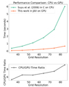 |
Fig. 1. Time comparison between CPU and GPU for extended image modeling of various source resolutions that arecommonly adopted in practice. The computation time is for a single iteration of a source and image intensity reconstruction given the values for lens mass model parameters. The computations took place on a 2.10 GHz CPU and an A100 GPU, respectively. |
3.1.2. Dark matter profile κenfw
We implement a dark matter profile following Oguri (2021) on the GPU, directly introducing ellipticity into the density mass profile κeNFW, in contrast to the classical approach, which incorporates ellipticity in the potential. Since all lensing properties of κeNFW have analytical expressions, computing κeNFW and αeNFW on a large grid of approximately 𝒪(103)×𝒪(103) takes a negligible amount of time, approximately 10−5 sec on a GPU. In contrast, performing the same computation on a CPU, following the approach of Golse & Kneib (2002), takes approximately 7 seconds. The detailed expressions for αeNFW and ψeNFW are provided in Appendix B.
3.2. GPU acceleration in dynamical modeling
As discussed in Sect. 2.4, the MGE is commonly used in dynamical modeling as a prerequisite for JAM. Without accounting for the internal MSD, the SB and mass density of the lens galaxies are sufficient for decomposition up to 3reff in dynamic modeling. When we considered the internal MSD, however, which represents a constant mass sheet added to the galaxy mass distribution, this additional mass can extend over a significantly larger region. To accurately account for the internal MSD, the mass profile must be decomposed over a larger area, approximately ∼50″ for lens system RXJ1131 (Yıldırım et al. 2023; Shajib et al. 2023).
In Yıldırım et al. (2023), the authors applied the 2D MGE fitting method (Cappellari 2002)5 to model the light and mass convergence map of the lens galaxy. In both cases, the maps are characterized by smooth profiles such as Sérsic, power-law, and NFW profiles, without any subtle angular structures. Since the maps primarily describe variations with radius, applying the 2D MGE fitting method is unnecessary in this case. The 2D MGE fitting method requires solving a non-linear least-squares minimization problem, which becomes computationally expensive when performed over a broad region extending ∼50″ from the lens galaxy center. Moreover, producing the light and mass convergence maps in 2D across a wide area with  pixels is rather time-consuming. In total, it takes 𝒪(10) s per sampling step. The MGE 2D fit is primarily used to capture more detailed structures in galaxies from optical imaging directly, rather than relying on maps derived from profiles.
We instead adopted the 1D MGE fitting method. We implemented a fast Gaussian decomposition to 1D profile following Shajib (2019) on GPU. In this approach, an integral transform with a Gaussian kernel is introduced:
 (40)
(40)
where F(z) represents any mass or light profiles that need to be decomposed using Gaussians. The transformed integral f(σ) can be approximated using the Euler algorithm:
 (41)
(41)
where ηn and χn can be complex-valued and are independent of f(σ). These values can be precomputed at the start. The standard deviations σn are chosen to be logarithmically spaced within the fitting region, resulting in:
 (42)
(42)
where the amplitude  , with wn representing fixed weighting factors and
  . This MGE approach fits each mass or light density profile using 21 Gaussians to recover the profile within ∼0.5% accuracy and runs in approximately 2 × 10⁻⁴ s on a single GPU.
We present the runtime of the 1D MGE fitting implemented in JAX in Table 2 and compare it with the NumPy version from Shajib (2019). In this case, GPU acceleration does not provide a significant speedup, achieving a runtime comparable to that of a single mass profile. Performance gains are realized when the models contain multiple 1D profiles of the same type, however. By leveraging the just-in-time (@jit) compiler and the vmap function in JAX, MGE fitting can be applied simultaneously to these profiles, improving efficiency. For readers interested in the speed comparison with the commonly used MgeFit package, we also provide a runtime comparison. In general, switching to the MGE 1D fit results in negligible computation time on both CPU and GPU.
Time comparison for one-step sampling in the joint modeling.
We reimplement part of the jam.axi.proj function from the JamPy package6 to compute  , the second velocity moment along the z′-axis on the plane of the sky. The main computational bottleneck lies in solving the Jeans equations (Eqs. (18) and (19)) to derive
  ,
,  , and
, and  (see Sect. 5.1 in Cappellari 2020). These computations involve numerical integrals, which are evaluated using adaptive quadrature methods in Shampine (2008). The integration region is initially divided into four subrectangles, and the integral in each subregion is computed using Gauss-Kronrod quadrature. If the estimated error in any subregion exceeds a predefined threshold, that subregion is further subdivided into four smaller subrectangles, and the process is repeated iteratively until the desired accuracy is achieved.
To enhance computational efficiency with the just-in-time (JIT) compiler, we modified the algorithm to use a fixed fine mesh. Specifically, the entire integration region is pre-divided into 64 subregions, with each subregion further subdivided into four smaller subrectangles, where Gauss-Kronrod quadrature is applied to compute the integral. The fractional error of  compared to the results from the JamPy package is, on average, 10−5, well within the relative error tolerance of 0.01 set by JamPy. This level of accuracy is sufficient given the relatively simple mass and light profiles used in this paper to compute
  . For more complex mass potentials and luminosity density tracers, however, a finer integration grid may be required to achieve the same level of precision.
Switching to the non-adaptive integral solver enables the simultaneous computation of  ,
,  , and
, and  at the required positions, significantly reducing the computation time from approximately ∼10 s to ∼0.3 s for over 200 points in polar coordinates on an A100 GPU, assuming a composite mass model. This model consists of baryonic and dark matter components, a BH, and a mass sheet to account for internal MSD (see Table 2).
3.3. Joint modeling
In this section we provide a detailed description of the joint modeling approach for time-delay cosmography. The input data dLD consist of both lensing and kinematic observations. The lensing data include the lens light, quasar image positions, the extended image of the host galaxy and the time delays between multiple observed images. The kinematic data comprise the spatially resolved kinematics map of the lens galaxy.
We use two Chameleon profiles to model the lens light in the optical image, which consists of two isothermal profiles with different core radii ωc and ωt,
 (43)
(43)
The goodness of the lens light fitting is evaluated by
 (44)
(44)
where Ij is the surface brightness in the pixel of the lens galaxy, and the PSF is the point spread function. The number of pixels Np used for lensing light modeling in Eq. (44) excludes those used for modeling extended arcs (which already account for the lens light).
We adopt parameterized mass profiles κint in the joint modeling. There are two mass classes.
-
κint, comp = (1 − λint)+λint(Υ* ⋅ Ilight + κenfw + κBH)
-
κint, epl = (1 − λint)+λintκepl.
In the first scenario, we model the baryonic component and dark matter of the lens galaxies separately. The baryonic component is represented by scaling the lens light profile Ilight, with a constant factor Υ*, while the dark matter is modeled using κenfw (see Eq. (B.1)). Ilight consists of two Chameleon profiles. The BH mass is included as a point mass κBH. In the second scenario, we use an elliptical power-law (EPL) profile κepl to represent the total mass (see Appendix C). Because the EPL profile has a softening scale rscale = 0.01″ that is set to a small value, the mass distribution diverges in the center, eliminating the need to add a separate point mass to represent the BH. In addition, we adopt an external shear to account for the tidal stretch from neighboring galaxies with external potential, expressed in polar coordinates (R, ϕ) as
 (45)
(45)
where γext represents the strength of the external shear, and the shear angle θext represents the stretching orientation of the images. We do not list the external shear in the above κint set-up because it adds zero contribution to the mass density with  .
.
In order to explicitly characterize the internal MSD, we adopt a dual pseudo-isothermal elliptical density (dPIE) profile (Elíasdóttir et al. 2007; Suyu & Halkola 2010), with a substantial core radius rcore = 45″ and truncated at rtr = 45.09″. This profile mimics a flat mass sheet up to a radius of ∼20″ before tapering down to zero. The extended arc observed at 1.65″ from the galaxy center implies that the lensing-only modeling remains unaffected by this additional mass sheet, rendering the distance DΔt,int completely degenerate with λint (Yıldırım et al. 2023). The expression for λint is:
 (46)
(46)
where a0 is a normalization parameter and R2 = x2 + y2. In the region where R ≪ rcore, we obtain an approximately constant mass sheet
 (47)
(47)
In the region where R ≫ rtr, we have λint ≃ 1, indicating that the added mass sheet effectively vanishes at large scales. We emphasize that the values of rcore and rtr are carefully selected based on extensive testing to represent the worst-case scenario. While the internal MSD remains unaffected from a lensing perspective, its impact on the kinematic data are significant enough to impose constraints on λint. In addition, the dPIE profile, which features a well-defined truncation radius, declines more rapidly than the mass-sheet profile used in Blum et al. (2020). This makes it a more suitable choice, as it helps reduce the likelihood of having negative values for κint in the outermost regions. Negative mass convergence is unphysical and is therefore rejected by JAM.
Ideally, a mass profile for λint that characterizes the internal MSD for lens system RXJ1131 would remain constant out to ∼20″, and then drop sharply to zero beyond that radius. This behavior would entirely prevent the emergence of negative κint. An ideal mass sheet like this, however, lacks well-defined lensing properties and is difficult to fit using the MGE. We adopted a dPIE profile with a fixed rcore to represent the mass sheet. The relatively gradual decline of the dPIE profile in the outermost region and the fixed rcore can lead to negative κint, resulting in an asymmetric probability distribution for DΔt, int (see Sect. 5.2).
Using the chosen mass density model, either a composite or power-law model, along with Ilight, we perform lensing and dynamical modeling simultaneously (see Fig. 2). Both the light and mass density profile of the lens galaxy must have the same position angle φPA, to maintain the axisymmetric assumption. In our joint modeling, we fix this position angle to the mock input value. On the lensing side, we model the extended arc, lensing light, image positions, and time delays. For dynamical modeling, we decompose Ilight and Σint into multiple Gaussian components. The MGE is carried out up to 50″ from the lensing centroid, corresponding to approximately 200 kpc, ensuring that the mass density κint, transformed by the internal mass sheet, remains physically meaningful at large distances. We restrict our analysis to models with strictly positive total mass density, as negative values would yield unphysical predictions for  . The predicted kinematic map is then computed by feeding the MGEs of Ilight and Σint into the JAM framework (see Sect. 2.4). In practice, the light Ilight, IFU near the spectral absorption lines in the IFU data should be provided to JAM to trace the stellar population responsible for these lines. In this paper, we work on the simulated kinematic data. We instead use the best-fit lens light model from the F814W filter in the infrared band. Since the lens galaxy in RXJ1131 is an early-type elliptical galaxy, the infrared band effectively characterizes the dominant stellar populations.
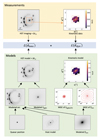 |
Fig. 2. Workflow for the joint modeling using RXJ 1131 as an example. The input datasets consisted of photometric images and the spatial kinematics of the lens galaxy. The red contours in the middle right of the green panel represent the isocontours of both the light and mass density distributions of the lens galaxy, derived from the MGE method (see Sect. 3.2). The modeled Ilight represents the light fitted from optical imaging, and Ilight, IFU corresponds to the light near the spectral absorption lines in the IFU data. In the paper, Ilight is equivalent to Ilight, IFU. We employed an MCMC sampler to simultaneously sample the parameter space ηLD for the lensing and the dynamical modeling. |
The best-fit model is determined through joint modeling within a Bayesian framework. We sample the posterior distribution of parameters  (see Eq. (48)) using the Metropolis-Hastings Markov Chain Monte Carlo (MCMC) method,
 (48)
(48)
where dL presents the lensing data, dD the kinematic data, and P(ηLD) the prior for the lensing and dynamical parameters. The goodness-of-fit for a model is defined as
 (49)
(49)
The MCMC sampling is conducted on the CPU, where ηLD, involving approximately 10 parameters, is drawn and then transferred to the GPU for extended image, lens light and dynamical modeling. Since the image-position and time-delay modeling involves processing a relatively small dataset, it is kept on the CPU. Although data transfer between the CPU and GPU incurs some latency, the number of transferred data points in our case is on the order of ∼𝒪(10), resulting in a negligible transfer time.
We achieve a 20× speedup per sampling step using JAX on a single A100 GPU. Table 2 presents the runtime for each step using a composite mass model. Additionally, we include the runtime of the JAX code on a CPU for readers interested in evaluating the parallelization performance gains of JAX on different hardware. We note that JAX is primarily optimized for GPU. On CPUs, its compilation overhead, lack of CPU-specific optimizations, and execution graph transformations can make it slower than NumPy.
3.4. Bayesian information criterion
In this section we introduce a BIC method to distinguish the goodness of the mass models of the lens galaxies with different ηLD. The BIC is an approximation to the Bayesian evidence,
 (50)
(50)
where ℳ is the constructed mass model with parameters ηLD. The BIC is defined as
 (51)
(51)
where k is the number of parameters in the model, n is the number of data points, and ℒ is the maximum likelihood of the model. The BIC penalizes models with a higher number of parameters, effectively balancing goodness of fit with model simplicity. The likelihood in our case is the product of the lensing modeling ℒ(dL | ηLD) and dynamical modeling ℒ(dD | ηLD). The likelihood is easily overwhelmed by the lensing data due to the large number of pixels on the extended arcs. We focused on using spatially resolved kinematics data to break the internal MSD and constrain λint. The lensing-only modeling cannot constrain λint or distinguish between a composite and an elliptical power-law model. Therefore, we exclude ℒ(dL | ηLD) and the lensing data points, relying on ℒ(dD | ηLD), the number of kinematic data points, and the number of parameters ηLD adopted in the joint modeling to weight the posterior distribution.
We identify ℳmin as the model with the lowest BICmin, which corresponds to the minimal χdyn2 from the dynamical modeling (since k and n remain the same). The probability ratio of a model ℳi to the model ℳmin given the data dLD is
 (52)
(52)
After normalizing for Nm models, we obtain the weighting factor for each model ℳi,
 (53)
(53)
with BICi − BICmin > = 0. As discussed in Sect. 3.1, the preferred lensing mass parameters vary across different parameter spaces depending on the source resolution. The choice of source pixelization introduces uncertainties in the BIC for a given lens mass parametrization (see Appendix D). To quantify this uncertainty, we compare the BIC values across different source grids and measure the root-mean-square scatter σBIC. Following Birrer et al. (2019) and Yıldırım et al. (2020), we incorporate this uncertainty into the model weighting by convolving fBIC in Eq. (52) with a Gaussian distribution of variance σBIC2, thereby obtaining the updated model weights:
 (54)
(54)
where
 (55)
(55)
4. Simulated mock datasets
The lens galaxiy RXJ1131 was discovered by Sluse et al. (2003). It is located at a redshift of zlens = 0.295, while the lensed source galaxy is at a redshift of zs = 0.654, both confirmed through spectroscopy (e.g., Sluse et al. 2007). The lens is accompanied by a faint satellite galaxy S (see Fig. 3), which JWST NIRSpec has confirmed to be at the same redshift as the lens (see Shajib et al. (2025)). Imaging data were collected from the Hubble Space Telescope (HST) Advanced Camera for Surveys (ACS) with an exposure time of 1980 seconds. Time-delay measurements for RXJ1131 were made through a dedicated optical monitoring campaign under the COSMOGRAIL program (e.g., Tewes et al. 2013). These measurements, based on frequent observations (every 3 days) over more than 9 years and involving over 700 epochs using meter-class telescopes and new curve-shifting techniques, reported an approximately 3% precision time delay by Tewes et al. (2013), Liao et al. (2015), Bonvin et al. (2017). Microlensing-induced time-delay shifts, as analyzed by Tie & Kochanek (2018), have been found to be negligible within the context of the extended delay, as discussed by Chen et al. (2018).
 |
Fig. 3. Mock data sets of the lensing imaging and kinematic data. We observed a faint satellite galaxy above the lens galaxy at the same redshift as the lens galaxy. We neglected the satellite when we simulated the IFU data. The satellite is too small to extract useful kinematic information from the IFU datacube other than the redshift (see Shajib et al. 2025). More importantly, based on the previous study, the satellite has a negligible effect on mass modeling and cosmological distance inference (Suyu et al. 2014). The mock IFU data with 52 bins are presented in the same reference frame as the simulated HST imaging. North is up, and east is to the left. |
To generate the mock HST imaging of RXJ1131, we use the best-fit mass model obtained from lensing-only modeling of the HST F814W-band imaging, with a source grid resolution of 64 × 64. The mass model consists of a composite profile, where the baryonic component is represented by two Chameleon profiles (see Eq. (43)) scaled by a constant and the dark matter halo is characterized by κenfw. Additionally, the model includes an external shear and a fixed BH mass. The lens galaxy in RXJ1131 exhibits a high central velocity dispersion σdisp with σdisp = 320 ± 20 km s−1 (Suyu et al. 2014; Shajib et al. 2023). By applying the scaling relation between σdisp and MBH (e.g., Kormendy & Ho 2013; McConnell & Ma 2013), we estimate the BH mass to be between 109 M⊙ and 1010 M⊙. Kormendy (2013) predicts MBH ≈ 2.4 × 10⁹ M⊙, while the version by McConnell & Ma (2013) gives MBH ≈ 3.0 × 10⁹ M⊙. We set a higher BH mass of MBH = 5 × 10⁹ M⊙ in the simulated kinematic data to explore its effects in cosmography inference. This value remains a reasonable estimate, as suggested by Fig. 16 of Kormendy & Ho (2013) and Fig. 1 of McConnell & Ma (2013). We do not add any mass sheet to the best-fit model, ensuring that  , indicating no MSD in the simulated data. We randomly select an external convergence value of
  as the ground truth based on the probability distribution function obtained from ray tracing through the Millennium Simulation for the composite mass model (e.g., Suyu et al. 2014).
To simulate the kinematics map, we follow the approach presented in Yıldırım et al. (2020). We use the best-fit lensing light map for the kinematic mock data and assume a Poisson noise-dominated region. The relative pixel intensities are then converted into a relative 2D signal-to-noise map. We adopt VorBin7 package (Cappellari & Copin 2003) to apply the adaptive spatial binning to the signal-to-noise ratio map, with a target signal-to-noise ratio of 50 per bin. We simulate the data with a high signal-to-noise ratio to ensure that by combining high-quality kinematic data, the internal MSD can be effectively broken. Considering the light contamination from nearby quasar images and the extended host galaxy at the Einstein radius of θE ≃ 1.65 ″, the simulated binned map covers a small field of view (FoV) ranging from −1″ to 1″ relative to the lens centroid (see Fig. 3). For simplicity, we neglect the satellite when mocking up the IFU map as well as during the modeling of the SL and stellar kinematic data. We assume a single Gaussian kinematic PSFkin with a FWHM of 0.14″, which corresponds approximately to the PSF measured from JWST NIRSpec data of RXJ1131 (see Shajib et al. 2025). We generate the noiseless kinematic map with JamPy8 package based on the mass and light distribution from the best-fit lens model (refer to the best-fit parameters in Table 3) and the simulated binned map.
Model parameters and prior for the joint modeling.
We simulate two kinematic datasets. The first is an ideal kinematic dataset where only statistical errors are added to the noiseless kinematic map:
 (56)
(56)
where δvstat,l = Gaussian[0, 0.02vrms,l]. We assume a statistical error of approximately 2% of the bin values for each Voronoi bin l. In the second kinematic dataset, we introduce a 5% systematic bias to test the impact of potential misfits in the kinematic data:
 (57)
(57)
Systematic errors can arise during the kinematics extraction process, as the measured kinematics may be biased by different methods, such as stellar population synthesis and the use of various stellar libraries such as X-Shooter (Verro et al. 2022a,b), MILES (Vazdekis et al. 2016), and Indo-US (Valdes et al. 2004). By carefully cleaning the stellar libraries before measuring the kinematics, however, these systematic errors can be controlled to within the subpercent level (see Knabel et al. 2025). We tested an overly high level of systematics of 5% in order to illustrate the impact of a systematic shift in kinematics on the distance inference, even though we anticipate sub-percent level kinematic shifts in reality.
5. Analysis and discussion of the joint modeling results
In this section we present the results of the joint modeling using mock lensing and kinematic data. In Sect. 5.1, we outline the joint modeling setup and describe the modeling procedure. In Sect. 5.2, we discuss the fitting results of the joint modeling and demonstrate how it breaks the internal MSD, given ideal kinematic data. In Sect. 5.3, we analyze the effect of systematic errors in the kinematic map on H0, given the 5% biased kinematic data. In Sect. 5.4, we examine the impact of MBH on H0 inference, given ideal kinematic data. In Sect. 5.5, we present joint modeling based on ideal kinematic data, excluding the central region, to test whether the impact of an unknown black hole mass can be mitigated, thereby reducing potential bias in distance measurements. We also discuss how the MBH–βani degeneracy has been addressed in the literature and explore the potential for applying these solutions to lensing and dynamical modeling.
5.1. Joint modeling setup and procedure
The mass models adopted in our joint modeling are κint, comp and κint, epl (see Sect. 3.3). Both explicitly represent the mass sheet using a dPIE profile. In the composite model, each component of the galaxy is modeled separately with distinct mass profiles. To account for the central BH, we consider the lens galaxy in RXJ1131, whose velocity dispersion has been measured as σdisp = 320 ± 20 km s−1 by Suyu et al. (2014). Using the MBH − σdisp relation, we explore the full range of possible BH masses of [109 M⊙,1010 M⊙] to be conservative. For each composite mass model setup, we fix the BH mass and increment it in steps of 109 M⊙ across the specified range. In contrast, the EPL mass model treats the galaxy as a single mass component and does not include an additional mass profile for the BH.
For each mass model setup, whether using κint, comp or κint, epl, we perform joint modeling across a range of source grids, from 60 × 60 to 68 × 68 pixels, increasing in steps of 2. This variation accounts for potential degeneracies introduced by the source-grid resolution. These resolutions are sufficient to mitigate parameter degeneracies while ensuring a good fit to the extended arcs (see Appendix D for details).
The lensing constraints in the joint modeling are consistently provided by the same simulated lensing data. For the kinematic input, we consider two sets of simulated data: one ideal (see Eq. (56)) and one with a 5% bias (see Eq. (57)). For each case, we perform 55 joint modeling runs (1 EPL model plus 10 composite models for the 10 fixed BH masses, and each of the 11 models has 5 source-grid resolutions). The final posterior distributions of the lensing and dynamical parameters are then obtained by combining the results of these 55 models using BIC weighting (see Sect. 3.4), for the ideal and 5% biased kinematic datasets, respectively.
5.2. Breaking the MSD using joint modeling
In this section we illustrate how joint modeling resolves the internal MSD given an ideal kinematic dataset. The time-delay distance DΔt, int is entirely degenerate with λint over the prior range of λint when considering lensing-only modeling. The kinematic data aid in constraining λint and in identifying the uniquely preferred κint model within the range λint ∈ [0.5, 1.5]. Consequently, we can break the internal MSD and firmly constrain DΔt,int (see the red box in Fig. 4).
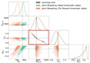 |
Fig. 4. Measurements from the joint modeling (combining all mass models) and lensing-only modeling. The shaded contours represent 1σ, 2σ, and 3σ confidence regions. The green contours correspond to the joint modeling using the ideal kinematic data, and the orange contours correspond to the joint modeling using kinematic data with a 5% systematic bias. The gray contours represent the lensing-only modeling. The red box indicates the degeneracy between DΔt, int and λint in the lensing-only modeling. |
We present both equal-weighted and BIC-weighted histograms of Dd and DΔt, int in Fig. 5. The BIC does not clearly distinguish between composite mass models with BH masses in the range MBH = 2 × 10⁹ M⊙ to 5 × 10⁹ M⊙, as the differences in BIC values ΔBIC are comparable to their associated uncertainties σBIC (see Appendix F). Outside this mass range, as well as for the EPL model, the BIC is more effective at discriminating between models. The limited effectiveness of BIC weighting is consistent with expectations, as MBH cannot be well constrained by dynamical modeling for galaxies beyond the local Universe. The EPL model, in particular, exhibits higher scatter in the probability density distribution of DΔt, int across different source resolutions. This increased scatter is likely due to the fact that the mock kinematic data were generated using a composite mass model. Since the EPL model assumes a single power-law mass profile, it fails to fully capture the complexity of the true lens mass distribution, leading to less reliable constraints on DΔt, int. Despite this internal scatter, the EPL model is statistically disfavored under BIC weighting. It consistently underperforms in fitting the mock kinematic data. We obtain a minimal discrepancy of  of the EPL model across different source grid resolutions relative to the best-fit composite mass model (see Fig. 6).
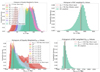 |
Fig. 5. Top panels: Marginalized posterior density distribution of Dd, based on the joint models using ideal kinematic data. The different colors represent posterior densities corresponding to different BH masses, while each color represents five separate posterior distributions that are tightly clustered together, corresponding to models with identical mass parameterizations but different source-grid resolutions. The red color represents EPL mass models, where a small softening scale of rsoft = 0.01″ mimics the presence of a massive BH, eliminating the need to explicitly include an additional MBH. The left panel shows equally weighted Dd posterior densities, whereas the right panel presents the combined Dd posterior density weighted by BIC (see Sect. 3.4). Bottom panels: Marginalized posterior density distribution of DΔt, int, based on joint models using ideal kinematic data. The red dashed lines in both panels indicate the mock input values used in the simulated data. The black dashed lines represent the median values in the BIC-weighted distribution. |
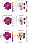 |
Fig. 6. Best-fit kinematic maps from the joint models for different BH mass assumptions. The displayed kinematic bin maps have 52 bins in total. Upper Panel: Joint modeling is performed using a grid of MBH values ranging from 109 to 1010 M⊙. In each model, the BH mass is fixed and incremented in steps of 109 M⊙ within this range. The best-fit kinematic map, corresponding to MBH = 3 × 10⁹ M⊙, achieves χdyn2 = 50. Middle Panel: The best-fit kinematic map from joint modeling that assumes no BH, yielding χdyn2 = 64. Lower Panel: The best-fit kinematic map from joint modeling using the EPL mass profile, resulting in χdyn2 = 58. |
We combine all 55 models, obtaining the recovered time-delay distance  Mpc, which deviates from the mock input by 1.87%, within the 1-sigma uncertainty range. Similarly, the recovered lens distance
  Mpc shows a deviation of 0.77%.
The uncertainty in DΔt, int is asymmetric, exhibiting a longer tail on the positive side and a shorter tail on the negative side (see Figs. 4 and 5). This occurs because, as λint approaches the upper bound of 1.5 in the prior, it implies that κgal is being modified by the addition of a negative constant sheet (1 − λint) on top of λintκgal (see Eq. (6)). In regions far from the lensing centroid, κint becomes negative, which is not allowed under the dynamical modeling framework of JAM. As a result, the probability distribution of DΔt, int becomes asymmetric (see Sect. 3.3). The lower 1σ bound of 78 Mpc may be underestimated relative to the true 1σ interval, assuming that λint follows an “ideal” mass sheet profile with a sharp cutoff beyond ∼20″, which mimics the MST and also allows higher values of λint without leading to negative κint. The probability distribution of Dd is also slightly asymmetric, but it is less pronounced than that of DΔt,int. The asymmetry in Dd arises from the influence of MBH, which is discussed in more detail in Sect. 5.4.
With the posterior probability distribution P(DΔt, int, Dd ∣ dLD), we infer H0 and Ωm in a flat Λ CDM universe. We adopt uniform priors on H0 between [50, 120] km s−1 Mpc−1 and on the matter density parameter9Ωm between [0.05, 0.5]. We generate 5 × 10⁵ samples for the parameters {H0, Ωm} and calculate the corresponding DΔt,int10 and Dd values using the lens and source redshifts under a flat ΛCDM cosmology. For each sample, we randomly draw a κext value from the external convergence distribution inferred by Suyu et al. (2014) and scale the distance using Eq. (12) to obtain DΔt, int. Subsequently, we weight the samples using P(DΔt, int, Dd ∣ dLD). From the weighted sample distribution, we obtain constraints on  (see Tab. 4). We also present H0 values derived from the posterior probability distribution, marginalized over all parameters, including DΔt,int and Dd separately. The value
  , obtained from P(DΔt, int), reflects asymmetrical uncertainties inherited from DΔt,int distribution. These skewed uncertainties of the inferred H0 are mitigated by incorporating both distances
  , however (see Table 4 and Fig. 7). This demonstrates the advantage of joint modeling, where using two distances improves the constraint on H0. The value of Ωm inferred by joint modeling is poorly constrained from a single lens system; therefore, it is not included in the table.
Inferred H0 and key parameters for the models.
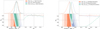 |
Fig. 7. H0 and Ωm constraints from our models in a flat |

5.3. Impact of a high systematic bias in the kinematics data on the H0 measurement
In this section we perform joint modeling of the kinematic data, incorporating a 5% systematic bias (see Eq. (57)) to account for measurement-related systematic errors in the kinematic map. We emphasize that this adopted error represents a worst-case scenario, in which the kinematic measurements are not optimally performed. Furthermore, we highlight the importance of achieving sub-percent systematic errors in the kinematic map to ensure the robustness of cosmographic modeling, using the method presented in Knabel et al. (2025).
The 5% biased kinematic data also help break the internal MSD, yielding consistent results for  and
and  Mpc, which agree with values inferred from the joint modeling using ideal kinematic data. This demonstrates that the overall systematic bias does not affect the constraints on DΔt, int and λint (see Fig. 4). This is because λint is constrained by the 2D kinematic map, where the shape of the vrms profile breaks the internal MSD and constrains DΔt, int. The 5% bias does not alter the shape of the vrms profile, which is why neither DΔt, int nor λint is biased. The orbital anisotropy parameter, βani, is primarily constrained by the shape of the kinematic map; therefore, its inference remains robust. We obtain
  , which is consistent with the value inferred from the ideal kinematic data.
The systematic bias primarily impacts Dd because it changes the amplitude of the vrms overall. Given the relation  , a 5% bias in
  results in an expected ∼9% bias in Dd. We obtain
  Mpc, which is 9% lower than the mock input value of Dd = 775 Mpc, as expected. If the combined kinematics are obtained from a single aperture rather than an IFU, the impact on distances will not be cleanly isolated to Dd alone, as the single aperture lacks information on the shape of vrms. We anticipate a more severe effect on both Dd and DΔt, int.
The inferred value of  from P(Dd) is biased by 13% compared to the mock input. Because the inferred DΔt, int remained unbiased, however, we obtained
  using P(DΔt, int, Dd ∣ dLD), which carries a bias of 6% relative to the mock input (see Fig. 4).
Any systematic error affecting the overall kinematic map will be amplified in Dd inference (Chen et al. 2021). Although the bias does not impact DΔt, int inference, the joint modeling of H0 remains highly susceptible to bias. This crucially highlights the importance of accurately measuring kinematics and controlling systematic uncertainties to the sub-percent level, which is achieved by Knabel et al. (2025), in order to measure Dd and H0 to the percent level.
5.4. Impact of the MBH − βani degeneracy on the H0 measurement in time-delay cosmography
The BH in lensing-only modeling is often neglected since SL only provides constraints at Einstein radius, which is far from the galaxy’s center. Only in some rare cases, the lensed source image appears close to the galaxy center within ≲1 kpc (e.g., Nightingale et al. 2023; Melo-Carneiro et al. 2025). Kinematic data can provide some constraints, but its effectiveness is highly limited by the instrument’s resolution, particularly for galaxies at galaxies at z > 0.1. The lens galaxy RXJ1131 at z = 0.295 might hold a supermassive BH with MBH in the range of [109, 1010] M⊙ which corresponding to a sphere of influence rsoi for the BH in the range of [0.011″, 0.11″]. The simulated kinematic data have a spaxel size with 0.1″ convolved with  of
of  . For MBH near 1010 M⊙, the influence of the BH dynamics can be imprinted on the central Voronoi bins.
We investigate the impact of the BH on distance inference using joint modeling with ideal kinematic data. This is due to the well-known mass–anisotropy degeneracy (e.g., Binney & Mamon 1982; Treu & Koopmans 2002; Courteau et al. 2014) in spherical systems, where a wide range of density profiles can be matched by varying βani while keeping the observed vrms unchanged. The lens galaxy in RXJ1131, as a slow rotator with a nearly spherical central structure, is affected by this degeneracy (Cappellari 2016).
The joint modeling results show that the inferred values of βani span the full prior range of [−0.3, 0.3] (see Fig. 8), given a black hole mass in the range MBH ∈ [109, 1010] M⊙. This prior range is motivated by studies of nearby massive elliptical galaxies (see review in Cappellari 2025, Figs. 8, 10), and is quite conservative in its broad range compared to the typical scatter of anisotropies of galaxies shown in Cappellari (2025). The anisotropy βani is constrained by the spatial pattern in the kinematic data. MBH and βani similarly affect the stellar motions in the galaxy centroid, however, resulting in a trade-off between them. In Fig. 8, we observe that a heavier MBH leads to a smaller βani, and vice versa. A higher MBH deepens the central gravitational potential, allowing more tangential orbits in the dynamical model when reproducing the same observed line-of-sight velocity dispersion, corresponding to βani < 0. Conversely, a lower MBH can produce similar velocity dispersions if the stellar orbits are more radial, with βani > 0, as radial orbits allow stars to reach higher line-of-sight velocity dispersion near the galaxy center. Both BH mass and βani contribute to accelerating stellar motion, but in different directions.
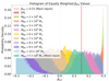 |
Fig. 8. Marginalized posterior density distribution of βani based on the joint models using ideal kinematic data. Different colors represent posterior densities corresponding to different BH masses, while the same color indicates models with identical mass parameterization but different source grid resolutions. We observe that as MBH increases, the inferred βani decreases and vice versa. The inferred βani distributions given different MBH spread over the prior range [−0.3,0.3], but different MBH yield different goodness of fit to the kinematic data (as shown in Fig. 5). |
A trade-off between MBH and βani can lead to a misestimated βani, which in turn affects the accuracy of the distance inference, particularly in Dd. When the BH mass used in the modeling is lower than the mock input value, a higher value of βani is required to fit the kinematic data. Since we assume a constant βani across all radii in the joint modeling, this means that even in the outer regions where  adjustments are unnecessary,
  are still affected by βani. To match the observed kinematics beyond the central region, Dd increases to counterbalance the effect introduced by changes in βani. This is because Dd acts as a normalization factor for scaling
  , following the relation
  (see Sect. 2.4). If the BH mass in the joint modeling is heavier than the mock input, the entire trend reverses. This explains the observed correlations in the values of Dd, βani and MBH (see Figs. 5, 8 and 9). In Fig. 9, we observe a negative correlation between the adopted MBH in the joint modeling and Dd. BH masses in the range of MBH = 2 × 10⁹ M⊙ to MBH = 7 × 10⁹ M⊙ are difficult to distinguish based on kinematic data and all contribute to the inference of distances in the BIC framework, given the MBH = 5 × 10⁹ M⊙ in the mock input. This results in a slight asymmetry in the probability distribution of Dd. Since we use P(dD ∣ ℳi) for BIC weighting in the joint models, some models with lower or larger BH masses can still provide comparably good fits to the kinematic data as the model with the true MBH, by appropriately rescaling both Dd and βani. These models contribute to the extended tails of the inferred Dd distribution (see the upper panels in Fig. 5). Nonetheless, the inferred Dd recovers the mock input value within the 1σ uncertainty. For the same underlying reason–but with a more pronounced impact–the constraint on βani is significantly weaker. As a result, βani is not tightly constrained, with an inferred value of
  (see Tab. 4).
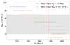 |
Fig. 9. MBH vs. Dd with 1σ uncertainties based on the ideal kinematic data. This provides a clearer visualization of the upper-left panel in Fig. 5. The plot also illustrates how the BH mass affects the inference of Dd, given that βani is within the prior range of −0.3 to 0.3. The gray shaded region represents models with the BH mass satisfying |

While the above analysis considers a range of plausible BH masses with BIC weighting, we now turn to the case of a single, incorrect BH mass assumption to examine its impact on the inferred distances. First, we test the scenario where we assume no BH in the composite mass model. The inferred value of  successfully recovers the input H0 value (see Fig. 10 and Table 4). The best-fit kinematic map exhibits a significantly different pattern than the one obtained when the BH is included in the modeling, however (see Fig. 6). The difference of Δχdyn2 = 14 for the dynamical fit indicates a poorer fit compared to the best-fit model that accounts for the BH. The fitted value of
  reaches the upper bound of the prior range, yet it remains insufficient to fully compensate for the absence of the BH, leading to a suboptimal fit to the kinematic data. The high βani value leads to an excessive increase in velocity dispersions in the outer regions. As a result, this imbalance starts to affect the probability density distribution of DΔt, int. To compensate for the effect induced by βani, DΔt, int decreases slightly.
A possible explanation is that the high βani requires a significantly different mass model than initially assumed to fit the kinematic data, which in turn affects λint and DΔt, int. We obtain a lower value of  Mpc, with a median value that is 3% lower than the input value. The reason H0 can still be recovered in this case is that Dd is recovered to within 1% of its input value. When the prior range of βani is extended beyond 0.3, however, its inferred value continues to increase until it adequately fits the kinematic data. As a result, Dd increases accordingly to counterbalance the effect of βani in the outer regions. This will ultimately introduce additional bias in Dd that exceeds the value reported in Table 4, thereby biasing the inferred H0 value.
In the second case, we probe the scenario where an incorrect BH mass of MBH = 7 × 10⁹ M⊙ was assumed. In contrast to the first case, the orbital anisotropy  shifts toward the lower bound, and the value of
  Mpc is lower than the Dd obtained using the true MBH = 5 × 10⁹ (see Fig. 9). In this case, the best-fit kinematic map can reach almost the same quality as the model that uses the true BH mass. The value of Dd is lower, however, and the inferred value of
  therefore is 3% higher than the mock input value of
  (see Fig. 10).
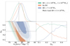 |
Fig. 10. Constraints on H0 and Ωm from our models in a flat |

The above tests indicate that a severely misfitted βani can strongly bias Dd and mildly influence DΔt, int in the extreme case, thereby affecting H0 inference, even when the kinematic data appear to be well-fitted. The value of βani can be accurately recovered when the BH mass is known and vice versa. We find that the fitted value of  is well constrained when the true MBH is used in the joint modeling (see Table 4). In nearly all cases of lens galaxies, however, the precise BH mass is unknown. The bias in Dd caused by a misfitted βani can be mitigated by performing joint modeling over a range of possible BH masses and using the BIC to downweight models that are disfavored by the kinematic data. It naturally follows that the prior range of βani should be carefully chosen Simon et al. (2024). Expanding the prior range allows adjustments to βani and Dd to always effectively compensate for the presence of the BH. While this results in a well-fitted kinematic model, it significantly biases the inferred Dd.
5.5. Mitigating the impact of the MBH–βani degeneracy on the H0 measurements
We set the BH mass in our simulated datasets to MBH = 5 × 10⁹ M⊙, corresponding to a sphere of influence radius of rsoi = 0.056″. As a result, the BH primarily affects the inner region. To account for this, we exclude the nine central bins in the ideal simulated kinematic map within the FoV range of  to
to  . We then examine whether the joint modeling becomes insensitive to the BH mass, thereby mitigating the bias in the
  measurement caused by the MBH–βani degeneracy.
We perform joint modeling using the ideal kinematic map while excluding the central regions. We reassess the recovery of the H0 value and evaluate the quality of the kinematic fit for both cases of no BH and a BH with  . In both cases, we observe that Dd and βani shifted closer to the mock input values, allowing for an accurate recovery of H0 within 1σ uncertainties (see Table 4 and more details in Appendix E). As anticipated, the 1σ uncertainties are broader than the full ideal kinematic dataset because we adopt 43 bins instead of the complete dataset with 52 bins. Additionally, the kinematic data excluding the central region is effectively recovered through joint modeling with no BH and
  (see Fig. 11). This suggests that excluding the central kinematic region can help mitigate the impact of a BH with a highly uncertain mass, and reduce potential biases in distance inference. In both cases, however, βani remains poorly constrained. This is due to the fact that the outer regions of galaxies are often significantly influenced by dark matter. The presence of dark matter introduces its own mass–anisotropy degeneracy, which complicates the interpretation of kinematic data in these regions–similar to the effect of the BH in the central regions. As a result, determining βani using only the outer kinematic bins is challenging due to the unknown distribution of dark matter.
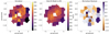 |
Fig. 11. Left: Ideal kinematic data without the bins within −0.15″ to 0.15″ with 43 bins in total. Middle: Best-fit kinematic map with |


To fully resolve the MBH–βani degeneracy, one effective way is to use the full line-of-sight velocity distribution (LOSVD). Instead of relying only on vrms, incorporating higher-order moments like h3 and h4 provides stronger constraints on the orbital structure. This approach, however, demands high signal-to-noise data and advanced modeling techniques, such as Schwarzschild’s orbit-superposition method (Cappellari et al. 2009; Thomas et al. 2014, 2016; Poci & Smith 2022). The lens galaxy of RXJ1131 at z = 0.295 even with JWST NIRSpec data are unlikely to reach the required resolution and signal-to-noise ratio to perform such modeling.
Another approach, while still relying only on vrms in JAM modeling, is to adopt a physically motivated prior for a more flexible orbital anisotropy. This can be informed by studies of well-observed nearby galaxies, as demonstrated in Simon et al. (2024). In that work, the author introduced a radially varying anisotropy profile, βani(r), and carefully defined the prior range based on physical expectations. Specifically, the central regions near the black hole are assumed to be more tangentially biased, while the outer regions are expected to be more radially anisotropic. This pattern is supported by theoretical predictions that dry mergers eject stars on radial orbits, which pass close to a central supermassive black hole binary. Such interactions can create a core in the surface brightness profile and lead to a dominance of tangential orbits in the central region, while the stars in the outer regions retain a more radial orbital distribution. This scenario is consistent with both observations and simulations (e.g. Milosavljević & Merritt 2001; Rantala et al. 2018; Saglia et al. 2024).
In principle, a similar method, incorporating well-justified anisotropy priors, could also be useful in lensing-based dynamical analyses. The current version of our modeling code only supports a constant anisotropy for the radii, however. Fully resolving the MBH–βani degeneracy is beyond the scope of this paper. Instead, the main goal of this work is to show that, once this degeneracy is reasonably mitigated, it does not introduce significant bias on the inferred cosmological distances.
6. Summary and outlook
We presented a GPU-accelerated code (GLaD) for a self-consistent lensing and dynamical modeling that is based on Yıldırım et al. (2020) for the lensing part and on Cappellari (2020) for the dynamics part. This method combines lensing and dynamical models by solving the Jeans equations in an axisymmetric geometry. The primary purpose of this code is time-delay cosmography, but it can also be applied to galaxy evolution studies (Shajib et al. 2021; Tan et al. 2024; Sheu et al. 2025; Sahu et al. 2024).
In time-delay cosmography, it is essential to account for parameter uncertainties. The most time-consuming part of the joint modeling is running analyses on a range of source grids to account for the parameter uncertainties that are associated with the source grid resolutions. Another computational challenge is solving the Jeans equation to determine the intrinsic second velocity moments. The first issue is optimized using GPU architecture, which excels at accelerating large matrix calculations, while the second is handled with a nonadaptive integral solver. In both cases, we achieved a speed-up of at least an order-of-magnitude.
We simulated the lensing and kinematic data for the lensed quasar system RXJ1131 to test whether GLaD can recover the mock input value. The central velocity dispersion of the lens galaxy in RXJ1131 is ≥300 km s−1, and we therefore added an MBH = 5 × 10⁹ M⊙ in the mock mass profile. For the kinematic map, we generated one ideal kinematic map with a statistical error of 2% and a biased kinematic map with a systematic bias of 5% (as a worst-case scenario) in all the velocities. We used GLaD to perform the joint modeling on the simulated data to test the effect of the systematic error and BH effects on the kinematic map. Our results are listed below.
-
GLaD achieved a sampling time of ∼0.5 seconds per step on a single A100 GPU. This reduced the Bayesian inference of the joint modeling in Yıldırım et al. (2020, 2023) from a month to several days.
-
We performed the joint modeling using two types of mass models and combined 55 models based on the BIC weighing. As expected, the kinematic data helped us to break the internal MSD. With ideal kinematic data, we achieved an uncertainty of 4% on the inference of H0.
-
Systematic biases in the overall amplitude of spatially resolved kinematic data do not significantly impact the constraints on λint and DΔt, int because these parameters are primarily sensitive to the shape of the two-dimensional vrms distribution. Since an overall bias only alters the amplitude and not the shape of vrms, its effect on the inference of these parameters is very weak.
-
The bias in the amplitude of vrms primarily affects the inference of Dd. A bias of 5% leads to a bias of approximately 10% in Dd, which in turn results in a bias of 10% on the H0 measurement, given P(Dd). As we emphasized earlier, however, a bias of 5% in the kinematic data do not bias DΔt, int. Consequently, when H0 is considered with both distances, P(Dd, DΔt, int), the bias is reduced to approximately 6%. We demonstrated that the systematic bias in the kinematic data double the error as it propagates to H0 (as also shown by Chen et al. 2021, see Eqs. 20 and 21). This highlights the importance of measuring the kinematics with a subpercent systematic uncertainty, as was recently achieved by Knabel et al. (2025).
-
The BH mass does not affect the breaking of the internal MSD. The measurement of
 and
and  therefore remains independent of the adopted MBH in the joint modeling, provided that the kinematic data are well fit.
 -
Given the high BH mass of 5 × 10⁹ M⊙ we adopted in our mock data, the BH mass plays a crucial role in constraining βani and Dd. By adjusting βani, we can mimic the effect of a massive BH, which makes it difficult to constrain the anisotropy without a precise knowledge of the BH mass. Additionally, βani is positively correlated with Dd, which means that any bias in the inferred βani leads to a corresponding bias in Dd. As we showed in Sect. 5.4, modeling with an incorrect BH mass results in an inferred H0 that is higher by 3% than the mock input value.
-
In Sects. 5.4 and 5.5, we presented two approaches to mitigate the effect of the BH on H0 measurements. The first approach involved insights from nearby galaxies to determine the most probable range for the BH mass. We then performed a series of models in which the BH mass varied within this range by combining the results using the BIC weights to obtain an unbiased distance and H0 measurement. The advantage of this approach is that it leverages the full kinematic dataset and a well-motivated prior. The disadvantage is the need to run multiple models, however. In the second approach, we bypassed the sensitivity of the kinematic data to the BH mass by excluding the central kinematic bins. This allowed us to retrieve the H0 value with just one model.
GLaD will be applied to the NIRSpec IFU observations of the lens galaxy in RXJ1131. Using the ideal kinematic simulated data, we identified a trade-off between the BH mass and the anisotropy parameter βani, as well as the influence of BH mass on Dd in this paper. In our simulated kinematic dataset, we used a higher BH mass than the value from the MBH − σdisp relation. We aimed to determine whether these effects are also present in real observations. If this were confirmed, it would motivate further exploration of strategies to mitigate potential biases in the inference of Dd. One promising approach would be to adopt a radially varying anisotropy profile, βani(r), with carefully chosen priors, as proposed by Simon et al. (2024). This would be especially helpful in tightening the constraints on βani values near the BH.
The systematic bias in the kinematic data is expected to be minor on future H0 measurements based on the recent work by Knabel et al. (2025), who demonstrated that systematics errors of kinematic measurements can be controlled at the subpercent level. This finding strengthens the reliability of H0 constraints derived from such measurements.
Another test we will explore in the future is the adopted mass sheet and how it interacts with the system. In this paper, we set the mass sheet with a fixed core and truncation radius. We ensured that with this setup, the lensing data were completely degenerate with respect to different values of λint, while the kinematic data were sensitive to λint. Future studies might further explore the parameter space for a mass sheet that satisfies the above requirements and might marginalize over them to assess the effect on the BH mass and H0.
Our study highlighted the speed gains achieved by using a single GPU, and in the future, parallelizing computations across multiple GPUs might further improve the efficiency. Our developments will enable a more efficient lensing and dynamical modeling of galaxies with high-quality data for future cosmological and galaxy studies.
The kinematic data exhibit a signal-to-noise ratio of 23 Å−1 in the rest-frame wavelength range 3985−4085 Å across 41 bins, with a seeing effect of 0.96″ in full width at half maximum (FWHM).
GLaD can be performed on the lens galaxy or the lensed background source galaxy. The GLaD modeling presented here focuses on the lens galaxy, in contrast to the GLaD modeling of the lensed source in Chirivì et al. (2020).
DΔt,int represents the actual distance, i,e, the distance that can be directly compared to the predictions from cosmological models.
The adopted approach is the function mge_fit_sectors from the MgeFit package (https://pypi.org/project/mgefit/).
The inferred cosmological parameter in joint modeling can also be expressed in terms of the dark energy density, ΩΛ, instead of Ωm since ΩΛ = 1 − Ωm in flat ΛCDM cosmology. A single quasar system with quad images is not sensitive to cosmological parameters other than H0, however.
DΔt,int is the angular diameter distance calculated from the assumed cosmology.
Note that we present the general case here. In this paper, we perform 1D MGE fitting (see Sect. 3.2) to model the profile along the radial direction R with a fixed axis ratio q, i.e.,  .
.
Note that ρs is omitted in Eq. B.5 because it acts as a constant scaling factor and does not affect the decomposition process.
Acknowledgments
We would like to thank the anonymous referee whose comments were helpful in improving the paper. We thank Tommaso Treu, Shawn Knabel, Simon Birrer and Xiang-Yu Huang for helpful discussions and feedback on this work. HW and SHS thank the Max Planck Society for support through the Max Planck Fellowship for SHS. This project has received funding from the European Research Council (ERC) under the European Union’s Horizon 2020 research and innovation programme (LENSNOVA: grant agreement No 771776). This work is supported in part by the Deutsche Forschungsgemeinschaft (DFG, German Research Foundation) under Germany’s Excellence Strategy – EXC-2094 – 390783311. AG acknowledges the Swiss National Science Foundation (SNSF) for supporting this work. AJS received support from NASA through the STScI grants HST-GO-16773 and JWST-GO-2974.
References
- Abdalla, E., Abellán, G. F., Aboubrahim, A., et al. 2022, J. High Energy Astrophys., 34, 49 [NASA ADS] [CrossRef] [Google Scholar]
- Bacon, R., Simien, F., & Monnet, G. 1983, A&A, 128, 405 [NASA ADS] [Google Scholar]
- Binney, J., & Mamon, G. A. 1982, MNRAS, 200, 361 [Google Scholar]
- Binney, J., & Tremaine, S. 1987, Galactic dynamics (Princeton University Press) [Google Scholar]
- Birrer, S., & Treu, T. 2021, A&A, 649, A61 [NASA ADS] [CrossRef] [EDP Sciences] [Google Scholar]
- Birrer, S., Amara, A., & Refregier, A. 2016, JCAP, 2016, 020 [CrossRef] [Google Scholar]
- Birrer, S., Treu, T., Rusu, C. E., et al. 2019, MNRAS, 484, 4726 [Google Scholar]
- Birrer, S., Shajib, A. J., Galan, A., et al. 2020, A&A, 643, A165 [NASA ADS] [CrossRef] [EDP Sciences] [Google Scholar]
- Birrer, S., Millon, M., Sluse, D., et al. 2024, Space Sci. Rev., 220, 48 [NASA ADS] [CrossRef] [Google Scholar]
- Blum, K., Castorina, E., & Simonovic, M. 2020, ApJ, 892, L27 [Google Scholar]
- Bonvin, V., Courbin, F., Suyu, S. H., et al. 2017, MNRAS, 465, 4914 [NASA ADS] [CrossRef] [Google Scholar]
- Bradbury, J., Frostig, R., Hawkins, P., et al. 2018, JAX: composable transformations of Python+NumPy programs, http://github.com/google/jax [Google Scholar]
- Cappellari, M. 2002, MNRAS, 333, 400 [NASA ADS] [CrossRef] [Google Scholar]
- Cappellari, M. 2008, MNRAS, 390, 71 [NASA ADS] [CrossRef] [Google Scholar]
- Cappellari, M. 2016, ARA&A, 54, 597 [Google Scholar]
- Cappellari, M. 2020, MNRAS, 494, 4819 [NASA ADS] [CrossRef] [Google Scholar]
- Cappellari, M. 2025, ArXiv e-prints [arXiv:2503.02746] [Google Scholar]
- Cappellari, M., & Copin, Y. 2003, MNRAS, 342, 345 [Google Scholar]
- Cappellari, M., Neumayer, N., Reunanen, J., et al. 2009, MNRAS, 394, 660 [NASA ADS] [CrossRef] [Google Scholar]
- Chen, G. C. F., Chan, J. H. H., Bonvin, V., et al. 2018, MNRAS, 481, 1115 [Google Scholar]
- Chen, G. C. F., Fassnacht, C. D., Suyu, S. H., et al. 2021, A&A, 652, A7 [NASA ADS] [CrossRef] [EDP Sciences] [Google Scholar]
- Chirivì, G., Yıldırım, A., Suyu, S. H., & Halkola, A. 2020, A&A, 643, A135 [EDP Sciences] [Google Scholar]
- Courteau, S., Cappellari, M., de Jong, R. S., et al. 2014, Rev. Mod. Phys., 86, 47 [Google Scholar]
- Efstathiou, G., & Gratton, S. 2020, MNRAS, 496, L91 [Google Scholar]
- Elíasdóttir, Á., Limousin, M., Richard, J., et al. 2007, ArXiv e-prints [arXiv:0710.5636] [Google Scholar]
- Emsellem, E., Monnet, G., & Bacon, R. 1994, A&A, 285, 723 [NASA ADS] [Google Scholar]
- Falco, E. E., Gorenstein, M. V., & Shapiro, I. I. 1985, ApJ, 289, L1 [Google Scholar]
- Freedman, W. L., & Madore, B. F. 2023, JCAP, 2023, 050 [CrossRef] [Google Scholar]
- Freedman, W. L., Madore, B. F., Hoyt, T. J., et al. 2025, ApJ, 985, 203 [Google Scholar]
- Gavazzi, R., Treu, T., Rhodes, J. D., et al. 2007, ApJ, 667, 176 [Google Scholar]
- Golse, G., & Kneib, J. P. 2002, A&A, 390, 821 [NASA ADS] [CrossRef] [EDP Sciences] [Google Scholar]
- Gomer, M. R., Sluse, D., Van de Vyvere, L., Birrer, S., & Courbin, F. 2022, A&A, 667, A86 [NASA ADS] [CrossRef] [EDP Sciences] [Google Scholar]
- Gorenstein, M. V., Falco, E. E., & Shapiro, I. I. 1988, ApJ, 327, 693 [Google Scholar]
- Greene, Z. S., Suyu, S. H., Treu, T., et al. 2013, ApJ, 768, 39 [NASA ADS] [CrossRef] [Google Scholar]
- Huang, X.-Y., Birrer, S., Cappellari, M., et al. 2025, A&A, submiited [arXiv:2503.00235] [Google Scholar]
- Jakobsen, P., Ferruit, P., Alves de Oliveira, C., et al. 2022, A&A, 661, A80 [NASA ADS] [CrossRef] [EDP Sciences] [Google Scholar]
- Jee, I., Komatsu, E., & Suyu, S. H. 2015, JCAP, 2015, 033 [Google Scholar]
- Khadka, N., Birrer, S., Leauthaud, A., & Nix, H. 2024, MNRAS, 533, 795 [CrossRef] [Google Scholar]
- Knabel, S., Treu, T., Cappellari, M., et al. 2024, ApJ, submitted [arXiv:2409.10631] [Google Scholar]
- Knabel, S., Mozumdar, P., Shajib, A. J., et al. 2025, A&A, in press, https://doi.org/10.1051/0004-6361/202554229 [Google Scholar]
- Kormendy, J., & Ho, L. C. 2013, ARA&A, 51, 511 [Google Scholar]
- Liao, K., Treu, T., Marshall, P., et al. 2015, ApJ, 800, 11 [NASA ADS] [CrossRef] [Google Scholar]
- Liao, K., Biesiada, M., & Zhu, Z.-H. 2022, Chin. Phys. Lett., 39, 119801 [NASA ADS] [CrossRef] [Google Scholar]
- McConnell, N. J., & Ma, C.-P. 2013, ApJ, 764, 184 [Google Scholar]
- Melo-Carneiro, C. R., Collett, T. E., Oldham, L. J., & Enzi, W. J. R. 2025, ArXiv e-prints [arXiv:2502.13788] [Google Scholar]
- Meylan, G., Jetzer, P., North, P., et al. 2006, Gravitational Lensing: Strong, Weak and Micro [Google Scholar]
- Millon, M., Galan, A., Courbin, F., et al. 2020, A&A, 639, A101 [NASA ADS] [CrossRef] [EDP Sciences] [Google Scholar]
- Milosavljević, M., & Merritt, D. 2001, ApJ, 563, 34 [Google Scholar]
- Morrissey, P., Matuszewski, M., Martin, D. C., et al. 2018, ApJ, 864, 93 [Google Scholar]
- Nightingale, J. W., Smith, R. J., He, Q., et al. 2023, MNRAS, 521, 3298 [NASA ADS] [CrossRef] [Google Scholar]
- Oguri, M. 2019, Rep. Prog. Phys., 82, 126901 [Google Scholar]
- Oguri, M. 2021, PASP, 133, 074504 [NASA ADS] [CrossRef] [Google Scholar]
- Planck Collaboration VI. 2020, A&A, 641, A6 [NASA ADS] [CrossRef] [EDP Sciences] [Google Scholar]
- Poci, A., & Smith, R. J. 2022, MNRAS, 512, 5298 [NASA ADS] [CrossRef] [Google Scholar]
- Rantala, A., Johansson, P. H., Naab, T., Thomas, J., & Frigo, M. 2018, ApJ, 864, 113 [Google Scholar]
- Refsdal, S. 1964, MNRAS, 128, 307 [NASA ADS] [CrossRef] [Google Scholar]
- Riess, A. G., Yuan, W., Macri, L. M., et al. 2022, ApJ, 934, L7 [NASA ADS] [CrossRef] [Google Scholar]
- Riess, A. G., Anand, G. S., Yuan, W., et al. 2024, ApJ, 962, L17 [NASA ADS] [CrossRef] [Google Scholar]
- Rusu, C. E., Fassnacht, C. D., Sluse, D., et al. 2017, MNRAS, 467, 4220 [NASA ADS] [CrossRef] [Google Scholar]
- Saglia, R., Mehrgan, K., de Nicola, S., et al. 2024, A&A, 692, A124 [NASA ADS] [CrossRef] [EDP Sciences] [Google Scholar]
- Sahu, N., Tran, K.-V., Suyu, S. H., et al. 2024, ApJ, 970, 86 [CrossRef] [Google Scholar]
- Schneider, P., & Sluse, D. 2013, A&A, 559, A37 [NASA ADS] [CrossRef] [EDP Sciences] [Google Scholar]
- Shajib, A. J. 2019, MNRAS, 488, 1387 [NASA ADS] [CrossRef] [Google Scholar]
- Shajib, A. J., Birrer, S., Treu, T., et al. 2020, MNRAS, 494, 6072 [Google Scholar]
- Shajib, A. J., Treu, T., Birrer, S., & Sonnenfeld, A. 2021, MNRAS, 503, 2380 [Google Scholar]
- Shajib, A. J., Mozumdar, P., Chen, G. C. F., et al. 2023, A&A, 673, A9 [NASA ADS] [CrossRef] [EDP Sciences] [Google Scholar]
- Shajib, A. J., Treu, T., Suyu, S. H., et al. 2025, A&A, submitted [arXiv:2506.21665] [Google Scholar]
- Sheu, W., Shajib, A. J., Treu, T., et al. 2025, MNRAS, 541, 1 [Google Scholar]
- Simon, D. A., Cappellari, M., & Hartke, J. 2024, MNRAS, 527, 2341 [Google Scholar]
- Sluse, D., Surdej, J., Claeskens, J. F., et al. 2003, A&A, 406, L43 [NASA ADS] [CrossRef] [EDP Sciences] [Google Scholar]
- Sluse, D., Claeskens, J. F., Hutsemékers, D., & Surdej, J. 2007, A&A, 468, 885 [NASA ADS] [CrossRef] [EDP Sciences] [Google Scholar]
- Suyu, S. H., & Halkola, A. 2010, A&A, 524, A94 [NASA ADS] [CrossRef] [EDP Sciences] [Google Scholar]
- Suyu, S. H., Marshall, P. J., Hobson, M. P., & Blandford, R. D. 2006, MNRAS, 371, 983 [Google Scholar]
- Suyu, S. H., Marshall, P. J., Auger, M. W., et al. 2010, ApJ, 711, 201 [Google Scholar]
- Suyu, S. H., Hensel, S. W., McKean, J. P., et al. 2012, ApJ, 750, 10 [Google Scholar]
- Suyu, S. H., Treu, T., Hilbert, S., et al. 2014, ApJ, 788, L35 [NASA ADS] [CrossRef] [Google Scholar]
- Suyu, S. H., Goobar, A., Collett, T., More, A., & Vernardos, G. 2024, Space Sci. Rev., 220, 13 [NASA ADS] [CrossRef] [Google Scholar]
- Tan, C. Y., Shajib, A. J., Birrer, S., et al. 2024, MNRAS, 530, 1474 [NASA ADS] [CrossRef] [Google Scholar]
- Tessore, N., & Metcalf, R. B. 2015, A&A, 580, A79 [NASA ADS] [CrossRef] [EDP Sciences] [Google Scholar]
- Tewes, M., Courbin, F., Meylan, G., et al. 2013, A&A, 556, A22 [NASA ADS] [CrossRef] [EDP Sciences] [Google Scholar]
- Thomas, J., Saglia, R. P., Bender, R., Erwin, P., & Fabricius, M. 2014, ApJ, 782, 39 [Google Scholar]
- Thomas, J., Ma, C.-P., McConnell, N. J., et al. 2016, Nature, 532, 340 [NASA ADS] [CrossRef] [Google Scholar]
- Tie, S. S., & Kochanek, C. S. 2018, MNRAS, 473, 80 [Google Scholar]
- Treu, T., & Koopmans, L. V. E. 2002, ApJ, 575, 87 [NASA ADS] [CrossRef] [Google Scholar]
- Treu, T., & Marshall, P. J. 2016, A&ARv, 24, 11 [Google Scholar]
- Treu, T., & Shajib, A. J. 2024, in The Hubble Constant Tension, eds. Di Valentino, E., & Dillon, B., 251 [Google Scholar]
- Treu, T., Suyu, S. H., & Marshall, P. J. 2022, A&ARv, 30, 8 [NASA ADS] [CrossRef] [Google Scholar]
- Valdes, F., Gupta, R., Rose, J. A., Singh, H. P., & Bell, D. J. 2004, ApJS, 152, 251 [Google Scholar]
- Van de Vyvere, L., Gomer, M. R., Sluse, D., et al. 2022, A&A, 659, A127 [NASA ADS] [CrossRef] [EDP Sciences] [Google Scholar]
- Vazdekis, A., Koleva, M., Ricciardelli, E., Röck, B., & Falcón-Barroso, J. 2016, MNRAS, 463, 3409 [Google Scholar]
- Verro, K., Trager, S. C., Peletier, R. F., et al. 2022a, A&A, 660, A34 [NASA ADS] [CrossRef] [EDP Sciences] [Google Scholar]
- Verro, K., Trager, S. C., Peletier, R. F., et al. 2022b, A&A, 661, A50 [NASA ADS] [CrossRef] [EDP Sciences] [Google Scholar]
- Wells, P. R., Fassnacht, C. D., Birrer, S., & Williams, D. 2024, A&A, 689, A87 [NASA ADS] [CrossRef] [EDP Sciences] [Google Scholar]
- Wong, K. C., Suyu, S. H., Chen, G. C. F., et al. 2020, MNRAS, 498, 1420 [Google Scholar]
- Yeung, S., & Chu, M.-C. 2022, Phys. Rev. D, 105, 083508 [NASA ADS] [CrossRef] [Google Scholar]
- Yıldırım, A., Suyu, S. H., & Halkola, A. 2020, MNRAS, 493, 4783 [Google Scholar]
- Yıldırım, A., Suyu, S. H., Chen, G. C. F., & Komatsu, E. 2023, A&A, 675, A21 [NASA ADS] [CrossRef] [EDP Sciences] [Google Scholar]
Appendix A: MGE to surface brightness and mass convergence
The observed 2D SB of the lens galaxies, I(x′,y′) 11, is expressed through multiple Gaussians:
![Mathematical equation: $$ \begin{aligned} I(x^{\prime }, y^{\prime }) = \sum _{j = 1}^{N} I_{0,j} \exp \left[-\frac{1}{2\sigma ^{\prime 2}_{j}} \left( x^{\prime 2} + \frac{y^{\prime 2}}{q^{\prime 2}_{j}} \right) \right], \end{aligned} $$](/articles/aa/full_html/2025/09/aa54861-25/aa54861-25-eq197.gif) (A.1)
(A.1)
where I0, j is the peak SB,  the dispersion along the projected major axis, and
  the apparent flattening of each Gaussian. The Cartesian coordinates x′, y′ represent the position on the plane of the sky. The major axis of the lens galaxy is aligned with the x′-axis, the minor axis with the y′-axis.
The deprojection process depends on the assumption of the galaxies’ shapes. For the commonly found elliptical galaxies with an oblate shape, the deprojection requires:
 (A.2)
(A.2)
where i is the inclination angle and  is the axial ratio of the flattest Gaussian in the fit. The deprojected 3D luminosity density ρ* is (e.g., Cappellari 2020, eq. 38)
![Mathematical equation: $$ \begin{aligned} \rho _{*}(r, \theta ) = \sum _{j = 1}^{N} \frac{q^{\prime }_{j}I_{0,j}}{\sqrt{2\pi }\sigma ^{\prime }_{j} q_j} \exp \left[-\frac{r^2}{2\sigma ^{2}_{i}} \left( \sin ^2 \theta + \frac{\cos ^{ 2} \theta }{q^{2}_{i}} \right) \right], \end{aligned} $$](/articles/aa/full_html/2025/09/aa54861-25/aa54861-25-eq202.gif) (A.3)
(A.3)
where r is the 3D radial distance to the galaxy centroid, θ is the polar angle (see definition in Cappellari 2020, Fig. 1),  and
and  denote the dispersion and axis ratio of Gaussians after deprojection. The potential ψD, int in Eqs. 18 and 19 is derived by integrating the MGE of the 3D mass density ρint. Following the approach used to infer the light tracer ρ∗, the 3D density profile ρint is obtained by deprojecting Σint (see Eq. 16). The surface mass density Σint is expressed as a sum of multiple Gaussian components,
![Mathematical equation: $$ \begin{aligned} \Sigma _{\rm int} (x^{\prime }, y^{\prime }) = \sum _{i = 1}^{M} \Sigma _{0,i} \exp \left[-\frac{1}{2\sigma ^{\prime 2}_{i}} \left( x^{\prime 2} + \frac{y^{\prime 2}}{q^{\prime 2}_{i}} \right) \right]. \end{aligned} $$](/articles/aa/full_html/2025/09/aa54861-25/aa54861-25-eq205.gif) (A.4)
(A.4)
Note we use index i to denote the MGE components of the mass density, and j for the luminosity components. The set of Gaussians describing the SB of lens galaxies (see Eqs. A.1, A.4) is not necessarily identical to the MGEs of their mass densities. Therefore, i ≠ j meaning that  ,
,  and M ≠ N unless mass follows light. The deprojected ρint(r, θ) is
![Mathematical equation: $$ \begin{aligned} \rho _{\rm int} (r, \theta ) = \sum _{i = 1}^{N} \frac{q^{\prime }_{i}\Sigma _{0,i}}{\sqrt{2\pi }\sigma ^{\prime }_{i} q_i} \exp \left[-\frac{r^2}{2\sigma ^{2}_{i}} \left( \sin ^2 \theta + \frac{\cos ^{ 2} \theta }{q^{2}_{i}} \right) \right]. \end{aligned} $$](/articles/aa/full_html/2025/09/aa54861-25/aa54861-25-eq208.gif) (A.5)
(A.5)
Appendix B: Implementation of the enfw profile
In many cases, we use the Navarro-Frenk-White (NFW) profile, derived from cosmological simulations, to model the mass density of dark matter in the lens galaxies. The classical NFW profile for lensing analyses often assumes spherical symmetry in the mass distribution, since analytical expressions for gravitational lensing properties are not available for mass distributions with ellipticity. Observed galaxies and dark matter halos are typically not spherically symmetric, however, but appear more elliptical when projected onto the sky. To address this challenge, one solution is to introduce ellipticity in the potential and then use Eq. 7 to derive the corresponding mass density profile κnfw(θ) (e.g., Golse & Kneib 2002). This approach can lead to unphysical mass density distributions, however, such as dumbbell-shaped isodensity contours, especially when the ellipticity is high (q < 0.7), as shown in Fig. B.1. To avoid this issue, we adopt a method based on Oguri (2021), implementing a fast calculation approach that directly introduces ellipticity into κenfw(θ). We define
![Mathematical equation: $$ \begin{aligned} \kappa _{\rm enfw}(u) = {\left\{ \begin{array}{ll} \frac{0.5~\rho _{\rm s}}{u^2 - 1} \left( 1 - \frac{1}{\sqrt{1 - u^2}} \, \text{ arctanh}\left( \sqrt{1 -u^2} \right) \right),&\text{ if} u < 1 \\ [10pt] \frac{0.5~\rho _{\rm s}}{u^2 - 1} \left( 1 - \frac{1}{\sqrt{u^2 - 1}} \, \text{ arctan}\left( \sqrt{u^2 - 1} \right) \right),&\text{ if} u > 1 \end{array}\right.} \end{aligned} $$](/articles/aa/full_html/2025/09/aa54861-25/aa54861-25-eq209.gif) (B.1)
(B.1)
with
 (B.2)
(B.2)
, where rs is the scale radius and ρs is the characteristic density. In general, Eq. B.1 does not yield analytical expressions for lensing properties. Instead, computationally demanding numerical integration has to be performed. The idea in Oguri (2021) is to decompose the Eq. B.1 into a series of basis functions, i.e., core steep ellipsoids (CSEs) which have simple analytical expressions of SL properties such as deflection angles αenfw and the lensing potential ψenfw.
 (B.3)
(B.3)
with
 (B.4)
(B.4)
In Oguri (2021), they used 44 CSEs to fit κenfw (see Eq. B.1). By minimizing
![Mathematical equation: $$ \begin{aligned} \mathcal{L} = \exp \left[ -\frac{1}{2} \sum _j \frac{\left\{ \kappa _{\rm enfw}(u_j) - \sum _{i = 1}^{N_{\rm enfw}} A_i \kappa _{\rm CSE}(u_j; s_i) \right\} ^2}{\left( \kappa _{\rm enfw} \right)^2 \sigma ^2} \right], \end{aligned} $$](/articles/aa/full_html/2025/09/aa54861-25/aa54861-25-eq213.gif) (B.5)
(B.5)
they achieved an accuracy of σ = 10−4 in recovering κgNFW using CSEs, with uj spanning a wide range from 10−6 to 103. The amplitude Ai and core radius si are predetermined before evaluating the lensing properties of κgNFW for any given values of ρs, rs, and q.12 The corresponding lens potential of an individual CSE is
![Mathematical equation: $$ \begin{aligned} \psi ^\mathrm{CSE}_{i} (x,y) = \frac{q}{2s_i}~\mathrm{ln}~\Psi (s_i, x,y, q) - \frac{q}{s_i}~\mathrm{ln}~[(1 +q)s_i], \end{aligned} $$](/articles/aa/full_html/2025/09/aa54861-25/aa54861-25-eq214.gif) (B.6)
(B.6)
where the expression of Ψ(si, x, y, q) does not include any complex functions. We refer readers to Oguri (2021) for details. From the potential, we infer the deflection angle by calculating its gradient (see Eq. 29) and obtain an analytical expression,
 (B.7)
(B.7)
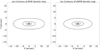 |
Fig. B.1. The mass density comparison between κnfw with qnfw = 0.6 (left panel) and κenfw with qenfw = 0.4 (right panel). The ellipticity implemented in the lensing potential leads to a dumbbell-shaped surface density (see the left panel). In contrast, applying ellipticity directly to κ results in a more physically realistic mass distribution (see the right panel). |
Appendix C: Implementation of the EPL profile
We implemented the surface mass density κepl following Tessore & Metcalf (2015). We define:
 (C.1)
(C.1)
with
 (C.2)
(C.2)
where γ represents the density slope, and rsoft = 0.01″ is the softening radius introduced to prevent divergence at the central pixel. The parameter b is a normalization factor, proportional to the Einstein radius θE, given by
 (C.3)
(C.3)
Appendix D: Joint modeling with ideal kinematic data across varying source grid resolutions
To determine the resolution at which mass model parameter constraints become stable with respect to source grid resolutions, we perform joint modeling assuming MBH = 5 × 10⁹ M⊙. The source grid resolution varies from 58 × 58 to 70 × 70, corresponding to source pixel sizes of approximately 0.05 ± 0.01″ per pixel. We observe that all parameter contours stabilize when modeling with source grid resolutions beyond ∼60 × 60 (see Fig. D.1). Considering the computational time, we conduct joint modeling within the range of 60 × 60 to 68 × 68, excluding 58 × 58 and 70 × 70.
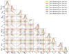 |
Fig. D.1. Equally weighted probability density distributions for all parameters in the joint modeling, given MBH = 5 × 10⁹ M⊙. The joint modeling is performed using different source grid resolutions (represented by different colors) to account for parameter uncertainties induced by variations in pixel size on the source plane. The simulated lensing data are generated assuming a source grid resolution of 64 × 64. |
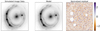 |
Fig. D.2. The best-fit composite mass model, given MBH = 5 × 10⁹ M⊙. The other best-fit model produces similar results. The quasar light in RXJ1131 is very strong, making it difficult to fit. To mitigate its effects, we boost the error in the quasar positions. |
Appendix E: Joint modeling using kinematics data exclude the central bins
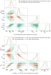 |
Fig. E.1. Comparison between joint modeling using full ideal kinematic data (orange contours) and excluding the central regions (green contours). We observe that uncertainties of parameters are enlarged, but the measurements of Dd and βani move toward the mock input values using the kinematic map excluding the central regions. |
Appendix F: The BIC weight factor  to joint models
Comparison of models on different source resolutions, showing χdyn2 and fBIC*.
All Tables
Comparison of models on different source resolutions, showing χdyn2 and fBIC*.
All Figures
|
Fig. 1. Time comparison between CPU and GPU for extended image modeling of various source resolutions that arecommonly adopted in practice. The computation time is for a single iteration of a source and image intensity reconstruction given the values for lens mass model parameters. The computations took place on a 2.10 GHz CPU and an A100 GPU, respectively. |
| In the text | |
|
Fig. 2. Workflow for the joint modeling using RXJ 1131 as an example. The input datasets consisted of photometric images and the spatial kinematics of the lens galaxy. The red contours in the middle right of the green panel represent the isocontours of both the light and mass density distributions of the lens galaxy, derived from the MGE method (see Sect. 3.2). The modeled Ilight represents the light fitted from optical imaging, and Ilight, IFU corresponds to the light near the spectral absorption lines in the IFU data. In the paper, Ilight is equivalent to Ilight, IFU. We employed an MCMC sampler to simultaneously sample the parameter space ηLD for the lensing and the dynamical modeling. |
| In the text | |
|
Fig. 3. Mock data sets of the lensing imaging and kinematic data. We observed a faint satellite galaxy above the lens galaxy at the same redshift as the lens galaxy. We neglected the satellite when we simulated the IFU data. The satellite is too small to extract useful kinematic information from the IFU datacube other than the redshift (see Shajib et al. 2025). More importantly, based on the previous study, the satellite has a negligible effect on mass modeling and cosmological distance inference (Suyu et al. 2014). The mock IFU data with 52 bins are presented in the same reference frame as the simulated HST imaging. North is up, and east is to the left. |
| In the text | |
|
Fig. 4. Measurements from the joint modeling (combining all mass models) and lensing-only modeling. The shaded contours represent 1σ, 2σ, and 3σ confidence regions. The green contours correspond to the joint modeling using the ideal kinematic data, and the orange contours correspond to the joint modeling using kinematic data with a 5% systematic bias. The gray contours represent the lensing-only modeling. The red box indicates the degeneracy between DΔt, int and λint in the lensing-only modeling. |
| In the text | |
|
Fig. 5. Top panels: Marginalized posterior density distribution of Dd, based on the joint models using ideal kinematic data. The different colors represent posterior densities corresponding to different BH masses, while each color represents five separate posterior distributions that are tightly clustered together, corresponding to models with identical mass parameterizations but different source-grid resolutions. The red color represents EPL mass models, where a small softening scale of rsoft = 0.01″ mimics the presence of a massive BH, eliminating the need to explicitly include an additional MBH. The left panel shows equally weighted Dd posterior densities, whereas the right panel presents the combined Dd posterior density weighted by BIC (see Sect. 3.4). Bottom panels: Marginalized posterior density distribution of DΔt, int, based on joint models using ideal kinematic data. The red dashed lines in both panels indicate the mock input values used in the simulated data. The black dashed lines represent the median values in the BIC-weighted distribution. |
| In the text | |
|
Fig. 6. Best-fit kinematic maps from the joint models for different BH mass assumptions. The displayed kinematic bin maps have 52 bins in total. Upper Panel: Joint modeling is performed using a grid of MBH values ranging from 109 to 1010 M⊙. In each model, the BH mass is fixed and incremented in steps of 109 M⊙ within this range. The best-fit kinematic map, corresponding to MBH = 3 × 10⁹ M⊙, achieves χdyn2 = 50. Middle Panel: The best-fit kinematic map from joint modeling that assumes no BH, yielding χdyn2 = 64. Lower Panel: The best-fit kinematic map from joint modeling using the EPL mass profile, resulting in χdyn2 = 58. |
| In the text | |
|
Fig. 7. H0 and Ωm constraints from our models in a flat |
| In the text | |
|
Fig. 8. Marginalized posterior density distribution of βani based on the joint models using ideal kinematic data. Different colors represent posterior densities corresponding to different BH masses, while the same color indicates models with identical mass parameterization but different source grid resolutions. We observe that as MBH increases, the inferred βani decreases and vice versa. The inferred βani distributions given different MBH spread over the prior range [−0.3,0.3], but different MBH yield different goodness of fit to the kinematic data (as shown in Fig. 5). |
| In the text | |
|
Fig. 9. MBH vs. Dd with 1σ uncertainties based on the ideal kinematic data. This provides a clearer visualization of the upper-left panel in Fig. 5. The plot also illustrates how the BH mass affects the inference of Dd, given that βani is within the prior range of −0.3 to 0.3. The gray shaded region represents models with the BH mass satisfying |
| In the text | |
|
Fig. 10. Constraints on H0 and Ωm from our models in a flat |
| In the text | |
|
Fig. 11. Left: Ideal kinematic data without the bins within −0.15″ to 0.15″ with 43 bins in total. Middle: Best-fit kinematic map with |
| In the text | |
|
Fig. B.1. The mass density comparison between κnfw with qnfw = 0.6 (left panel) and κenfw with qenfw = 0.4 (right panel). The ellipticity implemented in the lensing potential leads to a dumbbell-shaped surface density (see the left panel). In contrast, applying ellipticity directly to κ results in a more physically realistic mass distribution (see the right panel). |
| In the text | |
|
Fig. D.1. Equally weighted probability density distributions for all parameters in the joint modeling, given MBH = 5 × 10⁹ M⊙. The joint modeling is performed using different source grid resolutions (represented by different colors) to account for parameter uncertainties induced by variations in pixel size on the source plane. The simulated lensing data are generated assuming a source grid resolution of 64 × 64. |
| In the text | |
|
Fig. D.2. The best-fit composite mass model, given MBH = 5 × 10⁹ M⊙. The other best-fit model produces similar results. The quasar light in RXJ1131 is very strong, making it difficult to fit. To mitigate its effects, we boost the error in the quasar positions. |
| In the text | |
|
Fig. E.1. Comparison between joint modeling using full ideal kinematic data (orange contours) and excluding the central regions (green contours). We observe that uncertainties of parameters are enlarged, but the measurements of Dd and βani move toward the mock input values using the kinematic map excluding the central regions. |
| In the text | |
Current usage metrics show cumulative count of Article Views (full-text article views including HTML views, PDF and ePub downloads, according to the available data) and Abstracts Views on Vision4Press platform.
Data correspond to usage on the plateform after 2015. The current usage metrics is available 48-96 hours after online publication and is updated daily on week days.
Initial download of the metrics may take a while.