| Issue |
A&A
Volume 701, September 2025
|
|
|---|---|---|
| Article Number | A51 | |
| Number of page(s) | 32 | |
| Section | Planets, planetary systems, and small bodies | |
| DOI | https://doi.org/10.1051/0004-6361/202554894 | |
| Published online | 02 September 2025 | |
The planetary-mass-limit VLT/SINFONI library
Spectral extraction and atmospheric characterization via forward modeling★
1
Laboratoire Lagrange, Université Cote d’Azur, CNRS, Observatoire de la Cote d’Azur,
06304
Nice,
France
2
LIRA, Observatoire de Paris, Univ PSL, CNRS, Sorbonne Univ, Univ de Paris,
5 place Jules Janssen,
92195
Meudon,
France
3
Université Grenoble Alpes, CNRS, IPAG,
38000
Grenoble,
France
4
Max-Planck-Institut fur Astronomie,
Konigstuhl 17,
69117
Heidelberg,
Germany
5
Departamento de Astronomía, Universidad de Chile,
Casilla 36-D,
Santiago,
Chile
6
Aix Marseille Univ, CNRS, CNES, LAM,
Marseille,
France
7
Space Telescope Science Institute,
3700 San Martin Drive,
Baltimore,
MD
21218,
USA
8
NASA-Goddard Space Flight Center,
Greenbelt,
MD
20771,
USA
★★ Corresponding author.
Received:
31
March
2025
Accepted:
25
June
2025
Abstract
Context. Access to medium-resolution spectra (Rλ ~ 1000 − 10 000) at near-infrared wavelengths of young M-L objects allows us to study their atmospheric properties. Specifically, this approach can unveil a rich set of molecular features related to the atmospheric chemistry and physics.
Aims. We aim to deepen our understanding of the M-L transition on planetary-mass companions and isolated brown dwarfs, while searching for evidence of possible differences between these two populations of objects. To this end, we present a set of 21 VLT/SINFONI K-band (1.95–2.45 µm) observations from five archival programs at Rλ ~ 4000. We aim to measure the atmospheric properties, such as Teff, log (ɡ), [M/H], and C/O, and to understand the similarities and differences between objects ranging in spectral type from M5 to L5.
Methods. We extracted the spectra of these targets with the TExTRIS code. We modeled them using ForMoSA, a Bayesian forward modeling tool for spectral analysis, and we explored four families of self-consistent atmospheric models: ATMO, BT-Settl, Exo-REM, and Sonora Diamondback.
Results. Here, we present the spectra of our targets and the derived parameters from the atmospheric modeling process. We confirm a drop in Teff as a function of the spectral type of more than 500 K at the M/L transition. In addition, we report C/O measurements for three companions, 2M 0103 AB b, AB Pic b, and CD-35 2722 b, thereby adding to the growing list of exoplanets with measured C/O ratios.
Conclusions. The VLT/SINFONI Library highlights two key points. First, there is a critical need to further investigate the discrepancies among grids of spectra generated by self-consistent models, as these models yield varying results and do not uniformly explore the parameter space. Second, we do not observe any obvious discrepancies in the K-band spectra between companions and isolated brown dwarfs, which suggests that these super-Jupiter objects might have formed through a similar process; however, this possibility warrants further investigation.
Key words: planets and satellites: atmospheres / planets and satellites: composition / planets and satellites: formation / planets and satellites: gaseous planets / planets and satellites: general
Based on observations collected at the European Organisation for Astronomical Research in the Southern Hemisphere under ESO programs 092.C-0535(A), 092.C-0803(A), 092.C-0809(A), 093.C-0502(A), and 093.C-0829(A&B).
© The Authors 2025
 Open Access article, published by EDP Sciences, under the terms of the Creative Commons Attribution License (https://creativecommons.org/licenses/by/4.0), which permits unrestricted use, distribution, and reproduction in any medium, provided the original work is properly cited.
This article is published in open access under the Subscribe to Open model. This email address is being protected from spambots. You need JavaScript enabled to view it. to support open access publication.
1 Introduction
The discovery of the brown dwarf Teide 1 by Rebolo et al. (1995) marked a milestone in astronomy, as it was the first confirmed object of its kind. A decade later, this was followed up by first direct image of a giant exoplanet 2M1207 b by Chauvin et al. (2004). Remarkably, these two objects share the same spectral type (M9), highlighting from the start the challenge in distinguishing between a planet and a brown dwarf. Initially, the distinction between giant planets and brown dwarfs was defined by a mass threshold (Kumar 2002), with dividing lines at ~13.6 MJup and ~75 MJup, corresponding to the limits for deuterium and hydrogen fusion, respectively (Burrows et al. 1997; Chabrier 2005; Hayashi & Nakano 1963). However, uncertainties remain regarding the Deuterium boundary (Spiegel et al. 2011; Mollière & Mordasini 2012) and we also know of isolated objects with masses below 13.6 MJup. Therefore, a more detailed definition is needed to classify exoplanets and brown dwarfs.
In this context, an alternative approach is through classifying these objects based on their formation pathways (Chabrier et al. 2014), which offers a physically meaningful distinction since formation processes relate to the origin and nature of these bodies. Objects near the planetary-mass limit can form through three main mechanisms: they can form by the direct-gravitational collapse of a molecular cloud (e.g., stars), but without sufficient mass for sustained fusion (Padoan et al. 2005), and in such cases, they would be classified as brown dwarfs. Alternatively, they may form within the gravitational influence and from the protoplanetary material of a newly formed star. These exoplanets could emerge through a rapid, top-down process, such as gravitational instabilities (Boss 1997), or a slower, bottom-up mechanism, such as core or pebble accretion (Pollack et al. 1996).
Numerous studies have explored and probed the overlapping regime between brown dwarfs and planets, as done by Leconte et al. (2009), Faherty et al. (2013), Bonnefoy et al. (2014), Biller (2017), and Nielsen et al. (2019), among others. From such studies, it has been suggested that brown dwarfs can be considered as exoplanet analogues; however, we also know that they were likely formed through different mechanisms. Different formation pathways are expected leave behind distinct imprints on their atmospheres, which we could potentially measure. An early approach in this direction was based on the assumption that the value of the carbon-to-oxygen ratio (C/O) could serve as a proxy for the formation location of an exoplanet (Öberg et al. 2011; Madhusudhan 2012). This was later extended to other elements such as the nitrogen-to-oxygen (N/O) or nitrogen-to-carbon (N/C) ratios (Cridland et al. 2017; Turrini et al. 2021) and the refractory-to-volatile ratio (Lothringer et al. 2021). More recently, studies such as Mollière & Snellen (2019) and Gandhi et al. (2023) have suggested that isotopic ratios of elements like hydrogen, carbon, oxygen, and nitrogen could provide even tighter constraints to planet formation models. It has also been proposed that the overall system’s architecture can provide insights into the formation mechanisms as well (e.g., Desgrange et al. 2023).
To better understand these connections, many studies have focused on directly characterizing the imaged objects at the planetary-mass limit, spanning spectral types from T to M, using instruments that operate at low-to-medium spectral resolutions within the wavelength range of ~0.5 to ≳2.5 µm. For example, the NIRSPEC instrument at Keck has been used for several brown dwarf studies, including the 17 targets observed by Rice et al. (2009) and the 228 targets observed by Martin et al. (2017). Additionally, the X-Shooter instrument at the Very Large Telescope (VLT) has been proven efficient for studying young, low-gravity objects, as evidenced by the observations of 9 targets by Petrus et al. (2020) and 20 targets by Manjavacas et al. (2019). The instrument used in this study is SINFONI, located at the VLT. It has been employed in previously published libraries, such as the nine targets observed by Patience et al. (2012) and the 15 targets observed by Bonnefoy et al. (2014). In this context, we can expect to see more such libraries in the near future, for example, for such instruments as ERIS, GRAVITY+, and CRIRES+ at the ESO/VLT as well as ESO/VLTI itself.
Even though we are now in an era where we have obtained (and continue to gather) extensive data, it has been shown in atmospheric (e.g., Mollière et al. 2022) and protoplanetary disk studies (e.g., van der Marel & Mulders 2021) that the overall picture is far more complex than initially anticipated. In fact, most studies converge on a critical point: further homogeneous characterization of exoplanets is essential for enabling robust statistical analyses of their properties, which are crucial for understanding how these planets formed and evolved (e.g., Marleau et al. 2019; Petrus et al. 2021; Wang et al. 2021; Hoch et al. 2023; Palma-Bifani et al. 2023). In light of this, it is worth asking whether the ongoing search for parameters that can trace formation pathways remains effective. A more meaningful approach may lie in consistently modeling the spectra of diverse exoplanets and planetary analogues using uniform assumptions and observational strategies. In this way, we can begin to unravel the true complexity of their formation histories.
In this spirit, we identified a previously overlooked dataset of planetary-mass objects observed with the VLT/SINFONI instrument dating back to 2014. This rich dataset includes observations of young companions and isolated objects near the planetary mass limit. We begin this paper by presenting the sample and giving a detailed description of the observations, data reduction, and spectral extraction process in Section 2. In Section 3, we outline the forward modeling approach and describe the atmospheric models used in our study and our fitting strategy. The main results are reported in Section 3.4, with our interpretations given in Section 4. We present our conclusions in Section 5.
2 The VLT/SINFONI observations
We identified an archival library of medium-resolution K-band spectra. The corresponding observing programs were executed a decade ago, but no work has fully presented or homogeneously characterized this dataset to date. In this section, we first describe the SINFONI instrument in Section 2.1. We characterize the selected sample of objects in Section 2.2 and outline the data reduction steps in Section 2.3. Finally, we present the complete compilation of the SINFONI Library spectra in Section 2.4.
2.1 The SINFONI instrument
SINFONI is an integral field spectrograph (IFS) that was operational at the European Organisation for Astronomical Research in the Southern Hemisphere (ESO) from 2004 to 2021. It was decommissioned in 2021 and replaced by the ERIS instrument, which shares similar properties in terms of its IFS configuration. It combined two primary subsystems: the adaptive optics (AO) module known as MACAO and the IFS known as SPIFFI. This configuration enabled the simultaneous spectroscopy of 32×64 spatial pixels (spaxels) with a medium spectral resolving power. SINFONI covered the near-infrared atmospheric windows (J: 1.1–1.4 µm, H: 1.45–1.85 µm, and K: 1.95–2.45 µm) with the additional capability to observe the combined H+K bands at a lower spectral resolution.
The SPIFFI spectrograph utilized an image slicer to divide the field of view (FoV) into 32 slices (slitlets) and rearranged them into a one-dimensional (1D) pseudo-slit, dispersed onto a two-dimensional (2D) 2048×2048 pixel Hawaii Rockwell focal plane array (Eisenhauer et al. 2003). Four gratings, corresponding to the J, H, K, and H+K bands, were made available, with spectral resolution influenced by the selected pre-optics. The FoV was recomposed spatially into rectangular spaxels, with plate scales of 0.25/0.1/0.025 arcsec/pixel, offering a resolution of 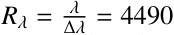 , 5090, or 5950, respectively, in the K-band.
Regarding the performance, the line spread function (LSF) of SINFONI varied with plate scales and gratings due to differences in how the pre-optics illuminated the gratings. A Nyquist sampling was not achieved in all modes, necessitating a careful calibration to ensure accurate spectral resolution. The Hawaii 2RG detector also exhibited persistence effects, even when illuminated at levels below saturation. This limitation required meticulous calibration to mitigate artifacts and maintain data quality.
2.2 The sample
The observations used in this work are part of an archival library of medium-resolution VLT/SINFONI K-band spectra, observed approximately a decade ago as part of five different programs: 092.C-0803(A) and 093.C-0829(A&B) (P.I.: Kopytova), 093.C-0502(A) and 092.C-0535(A) (PL: Radigan), and 092.C-0809(A) (P.I. Patience). In the appendix, Table A.1 provides the observational log, detailing parameters such as the number of exposures per sequence, integration times (DIT), and the number of integrations per exposure (NDIT), as well as the airmass and seeing ranges for each night.
While SPIFFI is an essential component of SINFONI, the use of MACAO, the adaptive optics (AO) system depends on the observational strategy (seeing-limited versus diffraction-limited). In Table A.1, we show that MACAO was off when the observations of the isolated targets and FU Tau b were taken, as these objects are not contaminated by the presence of a bright star close by. For the remaining companions, MACAO was utilized, with the host star serving as a natural guide star (NGS) for wavefront sensing and generally providing a better signal-to-noise ratio (S/N). Furthermore, different plate scales were used for the various targets, which impacted the choice of aperture radius and the true spectral resolution. In addition, for each science target, a telluric standard star (STD) was observed immediately before or after each sequence to ensure a proper telluric contamination subtraction.
The selected sample consists of 21 planetary-mass objects, as listed in Figure 1. A broad overview of previous studies and the characteristics of each target is available in Appendix B. The sky map displayed in Figure 1 was generated using the mw-plot Python package1. Figure 1 illustrates that the sample primarily comprises two architectures: directly imaged companions (targets ending by letter b) and isolated brown dwarfs. All our targets are young (1–30 Myr) and predominantly located in two star-forming regions: Taurus and Upper Scorpius (Sicilia-Aguilar et al. 2013; Torres et al. 2008). The exceptions are the four companions marked in yellow, which are recognized members of the β Pictoris, Carina, AB Doradus, and Tucana-Horologium moving groups (Zuckerman & Song 2004; Zuckerman et al. 2004; da Silva et al. 2009). In terms of distance, all objects are within 150 pc from the Sun and visible from the Chilean Atacama desert, where the Very Large Telescope (VLT) is located.
In general, depending on the sky location, we would expect different amounts of interstellar dust to cause extinction, which we have estimated based on the Gaia 3D extinction map from Lallement et al. (2022). The colors in Figure 1 correspond to the amount of interstellar extinction (Av), revealing three distinct groups: The scattered companions have Av values smaller than 0.001 magnitudes, the targets at the Taurus region have values between 0.05 and 0.25 magnitudes, and the targets at the Upper Scorpius regions have values between 0.25 and 0.35 in magnitude, except for USco 1606-2219 and USco 1610-2239, whose extinctions are lower (see Table A.2). in Table A.2, together with the visible interstellar medium extinction (Av), we report all the aforementioned information, such as the right ascension (RA), declination (Dec), association, parallax, distance to us, and age for each target.
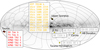 |
Fig. 1 Sky map showing the right ascension and declination curves, along with our 21 targets. The circle marks represent companions, while the star marks indicate isolated objects. The names of the different associations are indicated in black. |
2.3 Data reduction and calibrations
We processed the raw data with the SINFONI handling pipeline v3.0.02 through the EsoReflex3 environment. The SINFONI pipeline utilizes calibration frames (darks and flats) to perform basic adjustments on the raw science frames, correcting for bad pixels and pixel-to-pixel sensitivity variations as a function of wavelength. In practice, the pipeline identifies the slitlet positions on the frames via Gaussian fitting at each wavelength. From this, a data cube is built for each exposure, correcting for spatial and spectral distortion, as shown in Figure 2.
Further corrections, including wavelength calibration, sky subtraction, and telluric removal, were necessary to extract a spectrum for each target. In this study, we employed the Toolkit for Exoplanet deTection and chaRacterization with IfS (TEx-TRIS) code, similarly to the way it has been used in previous works, such as Petrus et al. (2021); Palma-Bifani et al. (2023); Kiefer et al. (2024). Hereafter, we detail the steps and specific post-processing techniques applied to extract the spectra from each data cube.
We began by performing a wavelength calibration for each exposure using the OH emission lines. Across the datasets, we identified constant spaxel-to-spaxel wavelength shifts of up to approximately 15 km/s relative to the telluric absorption lines. We employed a cross-correlation method within a defined wavelength interval to correct these wavelength shifts and determine the offsets in a sequence of SINFONI data cubes. Then, we applied this offset to correct the corresponding cube wavelength solutions in the same way for the science and standard star cubes.
Before applying additional corrections, the exact position of each object’s PSF center in each data cube had to be determined. We measured the motion of the point source affected by atmospheric refraction by fitting a 2D Moffat function, recovering the center coordinates in each cube as a function of spaxels and wavelength. The wavelength dependency of the PSF center’s motion is smooth and can be approximated by a polynomial of degree 2. This approximation allowed us to bin the data in wave-length before estimating the center position, thereby reducing the computation time. For the science objects, we binned every ten points, while for the standard stars (which are brighter), we binned every 100 points.
We observed that sky emission lines heavily contaminated several of our data cubes. To correct for this contamination (and because the sky emission lines are wavelength-dependent), every spaxel had to be corrected equally. The degree of sky emission contamination was estimated from empty sky regions. For this, we applied a ring mask around the object with a large inner radius to ensure we were not capturing any wing of the object’s PSF. We manually adjusted the inner and outer radii for each case and masked out all other elements. We applied an additional border mask when the object was near a border. We then measured the median value among the spaxels of the selected sky portion and subtracted this median from each spaxel, repeating the process for all wavelengths. When the sky emission is low, this correction subtracts zero from every spaxel, but when it is high, it suppresses the lines. We applied this correction only to the science data cubes.
Next, we were ready to select an aperture radius and extract the spectra from the science and standard star data cubes. We extracted a spectrum with error bars within a circular aperture in an IFU data cube. The error bars were computed from the estimated level of residuals around the circular aperture. For this, we used the photutils4 Python package, specifically the CircularAperture function. We fixed the aperture radius at 5 pixels for the standard star cubes. For the science cubes, we estimated the optimal aperture radius, which depends on several factors, including the plate scale and MACAO usage, and we maximized the S/N of our data by performing spectral extractions with aperture radii ranging from 1 to 12 pixels (in integer increments). This approach allowed us to optimize the radius selection later on.
The preliminary spectrum of each data cube (both science and standard star) shows contamination by water bands from the Earth’s atmosphere. To address this, we obtained a spectrum of the atmospheric transmissions for all nights using the standard star observations. First, we corrected the standard star spectrum by removing the features of near-infrared hydrogen and other stellar lines. We identified and interpolated these lines across the affected spectral ranges. Next, we used the standard star’s spectral type as input to calculate its effective temperature (Teff) and then computed a blackbody spectrum at that specific Teff. We derived a telluric spectrum by dividing the corrected standard star spectrum by the corresponding blackbody spectrum. Finally, we divided the telluric spectrum for each data cube, effectively removing telluric contamination from the science observations. We applied the same step to each data cube and each spectral extraction, varying the aperture radius. We then applied a Barycentric correction to each corrected spectrum computed using the hellcor function of the Python PyAstronomy library (Czesla et al. 2019).
At this stage, we had 12 corrected spectral extractions for each observation of each target. We chose to use AB Pic b as an example target, as described henceforth. Under ideal conditions, we can assume that the full width at half maximum (FWHM) of the target’s PSF can be approximated by a Gaussian. For AB Pic b, a bright target, the FWHM is approximately 5 pixels, so we could select this aperture radius, as done in Palma-Bifani et al. (2023). However, the FWHM can vary significantly with the considered plate scale, the seeing, MACAO’s setup, and other factors. Therefore, having an objective criterion for selecting the best aperture radius becomes important to ensure that our extracted spectra for all 21 targets have the best possible quality. To select the best aperture radius, we proceeded as follows. In the wavelength range from 2.05 to 2.2 µm, we know that M to L spectral type targets exhibit a positive-to-zero slope. Therefore, we fit a first-order polynomial to the data and analyze how the slope varies as a function of the aperture radius. The left panel of Figure 3 illustrates this. Each color represents a different exposure of AB Pic b. In general, we observe that for most observations, the slope exhibits two distinct behaviors: for small aperture radii, it increases rapidly; however, beyond a critical radius, the rate of change of the slope decreases.
Building on this criterion, we can go further. Specifically, we estimated an S/N that was in the same spectrum wavelength range for each exposure. In the central panel of Figure 3, we observe that the S/N initially increases until it reaches a maximum value and then decreases. This behavior arises because, for small radii, not all of the PSF signal is captured within the aperture; consequently, both the signal and noise remain low. As the aperture radius increases, more planetary flux is included, raising the S/N. However, background contamination becomes dominant when the aperture radius is too large, thereby reducing the S/N. The central panel of Figure 3 illustrates this behavior. As an example, in the central panel of Figure 3, we added a square symbol to mark the aperture radius that maximizes the S/N, which is selected as the final aperture radius. This applies to all targets and datasets.
With the described criterion, we could select the aperture radius, but the quality of the SINFONI observations varies from dataset to dataset. Some datasets exhibit behaviors that are clearly driven by systematic errors, such as wiggles in the spectra or discontinuities in the slope as a function of aperture radius. In this sense, we also implemented a rejection criterion. We computed the derivative of the slope as a function of the aperture radius, as shown in the right panel of Figure 3. If this derivative was not monotonically decreasing, we rejected the dataset. For AB Pic b, this led to the rejection of the entire second night of observations. For some targets, we relaxed the criterion with a threshold, especially when MACAO was not used.
Finally, we median-combined the accepted spectra to create the final spectrum for each target. We report the corresponding errors as the standard deviation across the included datasets. For each target, we then calibrated the extracted normalized spectrum in flux units (W m−2 µm−1) using the K-band magnitude values reported in Table A.3 and the VLT/NaCo Ks filter, as previously done in Palma-Bifani et al. (2023). We report the flux factor used to multiply the normalized spectra to recover them in apparent flux units in Table A.3.
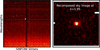 |
Fig. 2 Example of the first exposure of AB Pic b: the SINFONI raw observation (left), where each spectral slice (slitlet) is projected as vertical lines, compared to the reduced data cube delivered by EsoReflex for which we show the slice at λ = 1.95 (right), which shows a clear detection of the source at the center. |
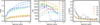 |
Fig. 3 Example of optimal aperture radius selection and spectra rejection criteria using the AB Pic b dataset. In each panel, each color represents a different exposure of AB Pic b. Left: values for the fitted continuum slope between 2.05 and 2.2 µm as a function of aperture radius. Two distinct domains are observed: for radii smaller than the optimal value, the slope increases steeply; for radii larger than the optimal value, the slope still varies but becomes more stable. Center: S/N estimated within the same wavelength range as in the left panel, plotted as a function of aperture radius. For each observation, we highlighted the maximum S/N value with a square. The aperture radius corresponding to this maximum is our final selected radius each time. Right: derivative of the slope (reported in the left panel) with respect to the aperture radius. Some targets exhibit a non-smooth, decreasing derivative; we reject those epochs. For AB Pic b, this resulted in the rejection of the entire dataset for the second night. |
2.4 The SINFONI library
When we refer to the SINFONI library we mean the collection of 21 reduced and corrected K-band spectra of planetary-mass companions and isolated targets. The entire SINFONI library is shown in Figure 4. The library is organized by spectral type, from earlier to later types, as indicated by the color of each spectrum, labeled on the right. The whole collection of spectra is available together with this publication for public use.
From Figure 4, we see that some targets appear “noisier,” as is the case with most of the Upper Scorpius (USco) targets. This is the result from observing without MACAO and using the largest plate scale, meaning that the FWHM of the PSF is larger, leading to observations with a lower S/N. For example, we can also see that FU Tau b’s spectrum exhibits many “emission” lines. However, we note that these are not real emission lines from the companion but artifacts from imperfect OH-sky emission line correction, given that the FU Tau b observations are heavily contaminated. Targets observed with MACAO and in long exposure sequences (such as CD-35 2722 b, observed with an intermediate plate scale and exposures of 150 seconds) exhibit very stable behavior, resulting in a high S/N spectrum.
In addition to the spectra, we have summarized the general properties of the sample in Tables A.2 and A.3. These tables include the Gaia DR3 parallaxes (Gaia Collaboration 2023), the corresponding distances in parsecs, and the expected interstellar medium extinction values derived from the 3D maps of Lallement et al. (2022). We also provide the age, spectral type, apparent and absolute K-band magnitudes, flux, and all the references used for each target. To complement this information, we have used the age and absolute magnitudes, along with the BHAC 15 evolutionary models (Baraffe et al. 2015), to compute predictions for key properties. Specifically we employed both the DUSTY and COND versions of the BHAC15 models to estimate the expected effective temperature, surface gravity radius, and mass, reported in Table A.5. Having introduced our library, we proceed to further understand the main physical properties of these objects by characterizing the atmospheric properties of this sample.
3 Atmospheric modeling
In the community we typically encounter two approaches to modeling exoplanet atmospheres: the forward problem and the inverse modeling problem. These two methods can be seen as addressing the Bayesian problem from opposite directions, which, due to Bayes’ theorem, are perfectly equivalent. Our work here focuses on the forward modeling problem. In other words, we examine existing families of models, which are typically parameterized by a few variables. Some advantages of this approach are that the modeling process remains self-consistent and the computational cost for medium-resolution observations remains reasonable. We present our modeling framework in Section 3.1. We then describe the grids of models we implemented in Section 3.2 and our fitting strategy for modeling and analyzing the entire SINFONI library in Section 3.3.
3.1 ForMoSA
To model exoplanetary atmospheres and understand their physical and chemical processes, we used ForMoSA5, an open-source Python package developed within our group (ForMoSA Collaboration et al., in prep.). It has already been extensively used and described in various works, such as Petrus et al. (2021); Palma-Bifani et al. (2023); Petrus et al. (2024); Palma-Bifani et al. (2024), as well as in our ReadTheDocs6 documentation page.
In its simplest form, ForMoSA receives as input a set of observations, a specific grid of models, and a configuration file. First, ForMoSA adapts the grid of models to match the wave-length distribution of the observations. Then, ForMoSA performs a nested sampling parameter exploration, for which in this work, we selected the Pymultinest7 sampler with 500 live points. Finally, ForMoSA saves the outputs and includes a plotting module that allows quick visualizations and provides access to all inputs, parameters, and variables. In this regard, ForMoSA also enables an exploration of the posterior distribution of a selection of additional parameters, such as the radial velocity, rotational velocity, interstellar medium extinction, and the radius of the target, to better adapt the models to the data.
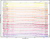 |
Fig. 4 Final extracted spectra for each of the 21 targets in the sample, organized and colored by their spectral type reported in the literature (see Table A.3). The errors are reported in gray, and the main absorption features are labeled at the top of the figure, also in gray. On the right, we annotate the flux scaling factor for each target in units of W m−2 µm−1, also reported in Table A.3. |
3.2 Self-consistent grids of atmospheric models
Currently, several efforts are underway in our community to develop atmospheric models. Each of these efforts makes different assumptions and simplifications. While different groups share their models as parameterized grids, these grids often have distinct features and explore varying parameters across different ranges. Comparing these grids is essential, as demonstrated by Petrus et al. (2024), who extensively modeled the atmosphere of VHS 1256 b observed with NIRSpec and MIRI on JWST (Miles et al. 2023). The models implemented on that study included ATMO (Tremblin et al. 2015, 2017), BT-SETTL+C/O (Allard et al. 2012), Exo-REM (Charnay et al. 2018), Sonora Diamondback (Morley et al. 2024), and DRIFT-Phoenix (Helling et al. 2008).
Here, we propose a similar approach; however, instead of having a broad wavelength range as in the observations of VHS 1256 b, we focus solely on the K-band and model these observations homogeneously for the 21 targets in our sample. For this, we use five different grids: ATMO, two versions of BT-Settl (with and without exploring the C/O ratio), Exo-REM, and Sonora Diamondback. A comparison of the parameter space explored by each of these grids is provided in Table 1. The spectral resolutions in the last column were estimated, assuming that the synthetic spectra are Nyquist sampled. Hereafter, we provide a brief description of each grid.
ATMO (Tremblin et al. 2015, 2017): One of the main characteristics of the ATMO models, which differentiates them from other grids, is that they do not consider clouds. The authors demonstrate that cloudless atmospheric models, which assume a temperature gradient reduction caused by fingering convection, provide a very good model for reproducing NIR spectra. This spectral window is dominated by molecular features from H2O, NH3, CH4, and CO. Therefore, the models focus on non-equilibrium chemistry processes occurring at the L-T and T-Y transitions, including CO/CH4 and N2/NH3, as described in Venot et al. (2012). Differences in mean molecular weights across atmospheric layers can drive fingering convection (mixing two liquids with different densities), which reduces the temperature gradient between layers. This effect can be modeled using the adiabatic index parameter (γ), explaining the reddening observed in low-mass objects. In these models, mixing length theory is used to describe convective mixing. Additionally, the models include Rayleigh scattering from H2 and He, and assume chemical equilibrium among 150 species, including 30 condensates, which are modeled by minimizing the Gibbs free energy. Finally, the radiative transfer is solved using the line-by-line approach described in Amundsen et al. (2014), with the correlated-k method employed to enhance computational efficiency.
BT-Settl and BT-SETTL+C/O (Allard et al. 2012; Allard 2014): The BT-Settl models originated in the stellar modeling community and were later extended to lower temperatures. For this extension, non-equilibrium chemistry was incorporated similarly to ATMO, but without the parametrization for fingering convection. For the chemistry, solar abundances were adopted from the revised values of Asplund et al. (2009). The Rossow (1978) cloud model was implemented, incorporating radiation-hydrodynamical simulations of mixing under hydrostatic equilibrium, which allows for supersaturation and mixing processes. This framework enables the modeling of the stellar-substellar transition by comparing the timescales of condensation, sedimentation, and mixing (extrapolated from convective velocities into stable layers), while ignoring coalescence and coagulation. The models assume efficient nucleation for 40 species, and the radiative transfer through the atmosphere is solved using the PHOENIX atmospheric code (Hauschildt et al. 1997; Allard et al. 2001). The most extensive version of the BT-SETTL grid spans a wide temperature range, from 70 000 K for stars to 400 K for young planets. However, the versions used here were truncated to match the Teff of interest, and BT-SETTL+C/O also explores the C/O ratio as an additional parameter. An observed limitation of BT-Settl is that it does not allow for sufficient dust formation in brown dwarf atmospheres due to a conservative supersaturation threshold. This results in a persistent offset when reproducing the spectra of ultra-cool objects.
Exo-REM (Baudino et al. 2015, 2017; Charnay et al. 2018; Blain et al. 2021): The Exo-REM models are based on radiativeconvective equilibrium with a simplified treatment of cloud microphysics relatively similar to BT-SETTL+C/O. They incorporate opacities for collision-induced absorption by H2 and He, as well as nine molecular and atomic species, and solar abundances as defined by Lodders (2010). For these models, atmospheric vertical mixing is parameterized using a fixed eddy mixing coefficient for a cloud-free environment, with clouds subsequently added on top of it. Similar to ATMO and BT-Settl, Exo-REM includes non-equilibrium chemistry, particularly relevant in cooler and metal-rich atmospheres where vertical mixing dominates. The Exo-REM models also account for clouds composed of Fe and Mg2SiO4, modeled using a simplified microphysics approach. Cloud particle radii are determined by comparing the timescales for condensation growth, coalescence, vertical mixing, and sedimentation with the shortest timescale process governing the particle size. A single representative radius is assumed for all cloud particles (Rossow 1978), with particle growth limited by removal through sedimentation or mixing. The primary advantage of Exo-REM lies in its computational efficiency and its ability to explore non-solar metallicities.
Sonora Diamondback (Morley et al. 2024): The Sonora Diamondback grid is a recent addition to the SONORA family, which also comprises the SONORA-Bobcat (Marley et al. 2021), SONORA-Cholla (Karalidi et al. 2021), and SONORA-Elf-Owl (Mukherjee et al. 2024) models. The Sonora Diamondback models are based on the radiative-convective equilibrium frame-work described in Marley & McKay (1999), with vertical mixing modeled using mixing-length theory. Sonora Diamondback includes opacities for 15 molecules and atoms (e.g., silicates, sulfides, salts, Fe, and H2O), as well as collision-induced absorption by H2 and He, with atmospheric chemistry set to solar abundances (Lodders 2010). Sonora Diamondback include clouds, but unlike all previously presented grids, chemical equilibrium is assumed throughout the atmosphere. Clouds in Sonora Diamondback are parameterized using the approach of Ackerman & Marley (2001), where sedimentation efficiency is controlled by the ƒsed parameter. Unlike Exo-REM, this cloud parametrization assumes that at each vertical level, particle size evolves by matching the timescale of mixing to the timescale of sedimentation. This parameterization allows the model to span a wide range of cloud conditions, from entirely clouded (ƒsed = 1) to nearly cloudless (ƒsed = 8) atmospheres. The SONORA family of models is notable for its high spectral resolution and flexible cloud modeling, allowing for accurate simulations of various atmospheric conditions, particularly for cooler substellar atmospheres. However, the assumption of chemical equilibrium throughout the atmosphere limits its ability to capture non-equilibrium processes, often crucial for atmospheres with substantial vertical mixing.
As observed, each family of models adopts different assumptions and explores a distinct set of parameters, as illustrated in Table 1. While all models achieve resolutions equal to or higher than the SINFONI data and consistently explore Teff and log (ɡ) as free parameters, their parameter space coverage varies significantly. From the Teff ranges presented in Table 1, we note that the lower limits of the grids extend below the expected temperature range for our library (between 1500 K and 2500 K, expected for spectral types from L5 to M5). However, the upper limits of the grids vary: only ATMO and BT-SETTL+C/O extend sufficiently high to encompass this range fully. The other grids have trun-cated Teff ranges, which may not cover the hottest objects in our sample. This limitation means that we cannot use all grids for all targets despite our aim for a homogeneous analysis. Instead, our fitting approach must account for these discrepancies, as further described in the following section. Moreover, the differences in model assumptions, such as the treatment of clouds, chemical equilibrium, and vertical mixing, further emphasize the need to carefully interpret the results and consider each grid’s specific strengths and weaknesses in the context of our data.
Comparison of the different grids of atmospheric models.
Summary of processing times and mean  for the different model configurations.
3.3 Fitting strategy
When performing an atmospheric parameter exploration with ForMoSA, the first thing that becomes evident is that the posterior distributions vary depending on the chosen combination of parameters. For a preliminary exploration of the entire sample and to address questions such as how Teff and log (ɡ) behave and whether the solutions are physically consistent, we repeated the modeling with different setups. In these setups, we systematically increased the number of free parameters explored. We began with only the grid parameters, then incrementally added parameters such as radial velocity (RV), a spectral line broadening factor (β), interstellar medium extinction (Av), and various combinations of these parameters, considering their physical significance. These setups were labeled from v01 to v07 in Table 2. Hereafter, we revisit the meanings of RV, β, and Av as additional free parameters.
The RV parameter represents a Doppler shift applied to the spectrum, corresponding to the absolute Doppler shift of spectral lines caused by the target’s motion relative to the solar system. The derived RV value includes both a system component and a planet for gravitationally bound targets. In our sample, more than half of the objects are isolated but belong to young associations and moving groups. We use the RV parameter in our analysis because it is necessary for the models to accurately reproduce the depth of certain spectral lines.
The spectral line broadening factor, denoted as β, is a parameter introduced to account for broadening effects in spectral lines, such as those caused by a planet’s rotation. This parameter can only be explored together with RV. In this context, β equals the v sin(i) parameter used in Palma-Bifani et al. (2023). However, the ability to measure the impact of projected rotational velocity on spectral lines depends on the spectral resolution of the observation. The minimum measurable value is inversely proportional to the spectral resolution, given by the relation βmin = c/Rλ, where c is the speed of light. For SINFONI observations, as mentioned earlier, the spectral resolution varies between 4490 and 5950, depending on the plate scale. Additionally, the SINFONI user manual specifies that its detector undersamples the observations. Thus, the true spectral resolution of the data is governed by the Nyquist sampling of the spectral points, which is approximately 4000 for the shortest wavelengths and 5000 for the longest. At a resolution of 4000, βmin is about 75 km/s. This implies that, for this dataset, we cannot measure any spectral broadening smaller than 75 km/s – an unrealistically high threshold for most planets’ rotation velocities. In Palma-Bifani et al. (2023), the authors reported a v sin(i) value of 73 km/s for AB Pic b. However, we have now revised this and identified that this value is only an upper limit. Despite this limitation, we still fit within ForMoSA for β as a free parameter because, along with the RV parameter, it aids in accurately fitting the depths of the CO bands. This, in turn, enables an accurate fitting of the CO features and, consequently, reliable measurements of the C/O ratio for some of our targets. When fitting for β in ForMoSA, we use a fixed limb-darkening coefficient of 0.6, which is reasonable for young, low-mass objects Claret (1998).
Next, we consider the interstellar medium extinction (Av). To explore Av in ForMoSA, we use the extinction.fm07 package8, which implements the Fitzpatrick & Massa (2007) extinction model. Since our targets are members of young associations, interstellar dust can cause non-negligible extinction, potentially affecting the spectral slope for some of them. For this reason, we initially explored this parameter freely. However, we noticed that allowing Av to vary freely could significantly impact the derived Teff values by more than 1000 K. This effect is illustrated in Figure 5, which shows results for the ATMO models, but it is worth mentioning that this behavior is not grid dependent. In the upper panel of Figure 5, we compare the derived Teff and log (ɡ) values for model runs v01 to v04. The dashed lines connect the estimates from v01 to v04. When Av is freely explored, the models often select very high values (up to more than 5 magnitudes), leading to substantial biases in the derived Teff and log (ɡ). To mitigate this issue – while still accounting for the importance of Av for some targets – we decided in run v07 to use a fixed interstellar extinction value in ForMoSA, denoted as  . These values are derived from the accurate 3D extinction maps, thanks to the Gaia Data Release 3 (Lallement et al. 2022). We report the estimate for each of our targets in Table A.2. The lower panel of Figure 5 compares the results of model runs v03 and v07. This comparison shows that, for most targets, the Teff values remain stable when comparing no extinction to fixed extinction. However, as expected, the fixed Av adjusts the posterior distributions for some targets, demonstrating the importance of adequately accounting for interstellar extinction.
We performed the ForMoSA exploration using uniform priors across the entire parameter range defined by each grid. We also used uniform priors for the RV and β, exploring values between −100 and 100 km/s and 0 and 500 km/s, respectively. As mentioned above, for Av, we initially applied uniform priors between 0 and 15 magnitudes. However, we later fixed this parameter to the values reported in Table A.2. Additionally, and specifically for run v08, we employed informed Gaussian priors for the surface gravity. This decision was made because, as demonstrated in Palma-Bifani et al. (2024), using informed priors for the case of AF Lep b helped recover a physically consistent solution and overcome the so-called “radius problem”, often observed when modeling the atmospheres of directly imaged companions. Here our informed prior was constructed by using the log (ɡ) and its associated error, estimated from the BHAC15 COND03 evolutionary models, described above and reported in Table A.5), as the mean and variance for a Gaussian prior (𝒩(µ, σ2)). The exception was for BT-Settl, where we loosened the restriction to 10 × σ for the variance, otherwise, the prior was overly constraining and resulted in extremely long convergence times (over 12 hours for a single target) compared to the previous runs (see times of convergence reported in Table 2).
In Figure 6, we show an example of the impact of this prior using the case of AB Pic b, illustrating how the posterior distributions differ between the v07 and v08 runs. We observe that the v07 run resulted in a very high log (ɡ) of ~4.9 dex. This value is unrealistic, as the evolutionary model predictions point to a ~4 dex solution, marked by the blue cross in the figure. The impact of adding this prior is particularly evident in the retrieved values for [M/H] and the C/O ratio. With the log (ɡ) prior, we recover solutions much closer to stellar values (indicated by the black stars) compared to the results without the prior. This behavior is observed only for HIP 78530 b and USco 1606 2335, in addition to AB Pic b, while the other targets in the sample already have realistic log (ɡ) posteriors in the v07 runs. However, for consistency and because adding this constraint does not negatively affect the solutions, we report the v08 runs for all targets in the results presented hereafter.
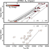 |
Fig. 5 Exploration of the impact of Av on the derived posterior values of Teff and log (ɡ) for the ATMO grid of models. The Av value is indicated by the color of each symbol. In the top panel, we compare Teff and log (ɡ) from model runs v01 (Av = 0) and v04 (Av freely explored). Dashed lines connect the estimated values for a single target across the two runs. This shows that both Teff and log (ɡ) are highly degenerate with Av. In the lower panel, we perform a similar comparison between model runs v03 (Av = 0) and v07 ( |

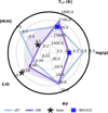 |
Fig. 6 Comparison of the posterior distributions using a uniform versus Gaussian prior on log (ɡ) for AB Pic b (v07 vs. v08 model predictions, shown in light blue and purple, respectively). The Gaussian prior mean value is marked with a blue cross on the log (ɡ) axis, based on the BHAC15 and COND03 evolutionary model predictions. We also marked the Teff predictions with a blue cross, although this was not used as prior information. For comparison, the solar values for [M/H] and the C/O ratio are shown as black stars. |
3.4 Atmospheric modeling results
To summarize, Table 2 provides an overview of all the model runs performed to explore the parameter space of the atmospheric models for our sample. For each run involving looping over the 21 targets, we report the time it took to complete in minutes and the mean value of the reduced chi-squared ( ) for those models. This provides us with a statistical measure to evaluate how well a model fits the entire dataset. We observe that the mean value of
  is lower (indicating a better fit) for the runs between v05, v06, v07, and v08, depending on the family of models. However, we have already mentioned the issue of freely exploring Av as well as the problem of not retrieving realistic log (ɡ) solutions, so we report the results from runs v08 only hereafter.
Here, we first present our best run per target, as illustrated in Figure 7 and Table 3 for the example of the target CD-35 2722 b. In Figure 7, we compare the five models, one for each grid. The left panel displays the best-fit model for each grid, along with the residuals. Each best fit includes the  value, displayed on the right side of the spectrum, to assess the quality of the fit. In the same figure, the right panel displays a spider plot comparing the best-fit parameters across the different grids as a function of Teff, log (ɡ), and RV. The light-colored area in the spider plot represents the 99.73% confidence intervals (3σ). For CD-35 2722 b, all grids perform remarkably well, except for ATMO, which exhibits a higher
  value and a poorer fit when analyzing the spectral features. The derived values for each explored parameter from each grid are reported in Table 3. The errors are asymmetric 1σ intervals, assuming Gaussian distributions for the posteriors. These values do not account for additional systematics and should therefore be considered purely statistical, as already identified in previous works with ForMoSA (Petrus et al. 2021; Palma-Bifani et al. 2023).
Although all models perform similarly for CD-35 2722 b, this is not true for other targets. First, we observe that several of our targets exhibit high S/N values (>80), as reported on the right side of each spectrum in Figure 8. The targets with high S/N include USco CTIO 108 A, CAHA Tau 1, HR 7329 b, KPNO Tau 6, KPNO Tau 1, CD-35 2722 b, AB Pic b, 2M 0103 AB b, and KPNO Tau 4. The remaining targets display a lower S/N, necessitating extra caution when interpreting the derived parameters. In addition, not all targets can be modeled with all grids, because they are too hot for some of our grids, as discussed in Section 3. Therefore, we made an initial guess of the Teff of our targets based on the spectral type. This means in practice that, even though we have used all grids for all targets, for targets with spectral types between M5 and M7, we report results only with BT-Settl and ATMO. For targets with spectral types extending to M8, we included Sonora Diamondback. Finally, for targets down to L4, we utilized all five grids. Figures similar to Figure 7 and tables comparable to Table 3 are provided in Appendix B for all other targets in our library.
Upon analyzing the outcomes, it becomes clear that there is no definitive “best grid.” However, observing the best-derived atmospheric parameters for each target, we explored which grid performed better for each case. To this end, we selected the model with the lowest  for each target and organized the spectra by the value of the derived Teff, observable in Figure 8.
We excluded the Sonora Diamondback grid from this analysis because only KPNO Tau 6 favored this grid, and, as shown in Figure B.10, the preference is negligible, and the derived parameters with the other grids are very similar.
In Figure 8, we observe that our sample can essentially be divided into two domains. Below 2000 K, where all grids fall within the parameter space, the best fits are consistently provided by Exo-REM or BT-SETTL+C/O. Among the 13 targets with spectral types below M9, 11 have Teff values below 2000 K. For targets with Teff above 2000 K, only ATMO and BT-Settl remain within the parameter space. In this regime, BT-Settl is preferred for the four hottest targets, offering excellent agreement with the spectral features, particularly for the two hottest targets, USco CTIO 108 A and CAHA Tau 1. For the remaining targets where ATMO is favored, additional challenges arise. Despite being the preferred grid, ATMO exhibits discrepancies, especially in reproducing the depth of the K lines at 2.2 µm and the overall shape of the continuum at longer wavelengths. The limitations of the grids and the reliability of our derived parameters are further addressed in the discussion section.
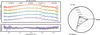 |
Fig. 7 Best-fit results from each atmospheric grid using the setup of run v07 for the companion CD-35 2722 b. On the left, we display the observed spectrum (black) and the best-fit models from each grid in the different colors, offset vertically for clarity. The |


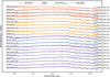 |
Fig. 8 Best spectral fit for each target. Here, the targets are organized by their derived Teff, from hottest at the top to coldest at the bottom. The Teff and S/N values are shown on the right side of each spectrum. The models are color-coded to indicate the grid that provided the best match to the data, selected based on the lowest |

4 Discussion
From our results, several important points emerge that can be grouped into two categories. First, the observed temperature-domain difference raises the question of whether the split has a physical explanation or whether it is a model-dependent feature related to the physics included in the different atmospheric models. Second, for the low-temperature targets, we measured the C/O ratio, a parameter often referred to as a formation tracer (Öberg et al. 2011). Here, we present these measurements along-side the possible implications for the formation histories of these targets.
4.1 Assessing the temperature-domain discontinuity
We begin by comparing the derived Teff values of our sample to their spectral types, shown in Figure 9. This figure includes several layers of information, which we will break down for clarity hereafter. First, the primary data points, represented by the large markers outlined in black, are the Teff results for the selected model among all five grids for each target. These points are color-coded depending on the best fit presented in Figure 8. This comparison shows that the hottest targets, which we modeled using ATMO and BT-Settl, closely follow the sixth-order polynomial fit from Filippazzo et al. (2015), which describes the relationship between Teff and spectral type for field brown dwarfs. However, for targets near spectral type M9, where Exo-REM and BT-SETTL+C/O yield the best solutions, we notice a particular shift in the trend toward lower Teff values. This behavior for young planetary-mass objects has been reported in previous studies, such as Filippazzo et al. (2015) and Bonnefoy et al. (2014), and is likely linked to the physical properties of the atmospheres of objects near the M/L transition. According to Filippazzo et al. (2015), young objects exhibit similar or slightly higher bolometric luminosities compared to field-age objects of the same spectral type. However, since they are still contracting, theirlarger radii require cooler photospheres to maintain the same luminosity. As a result, a lower log (ɡ) in young dwarfs could lead to reddening and a higher apparent spectral type. Further-more, the sensitivity of radius to age in young M8 – L0 dwarfs creates a significant dispersion in Teff, up to ~500 K, at the M/L transition. This dispersion could explain the deviations observed in our results for targets near M9, as these objects fall into the age and temperature regime where such variability is expected.
In addition to the large markers representing the best solutions (those with the lowest  ), Figure 9 includes smaller circles indicating the Teff values derived using each grid for each target, consistent with the respective Teff limits. From the smaller colored points in Figure 9, we observe that different grids behave distinctly. The Exo-REM grid, shown in purple, has an upper Teff limit of 2000 K and consistently yields solutions below the Filippazzo et al. (2015) fit for all our targets within its range. Next, BT-SETTL+C/O and BT-Settl, in blue and red, respectively, share similar underlying physics, but BT-SETTL+C/O explores an additional free parameter, accounting for changes in the atmospheric composition. Notably, at spectral type M9, BT-Settl shows a drop in the Teff solutions, aligning with the BT-SETTL+C/O and Exo-REM results, except for the L2 target, USco 1606-2219, which has a spectral type uncertainty of ±1. For BT-Settl, the same discontinuity was observed previously by Sanghi et al. (2023), and they attributed it to the fact that, since cloud opacity increases as Teff decreases, BT-Settl does not incorporate sufficient dust to accurately mimic the atmospheric behavior at these temperatures, leading to an underestimated Teff. For the Sonora Diamondback and ATMO model grids, we do not observe the same Teff drop. Their Teff solutions as a function of spectral type remain closely aligned with the trend observed for field dwarfs. This behavior is particularly interesting, as ATMO does not include clouds, and Sonora Diamondback assumes equilibrium chemistry only, meaning that this different behavior can potentially be explained by a lack of physics in these models to accurately represent the M/L transition.
To further investigate the similarities and differences among the grids, we present Figures 10 and 11, which illustrate how the spectral features in the K-band vary as different parameters are adjusted. Specifically, we selected two example spectra representing the two temperature domains of our sample: one at Teff =2700 K and one at Teff =1700 K, both at log (ɡ) =4 dex and solar [M/H] and C/O. In Figure 10, we display the case for the hotter spectrum at 2700 K, which lies within the parameter space explored by ATMO and BT-Settl. The figure contains four sub-panels, each demonstrating the impact of varying one of the grid parameters. Interestingly, we observe that the continuum shape of the BT-Settl spectrum changes significantly when Teff is altered by ± 150 K. In contrast, the same variation in ATMO produces a much less noticeable effect. For log (ɡ), neither grid shows substantial variations when adjusting the value by ±0.5 dex. However, we note that the K-band lines at 2.2 µm become deeper with increasing log (ɡ). To explore fingering convection, ATMO incorporates three additional parameters compared to BT-Settl: [M/H], C/O, and γ. Varying [M/H] and γ results in noticeable changes to the continuum shape, pointing towards a possible inverse proportionality among them. Here we did not explore the behavior of C/O due to the limited sampling of this parameter in the grid (only 3 points from 0.3 to 0.7), which, as evidenced by our fits always preferring values at 0.7 (see Tables B.1 to B.20), is incapable of reliable exploring this dimension.
For the colder targets in our sample, we have all five grids available, allowing us to make a comparison similar to the one in Figure 10 for models from all grids at Teff =1700 K, which we present in Figure 11. This time, the figure comprises six sub-panels as we explore additional dimensions, including C/ O and ƒsed, along with the previous ones. In the first panel, we show Teff variations of ±150 K. We observe that BT-Settl, Sonora Diamondback, BT-SETTL+C/O, and Exo-REM all show similar behavior: increasing Teff leads to a slight increase in the central bump while decreasing Teff results in a decrease, flattening the spectrum. More interestingly, ATMO exhibits a very different behavior overall. The continuum shape of the selected model differs significantly, and the Teff variations have almost no impact on the observed features. This raises questions about ATMO’s ability to represent the physics of these objects at these temperatures. For log (ɡ), we observe similar, strong effects across all grids, with ATMO again showing the least noticeable impact. Interestingly, log (ɡ) strongly affects the depth of the CO overtone. We can compare this to the fourth panel, which explores the variations due to changes in C/O for the Exo-REM and BT-SETTL+C/O grids, where we observe a similar impact. However, the negative C/O variations are more noticeable in BT-SETTL+C/O than in Exo-REM, potentially indicating a limitation in exploring sub-solar C/ O values with this grid, at least when the [M/ H] is set to solar. For the [M/H], only ATMO and Exo-REM explore non-solar values, showing different variations in the spectral features, making comparisons between these grids more challenging. For ATMO and Sonora Diamondback, we also demonstrate how γ and ƒsed affect the spectral features; however, we do not explore this further, as the effects are more pronounced over a wider wavelength range.
The K-band is a rich spectral region that exhibits a strong correlation between Teff and spectral type. As discussed, we observe a drop in Teff of around 500 K at the M-L transition. The available grids currently limit our ability to fully understand this transition, as they cannot be compared homogeneously across this critical point. One possible step to overcome these limitations would be to extend grids such as Exo-REM to higher Teff ranges, which would require the addition of missing opacity sources. Additionally, multi-band comparisons could provide a better understanding of the parameters that shape the spectra of these objects. However, both of these ideas are beyond the scope of the present work.
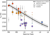 |
Fig. 9 Spectral type vs. Teff comparison. Large markers represent the best-model Teff values, presented in Figure 8. Smaller markers indicate the Teff solutions from all other grids, and gray points show the Teff predictions from evolutionary models. Companions in our sample are highlighted with square markers, and isolated targets are marked with circles. The black curve and gray area represent the relationship determined by Filippazzo et al. (2015) for field brown dwarfs. |
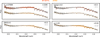 |
Fig. 10 Visualization of the two grids that reach the Teff domain of the hottest targets in our sample. Here, we compare models from both grids extracted at Teff = 2700 K, log (ɡ) = 4 dex, [M/H] = 0, and γ = 1.03, in black. In each panel, we illustrate the spectral variations caused by altering one parameter by the values listed in the upper right corner. The vivid color represents an increase, while the lighter (more transparent) color indicates a negative variation. |
 |
Fig. 11 Same as Figure 10, but comparing the five grids at parameters compatible with the coldest targets in our sample. Here the models presented in black are at Teff = 1700 K, log (ɡ) = 4 dex, [M/H] = 0, C/O = 0.55, γ = 1.03, and fsed = 4. |
4.2 Reliability of our posteriors
To understand and discuss the reliability of our posteriors, we categorized the different behaviors observed in our sample. As shown in Figure 8, our sample exhibits various S/N values and spans a broad range of Teff. This diversity allows us to assess the performance of the atmospheric grids under various conditions. To this end, we will make a broad distinction between the hot (M5 – M9) and the cold targets of our sample (M9 – L5).
Among the hot targets in our sample, several distinct behaviors emerge. KPNO Tau 1, KPNO Tau 6, USco 1606-2230, USco 1608-2335, and USco 1610-2239 demonstrate excellent alignment with predictions from evolutionary models and spectral type estimates, suggesting high confidence in the derived atmospheric parameters for these objects. In contrast, USco 1608-2232 and USco CTIO 108 A yield Teff solutions that are significantly hotter than expected from evolutionary models or spectral type relations but with very low  and a close match to the spectral features, especially for USco CTIO 108, indicating we can reliably report the physical properties (Teff and log (ɡ)) of these targets. CAHA Tau 1 and HR 7329 b converged towards solutions differing from evolutionary models’ log(ɡ) predictions, but providing overall a great spectral match. We urge special caution when referencing the parameters of USco 1610-2239 and USco 1608-2232, as the S/N for these observations is below 50, which, although still high, is among the lowest values in our sample. Finally, for the targets where ATMO provides the best match, as the continuum level is not well fitted for the longest wavelengths, the Teff could potentially be biased.
Among the cold targets in our sample, distinct behaviors can be identified. CD-35 2722 b and 2M 0103 AB b show strong agreement across all grids, indicating high confidence in the derived parameters for these objects. AB Pic b stands out as a low-Teff target with non-stellar metallicity values that align well with evolutionary model predictions, demonstrating the potential of grids to capture formation-tracing properties. However, several targets, including DH Tau b, FU Tau b, HIP 78530 b, KPNO Tau 4, USco 1606-2219, USco 1606-2335, and USco 1607-2239, exhibit poor agreement between atmospheric models and evolutionary model predictions for Teff. These discrepancies are likely influenced by the generally low S/N of their observations. Finally, USco 1612-2156 and USco 1613-2124 have data that is too noisy to yield reliable estimates of atmospheric parameters.
4.3 Formation tracers
To discuss the possible formation scenarios of our sample, we can explore the values of the so-called formation tracers, as well as the large-scale behavior of atmospheric properties. In broad terms, as expected, we observe no distinction in Teff and log (ɡ) behavior as a function of spectral type between isolated targets and companions. For example, in Figure 9, we have labeled the companions with square symbols and the isolated young brown dwarfs with circles. We observe that both groups follow the same trend, potentially suggesting a shared origin of formation for all these targets.
Regarding the formation tracers, with ForMoSA we only fit and constrain for the C/O ratio with Exo-REM, as it is the only grid that samples this dimension densely enough. In addition, because of the Teff range of Exo-REM and the S/N of our sample, we reliably measured C/O for a limited subset of our sample. As detailed in Sect. 4.2, these targets include the companions 2M0103 AB b, AB Pic b, and CD-35 2722 b. In Figure 12, we place our measured C/O ratios in the context of known values for other companions in the field. For the three targets in our sample, the C/O ratios are consistent with solar values. While this figure does not allow for definitive conclusions about formation histories, our targets fall well within the observed distribution, broadly consistent with the solar value revisited by Asplund et al. (2021). However, the C/O ratios for the reported targets in Figure 12 were measured differently across studies, complicating their comparison and interpretation. For now, we expect that as more observations are added to this plot, it will eventually enable us to draw population-based conclusions, including connections to other formation tracers, such as isotopologue ratios such as D/H and 12C/13C (Mollière & Snellen 2019; Zhang et al. 2022).
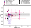 |
Fig. 12 Mass vs. C/O ratio for directly imaged companions, building on the work of Hoch et al. (2023). The magenta points represent the original sample of directly imaged planets, while the purple points indicate the three new measurements provided by this work. Recently published values have been added in black, including updated measurements for HR 8799 bcde (Nasedkin et al. 2024), AF Lep b (Balmer et al. 2025), β Pic b (Ravet et al., in prep.), YSES 1 bc (Zhang et al. 2024), and the Keck/KPIC sample published by Xuan et al. (2024). The dashed line and gray shaded area represent the solar C/O ratio with uncertainties (0.59 ± 0.1) as provided by Asplund et al. (2021). |
5 Conclusions
Our work underscores the importance of analyzing large datasets uniformly to gain a deeper understanding of planet formation and evolution, along with the atmospheric signatures of these processes. Using ForMoSA, we modeled a sample of 21 young substellar companions observed with VLT/SINFONI. This homogeneous analysis reveals several key conclusions.
First, we have observed that under a forward modeling approach, informing the priors is crucial. Allowing parameters such as the interstellar extinction and surface gravity to vary freely, without physical constraints, can lead to nonphysical or degenerate solutions. With the release of Gaia DR3, we now have access to high-precision distance measurements and 3D dust maps. This is one example of how invaluable the prior information can be, as it provides robust insights on some physical properties from unrelated measurements.
Next, we confirm that the K-band spectrum is a reliable proxy for estimating effective temperature. Our findings align with the Teff versus spectral type behavior identified by Bonnefoy et al. (2014) and Filippazzo et al. (2015) for young planetary-mass objects. The observed discontinuity in Teff occurs precisely at the M/L transition. However, current atmospheric models still fail to adequately capture the full range of relevant physical conditions across this transition, as previously identified by Sanghi et al. (2023) for BT-Settl. Therefore, there is a pressing need to further explore the discrepancies between self-consistent atmospheric model grids, which currently sample the parameter space unevenly and can produce diverging results.
Third, while we performed a homogeneous analysis of this unique library of SINFONI data, each target holds deeper mysteries. Many have also been observed with other instruments, which could provide valuable insights into their individual properties. Additionally, there are more SINFONI archival observations of companions, which were excluded from this study due to heavy stellar speckle contamination; however, they could potentially be revisited using advanced molecular mapping techniques, as was done for β Pic b in the work by Kiefer et al. (2024).
Finally, the lack of strong spectral differences in the K-band between wide-orbit planetary companions and isolated brown dwarfs suggests that they could have similar formation mechanisms. However, this remains an open question that requires further investigation through both observational and theoretical studies. We encourage the community to revisit and reanalyze archival datasets – not only those from SINFONI, but also those coming from legacy instruments. Such efforts may reveal insights that have long remained hidden.
Data availability
The flux-normalized SINFONI K-band spectra are available at the CDS via https://cdsarc.cds.unistra.fr/viz-bin/cat/J/A+A/701/A51. The files are available as .fits files with five columns, formatted as input for ForMoSA. The column names are WAV, FLX, ERR, RES, and INS, which correspond to the wavelength in μm, normalized flux in W m−2 μm−1, flux errors in the same units, spectral resolution, and instrument name, respectively. The flux scaling factors are available in Table A.3.
Acknowledgements
To the memory of Dr. France Allard and her contributions to the domain of atmospheric physics of stars, brown dwarfs, and exoplanets. We thank Carine Babusiaux for providing us with the Gaia measurements of interstellar extinction, derived using the 3D extinction map from Lallement et al. (2022). This publication utilized the SIMBAD and VizieR databases, operated by the CDS in Strasbourg, France. This work has utilized data from the European Space Agency (ESA) mission Gaia https://www.cosmos.esa.int/gaia, processed by the Gaia Data Processing and Analysis Consortium (DPAC, https://www.cosmos.esa.int/web/gaia/dpac/consortium). Funding for the DPAC has been provided by national institutions, particularly those participating in the Gaia Multilateral Agreement. We acknowledge support in France from the French National Research Agency (ANR) through project grants ANR-20-CE31-0012 (FRAME) and ANR-23-CE31-0006 (MIRAGES), as well as the Programmes Nationaux de Planetologie et de Physique Stellaire (PNP and PNPS). This project is supported in part by the European Research Council (ERC) under the European Union’s Horizon 2020 research and innovation program (COBREX; grant agreement no. 885593). P.P.B., M.B., and G.C. received funding from the French Programme National de Planétologie (PNP) and de Physique Stellaire (PNPS) of CNRS (INSU). S.P.’s research is supported by an appointment to the NASA Postdoctoral Program at the NASA–Goddard Space Flight Center, administered by Oak Ridge Associated Universities under contract with NASA.
Appendix A Background information for all targets
This appendix summarizes the properties and key information for each target. Table A.1 provides details of the observing runs. Tables A.2 and A.3 list the targets’ general properties and their references. Table A.1 provides an overview of each sample target’s observing conditions, including program IDs, principal investigators, and key observational setup parameters. The reported values of this table were extracted from the original FITS file headers. We observe that the observations were conducted under varying conditions, with some targets observed using the MACAO adaptive optics module while others were observed without it.
Observation log of the SINFONI Library.
General information about the SINFONI Library sample.
As mentioned above, in Tables A.2 and A.3, we provide an overview of the general properties of each object, organized in alphabetical order. The information is split into two main tables for clarity. Table A.2 lists the spatial coordinates, including right ascension and declination, the parallax in mas, and the corresponding distance in parsec. The last two columns provide details on the distance and age of each target. Table A.3 continues with the spectral type of each target, its apparent and absolute magnitudes in the K band, and the flux calibration factor for the SINFONI spectra in units of W m−2 μm−1. In the last column of this table, we also provide all the references used to gather the information about the targets.
In addition, Table A.4 provides various properties of the companion objects in our sample. Specifically, it includes information on the projected distance to their host stars, the spectral type of the host stars, and, when available, the metallicity of the host stars. For comparison, we also include the metallicity and C/O ratio measurements from our work for the targets where such data are available. The chemical composition of the Sun can be found in Asplund et al. (2021). The metallicity for the Taurus-Auriga association is provided by D’Orazi et al. (2011). More metallicities of young stellar associations can be extracted from Viana Almeida et al. (2009) and Torres et al. (2006). Additionally, a column is provided for specific comments or annotations regarding our measurements.
The last table included in this appendix summarizes all the properties derived from the evolutionary models. We have used the BHAC15 COND03 and DUSTY00 models from (Baraffe et al. 2015) to provide estimated values for the mass (MJup), Teff (K), log (ɡ) (dex), and radius (RJup). Specifically, we used the log (ɡ) values from the COND03 predictions as priors for our atmospheric models. The predictions presented here were based on the SPHERE IRDIS K12,2 filter. Since some of our targets have distances derived from their mean association distances, the evolutionary predictions for some targets should be interpreted with caution.
Second part of the general information for the SINFONI Library.
Evolutionary model predictions for the SINFONI Library.
Appendix B Result figures per target
In this appendix, we present an overview of each target’s previous findings as well as the best-fit models and posteriors derived for each grid with ForMoSA. For the posteriors, we include spider plots that provide a comparative view of the models’ predictions in terms of Teff, log (ɡ), and RV, with the shaded area representing 99.73% confidence intervals (3σ). The accompanying tables list the exact values for each posterior, with asymmetric uncertainty ranges representing a 1σ confidence interval.
2M 0103 AB b, also known as Delorme 1 AB b or SCR J0103–5515C, is a first-of-its-kind companion. Its discovery by Delorme et al. (2013) marked the first direct imaging detection of a planetary-mass companion orbiting a very low-mass stellar binary at a wide separation. Since then, it has been followed up with multiple instruments. Preliminary orbital constraints and stability analyses for the system have been presented by Blunt et al. (2017). In addition, ultra-violet, optical, and near-infrared observations have revealed several emission lines, such as Hα, Hβ, Brγ, among others (Ringqvist et al. 2023; Eriksson et al. 2020; Betti et al. 2022b,a). These studies have confirmed that the companion is still actively accreting material at an age of approximately 40 Myr, indicating unusually long-lived accretion in a low-mass substellar object. Interestingly, as shown in Figure B.1, we do not detect Brγ in these observations. However, we note an unusual feature in the data around ~2.15 μm, which could be due to systematics.
AB Pic b, is a substellar companion discovered by Chauvin et al. (2005) via direct imaging with VLT/NaCo. Follow-up spectro-scopic observations with VLT/SINFONI confirmed its nature as a young L0–L1 dwarf with intermediate surface gravity, estimating an effective temperature of approximately 2000 K and log (ɡ) around 4.0 (Bonnefoy et al. 2010). More recent studies have combined archival near-infrared spectroscopy and multi-band photometry to further constrain its atmospheric properties, suggesting a cooler temperature of ~1700 K, log(ɡ) ~4.5, and a solar-like C/O ratio of 0.58±0.08 (Palma-Bifani et al. 2023). In the same work an orbital analysis was performed using astrometry from NaCo and SPHERE, which suggests a semi-major axis of 190 au and a high inclination of ~90 degrees, though the eccentricity remains uncertain. In Palma-Bifani et al. (2023) and Gandhi et al. (2025), the authors discovered a spin–orbit misalignment, with an obliquity around ~90 degrees, suggesting that AB Pic b is tilted as Uranus in our solar system. In terms of the architecture of the system, Gaia-Hipparcos proper motion anomalies hint at a potential inner companion down to ~2 times the mass of Jupiter beyond 10 au (Palma-Bifani et al. 2023; Lagrange et al. 2025). While there is no evidence of ongoing accretion, in the SINFONI observations presented here, we do observe an emission peak at 2.16 μm, which might be Brγ, and is calling for further analysis. Finally, the wide separation and system architecture continue to raise questions about its formation, with a planet-like formation mechanism potentially more likely.
CAHA Tau 1 is a young, free-floating substellar object identified in the Taurus star-forming region. It was initially discovered by Quanz et al. (2010) during a deep imaging survey targeting planetary-mass candidates, and it was later spectroscopically confirmed as a member of the Taurus population by Luhman & Mamajek (2010). Its spectral features and luminosity are consistent with those of a very low-mass brown dwarf or a planetary-mass object, placing it near the deuterium-burning limit.
CD-35 2722 b was discovered by Wahhaj et al. (2011) as part of the Gemini NICI Planet-Finding Campaign via direct imaging at a projected separation of ~67 au, and it was confirmed as co-moving over two epochs. Near-IR spectroscopy determined it to be an L4 dwarf with moderately low gravity, with atmospheric model fits yielding a Teff of 1700–1900 K and mass estimates around 31 MJup based on bolometric luminosity and evolutionary models. Furthermore, CD-35 2722 b appears over-luminous in the near-IR bands compared to field dwarfs, consistent with its youth. Studies of substellar companion populations (e.g., Bowler et al. (2020), Bonavita et al. (2016)) place CD-35 2722 b as a rare, well-characterized young L-type companion, useful for constraining formation models and testing atmospheric evolution. The corresponding Figure 7 and Table 3 are located in the main text, as we also use this target to benchmark our methods.
DH Tau b is a companion located at a wide separation (~330 au) from the T Tauri star DH Tauri. Discovered via direct near-infrared imaging (Itoh et al. 2005), its companionship was confirmed through common proper motion and spectroscopy, which revealed CO and H2O signatures and an effective temperature in the 2500 K range (Itoh et al. 2005; Patience et al. 2012; Xuan et al. 2020), notably higher than the values found in this work. From high spectral resolution observations with KPIC at Keck, Xuan et al. (2024) measured a projected rotational velocity of υ sin(i) = 5.7 ± 1.0 km/s, which corresponds to approximately 10–15% of the breakup speed and is consistent with late-stage disk-regulated angular momentum transfer. Polarimetric observations with VLT/SPHERE-IRDIS revealed significant H-band linear polarization, attributed to a highly inclined circumplanetary disk misaligned with the circumstellar disk, providing the first direct detection of a circumplanetary disk around a directly imaged companion (van Holstein et al. 2021; Martinez & Kraus 2022). Additional surveys using SPHERE and Spitzer/IRAC probed for further companions or disks, setting constraints on disk mass and geometry (Wolff et al. 2017; Lazzoni et al. 2020; Martinez & Kraus 2022). However, even though there is a circumplanetary disk, we do not see any spectral features suggesting ongoing accretion. These findings collectively suggest that DH Tau b formed early in the system’s evolution, likely through disk fragmentation, retains a substantial circumplanetary disk, and exhibits slow rotation, perhaps due to magnetic coupling.
FU Tau B was initially discovered as a co-moving companion via near-infrared imaging (Luhman et al. 2009). Recent monitoring of its Hα emission over six consecutive nights (Wu et al. 2023) revealed mild variability but no burst-like accretion events, indicating ongoing, stable mass accretion. ALMA Band-7 (0.88 mm) continuum observations, however, did not detect any disk emission above ~120–210 μJy, suggesting either a low-mass circumplanetary disk or rapid radial dust drift (Wu et al. 2020). In the SINFONI K-band observations, where we do not observe evidence of ongoing accretion, however, the dataset is relatively noisy, and some residuals of sky emission lines might still be present. Altogether, FU Tau B might represent a rare example of an isolated, wide-separation, young substellar companion, useful for probing early accretion behavior and potentially the rapid dissipation of circumplanetary disks around low-mass companions.
HIP 78530 b was first identified in the Upper Scorpius association by Lafrenière et al. (2011). The early observations confirmed common proper motion and obtained near-IR (JHK) spectroscopy, revealing a low surface gravity and a Teff of ~2800 K, consistent with an M8 spectral type (Lafrenière et al. 2011). Positioned at a projected separation of ~710 au, HIP 78530 b ranks among the lowest mass ratio wide-orbit companions known (~0.009), with an estimated orbital period of ~12000 years (Lafrenière et al. 2011). Subsequent thermal infrared imaging (3–5 μm) and near-IR spectroscopy characterized its atmospheric properties further (e.g., Petrus et al. (2020)), yielding a consistent Teff and a mass between 21–25 MJup. In these studies, no IR excess from circumplanetary material was found.
HR 7329 b, also known as η Tel b and HD 181327 b, is a directly imaged substellar companion orbiting a young A-type star part of the β Pictoris moving group. It was first detected by Lowrance et al. (2000) and confirmed as a co-moving companion at a projected separation of ~192 au (Neuhäuser et al. 2011). HR 7329 A hosts a debris disk detected in mid-infrared, detected by Lebreton et al. (2012) and recently observed with JWST/MIRI by Chai et al. (2024), where the orbit of planet b and the architecture of the system were studied.
KPNO Tau 1, 4, and 6 are young brown brown dwarfs from the Taurus star-forming region and share a late-M spectral type; therefore, we group them. They were initially identified and spectroscopically classified by Briceno et al. (2002) and later characterized in more detail by Luhman et al. (2003). Their near-infrared spectral types confirm their substellar status, and follow-up studies, such as those by Bonnefoy et al. (2014) and Quanz et al. (2010), have supported their classification and atmospheric properties within the broader context of young brown dwarfs. Regarding the comparison of evolutionary models with the derived properties of forward modeling, we observe that KPNO Tau 4 might have a lower Teff than initially predicted. These objects typically show weak or absent Brγ emission, indicating low or episodic accretion activity, as expected for late-M objects at this evolutionary stage. Here we observe a potential accretion event through Brγ emission for KPNO Tau 6, as evident from the residuals in Figure B.10. Variability, a common feature among such young substellar sources, has also been reported by Vos et al. (2020) for brown dwarfs at the Taurus star-forming region, likely arising from heterogeneous cloud coverage or magnetic phenomena.
Here we also group the Upper Scorpius (USco) brown dwarfs from our sample, all of which are consistent with late-M to early-L type brown dwarfs. These targets are aged between 5 and 11 million years, and are located at approximately 145 parsecs (Lodieu et al. 2011; Petrus et al. 2020). From the mentioned surveys, their spectral classifications are broadly consistent. From the SINFONI data, it is worth highlighting that USco1606-2219 shows signs of Brγ emission (see the residuals in Figure B.11).
Same as Table 3 but for KPNO Tau 6
Same as Table 3 but for USco 1606-2219
Same as Table 3 but for USco 1606-2230
Same as Table 3 but for USco 1606-2335
Same as Table 3 but for USco 1607-2239
Same as Table 3 but for USco 1608-2232
Same as Table 3 but for USco 1608-2335
Same as Table 3 but for USco 1610-2239
Same as Table 3 but for USco 1612-2156
Same as Table 3 but for USco 1613-2124
Finally, USco CTIO 108 A is an interesting target, since this brown dwarf hosts a lower-mass wide orbit companion USco CTIO 108 b at a projected separation of about 670 au (Béjar et al. 2008). The system’s wide separation and low binding energy suggest it is weakly bound, and dynamic interactions with other stars in the region could lead to its eventual disruption, offering valuable insights into the formation and evolution of substellar companions.
Same as Table 3 but for USco CTIO 108 A
References
- Ackerman, A. S., & Marley, M. S. 2001, ApJ, 556, 872 [Google Scholar]
- Akeson, R. L., Jensen, E. L. N., Carpenter, J., et al. 2019, ApJ, 872, 158 [Google Scholar]
- Allard, F. 2014, in IAU Symposium, 299, Exploring the Formation and Evolution of Planetary Systems, eds. M. Booth, B. C. Matthews, & J. R. Graham, 271 [NASA ADS] [Google Scholar]
- Allard, F., Hauschildt, P. H., Alexander, D. R., Tamanai, A., & Schweitzer, A. 2001, ApJ, 556, 357 [Google Scholar]
- Allard, F., Homeier, D., Freytag, B., & Sharp, C. M. 2012, in EAS Publications Series, 57, eds. C. Reylé, C. Charbonnel, & M. Schultheis, 3 [NASA ADS] [CrossRef] [EDP Sciences] [Google Scholar]
- Amundsen, D. S., Baraffe, I., Tremblin, P., et al. 2014, A&A, 564, A59 [NASA ADS] [CrossRef] [EDP Sciences] [Google Scholar]
- Asplund, M., Grevesse, N., Sauval, A. J., & Scott, P. 2009, A&A Rev., 47, 481 [Google Scholar]
- Asplund, M., Amarsi, A. M., & Grevesse, N. 2021, A&A, 653, A141 [NASA ADS] [CrossRef] [EDP Sciences] [Google Scholar]
- Balmer, W. O., Franson, K., Chomez, A., et al. 2025, AJ, 169, 30 [NASA ADS] [Google Scholar]
- Baraffe, I., Homeier, D., Allard, F., & Chabrier, G. 2015, A&A, 577, A42 [NASA ADS] [CrossRef] [EDP Sciences] [Google Scholar]
- Baudino, J. L., Bézard, B., Boccaletti, A., et al. 2015, A&A, 582, A83 [NASA ADS] [CrossRef] [EDP Sciences] [Google Scholar]
- Baudino, J.-L., Mollière, P., Venot, O., et al. 2017, ApJ, 850, 150 [Google Scholar]
- Béjar, V. J. S., Zapatero Osorio, M. R., Pérez-Garrido, A., et al. 2008, ApJ, 673, L185 [CrossRef] [Google Scholar]
- Betti, S. K., Follette, K. B., Ward-Duong, K., et al. 2022a, ApJ, 941, L20 [NASA ADS] [CrossRef] [Google Scholar]
- Betti, S. K., Follette, K. B., Ward-Duong, K., et al. 2022b, ApJ, 935, L18 [NASA ADS] [CrossRef] [Google Scholar]
- Biller, B. 2017, Astron. Rev., 13, 1 [Google Scholar]
- Blain, D., Charnay, B., & Bézard, B. 2021, A&A, 646, A15 [EDP Sciences] [Google Scholar]
- Blunt, S., Nielsen, E. L., De Rosa, R. J., et al. 2017, AJ, 153, 229 [Google Scholar]
- Bonavita, M., Desidera, S., Thalmann, C., et al. 2016, A&A, 593, A38 [NASA ADS] [CrossRef] [EDP Sciences] [Google Scholar]
- Bonnefoy, M., Chauvin, G., Rojo, P., et al. 2010, A&A, 512, A52 [NASA ADS] [CrossRef] [EDP Sciences] [Google Scholar]
- Bonnefoy, M., Chauvin, G., Lagrange, A. M., et al. 2014, A&A, 562, A127 [NASA ADS] [CrossRef] [EDP Sciences] [Google Scholar]
- Booth, M., Del Burgo, C., & Hambaryan, V. V. 2021, MNRAS, 500, 5552 [Google Scholar]
- Boss, A. P. 1997, Science, 276, 1836 [Google Scholar]
- Bowler, B. P., Blunt, S. C., & Nielsen, E. L. 2020, AJ, 159, 63 [Google Scholar]
- Briceno, C., Luhman, K. L., Hartmann, L., Stauffer, J. R., & Kirkpatrick, J. D. 2002, ApJ, 580, 317 [Google Scholar]
- Burrows, A., Marley, M., Hubbard, W. B., et al. 1997, ApJ, 491, 856 [Google Scholar]
- Chabrier, G. 2005, in The Initial Mass Function 50 Years Later, eds. E. Corbelli, F. Palla, & H. Zinnecker (Dordrecht: Springer Netherlands), 41 [Google Scholar]
- Chabrier, G., Johansen, A., Janson, M., & Rafikov, R. 2014, in Protostars and Planets VI, eds. H. Beuther, R. S. Klessen, C. P. Dullemond, & T. Henning, 619 [Google Scholar]
- Chai, Y., Chen, C. H., Worthen, K., et al. 2024, ApJ, 976, 167 [Google Scholar]
- Charnay, B., Bézard, B., Baudino, J. L., et al. 2018, ApJ, 854, 172 [Google Scholar]
- Chauvin, G., Lagrange, A. M., Dumas, C., et al. 2004, A&A, 425, L29 [NASA ADS] [CrossRef] [EDP Sciences] [Google Scholar]
- Chauvin, G., Lagrange, A. M., Zuckerman, B., et al. 2005, A&A, 438, L29 [NASA ADS] [CrossRef] [EDP Sciences] [Google Scholar]
- Cheetham, A. C., Kraus, A. L., Ireland, M. J., et al. 2015, ApJ, 813, 762 [Google Scholar]
- Claret, A. 1998, A&A, 335, 647 [NASA ADS] [Google Scholar]
- Cridland, A. J., Pudritz, R. E., Birnstiel, T., Cleeves, L. I., & Bergin, E. A. 2017, MNRAS, 469, 3910 [NASA ADS] [CrossRef] [Google Scholar]
- Czesla, S., Schröter, S., Schneider, C. P., et al. 2019, Astrophysics Source Code Library [record ascl:1906.010] [Google Scholar]
- da Silva, L., Torres, C. A. O., de La Reza, R., et al. 2009, A&A, 508, 833 [NASA ADS] [CrossRef] [EDP Sciences] [Google Scholar]
- Delorme, P., Gagné, J., Girard, J. H., et al. 2013, A&A, 553, L5 [NASA ADS] [CrossRef] [EDP Sciences] [Google Scholar]
- Desgrange, C., Milli, J., Chauvin, G., et al. 2023, A&A, 680, A64 [NASA ADS] [CrossRef] [EDP Sciences] [Google Scholar]
- D’Orazi, V., Biazzo, K., & Randich, S. 2011, A&A, 526, A103 [NASA ADS] [CrossRef] [EDP Sciences] [Google Scholar]
- Eisenhauer, F., Abuter, R., Bickert, K., et al. 2003, SPIE Conf. Ser., 4841, 1548 [Google Scholar]
- Eriksson, S. C., Asensio Torres, R., Janson, M., et al. 2020, A&A, 638, L6 [NASA ADS] [CrossRef] [EDP Sciences] [Google Scholar]
- Faherty, J. K., Cruz, K. L., Rice, E. L., & Riedel, A. 2013, Mem. Soc. Astron. Italiana, 84, 955 [Google Scholar]
- Filippazzo, J. C., Rice, E. L., Faherty, J., et al. 2015, ApJ, 810, 158 [Google Scholar]
- Fitzpatrick, E. L., & Massa, D. 2007, ApJ, 663, 320 [Google Scholar]
- Gagné, J., Fontaine, G., Simon, A., & Faherty, J. K. 2018, ApJ, 861, L13 [Google Scholar]
- Gaia Collaboration (Brown, A. G. A., et al.) 2021, A&A, 649, A1 [NASA ADS] [CrossRef] [EDP Sciences] [Google Scholar]
- Gaia Collaboration (Vallenari, A., et al.) 2023, A&A, 674, A1 [NASA ADS] [CrossRef] [EDP Sciences] [Google Scholar]
- Gandhi, S., de Regt, S., Snellen, I., et al. 2023, ApJ, 957, L36 [NASA ADS] [CrossRef] [Google Scholar]
- Gandhi, S., de Regt, S., Snellen, I., et al. 2025, MNRAS, 537, 134 [Google Scholar]
- Hauschildt, P. H., Baron, E., & Allard, F. 1997, ApJ, 483, 390 [Google Scholar]
- Hayashi, C., & Nakano, T. 1963, Progr. Theor. Phys., 30, 460 [Google Scholar]
- Helling, C., Ackerman, A., Allard, F., et al. 2008, MNRAS, 391, 1854 [Google Scholar]
- Hoch, K. K. W., Konopacky, Q. M., Theissen, C. A., et al. 2023, AJ, 166, 85 [NASA ADS] [CrossRef] [Google Scholar]
- Ireland, M. J., Kraus, A., Martinache, F., Law, N., & Hillenbrand, L. A. 2011, ApJ, 726 [Google Scholar]
- Itoh, Y., Hayashi, M., Tamura, M., et al. 2005, ApJ, 620, 984 [NASA ADS] [CrossRef] [Google Scholar]
- Karalidi, T., Marley, M., Fortney, J. J., et al. 2021, ApJ, 923, 269 [NASA ADS] [CrossRef] [Google Scholar]
- Kiefer, F., Bonnefoy, M., Charnay, B., et al. 2024, A&A, 685, A120 [NASA ADS] [CrossRef] [EDP Sciences] [Google Scholar]
- Kraus, A. L., Shkolnik, E. L., Allers, K. N., & Liu, M. C. 2014, AJ, 147 [Google Scholar]
- Kumar, S. S. 2002, in IAU Symposium, 211, 3 [Google Scholar]
- Lachapelle, F.-R., Lafrenière, D., Gagné, J., et al. 2015, ApJ, 802, 61 [Google Scholar]
- Lafrenière, D., Jayawardhana, R., Janson, M., et al. 2011, ApJ, 730, 42 [Google Scholar]
- Lagrange, A.-M., Kiefer, F., Rubini, P., et al. 2025, A&A, accepted, [arXiv:2501.10488] [Google Scholar]
- Lallement, R., Vergely, J. L., Babusiaux, C., & Cox, N. L. J. 2022, A&A, 661, A147 [NASA ADS] [CrossRef] [EDP Sciences] [Google Scholar]
- Lazzoni, C., Zurlo, A., Desidera, S., et al. 2020, A&A, 641, A131 [NASA ADS] [CrossRef] [EDP Sciences] [Google Scholar]
- Lebreton, J., Augereau, J. C., Thi, W. F., et al. 2012, A&A, 539, A17 [NASA ADS] [CrossRef] [EDP Sciences] [Google Scholar]
- Leconte, J., Baraffe, I., Chabrier, G., Barman, T., & Levrard, B. 2009, A&A, 506, 385 [NASA ADS] [CrossRef] [EDP Sciences] [Google Scholar]
- Liu, M. C., Magnier, E. A., Deacon, N. R., et al. 2013, ApJ, 777, L20 [NASA ADS] [CrossRef] [Google Scholar]
- Lodders, K. 2010, in Astrophysics and Space Science Proceedings, 16, Principles and Perspectives in Cosmochemistry, eds. A. Goswami, & B. E. Reddy, 379 [Google Scholar]
- Lodieu, N., Dobbie, P. D., & Hambly, N. C. 2011, A&A, 527, A24 [NASA ADS] [CrossRef] [EDP Sciences] [Google Scholar]
- Lothringer, J. D., Rustamkulov, Z., Sing, D. K., et al. 2021, ApJ, 914, 12 [CrossRef] [Google Scholar]
- Lowrance, P. J., Schneider, G., Kirkpatrick, J. D., et al. 2000, ApJ, 541, 390 [Google Scholar]
- Luhman, K. L., & Mamajek, E. E. 2010, ApJ, 716, L120 [Google Scholar]
- Luhman, K. L., Briceño, C., Stauffer, J. R., et al. 2003, ApJ, 590, 348 [Google Scholar]
- Luhman, K. L., Mamajek, E. E., Allen, P. R., Muench, A. A., & Finkbeiner, D. P. 2009, ApJ, 691, 1265 [NASA ADS] [CrossRef] [Google Scholar]
- Madhusudhan, N. 2012, ApJ, 758, 36 [NASA ADS] [CrossRef] [Google Scholar]
- Manjavacas, E., Lodieu, N., Béjar, V. J. S., et al. 2019, MNRAS, 491, 5925 [Google Scholar]
- Marleau, G.-D., Coleman, G. A. L., Leleu, A., & Mordasini, C. 2019, A&A, 624, A20 [NASA ADS] [CrossRef] [EDP Sciences] [Google Scholar]
- Marley, M. S., & McKay, C. P. 1999, Icarus, 138, 268 [NASA ADS] [CrossRef] [Google Scholar]
- Marley, M. S., Saumon, D., Visscher, C., et al. 2021, ApJ, 920, 85 [NASA ADS] [CrossRef] [Google Scholar]
- Martin, E. C., Mace, G. N., McLean, I. S., et al. 2017, ApJ, 838, 73 [NASA ADS] [CrossRef] [Google Scholar]
- Martinez, R. A., & Kraus, A. L. 2022, AJ, 163, 36 [NASA ADS] [CrossRef] [Google Scholar]
- Miles, B. E., Biller, B. A., Patapis, P., et al. 2023, ApJ, 946, L6 [NASA ADS] [CrossRef] [Google Scholar]
- Mollière, P., & Mordasini, C. 2012, A&A, 547, A105 [NASA ADS] [CrossRef] [EDP Sciences] [Google Scholar]
- Mollière, P., & Snellen, I. A. G. 2019, A&A, 622, A139 [NASA ADS] [CrossRef] [EDP Sciences] [Google Scholar]
- Mollière, P., Molyarova, T., Bitsch, B., et al. 2022, ApJ, 934, 74 [CrossRef] [Google Scholar]
- Morley, C. V., Mukherjee, S., Marley, M. S., et al. 2024, ApJ, 975, 59 [NASA ADS] [CrossRef] [Google Scholar]
- Mukherjee, S., Fortney, J. J., Morley, C. V., et al. 2024, ApJ, 963, 73 [NASA ADS] [CrossRef] [Google Scholar]
- Nasedkin, E., Mollière, P., Lacour, S., et al. 2024, A&A, 687, A298 [NASA ADS] [CrossRef] [EDP Sciences] [Google Scholar]
- Neuhäuser, R., Ginski, C., Schmidt, T. O. B., & Mugrauer, M. 2011, MNRAS, 416, 1430 [Google Scholar]
- Nielsen, E. L., De Rosa, R. J., Macintosh, B., et al. 2019, AJ, 158, 13 [Google Scholar]
- Öberg, K. I., Murray-Clay, R., & Bergin, E. A. 2011, ApJ, 743, L16 [Google Scholar]
- Padoan, P., Kritsuk, A., Norman, M. L., & Åke Nordlund 2005, ApJ, 622, L61 [NASA ADS] [CrossRef] [Google Scholar]
- Palma-Bifani, P., Chauvin, G., Bonnefoy, M., et al. 2023, A&A, 670, A90 [NASA ADS] [CrossRef] [EDP Sciences] [Google Scholar]
- Palma-Bifani, P., Chauvin, G., Borja, D., et al. 2024, A&A, 683, A214 [NASA ADS] [CrossRef] [EDP Sciences] [Google Scholar]
- Patience, J., King, R. R., De Rosa, R. J., et al. 2012, A&A, 540, A85 [NASA ADS] [CrossRef] [EDP Sciences] [Google Scholar]
- Petrus, S., Bonnefoy, M., Chauvin, G., et al. 2020, A&A, 633, A124 [NASA ADS] [CrossRef] [EDP Sciences] [Google Scholar]
- Petrus, S., Bonnefoy, M., Chauvin, G., et al. 2021, A&A, 648, A59 [EDP Sciences] [Google Scholar]
- Petrus, S., Whiteford, N., Patapis, P., et al. 2024, ApJ, 966, L11 [NASA ADS] [CrossRef] [Google Scholar]
- Pollack, J. B., Hubickyj, O., Bodenheimer, P., et al. 1996, Icarus, 124, 62 [NASA ADS] [CrossRef] [Google Scholar]
- Quanz, S. P., Goldman, B., Henning, T., et al. 2010, ApJ, 708, 770 [Google Scholar]
- Rebolo, R., Zapatero Osorio, M. R., & Martín, E. L. 1995, Nature, 377, 129 [NASA ADS] [CrossRef] [Google Scholar]
- Rice, E. L., Barman, T., Mclean, I. S., Prato, L., & Kirkpatrick, J. D. 2009, ApJS, 186, 63 [Google Scholar]
- Ringqvist, S. C., Viswanath, G., Aoyama, Y., et al. 2023, A&A, 669, L12 [NASA ADS] [CrossRef] [EDP Sciences] [Google Scholar]
- Rossow, W. B. 1978, Icarus, 36, 1 [NASA ADS] [CrossRef] [Google Scholar]
- Sanghi, A., Liu, M. C., Best, W. M. J., et al. 2023, ApJ, 959, 63 [NASA ADS] [CrossRef] [Google Scholar]
- Sicilia-Aguilar, A., Henning, T., Linz, H., et al. 2013, A&A, 551, A34 [NASA ADS] [CrossRef] [EDP Sciences] [Google Scholar]
- Spiegel, D. S., Burrows, A., & Milsom, J. A. 2011, ApJ, 727, 57 [Google Scholar]
- Stone, J. M., Eisner, J., Skemer, A., et al. 2016, ApJ, 829, 39 [Google Scholar]
- Swastik, C., Banyal, R. K., Narang, M., et al. 2021, AJ, 161, 114 [Google Scholar]
- Torres, C. A. O., Quast, G. R., da Silva, L., et al. 2006, A&A, 460, 695 [NASA ADS] [CrossRef] [EDP Sciences] [Google Scholar]
- Torres, C. A. O., Quast, G. R., Melo, C. H. F., & Sterzik, M. F. 2008, in Handbook of Star Forming Regions, Volume II, 5, ed. B. Reipurth (ASPCS), 757 [NASA ADS] [Google Scholar]
- Tremblin, P., Amundsen, D. S., Mourier, P., et al. 2015, ApJ, 804, L17 [CrossRef] [Google Scholar]
- Tremblin, P., Chabrier, G., Baraffe, I., et al. 2017, ApJ, 850, 46 [CrossRef] [Google Scholar]
- Turrini, D., Schisano, E., Fonte, S., et al. 2021, ApJ, 909, 40 [Google Scholar]
- van der Marel, N., & Mulders, G. D. 2021, AJ, 162, 28 [NASA ADS] [CrossRef] [Google Scholar]
- van Holstein, R. G., Stolker, T., Jensen-Clem, R., et al. 2021, A&A, 647, A21 [EDP Sciences] [Google Scholar]
- Venot, O., Hébrard, E., Agúndez, M., et al. 2012, A&A, 546, A43 [NASA ADS] [CrossRef] [EDP Sciences] [Google Scholar]
- Viana Almeida, P., Santos, N. C., Melo, C., et al. 2009, A&A, 501, 965 [NASA ADS] [CrossRef] [EDP Sciences] [Google Scholar]
- Vos, J. M., Biller, B. A., Allers, K. N., et al. 2020, AJ, 160, 38 [NASA ADS] [CrossRef] [Google Scholar]
- Wahhaj, Z., Liu, M. C., Biller, B. A., et al. 2011, ApJ, 729 [Google Scholar]
- Wang, J. J., Ruffio, J.-B., Morris, E., et al. 2021, AJ, 162, 148 [NASA ADS] [CrossRef] [Google Scholar]
- Wenger, M., Ochsenbein, F., Egret, D., et al. 2000, A&AS, 143, 9 [NASA ADS] [CrossRef] [EDP Sciences] [Google Scholar]
- Wolff, S. G., Ménard, F., Caceres, C., et al. 2017, AJ, 154, 26 [Google Scholar]
- Wu, Y.-L., Bowler, B. P., Sheehan, P. D., et al. 2020, AJ, 159, 229 [NASA ADS] [CrossRef] [Google Scholar]
- Wu, Y.-L., Cheng, Y.-C., Huang, L.-C., et al. 2023, AJ, 166, 143 [Google Scholar]
- Xuan, J. W., Bryan, M. L., Knutson, H. A., et al. 2020, AJ, 159, 97 [NASA ADS] [CrossRef] [Google Scholar]
- Xuan, J. W., Hsu, C.-C., Finnerty, L., et al. 2024, ApJ, 970, 71 [CrossRef] [Google Scholar]
- Zhang, Y., Snellen, I., & Mollière, P. 2022, in BAAS, 54, 208.04 [Google Scholar]
- Zhang, Y., González Picos, D., de Regt, S., et al. 2024, AJ, 168, 246 [NASA ADS] [CrossRef] [Google Scholar]
- Zuckerman, B., & Song, I. 2004, ARA&A, 42, 685 [Google Scholar]
- Zuckerman, B., Song, I., & Bessell, M. S. 2004, ApJ, 613, L65 [Google Scholar]
mw-plot documentation: https://milkyway-plot.readthedocs.io
The SINFONI Pipeline: https://www.eso.org/sci/software/pipelines/sinfoni
EsoReflex Software: www.eso.org/sci/software/esoreflex
photutils documentation: https://photutils.readthedocs.io/en/stable/
ForMoSA stands for FORward Modeling tool for Spectral Analysis.
ForMoSA documentation: https://formosa.readthedocs.io
Pymultinest documentation: https://johannesbuchner.github.io/PyMultiNest/
extinction.fm07 documentation: https://extinction.readthedocs.io/en/latest/api/extinction.fm87.html
All Tables
All Figures
|
Fig. 1 Sky map showing the right ascension and declination curves, along with our 21 targets. The circle marks represent companions, while the star marks indicate isolated objects. The names of the different associations are indicated in black. |
| In the text | |
|
Fig. 2 Example of the first exposure of AB Pic b: the SINFONI raw observation (left), where each spectral slice (slitlet) is projected as vertical lines, compared to the reduced data cube delivered by EsoReflex for which we show the slice at λ = 1.95 (right), which shows a clear detection of the source at the center. |
| In the text | |
|
Fig. 3 Example of optimal aperture radius selection and spectra rejection criteria using the AB Pic b dataset. In each panel, each color represents a different exposure of AB Pic b. Left: values for the fitted continuum slope between 2.05 and 2.2 µm as a function of aperture radius. Two distinct domains are observed: for radii smaller than the optimal value, the slope increases steeply; for radii larger than the optimal value, the slope still varies but becomes more stable. Center: S/N estimated within the same wavelength range as in the left panel, plotted as a function of aperture radius. For each observation, we highlighted the maximum S/N value with a square. The aperture radius corresponding to this maximum is our final selected radius each time. Right: derivative of the slope (reported in the left panel) with respect to the aperture radius. Some targets exhibit a non-smooth, decreasing derivative; we reject those epochs. For AB Pic b, this resulted in the rejection of the entire dataset for the second night. |
| In the text | |
|
Fig. 4 Final extracted spectra for each of the 21 targets in the sample, organized and colored by their spectral type reported in the literature (see Table A.3). The errors are reported in gray, and the main absorption features are labeled at the top of the figure, also in gray. On the right, we annotate the flux scaling factor for each target in units of W m−2 µm−1, also reported in Table A.3. |
| In the text | |
|
Fig. 5 Exploration of the impact of Av on the derived posterior values of Teff and log (ɡ) for the ATMO grid of models. The Av value is indicated by the color of each symbol. In the top panel, we compare Teff and log (ɡ) from model runs v01 (Av = 0) and v04 (Av freely explored). Dashed lines connect the estimated values for a single target across the two runs. This shows that both Teff and log (ɡ) are highly degenerate with Av. In the lower panel, we perform a similar comparison between model runs v03 (Av = 0) and v07 ( |
| In the text | |
|
Fig. 6 Comparison of the posterior distributions using a uniform versus Gaussian prior on log (ɡ) for AB Pic b (v07 vs. v08 model predictions, shown in light blue and purple, respectively). The Gaussian prior mean value is marked with a blue cross on the log (ɡ) axis, based on the BHAC15 and COND03 evolutionary model predictions. We also marked the Teff predictions with a blue cross, although this was not used as prior information. For comparison, the solar values for [M/H] and the C/O ratio are shown as black stars. |
| In the text | |
|
Fig. 7 Best-fit results from each atmospheric grid using the setup of run v07 for the companion CD-35 2722 b. On the left, we display the observed spectrum (black) and the best-fit models from each grid in the different colors, offset vertically for clarity. The |
| In the text | |
|
Fig. 8 Best spectral fit for each target. Here, the targets are organized by their derived Teff, from hottest at the top to coldest at the bottom. The Teff and S/N values are shown on the right side of each spectrum. The models are color-coded to indicate the grid that provided the best match to the data, selected based on the lowest |
| In the text | |
|
Fig. 9 Spectral type vs. Teff comparison. Large markers represent the best-model Teff values, presented in Figure 8. Smaller markers indicate the Teff solutions from all other grids, and gray points show the Teff predictions from evolutionary models. Companions in our sample are highlighted with square markers, and isolated targets are marked with circles. The black curve and gray area represent the relationship determined by Filippazzo et al. (2015) for field brown dwarfs. |
| In the text | |
|
Fig. 10 Visualization of the two grids that reach the Teff domain of the hottest targets in our sample. Here, we compare models from both grids extracted at Teff = 2700 K, log (ɡ) = 4 dex, [M/H] = 0, and γ = 1.03, in black. In each panel, we illustrate the spectral variations caused by altering one parameter by the values listed in the upper right corner. The vivid color represents an increase, while the lighter (more transparent) color indicates a negative variation. |
| In the text | |
|
Fig. 11 Same as Figure 10, but comparing the five grids at parameters compatible with the coldest targets in our sample. Here the models presented in black are at Teff = 1700 K, log (ɡ) = 4 dex, [M/H] = 0, C/O = 0.55, γ = 1.03, and fsed = 4. |
| In the text | |
|
Fig. 12 Mass vs. C/O ratio for directly imaged companions, building on the work of Hoch et al. (2023). The magenta points represent the original sample of directly imaged planets, while the purple points indicate the three new measurements provided by this work. Recently published values have been added in black, including updated measurements for HR 8799 bcde (Nasedkin et al. 2024), AF Lep b (Balmer et al. 2025), β Pic b (Ravet et al., in prep.), YSES 1 bc (Zhang et al. 2024), and the Keck/KPIC sample published by Xuan et al. (2024). The dashed line and gray shaded area represent the solar C/O ratio with uncertainties (0.59 ± 0.1) as provided by Asplund et al. (2021). |
| In the text | |
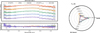 |
Fig. B.1 Same as Figure 7 but for 2M 0103 AB b |
| In the text | |
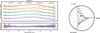 |
Fig. B.2 Same as Figure 7 but for AB Pic b |
| In the text | |
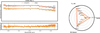 |
Fig. B.3 Same as Figure 7 but for CAHA Tau 1 |
| In the text | |
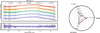 |
Fig. B.4 Same as Figure 7 but for DH Tau b |
| In the text | |
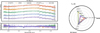 |
Fig. B.5 Same as Figure 7 but for FU Tau b |
| In the text | |
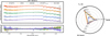 |
Fig. B.6 Same as Figure 7 but for HIP 78530 b |
| In the text | |
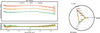 |
Fig. B.7 Same as Figure 7 but for HR 7329 b |
| In the text | |
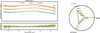 |
Fig. B.8 Same as Figure 7 but for KPNO Tau 1 |
| In the text | |
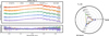 |
Fig. B.9 Same as Figure 7 but for KPNO Tau 4 |
| In the text | |
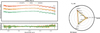 |
Fig. B.10 Same as Figure 7 but for KPNO Tau 6 |
| In the text | |
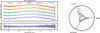 |
Fig. B.11 Same as Figure 7 but for USco 1606-2219 |
| In the text | |
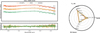 |
Fig. B.12 Same as Figure 7 but for USco 1606-2230 |
| In the text | |
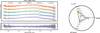 |
Fig. B.13 Same as Figure 7 but for USco 1606-2335 |
| In the text | |
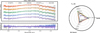 |
Fig. B.14 Same as Figure 7 but for USco 1607-2239 |
| In the text | |
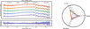 |
Fig. B.15 Same as Figure 7 but for USco 1608-2232 |
| In the text | |
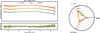 |
Fig. B.16 Same as Figure 7 but for USco 1608-2335 |
| In the text | |
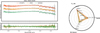 |
Fig. B.17 Same as Figure 7 but for USco 1610-2239 |
| In the text | |
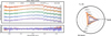 |
Fig. B.18 Same as Figure 7 but for USco 1612-2156 |
| In the text | |
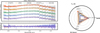 |
Fig. B.19 Same as Figure 7 but for USco 1613-2124 |
| In the text | |
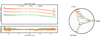 |
Fig. B.20 Same as Figure 7 but for USco CTIO 108 A |
| In the text | |
Current usage metrics show cumulative count of Article Views (full-text article views including HTML views, PDF and ePub downloads, according to the available data) and Abstracts Views on Vision4Press platform.
Data correspond to usage on the plateform after 2015. The current usage metrics is available 48-96 hours after online publication and is updated daily on week days.
Initial download of the metrics may take a while.